
Spatial Wave Measurement Based on U-net Convolutional Neural Network in Large Wave Flume

1
Department of Civil and Environmental Engineering, Faculty of Science and Engineering, Chuo University, Tokyo 192-0393, Japan
2
School of Computer Science and Engineering, Tianjin University of Technology, Tianjin 300384, China
3
Tianjin Research Institute of Water Transport Engineering Ministry of Transport, Tianjin 300456, China
4
CNOOC EnerTech-Drilling & Production Co., Tianjin 300450, China
*
Author to whom correspondence should be addressed.
Water 2023, 15(4), 647; https://doi.org/10.3390/w15040647
Submission received: 9 January 2023
/
Revised: 2 February 2023
/
Accepted: 3 February 2023
/
Published: 7 February 2023
(This article belongs to the Section Oceans and Coastal Zones)
Abstract
:This study proposed a spatial wave measurement method based on a U-net convolutional neural network. First, frame images are extracted from a video collected by a physical model experiment, and a dataset of spatial wave measurements is created and extended using a data enhancement method. A U-net convolutional neural network is built to extract the spatial wave information of the images; evidently, the segmented water level is close to that of the original image. Next, the U-net convolutional neural network is compared with the sensor, pixel recognition, and Canny edge detection methods. Pixel recognition results reveal that the maximum and minimum errors of the U-net convolutional neural network are 3.92% and 1.05%, those of the Canny edge detection are 5.97% and 1.33%, and those of the sensor are 11.8% and 1.6%, respectively. Finally, the nonlinear characteristic quantities of waves are measured using the proposed U-net convolutional neural network. The kurtosis and asymmetry calculated in the spatial domain are slightly larger than those calculated in the time domain, whereas the skewness calculated in the spatial domain is smaller than that calculated in the time domain. The asymmetry and kurtosis increase with an increase in wave height and period, whereas the skewness increases with an increase in wave height but decreases with an increase in period.
1. Introduction
When exploiting marine resources, numerous artificial structures must be built in the sea. These artificial buildings experience losses owing to wave impacts. To understand the impact and damage mechanism of waves on offshore buildings, marine and water conservancy researchers simulate real wave environments in a hydraulic laboratory to conduct relevant hydrodynamic research. In addition, while using marine resources to create opportunities for social development, the challenges posed by the ocean, such as natural marine disasters, including waves, sea ice, red tides, tsunamis, and storm surges, must be overcome [1,2]. Data on wave elements obtained by observing waves in experiments are necessary for scientific research. Because wave height and period are important wave elements, the measurement methods and their accuracy must be measured for marine engineering.
At present, methods for measuring wave heights in the laboratory can be split into two categories: measurements with wave height sensors and instruments that directly interact with the studied water body and noncontact measurements through processing images from videos of the studied water body. Traditional contact measurement methods include capacitance wave height sensors, buoy measuring instruments, accelerometers, and gyroscopes. To measure the wave height data, capacitive wave height sensors monitor changes in capacitance using the changes in the dielectric constant in different media. Capacitive wave-height sensors have the advantages of high measurement accuracy and fast response speed [3]. However, the sampling stability of the sensor decreases because tantalum wire is easily affected by impurities in water and charge is easily affected by electromagnetic fields. The buoy-measuring instrument primarily comprises measuring floats, data receivers, and mooring components. It monitors vertical voltage signals with changing wave height through a built-in gravity accelerometer to calculate wave elements, such as wave height and period [4]. However, the buoy measurement instruments are not suitable for laboratory environments because of their large size. The combination of accelerometer and gyroscope is used to collect carrier motion information, whereas the attitude matrix is used to convert the attitude angle information output by the gyroscope into the geographic coordinate system for processing; subsequently, the wave height is calculated [5]. However, the integral process is affected by temperature change, working conditions of the instrument, and other factors, which introduce artifacts to the observed results and affect accuracy [6]. The image-based method realizes noncontact measurements and avoids the measurement error caused by direct contact between the electronic sensing device and water body. However, the accuracy of its recognition and recognition of the wave measurement in complex environments, such as intense illumination, are affected [7]. For example, the BP neural network algorithm can measure wave height; however, it has poor numerical stability when predicting the water level height [8]. In addition, three traditional image segmentation methods are commonly employed: threshold-based, region-based, and edge detection-based segmentation [9]. The segmentation method based on the threshold value often does not consider spatial characteristics; thus, it is sensitive to noise and less robust. Further, the region growth method is slow and sensitive to noise, whereas the split merging method may destroy the region boundary. Edge detection cannot guarantee the continuity and sealing of edges, and the processing of higher-detail areas is insufficient, which can easily produce broken edges [10,11].
Nonlinearity is a crucial characteristic of waves and a key factor in the study of water wave dynamics. In the propagation process, wave nonlinearity increases wave height and wave steepness, and produces a wave with maximum height, which may cause serious marine accidents [12]. Therefore, the quantities of the nonlinear characteristics of waves must be studied. Numerous scholars have studied the nonlinearity of waves. Gao et al. [13,14] analyzed the time series and spatial distribution of the wave in a harbor subjected to regular waves, focused waves, and bichromatic short wave groups. Moreover, they discussed the effect of Bragg reflection on the harbor oscillation stimulated by regular incoming long waves. Yao et al. [15] verified a numerical simulation based on the Boussinesq equation through a physical model and applied the model to study the influence of reef morphological characteristics on wave motion. Wang et al. [16] studied the spatiotemporal distribution of the dynamic response of a sandy seabed under the action of regular and irregular waves through a series of large-scale model experiments. The effects of the wave height, wave period, and cover stone on the soil response near the water inlet were analyzed. Marino et al. [17] evaluated the formula for wave elevation recovery in pressure measurements and proposed a polynomial fitting method based on the unfiltered wave energy spectrum to analyze the sensitivity of each formula to a change in the cutoff frequency.
In this study, an image segmentation method based on deep learning was used to measure the wave height and period, and a U-net convolutional neural network was used for the image segmentation of a video of wave motion; unlike threshold segmentation, this method is not significantly affected by illumination. The main framework of this paper is as follows. Section 1 introduces the research significance and related work of this paper. Section 2 expounds the source of data, the basic principle of U-net convolutional neural network, the details of network training, and the evaluation index. In Section 3, we discuss the wave measurement results of U-net model and the comparison results with other methods (pixel identification, sensor and edge detection), and the wave measurement method using a U-net convolutional neural network was applied to study the nonlinear characteristic quantities of waves. Conclusions are drawn in Section 4.
2. Data and Method
2.1. U-net Basic Principles
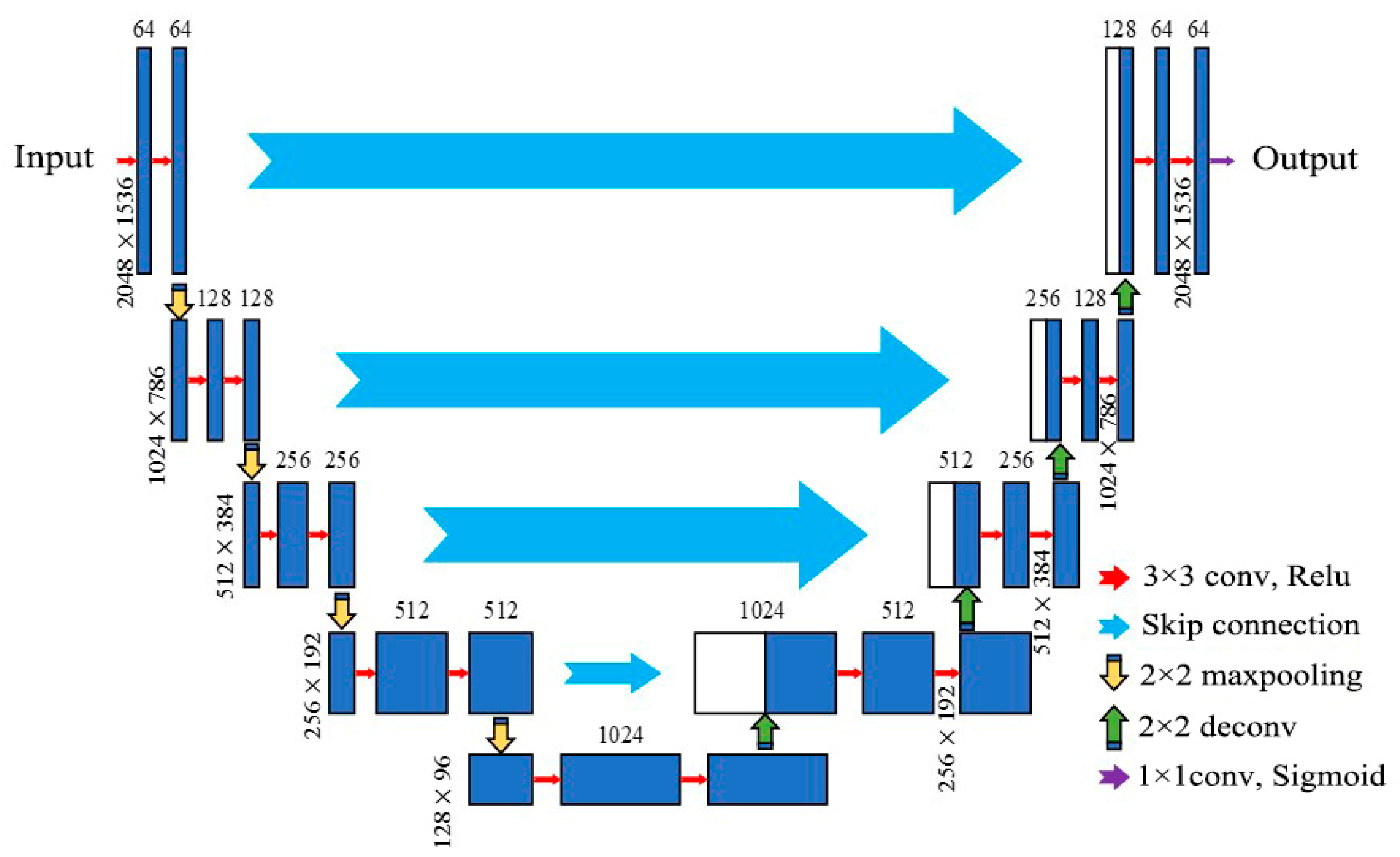
The proposed U-net convolutional neural network was built based on a full convolutional neural network, which essentially belongs to the coding-decoding model. The network architecture is shown in Figure 1. The entire network structure consists of two parts: shrinking (left part of Figure 1) and expanding paths (right part of Figure 1). The shrinking path is the encoding process, also called the downsampling process, whereas the extended path is the decoding process, also called the upsampling process. In the encoding process, each subsampling operation is used twice for image feature extraction in the same convolution, and the kernel size of the employed convolution is 3 × 3 × 3. After convolution, the ReLU activation function is used for activation, a 2 × 2 maximum pooling operation is performed to expand the global sensitivity field, and feature compression and subsampling operations are performed. During downsampling at each step, the number of feature channels is doubled, and the size of the feature graph is reduced to 1/2 of the previous one. After downsampling four times, upsampling begins at the decoding stage. The deconvolution operation for each upsampling reduces the number of feature channels to half of the previous one, and the size of the feature graph is twice that of the previous one. The size of the feature graph in the structure is shown as a number at the lower left corner of the convolutional block (blue rectangle), and the number of feature channels is shown as a number at the upper end of the convolutional block (blue rectangle). Finally, the number of feature channels is reduced to the required number using a 1 × 1 convolution kernel, and the sigmoid activation function is used for prediction classification. The key to the network lies in the feature fusion of the skip layer between the encoding and decoding processes, which reduces the loss of the underlying feature information caused by the maximum pooling operation in the encoding process to obtain high-quality segmentation results [18].
2.2. Data Sources and Data Preprocessing
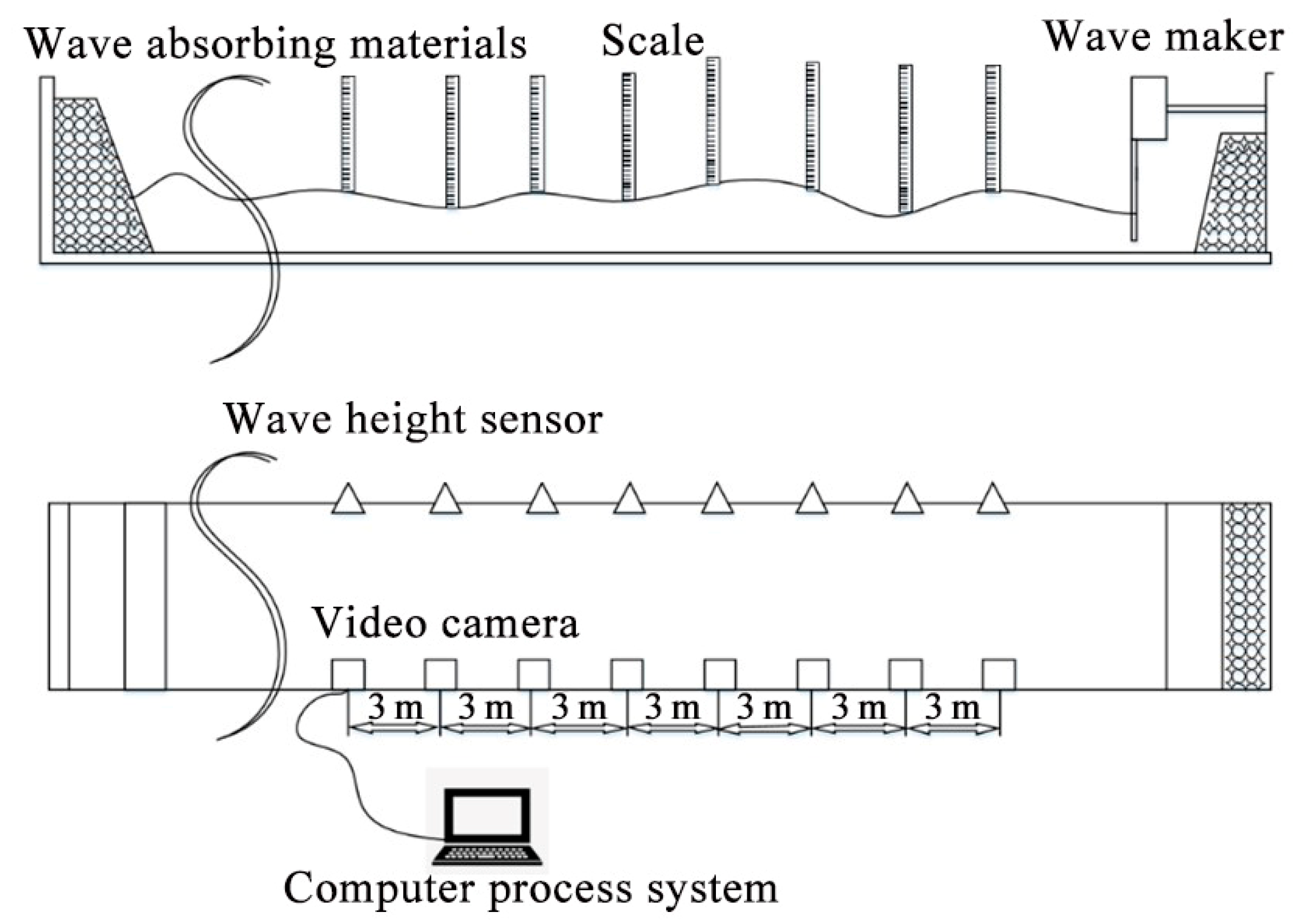
The data were collected from a model experiment of a large-scale wave flume. The length, width, and height of the large water tank were 450, 5, and 8–12 m, respectively. A wave-making machine was installed at one end of the water tank. It produced waves with a maximum height and period of 3.5 m and 2–10 s, respectively, which is similar to waves in the real ocean. The experimental setup is illustrated in Figure 2. Four built-in wave height sensors were used to measure the wave height, and high-definition cameras were installed on top of one side of a sink’s wall at 3 m intervals; a total of eight cameras were installed. The measuring range of the sensor used is 5 m, and the sampling interval is 0.05 s, that is, the sampling frequency is equal to 20 Hz. In order to be consistent with the acquisition frequency of the wave height sensor, the frequency of the camera is also set to 20 f/s, and the focal length of the camera lens is 6 mm. The camera lens angle completely covered the movement of the opposite wave, and its resolution was 2 cm. In this study, the 14 conditions listed in Table 1 were tested, the recorded video was stored in a computer, and continuous time 2048 × 1536 pixel high-definition photos were produced according to video frames. Distortion correction was performed using Zhang’s calibration method [19].
In this experiment, the static water level was 3.36 m, and seven groups were set in the regular and irregular wave experiments. In the regular wave group, the wave height of groups 1–4 remained unchanged and the period gradually increased, whereas the period of groups 1, 5, 6, and 7 remained unchanged and the wave height gradually increased. The height of irregular wave groups 8–11 remained unchanged and the period gradually increased, whereas the period of groups 8, 12, 13, and 14 remained unchanged and the wave height gradually increased. In addition, the experimental environments of groups 4, 7, 11, and 14 contained interference factors, such as wall damage or strong light exposure, and the specific operating parameters are listed in Table 1.
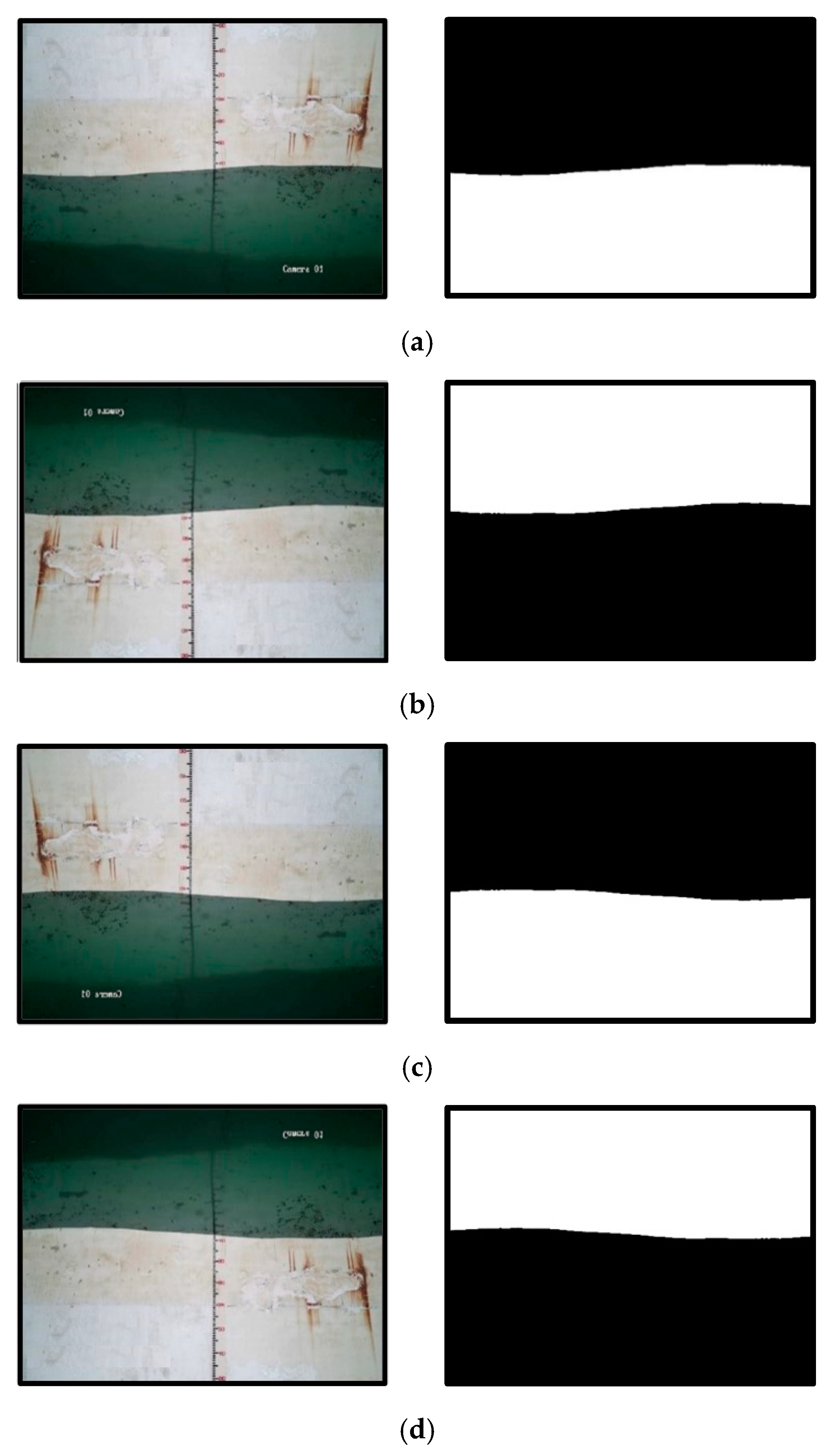
The U-net neural network is a supervised deep learning algorithm; therefore, the acquired images must be annotated before they are used on the network. In this study, the Labelme [20,21] tool was used to label the obtained images. The size of the dataset affects the performance of the deep learning model, and datasets with too few elements result in overfitting [22,23]. To this end, the data were enhanced through rotation, mirroring, and other methods based on the existing dataset [24]. In Figure 3, black represents the wall in the original picture, whereas white represents the water area.
2.3. Model Training
2.3.1. Training Conditions
In this study, Python and Pytorch deep learning frameworks were used to build a U-net neural network model, and the model training was completed on a laboratory graphics workstation. The specific configuration environment was Intel E5-2637 CPU, 64 GB, the GPU is Nvidia-M5000, 16 GB video memory, and Windows 10 operating system.
First, 1200 wave images were collected in the large scale wave flume experiment. After the data augmentation, the size of the dataset was tripled. Next, 80% of the data were randomly selected as the training set and the other 20% as the verification set. During model training, the sample size (batch size) used in one iteration was set to two.
2.3.2. Loss Function
Because this experiment is essentially a binary classification problem between the water body and background, the network model was required to only predict results in two situations: when the pixels in the image belonged to the wave and when the pixels in the image belonged to the background, namely, the wall of the sink. For each result, the prediction probabilities were p and 1 − p, respectively. Therefore, the loss function of the model used in this study was selected as the cross-entropy loss function that is commonly used in binary problems. It is calculated as shown in Equation (1).
where N Represents the total number of samples; yi represents the label of sample i, with yi = 0 and yi = 0 for the negative and positive classes, respectively; and pi is the probability that sample i is predicted to be positive.
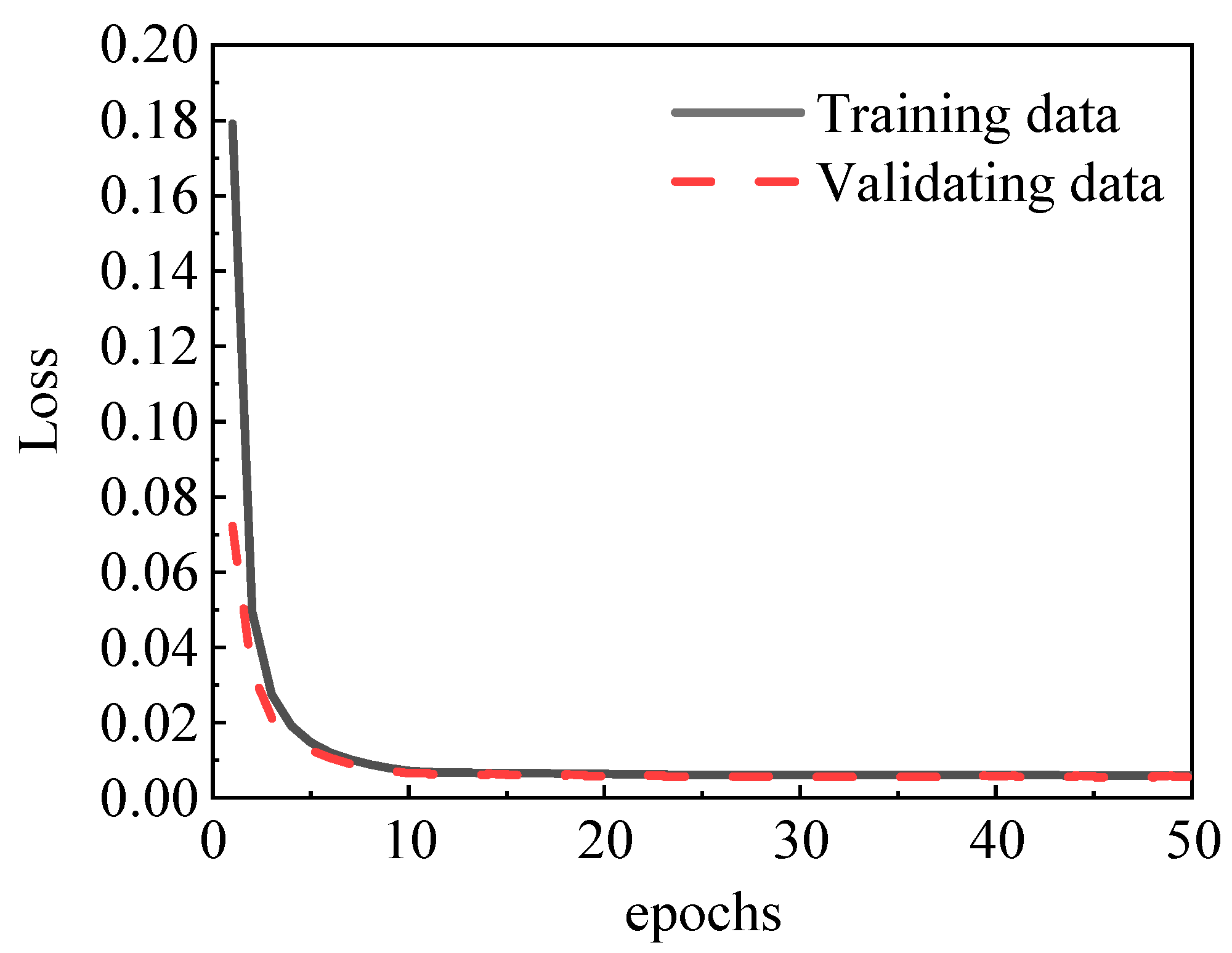
During the training process, the loss value decreased. Figure 4 shows the curve of the loss value of the model during training, which indicates that with an increase in training time, the error of the model gradually decreased and eventually converged.
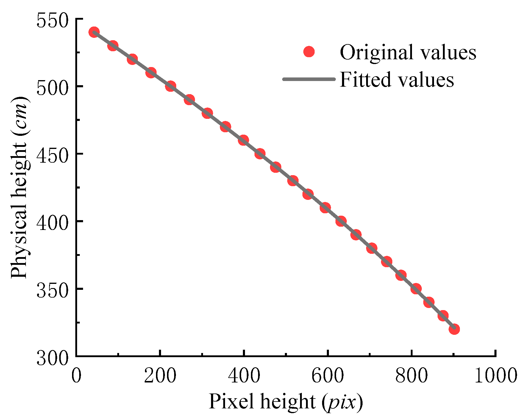
2.4. Scale Calibration
To convert the wave height in the image from pixel height to physical height, the pixel height must be fitted on the scale to the physical height it represents. The fitting method chosen in this experiment was quintic polynomial fitting. First, the camera position was fixed according to the experimental conditions. Next, an image was captured with an empty sink. Again, one pixel was taken every 10 cm along the scale from the top to the bottom. Finally, the ordinate value of each pixel and the actual height it represents were substituted into the following Equation (2).
where x represents the pixel height and y represents the physical height. Thus, the coefficients a, b, c, d, e, and constant f were determined, and finally, the calibration relationship of the scale was obtained to convert the spatial wave measurement value from pixel to physical height. Figure 5 shows the calibration relationship of the scale.
2.5. Evaluation Index
Two evaluation indices, intersection over union (IoU) and accuracy, were used to measure the performance of the model. The IoU indicator evaluates segmentation performance. The larger the IoU, the greater the overlap between the segmentation result and real label. IoU was calculated according to Equation (3). Accuracy is an evaluation index for evaluating the accuracy of the segmentation results; the higher the accuracy, the better the classifier. Accuracy was calculated according to Equation (4).
where P is the model prediction result and G is the actual label.
where TP is the number of positive cases correctly categorized by the neural network; TN is the number of negative cases correctly categorized by the neural network; P is the total number of positive cases; and N is the total number of negative cases.
Table 2 lists the changes in the IOU and accuracy of the model before and after data enhancement. Evidently, the accuracy of the model was further improved after dataset expansion through data augmentation.
3. Result
3.1. Spatial Wave Measurement Based on U-net Convolutional Neural Network
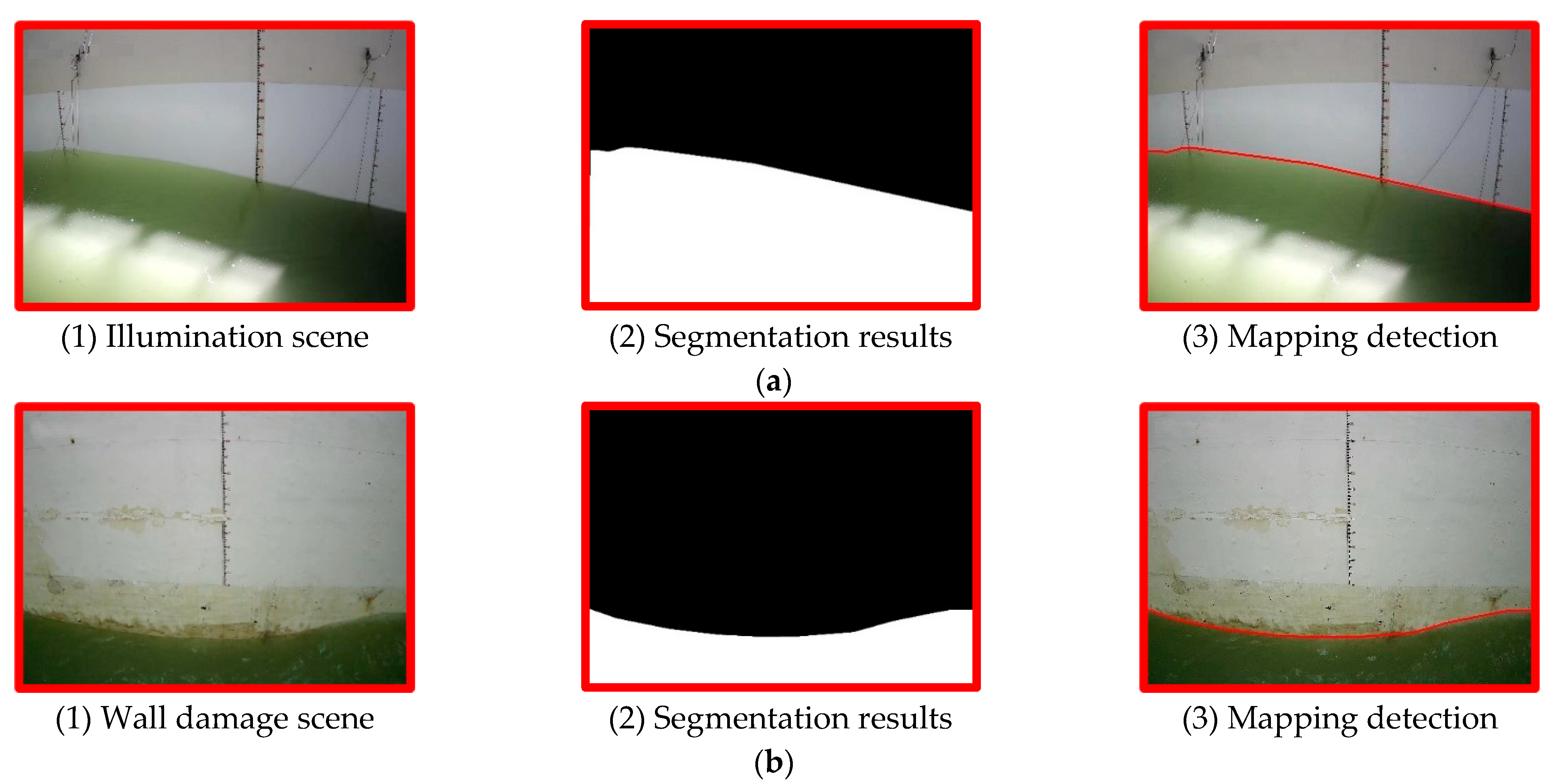
The segmentation performance of the U-net convolutional neural network on the spatial wave measurement after training is shown in Figure 6. After segmentation, the coordinates of the wave line in the image of the segmentation result were mapped to the original image. The water level of the segmentation result agreed with that in the original image. The results indicate that the U-net convolutional neural network can measure waves under the influence of strong interference factors and has a wider applicability.
3.2. Comparison of Space Wave Measurement Method Based on U-net and Other Methods
To demonstrate the effectiveness of the proposed U-net convolutional neural network, it was compared with the sensor, pixel recognition, and Canny edge detection methods, and the pixel recognition results were taken as reference values. Pixel recognition maximizes the display of the wave image, and manually reads the spatial wave measurement value of each frame image; additionally, the resolution of pixel recognition can reach 2 mm/pixel. Relying on the manual recognition of the spatial wave measurement value of each image is tedious and time-consuming, and has no practical application. However, its measurement results are reliable and can be used as reference measurement results to compare the accuracies of the image processing and wave height sensor measurement methods. The calculation method is shown in Equation (5).
where Cy is the actual distance represented by each pixel; Ymax is the actual height represented by the maximum value of the vertical pixel coordinates; Ymin is the actual distance represented by the minimum value of the vertical pixel coordinates; and Ny is the number of vertical pixels.
Canny edge detection was used to detect the wave line. First, threshold segmentation was performed on the wave and background in the image; subsequently, the horizontal G(x) and vertical gradient operators G(y) were used to calculate the horizontal and vertical gradient values of the wave image. Next, Equation (7) was used to calculate the size and direction of the image gradient to identify the wave line.
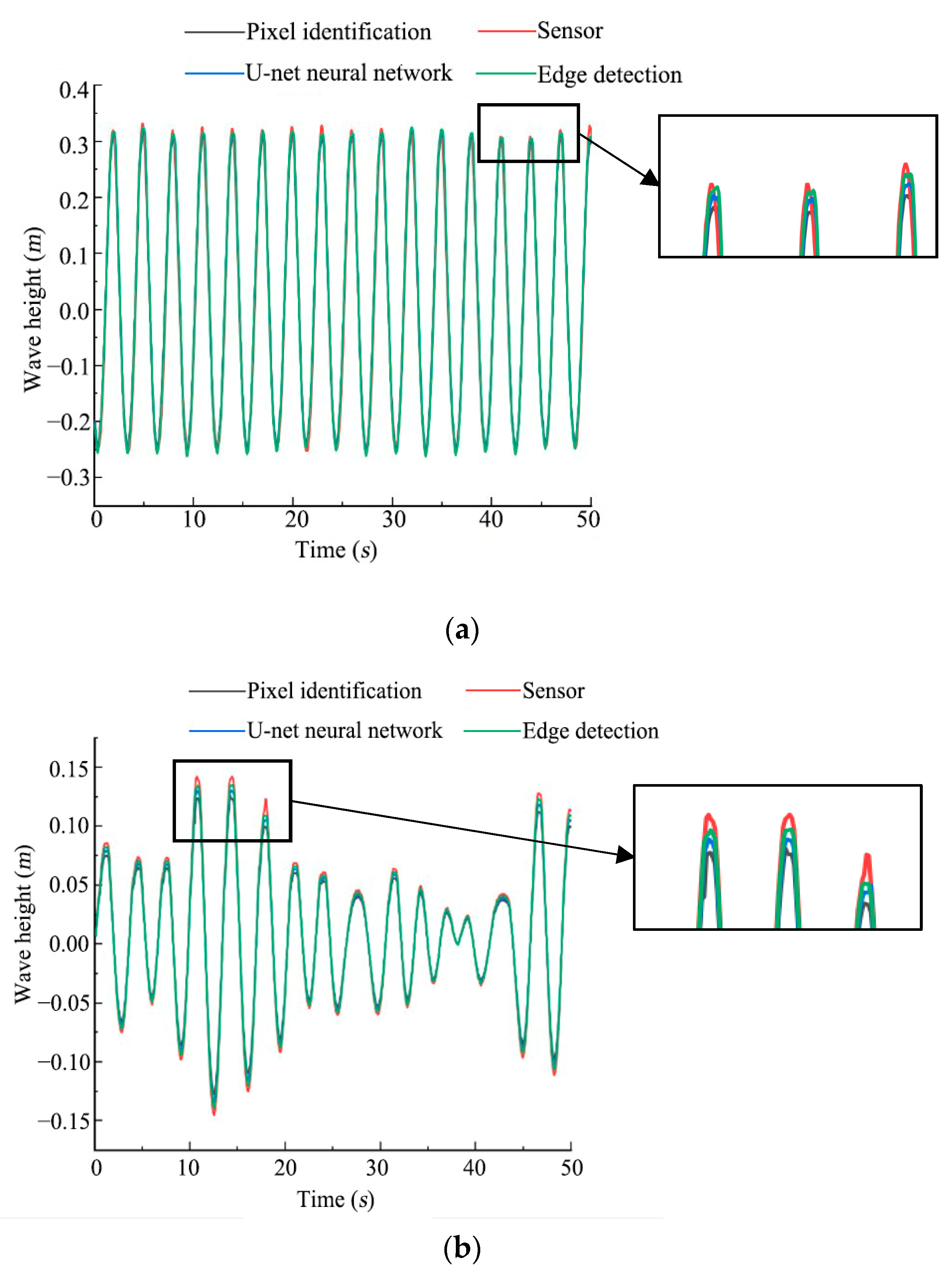
Figure 7 shows the change in the waveform measured using the four wave-measurement methods. The waveform curves of regular and irregular waves measured using the four measurement methods were in good agreement. However, at the wave crest, the wave height measured by the U-net convolutional neural network was closer to that measured by pixel recognition, whereas the value measured by the sensor was larger. This discrepancy was caused primarily by “hanging water” formed when the wave falls.
To quantitatively calculate the errors of data measured by different methods, this study used relative errors as the measurement index of the experimental results, and the calculation method is shown in Equation (8).
where δ is the relative error; h1 is the measured value; and h is the standard value based on pixel recognition.
Because edge detection cannot be used for wave measurement in strong interference environments, such as illumination and broken scene, the wave experiments of groups 4, 7, 11, and 14 in complex environments were measured, and errors were compared only for the wave height sensor and U-net convolutional neural network. All the experimental results are presented in Table 3.
Evidently from Table 3, in the regular wave experiment without interference in the ordinary environment, the maximum and minimum errors of the U-net convolutional neural network measurement were 2.54% and 1.05%, those of the edge detection measurement were 3.99% and 1.33%, and those of the sensor measurements were 6.17% and 1.6%, respectively. In the irregular wave experiment without interference, the maximum and minimum errors of the U-net convolutional neural network were 3.92% and 2.63%, those of edge detection were 5.97% and 3.63%, and those of sensor measurement were 11.8% and 6.84%, respectively. In summary, the measurement errors of the two image recognition measurement methods were smaller than those of the wave height sensor. Further, the U-net convolutional neural network had a higher measurement accuracy and wider application range compared with edge detection, which is more suitable for wave measurements in various complex laboratory environments.
In the regular wave experiment, when the wave was high, the error of the wave height sensor in measuring the wave height increased with an increase in wave period. When the wave period was constant, the error of the wave height sensor in measuring the wave height increased with increasing wave height. Similarly, in the irregular wave experiment, the measurement error of the wave height also increased with an increase in wave period and height, and the error was larger, thus demonstrating that the wave height sensor had some systematic error. In addition, the period measurement errors of the three wave measurement methods were relatively stable, all within 1%.
3.3. Study on Nonlinear Characteristic Quantity of Wave
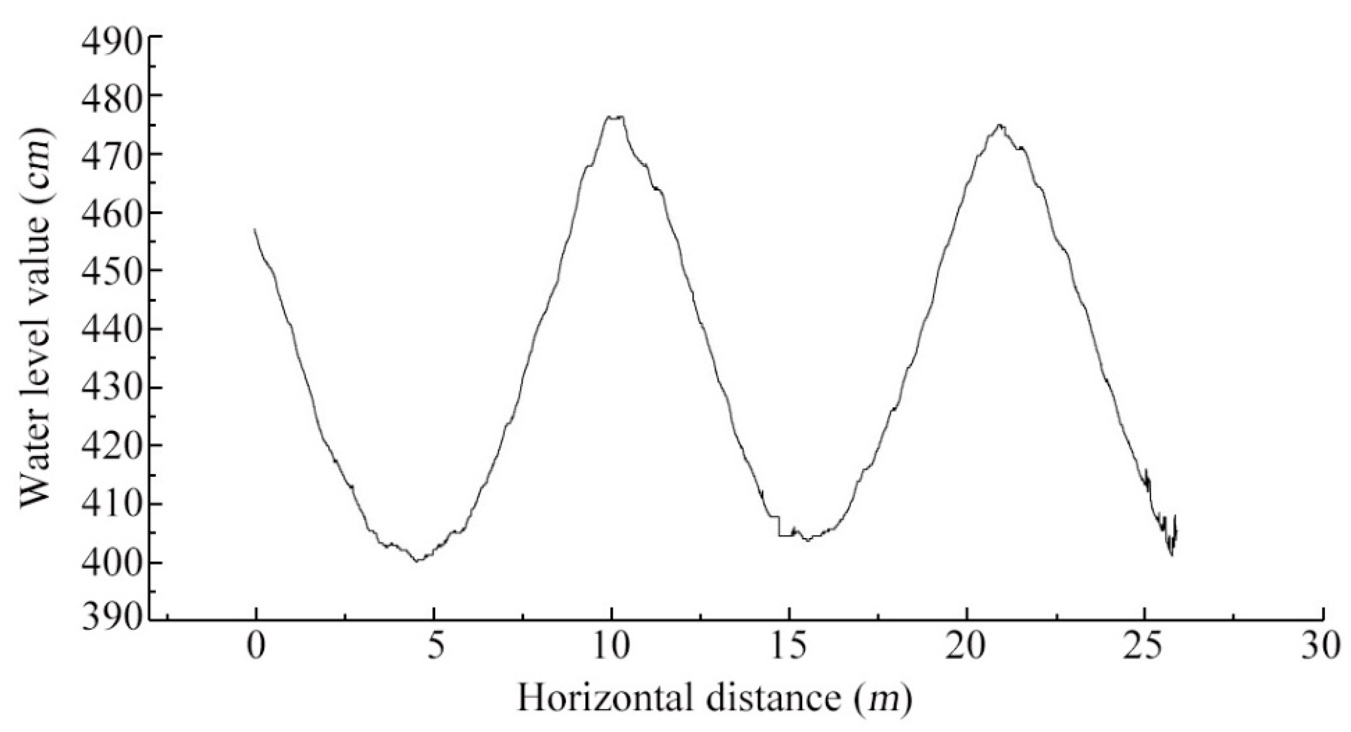
Based on the wave measurement of a single image, multi-stage continuous acquisition was performed in a wave tank at a large scale to fully investigate the spatial wave measurement at an ultra-long distance. In the test, seven cameras were continuously arranged in the test section of the wave water tank, and the width of each camera for transverse shooting was approximately 4 m. To ensure the complete splicing of the final waveform, adjacent cameras were oriented to have overlapping regions.
The principle of stitching is as follows. After the original image is converted into a processed binary graph, the coordinates of each pixel are extracted and converted into a scale value through the calibration relationship. Each scale is on the same horizontal line in the water tank. After a set of regular wave working condition data is obtained, the scale value of each adjacent image is recorded in the same coordinate system, the same ordinate is located, and the corresponding abscissa is determined. Only one positioning process is required. The point position is located in the program algorithm, and the scale value is extracted at each time step. Subsequently, a continuous spatial wave measurement can be established through fixed-point splicing. Figure 8 shows the filtered spatial wave.
In the process of wave propagation, owing to the influence of water depth and other factors, wave deformation occurs, thus resulting in the asymmetry of the wave shape. The nonlinear characteristic quantities of waves can be represented by the asymmetry, skewness, and kurtosis [25]. Asymmetry (A) refers to the degree to which a wave is asymmetrical about the vertical axis. When the degree of asymmetry (A) is positive, the wave leans forward and to the right relative to the vertical axis. When the asymmetry degree (A) is negative, the wave tilts backward and leans to the left relative to the vertical line. The degree of asymmetry can be calculated using Equation (9).
where A is the degree of asymmetry; H represents the Hilbert transform; η represents the wave surface elevation; represents the average wave surface elevation; and represents the average value.
Skewness (S) represents the degree of asymmetry of the wave surface with respect to the horizontal axis. When skewness is the third-order distance of a wave surface, it is defined by Equation (10).
where S is the skewness; η represents the wave surface elevation; represents the average wave surface elevation; and represents the average value. A positive skewness indicates that the wave crest becomes taller and sharper and the wave height becomes flatter and shallower.
Kurtosis (K) is used to indicate the degree of deviation between the distribution of the wave surface elevation and Gaussian distribution, and it is calculated according to Equation (11).
where K is the skewness; η represents the wave surface elevation; represents the average wave surface elevation; and represents the average value. The formula shows that kurtosis is the fourth-order distance of the wave surface. A Gaussian distribution corresponds to a kurtosis value of 3. When the kurtosis is greater than 3, the wave height distribution curve is sharper than that of the Gaussian distribution and its peak is higher. By contrast, if the kurtosis is less than 3, the wave height distribution is flatter than the Gaussian distribution.
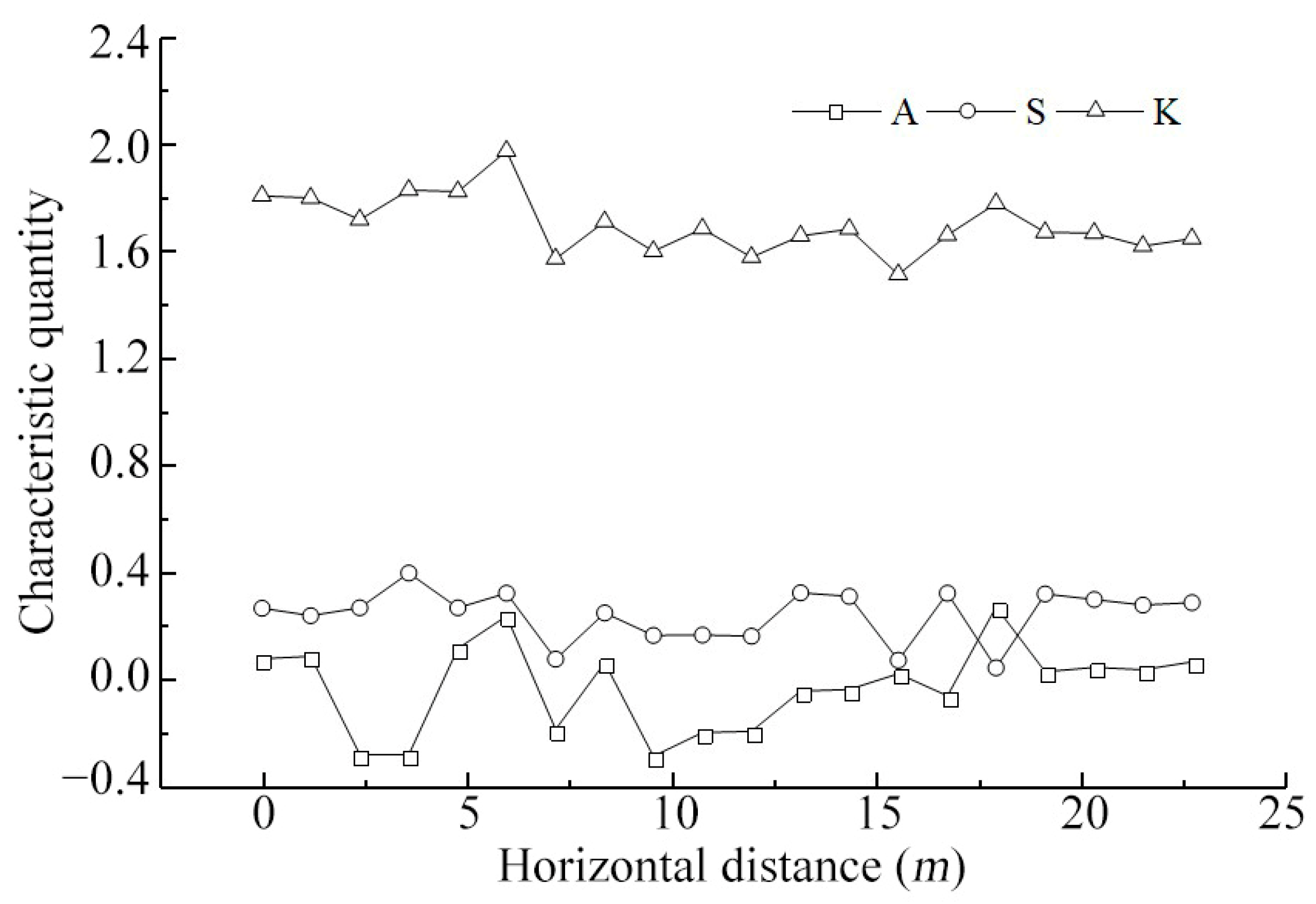
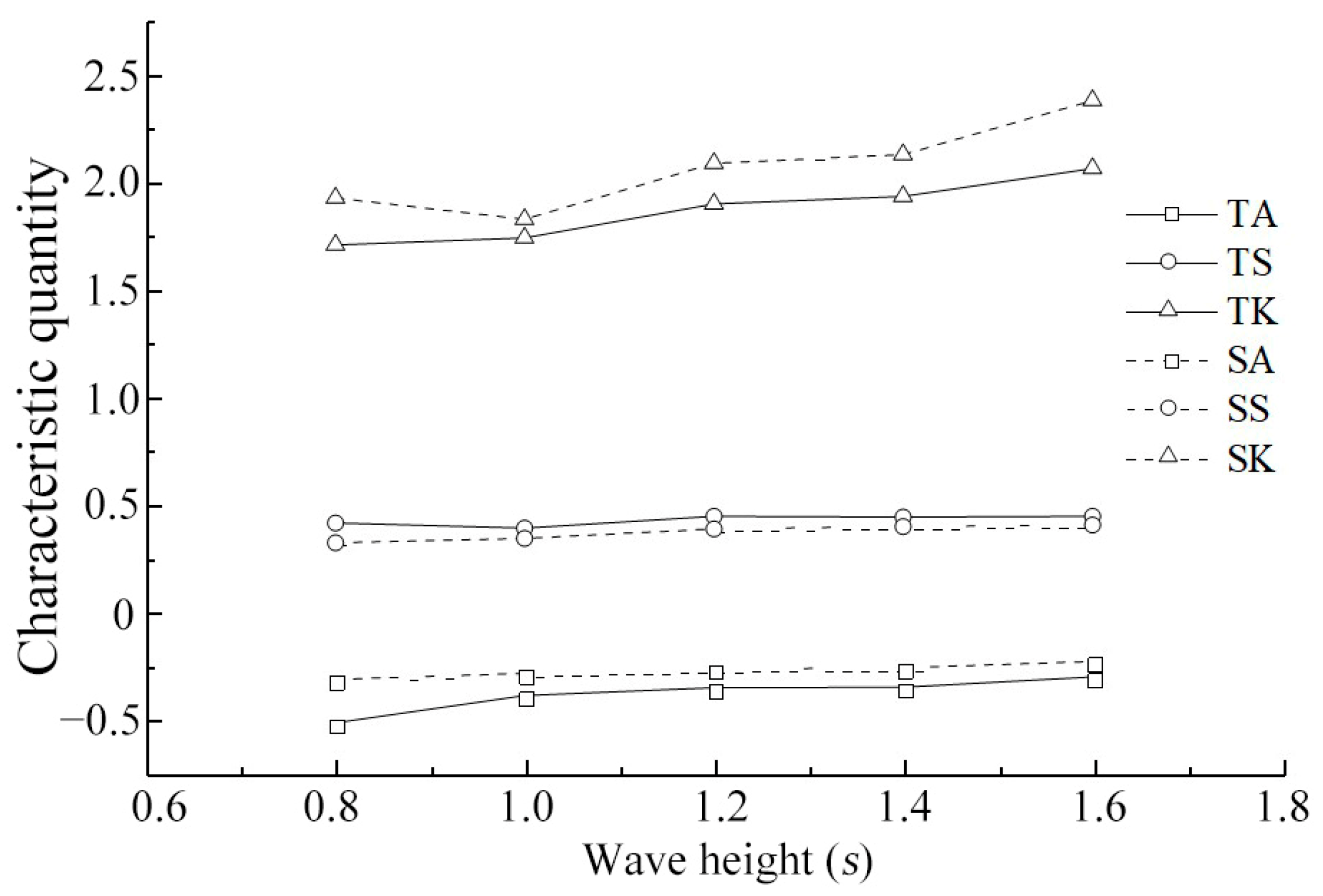
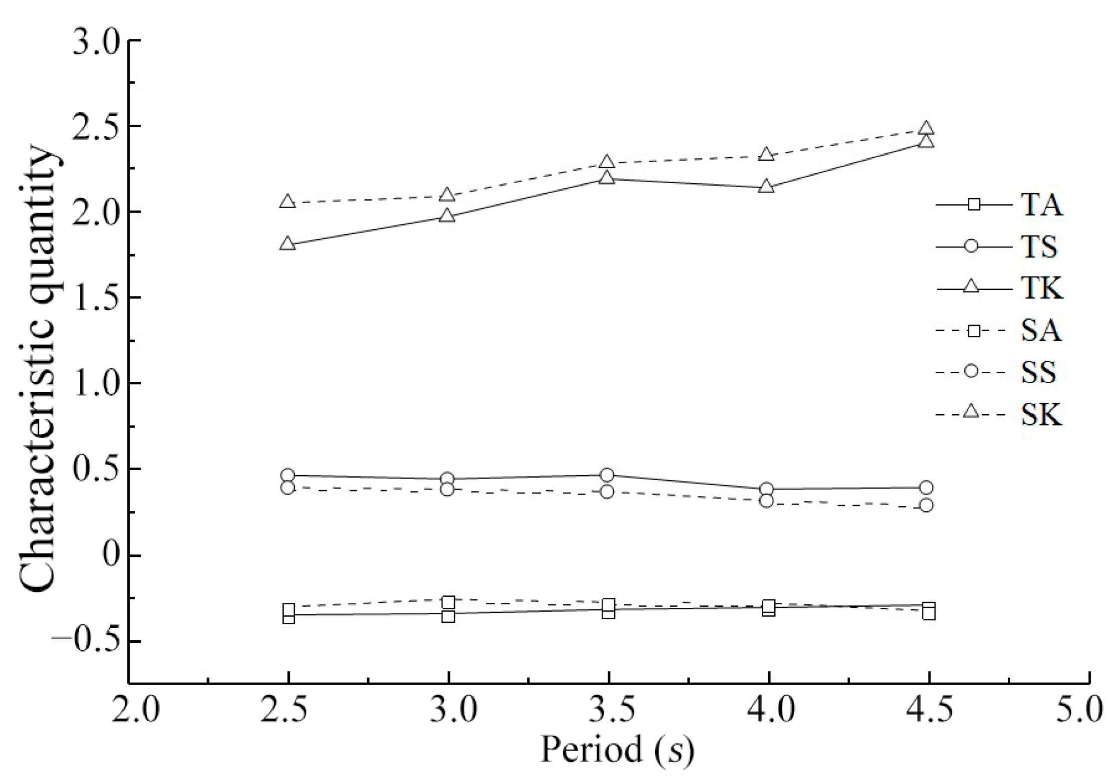
Using the above calculation method, the nonlinear characteristic quantity of a regular wave was calculated under the conditions of different point positions, wave heights, and periods. Figure 9 shows 20 points on a continuous 23 m spatial wave, and the nonlinear characteristic quantity of each point in its time domain was calculated. It exhibits some significant oscillations with regards to the spatial wave parameters. For the asymmetry the maximum and minimum are 0.26 and −0.3; for the skewness, the maximum and minimum are 0.41 and 0.03; and for the kurtosis, the maximum and minimum are 2.07 and 1.51. Thus, the traditional calculation method using the single point value will bring errors due to spatial oscillations. The issue can be solved when using results by U-nets in the spatial domain. Figure 10 shows the variation trends of asymmetry, skewness, and kurtosis with wave height in the time and space domains for different wave heights of regular waves. Only little difference between the two values in the space and time domains was observed. The kurtosis and asymmetry in the space domain were slightly larger than their nonlinear characteristic values in the time domain, whereas the skewness in the space domain was smaller than the calculated values in the time domain. Under the condition of the same period and different wave heights, the three characteristic quantities tended to increase with increasing wave height. Evidently from Figure 11, under different cycle conditions of regular waves, the distribution of the values was the same as that of different wave levels. For the same wave height and different period, the skewness decreased with an increase in period, whereas the asymmetry and kurtosis increased with an increase in period.
4. Conclusions
In this study, a spatial wave measurement method based on a U-net convolutional neural network was proposed. The method overcomes the influence of water movement on the measurement accuracy of electronic sensing devices and solves the measurement accuracy problem in complex environments, such as illumination. By converting a wave video shot by the camera into a series of pictures, a dataset for training the U-net convolutional neural network was constructed, and the network was optimized by reducing a loss function. The U-net method was found to be superior to the sensor and edge detection methods. In addition, the spatial nonlinear characteristic quantity of the wave was studied, the variation trends of asymmetry, skewness, and kurtosis in the time and frequency domains were obtained; thus, the spatial morphology of the wave was further understood.
Author Contributions
Conceptualization, J.C. and S.C.; methodology, J.C.; writing—original draft preparation, J.C.; supervision, S.C. and T.A.; data collection, Y.H. and Z.R.; writing—review and editing, S.C. and Y.H. All authors have read and agreed to the published version of the manuscript.
Funding
This research was funded by China National Key R&D Program(2022YFE0104500), the National Natural Science Foundation of China (no. 52001149, no. 52039005, no. 51861165102) and the Research Funds for the Central Universities (no. TKS20210102, no. TKS20220301, no. TKS20220601).
Data Availability Statement
Not applicable.
Conflicts of Interest
The authors declare no conflict of interest.
References
- Genç, R. Catastrophe of environment: The impact of natural disasters on tourism industry. J. Tour. Adventure 2019, 1, 86–94. [Google Scholar] [CrossRef]
- Chen, S.; Xing, J.; Yang, L.; Zhang, H.; Luan, Y.; Chen, H.; Liu, H. Numerical modelling of new flap-gate type breakwater in regular and solitary waves using one-fluid formulation. Ocean Eng. 2021, 240, 109967. [Google Scholar] [CrossRef]
- Ye, Y.; Zhang, C.; He, C.; Wang, X.; Huang, J.; Deng, J. A review on applications of capacitive displacement sensing for capacitive proximity sensor. IEEE Access 2020, 8, 45325–45342. [Google Scholar] [CrossRef]
- Jensen, R.E.; Swail, V.; Bouchard, R.H. Quantifying wave measurement differences in historical and present wave buoy systems. Ocean. Dyn. 2021, 71, 731–755. [Google Scholar] [CrossRef]
- Lee, S.C.; Huang, Y.C. Innovative estimation method with measurement likelihood for all-accelerometer type inertial navigation system. IEEE Trans. Aerosp. Electron. Syst. 2002, 38, 339–346. [Google Scholar]
- Wang, C.; Wang, S.; Chen, S.; Chen, S. Wave measurement method based on accelerometer and gyroscope. Sci. Technol. Eng. 2019, 19, 44–49. [Google Scholar]
- Ma, T.; Wang, S.; Chen, H.; Huang, M. Application of wave measurement based on optical method in wave shape study. J. Waterw. Harb. 2017, 38, 308–312. [Google Scholar]
- Chang, L.; Xie, J. Prediction of groundwater level by optimized neural network algorithm. Hydro-Sci. Eng. 2005, 4, 66–70. [Google Scholar]
- Huang, P.; Zheng, Q.; Liang, C. Overview of Image Segmentation Methods. J. Wuhan Univ. (Nat. Sci. Ed.) 2020, 6, 519–531. [Google Scholar]
- Hou, H.; Gao, T.; Li, T. Overview of image segmentation methods. Comput. Knowl. Technol. 2019, 15, 176–177. [Google Scholar]
- Xiao, F.; Qin, X. A Survey of Image Segmentation. PLC$FA 2009, 11, 77–79. [Google Scholar]
- Rapp, R.J.; Melville, W.K. Laboratory measurements of deep-water breaking waves. Philosophical Transactions of the Royal Society of London. Ser. A Math. Phys. Sci. 1990, 331, 735–800. [Google Scholar]
- Gao, J.; Ma, X.; Dong, G.; Chen, H.; Liu, Q.; Zang, J. Investigation on the effects of Bragg reflection on harbor oscillations. Coast. Eng. 2021, 170, 103977. [Google Scholar] [CrossRef]
- Gao, J.; Ma, X.; Zang, J.; Dong, G.; Ma, X.; Zhu, Y.; Zhou, L. Numerical investigation of harbor oscillations induced by focused transient wave groups. Coast. Eng. 2020, 158, 103670. [Google Scholar] [CrossRef]
- Yao, Y.; Zhang, Q.; Chen, S.; Tang, Z. Effects of reef morphology variations on wave processes over fringing reefs. Appl. Ocean. Res. 2019, 82, 52–62. [Google Scholar] [CrossRef]
- Wang, X.; Chen, S.; Wang, R.; Zhang, J.-M. Large wave flume tests on wave-induced response of sandy seabed adjacent a water intake. Ocean. Eng. 2020, 195, 106709. [Google Scholar] [CrossRef]
- Marino, M.; Rabionet, I.C.; Musumeci, R.E. Measuring free surface elevation of shoaling waves with pressure transducers. Cont. Shelf Res. 2022, 245, 104803. [Google Scholar] [CrossRef]
- Ronneberger, O.; Fischer, P.; Brox, T. U-Net: Convolutional Networks for Biomedical Image Segmentation. In Proceedings of the International Conference on Medical Image Computing and Computer-Assisted Intervention–MICCAI 2015, Munich, Germany, 5–9 October 2015. [Google Scholar]
- Wang, T.; Wang, L.; Zhang, W.; Duan, X.; Wang, W. Design of infrared target system with Zhang Zhengyou calibration method. Opt. Precis. Eng. 2019, 27, 1828–1835. [Google Scholar] [CrossRef]
- Russell, B.C.; Torralba, A.; Murphy, K.P.; Freeman, W.T. LabelMe: A Database and Web-Based Tool for Image Annotation. Int. J. Comput. Vis. 2014, 77, 157–173. [Google Scholar] [CrossRef]
- Torralba, A.; Russell, B.C.; Yuen, J. LabelMe: Online Image Annotation and Applications. Proc. IEEE 2010, 98, 1467–1484. [Google Scholar] [CrossRef]
- Tan, J.; Zhong, Y.; Huang, Z. Intelligent segmentation of rectal cancer based on U-net. Comput Era 2020, 8, 18–20+26. [Google Scholar]
- Mutasa, S.; Sun, S.; Ha, R. Understanding artificial intelligence based radiology studies: What is overfitting? Clin. Imaging 2020, 65, 96–99. [Google Scholar] [CrossRef] [PubMed]
- Buslaev, A.; Iglovikov, V.I.; Khvedchenya, E.; Parinov, A.; Druzhinin, M.; Kalinin, A.A. Albumentations: Fast and flexible image augmentations. Information 2020, 11, 125. [Google Scholar] [CrossRef]
- Soares, C.G.; Cherneva, Z.; Antão, E.M. Characteristics of abnormal waves in North Sea storm sea states. Appl. Ocean. Res. 2003, 25, 337–344. [Google Scholar] [CrossRef]
Figure 1.
Structure of the U-net neural network.

Figure 2.
Experiment layout.

Figure 3.
Data augmentation results. (a) Original image and its label, (b) Flip 180° clockwise and its label, (c) Horizontal mirroring and its labels, (d) Vertical mirroring and its labels.
Figure 3.
Data augmentation results. (a) Original image and its label, (b) Flip 180° clockwise and its label, (c) Horizontal mirroring and its labels, (d) Vertical mirroring and its labels.

Figure 4.
Loss curve of U-net model training.

Figure 5.
Scale calibration relationship.

Figure 6.
Segmentation results and mapping detection: (a) Segmentation results and mapping detection of illumination scene; (b) Segmentation results and mapping detection of the wall damage scene.
Figure 6.
Segmentation results and mapping detection: (a) Segmentation results and mapping detection of illumination scene; (b) Segmentation results and mapping detection of the wall damage scene.

Figure 7.
Comparison of waveform curves measured using four methods. (a) Group 6, (b) Group 9.

Figure 8.
Filtered spatial wave figure.

Figure 9.
Nonlinear feature quantity distributed along spatial points.

Figure 10.
Distribution of nonlinear characteristic quantities with wave height.

Figure 11.
Nonlinear characteristic quantity varies with period distribution. (The prefix T indicates the calculated value in the time domain, and the prefix S indicates the calculated value in the spatial domain).
Figure 11.
Nonlinear characteristic quantity varies with period distribution. (The prefix T indicates the calculated value in the time domain, and the prefix S indicates the calculated value in the spatial domain).


Table 1.
Experimental working condition parameter table.
| Groups | Water Level (m) | Environment | Wave Type | Wave Height (m) | Period (s) |
|---|---|---|---|---|---|
| 1 | 3.36 | Normal | Regular wave | 0.18 | 3 |
| 2 | 3.36 | Normal | Regular wave | 0.18 | 4.47 |
| 3 | 3.36 | Normal | Regular wave | 0.18 | 5.26 |
| 4 | 3.36 | Wall damage | Regular wave | 0.18 | 5.89 |
| 5 | 3.36 | Normal | Regular wave | 0.27 | 3 |
| 6 | 3.36 | Normal | Regular wave | 0.55 | 3 |
| 7 | 3.36 | Illumination | Regular wave | 0.83 | 3 |
| 8 | 3.36 | Normal | Irregular wave | 0.19 | 3.45 |
| 9 | 3.36 | Normal | Irregular wave | 0.19 | 4 |
| 10 | 3.36 | Normal | Irregular wave | 0.19 | 4.5 |
| 11 | 3.36 | Wall damage | Irregular wave | 0.19 | 5 |
| 12 | 3.36 | Normal | Irregular wave | 0.51 | 3.45 |
| 13 | 3.36 | Normal | Irregular wave | 0.62 | 3.45 |
| 14 | 3.36 | Illumination | Irregular wave | 0.78 | 3.45 |
Table 2.
Model indicators before and after data augmentation.
| Model Measure Index | IOU | Accuracy |
|---|---|---|
| Before data augmentation | 0.954 | 0.963 |
| After data augmentation | 0.985 | 0.984 |
Table 3.
Measurement error comparison.
| Groups | Measurement Method | Mean Period (s) | Mean Wave Height (m) | Period Error (%) | Wave Height Error (%) |
|---|---|---|---|---|---|
| 1 | Wave height sensor | 3.01 | 0.184 | 0.33 | 1.6 |
| Canny edge detection | 3 | 0.1835 | 0 | 1.33 | |
| U-net | 3 | 0.183 | 0 | 1.05 | |
| Pixel identification | 3 | 0.1811 | |||
| 2 | Wave height sensor | 4.5 | 0.187 | 0.67 | 3.14 |
| Canny edge detection | 4.48 | 0.1853 | 0.22 | 2.21 | |
| U-net | 4.48 | 0.184 | 0.22 | 1.49 | |
| Pixel identification | 4.47 | 0.1813 | |||
| 3 | Wave height sensor | 5.3 | 0.191 | 0.76 | 4.83 |
| Canny edge detection | 5.24 | 0.179 | 0.38 | 1.76 | |
| U-net | 5.24 | 0.18 | 0.38 | 1.21 | |
| Pixel identification | 5.26 | 0.1822 | |||
| 4 | Wave height sensor | 5.93 | 0.193 | 0.67 | 6.04 |
| U-net | 5.91 | 0.18 | 0.34 | 1.1 | |
| Pixel identification | 5.89 | 0.182 | |||
| 5 | Wave height sensor | 3 | 0.28 | 0 | 2.19 |
| Canny edge detection | 3 | 0.27 | 0 | 1.46 | |
| U-net | 3 | 0.277 | 0 | 1.1 | |
| Pixel identification | 3 | 0.274 | |||
| 6 | Wave height sensor | 3 | 0.585 | 0.33 | 6.17 |
| Canny edge detection | 3 | 0.573 | 0.33 | 3.99 | |
| U-net | 3 | 0.565 | 0.33 | 2.54 | |
| Pixel identification | 2.99 | 0.551 | |||
| 7 | Wave height sensor | 3 | 0.88 | 0 | 6.41 |
| U-net | 3 | 0.851 | 0 | 2.9 | |
| Pixel identification | 3 | 0.827 | |||
| 8 | Wave height sensor | 3.47 | 0.203 | 0.57 | 6.84 |
| Canny edge detection | 3.45 | 0.197 | 0 | 3.68 | |
| U-net | 3.45 | 0.195 | 0 | 2.63 | |
| Pixel identification | 3.45 | 0.19 | |||
| 9 | Wave height sensor | 4 | 0.21 | 0 | 8.8 |
| Canny edge detection | 4 | 0.2 | 0 | 3.63 | |
| U-net | 4 | 0.199 | 0 | 3.11 | |
| Pixel identification | 4 | 0.193 | |||
| 10 | Wave height sensor | 4.53 | 0.217 | 0.66 | 11.8 |
| Canny edge detection | 4.51 | 0.205 | 0.22 | 5.7 | |
| U-net | 4.51 | 0.2 | 0.22 | 3.1 | |
| Pixel identification | 4.5 | 0.194 | |||
| 11 | Wave height sensor | 5.03 | 0.218 | 0.6 | 13.5 |
| U-net | 4.98 | 0.199 | 0.4 | 3.65 | |
| Pixel identification | 5 | 0.192 | |||
| 12 | Wave height sensor | 3.46 | 0.549 | 0.29 | 7.64 |
| Canny edge detection | 3.44 | 0.533 | 0.29 | 4.5 | |
| U-net | 3.44 | 0.53 | 0.29 | 3.92 | |
| Pixel identification | 3.45 | 0.51 | |||
| 13 | Wave height sensor | 3.46 | 0.68 | 0.29 | 9.67 |
| Canny edge detection | 3.44 | 0.657 | 0.29 | 5.97 | |
| U-net | 3.44 | 0.643 | 0.29 | 3.71 | |
| Pixel identification | 3.45 | 0.62 | |||
| 14 | Wave height sensor | 3.47 | 0.88 | 0.57 | 12.53 |
| U-net | 3.44 | 0.812 | 0.29 | 3.84 | |
| Pixel identification | 3.45 | 0.782 |
Disclaimer/Publisher’s Note: The statements, opinions and data contained in all publications are solely those of the individual author(s) and contributor(s) and not of MDPI and/or the editor(s). MDPI and/or the editor(s) disclaim responsibility for any injury to people or property resulting from any ideas, methods, instructions or products referred to in the content. |
© 2023 by the authors. Licensee MDPI, Basel, Switzerland. This article is an open access article distributed under the terms and conditions of the Creative Commons Attribution (CC BY) license (https://creativecommons.org/licenses/by/4.0/).
Share and Cite
MDPI and ACS Style
Chen, J.; Hu, Y.; Chen, S.; Ren, Z.; Arikawa, T. Spatial Wave Measurement Based on U-net Convolutional Neural Network in Large Wave Flume. Water 2023, 15, 647. https://doi.org/10.3390/w15040647
AMA Style
Chen J, Hu Y, Chen S, Ren Z, Arikawa T. Spatial Wave Measurement Based on U-net Convolutional Neural Network in Large Wave Flume. Water. 2023; 15(4):647. https://doi.org/10.3390/w15040647
Chicago/Turabian StyleChen, Jiangnan, Yuanye Hu, Songgui Chen, Zhiwei Ren, and Taro Arikawa. 2023. "Spatial Wave Measurement Based on U-net Convolutional Neural Network in Large Wave Flume" Water 15, no. 4: 647. https://doi.org/10.3390/w15040647
Note that from the first issue of 2016, this journal uses article numbers instead of page numbers. See further details here.