
Dynamic Control of Yearly Drawdown Level of Overyear Regulation Reservoir in Cascade System
Hubei Key Laboratory of Digital River Basin Science and Technology, Huazhong University of Science and Technology, Wuhan 430074, China
*
Author to whom correspondence should be addressed.
Water 2023, 15(4), 665; https://doi.org/10.3390/w15040665
Submission received: 22 December 2022
/
Revised: 5 February 2023
/
Accepted: 6 February 2023
/
Published: 8 February 2023
(This article belongs to the Section Water Resources Management, Policy and Governance)
Abstract
:Based on the joint scheduling model of cascade reservoirs and a dynamic programming (DP) algorithm, this paper studies the optimal control of the yearly drawdown level of an overyear regulation reservoir considering the influence of inflow uncertainty. An innovative dynamic control method has been put forward, and the corresponding technical route is provided. In case study, the seven reservoirs of the Yalong River are used as the research object, the proposed dynamic control method is verified by a detailed case study, and yearly drawdown level dynamic control bounds of the Lianghekou reservoir under two inflow series are constructed. Based on a long series of historical inflows, the simulation calculation and detailed comparative analysis are carried out. It is found that the dynamic control bound constructed by the selected inflow series has little impact on the fluctuation of scheduling results and can well cope with the impact of inflow uncertainty on the scheduling results. In addition, compared with the traditional fixed-yearly-drawdown-level control mode, the proposed dynamic control method can consider the interannual difference of inflow, which can increase the total power generation of the cascade system by more than 94 billion kWh at maximum and realize 63.4%~76.3% of the benefits of the lifting space of yearly drawdown level optimization.
1. Introduction
We all know that hydropower energy is a very good green energy source; it can be obtained through the construction of reservoir–hydropower station systems [1,2,3]. According to the storage capacity, reservoirs can be divided into daily regulation reservoirs, seasonal regulation reservoirs, yearly regulation reservoirs, overyear regulation reservoirs, etc. [4].
With the rapid recent development of river basin and engineering technology [5], the cascade reservoir system has been gradually formed, and more and more overyear regulation reservoirs have appeared [6]. Due to the large storage capacity and greater energy storage of the overyear regulation reservoir, its scheduling mode will not only affect the interannual water distribution in the basin, but also directly affect the power generation efficiency of the entire cascade system. Therefore, for an overyear regulation reservoir in a cascade reservoir system, how to determine the best scheduling mode for many years has a great impact on the overyear regulation reservoir itself and the overall power generation of the cascade system.
To date, the research on the scheduling mode of overyear regulation reservoirs has mainly focused on the determination of an optimal yearly drawdown level [7]. For example, Yuan and Wang established an optimal model to simulate the year-end water level of a multi-year regulating reservoir based on a co-evolution differential evolution algorithm, and the model was validated using the case of the Wujiang cascade reservoirs [8]. Zhang et al. used a data-mining technique to identify the operational rules of the year-end level for a cascade reservoir system and presented an operational model of a decision tree based on the iterative dichotomizer 3 algorithm [9]. Wang et al. developed an operational model to calculate the optimal year-end water level of the Longyangxia reservoir and analyzed the impacts of the runoff and year-start water level on the year-end water level [10]. Liu et al. studied the year-end water level problem by using two prediction methods, which were a multi-objective decision model and a statistical regression predictive function, and compared their advantages and application conditions [11].
However, existing research has mostly focused on the scheduling of a single overyear regulation reservoir, in which the connection between the upstream and downstream water quantity and head is not considered [12,13,14]. The average annual inflow volume variations have an important influence on the long-term operation of the cascade system, and the change of the operational rules of the year-end level will have an important influence on the average annual hydropower yield [15]. Therefore, it is necessary to study the optimal scheduling mode of an overyear regulation reservoir in a cascade reservoir system. Here, the most important thing is to obtain the optimal dynamic yearly drawdown level rather than a fixed value which does not take into account the frequency difference in the inflow between years [16]. In fact, the inflow uncertainty will make the optimal yearly drawdown level a controlled range rather than a single value.
In view of this, this paper takes the overyear regulation reservoir in a cascade system as the research target and studies the construction and optimization problem of the dynamic control bound of the yearly drawdown level. To consider the influence of interannual differences in the inflow on the yearly drawdown level, the optimal dynamic control method of the yearly drawdown level of the Lianghekou reservoir under different inflow frequency series is designed based on the optimal scheduling results of multidimensional dynamic programming (DP). On this basis, the differences and characteristics of different yearly drawdown level control methods are discussed. The results show that compared with the original fixed yearly drawdown level, this method can improve the space of yearly drawdown level optimization and increase the total power generation of a cascade system. This method is of great significance in the actual scheduling of this cascade reservoir system and can be extended to overyear regulation reservoirs in other river basins in the future.
2. Methodology
2.1. Joint Optimal Scheduling Model
In the joint optimal scheduling of cascade reservoirs, the goal is usually to maximize the power generation under all kinds of constraints. Thus, the objective function can be shown as the following Equation (1):
The constraints of the above model mainly include the following, as shown in Formulas (2)–(6):
(1) Water balance constraint
(2) Storage capacity constraint
(3) Discharge flow constraint
(4) Power generation constraint
(5) Storage capacity boundary conditions constraint
2.2. Multidimensional DP for Solving the Model
DP is a classical mathematical optimization method which has the advantage of global convergence [17]. The nature of the DP method converts the problem into several one-stage variable problems [18]. Because the DP method does not require an initial solution and is good at solving multi-stage, nonlinear problems, it is often used to solve the optimal model of reservoir scheduling [19].
The optimal scheduling problem of the reservoir can be solved by the DP method. In the application of DP to solve the single-reservoir optimal scheduling problem, the recursive equation can be expressed as the following Equation (7):
For the joint optimal scheduling of two or more reservoirs in a cascade system, more variables and constraints will be considered. Suppose that there are n reservoirs which are a hydropower system; the recursive equation of multidimensional DP can be expressed as the following Equation (8):
2.3. Dynamic Control Bound Construction of Yearly Drawdown Level
The purpose of the yearly drawdown level optimization of the overyear regulation reservoir is to find the best water level at the end of the dry season and make rational use of the overyear regulating volume of the reservoir to balance out the interannual difference of inflow, so that we realize the best regulation of inflow between years and obtain the maximum annual power generation of the system. According to the above-mentioned joint optimal scheduling model of a cascade reservoir system in Section 2.1, we only need to set the water level constraint in this scheduling model to realize yearly drawdown level control. However, different setting methods and different solution modes of multidimensional DP will have different results and effects; this needs to be discussed and analyzed first.
Based on the above-mentioned joint optimal scheduling model and multidimensional DP algorithm, two technical routes can be used to obtain the optimal yearly drawdown level of an overyear regulation reservoir considering the inflow uncertainty. One is to establish the functional relationship between the inflow frequency and the optimal yearly drawdown level. In this method, by taking one year as the scheduling period, each hydrological year is calculated separately, which can effectively avoid the curse of dimensionality of multidimensional DP [20], and the calculation time is short. However, although the coordination between the upstream and downstream cascade reservoirs is considered in the model calculation (i.e., the spatial optimization is considered), there is no consideration between different years. Thus, it is impossible to balance interannual water differences. In addition, the yearly drawdown level control rules extracted in this method are generally expressed in the form of functional relationships, in which the input and output have a one-to-one correspondence; this is relatively solid. Thus, it is not good to consider the inflow difference and volatility, and the results conflict with the characteristics of great uncertainty of the inflow water.
The other technical route is to construct the dynamic control bound of the yearly drawdown level corresponding to different inflow frequencies. In order to make the rules extracted from the optimization results more practical, the optimization results of the model should have good global optimality. For the joint optimization model in this paper, the global optimality is reflected in two aspects, i.e., time and space. The global optimality in time can be reflected in the continuous simulation calculation of many years to consider the inflow differences between years in the multidimensional DP method. The global optimality in space can be reflected in the unified upstream and downstream solution when solving the joint scheduling model, so as to consider the energy storage difference of different water volume–head combinations of upstream and downstream reservoirs. In view of this, the second optimal control method of the yearly drawdown level can be described as follows.
The steps of this method include:
Step 1: Set the upper and lower limits of the feasible range of the yearly drawdown level and take them as the water level constraint. Here, only one range is given, not some discrete values of the yearly drawdown level.
Step 2: Use the multidimensional DP algorithm to solve the cascade joint optimal scheduling model with years of continuous water as input and obtain the optimal water level scheduling process (continuous, head–tail connected) through the optimal calculation.
Step 3: Obtain the annual optimal yearly drawdown level from the long series of optimization results and draw a scatter chart of the inflow frequency and the optimal yearly drawdown level. Analyze the correlation between them, determine the control boundary based on linear regression, and extract the dynamic control bound of the yearly drawdown level.
Step 4: Take the continuous historical inflows of many years as the input, simulate the dynamic control bound of the yearly drawdown level under different inflow frequencies, and analyze its rationality.
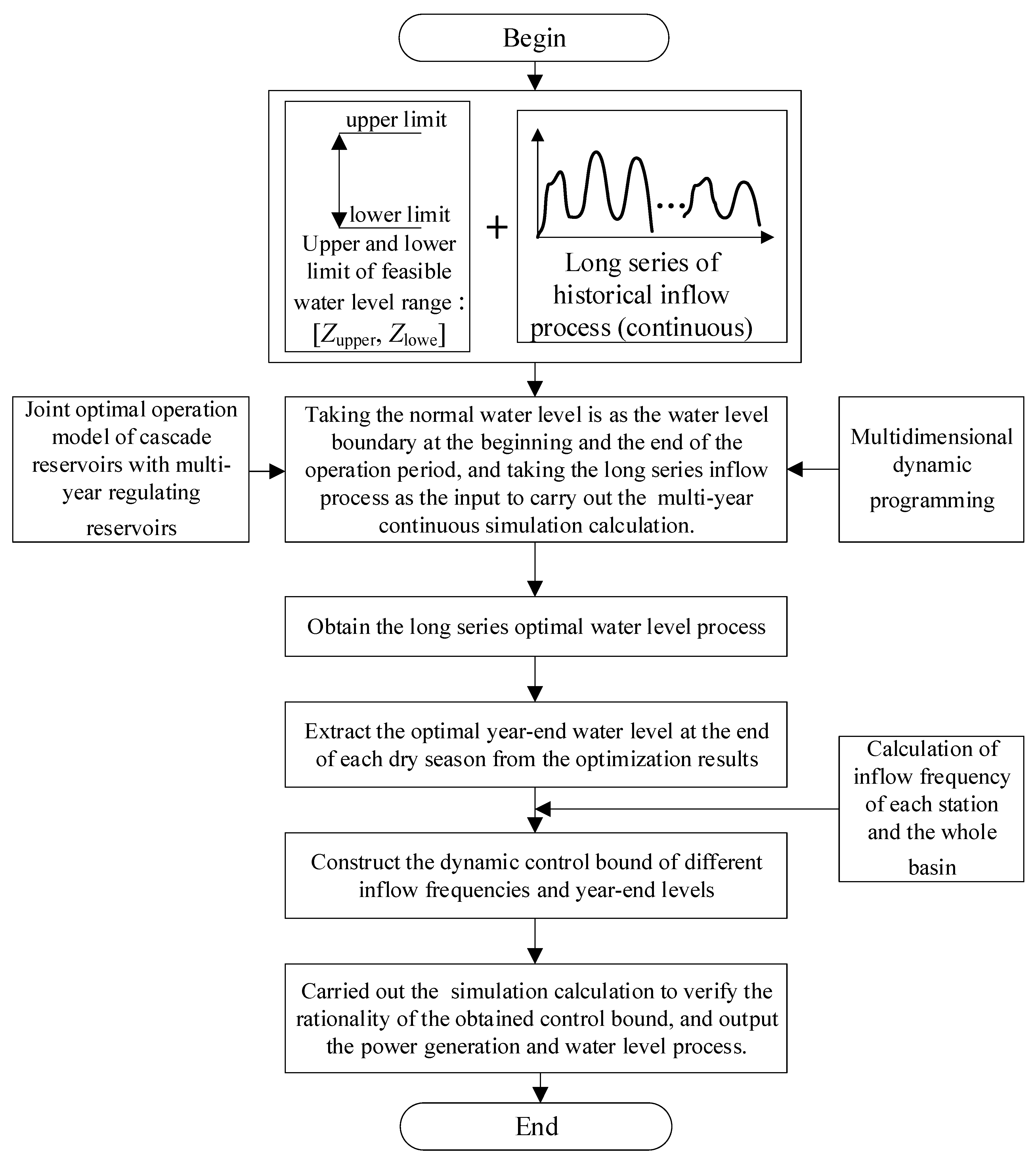
The overall flowchart of this method is shown in Figure 3.
In this method, the long series of inflows is used as the input, and the multidimensional DP algorithm is used for the continuous calculation, which can well consider the interannual inflow differences. However, inevitably, the calculation time is long. By this method, the dynamic control bound of the yearly drawdown level can be extracted according to the optimization results, that is, the control rule of the yearly drawdown level is expressed in the form of a dynamic control bound rather than a fixed value or function relation, which can well consider the inflow uncertainty. In addition, although it takes a long time to obtain the dynamic control bound by this method, considering that only the corresponding control rule (dynamic control bound) needs to be formulated here, rather than the real-time calculation, this method is used to study the optimal control of the yearly drawdown level in the case study of this paper.
3. Case Study
3.1. Study Area
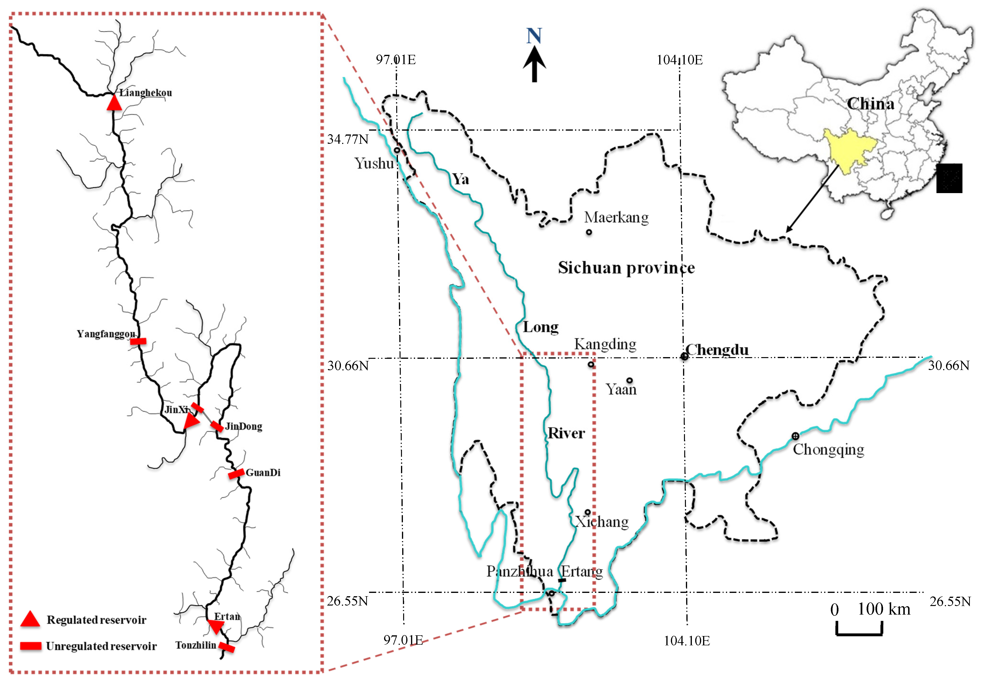
The Yalong River is the largest tributary of the Jinsha River in China, and its middle and lower reaches are currently the key river reaches for hydropower development in the mainstream of the river basin. There are seven hydropower stations: Lianghekou, Yangfanggou, Jinxi, Jindong, Guandi, Ertan and Tongzilin. Among them, the Lianghekou, Jinxi and Ertan reservoirs have regulation performances. Among them, the Lianghekou reservoir has an overyear regulation performance and is a control project for the middle and lower cascade hydropower stations, which has a great impact on the development of the cascade power stations in the entire basin [21].
After implementing scheduling, the cascade reservoirs in the middle and lower reaches can realize overyear regulation. The geographical location of the seven-reservoir cascade system in the Yalong River basin is shown in Figure 4, and the key parameters of each reservoir are shown in Table 1.
The data used in this study are 10-day inflow data from November 1957 to October 2018, a total of 61 years. In the calculation of the joint optimal scheduling model, the initial and final water levels of each reservoir with regulation performance are set as the normal water level, and the other reservoirs calculate and operate according to the water levels shown in Table 1.
3.2. Results and Analysis
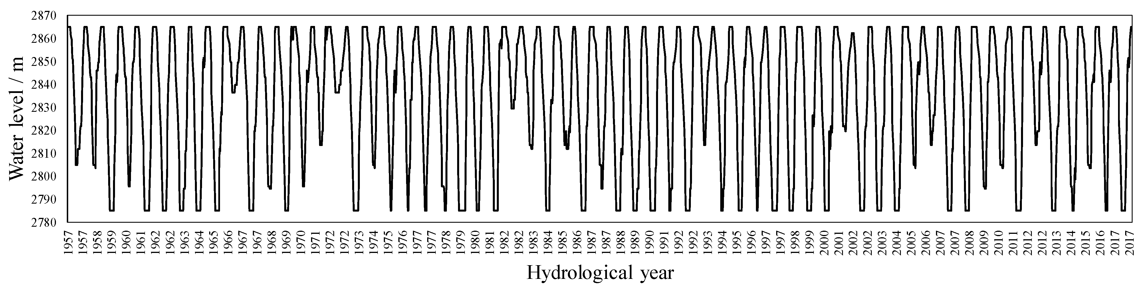
Through the proposed model and the relevant actual data in Section 3.1, the joint optimal scheduling model of this cascade system comprising seven reservoirs in the Yalong River basin can be established. Through the multidimensional DP method established in Section 2.2, the overyear optimal water level process of the Lianghekou reservoir can be obtained by taking 61 years of historical 10-day inflow data as the input, as shown in Figure 5. In the process of solving this model, 61 hydrological years are calculated continuously; that is to say, the spatial and interannual differences in the inflow are considered as a whole, so the spatial and temporal optimization are realized at the same time.
As shown in Figure 6, the operating water level of the Lianghekou reservoir fluctuates back and forth between the normal water level and dead water level, which is basically consistent with the periodicity of the inflow in a hydrological year. In addition, for most cases, the lowest water level is the dead water level of 2785 m; that is to say, in the long series simulation situation, the yearly drawdown level of this reservoir is mostly the dead water level, and a few cases are above the dead water level.
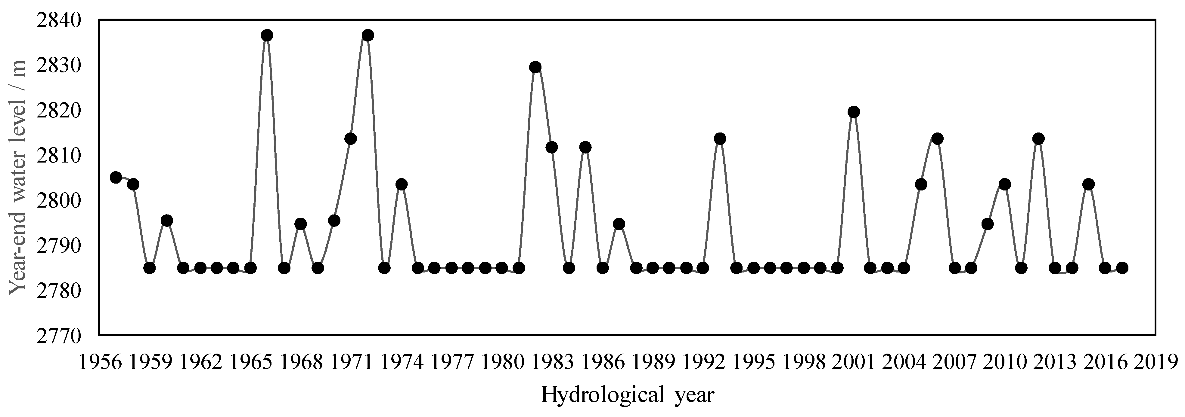
In order to further study the correlation between the inflow and the yearly drawdown level of each year, and to obtain a reasonable yearly drawdown level control rule, we extracted the optimal yearly drawdown level of the Lianghekou reservoir for each year, as shown in Figure 6.
As shown in Figure 6, the yearly drawdown level of the Lianghekou reservoir is 2875 m in most years, and the correlation between the yearly drawdown level and the year number is very weak; there are basically no rules to be found.
In view of the fact that the yearly drawdown level of an overyear regulation reservoir is strongly related to the amount of inflow water of current year, a correlation model between the yearly drawdown level of the Lianghekou reservoir and the inflow frequency can be established based on the optimization results, so as to judge the optimal yearly drawdown level according to the inflow frequency and realize dynamic control of the yearly drawdown level.
Here, only the hydrological station has the measured inflow data for the actual basin, and there is no actual inflow data that can represent the whole basin; for example, there are only the actual inflow data from the Lianghekou reservoir station, Jinxi reservoir station and Ertan reservoir station in this basin, and because of the large basin area, the inflow frequency of upstream and downstream stations must be different. Therefore, the selection of inflow series that is used to represent the inflow frequency of the whole basin has a great impact on the final results. In this paper, the inflow frequency representing the whole basin is calculated based on the least square principle and the inflow data of these three actual stations. Specifically, we set i as the index number of hydropower station and y as the index number of the hydrological year. The actual inflow frequency of each station in the yth year is Piy, which is obtained by its own frequency arrangement. If we want to obtain the optimal inflow process of the whole basin under a certain frequency Ps, it is equivalent to calculate the y corresponding to the smallest ey, which is shown in the following Formula (9):
The above method is used to deduce the best inflow process of the whole basin corresponding to the specific frequency Ps (a year). Conversely, a similar method can be used to derive the overall inflow frequency of each year for the river basin, such as the actual inflow frequency of the whole river basin in the year y.
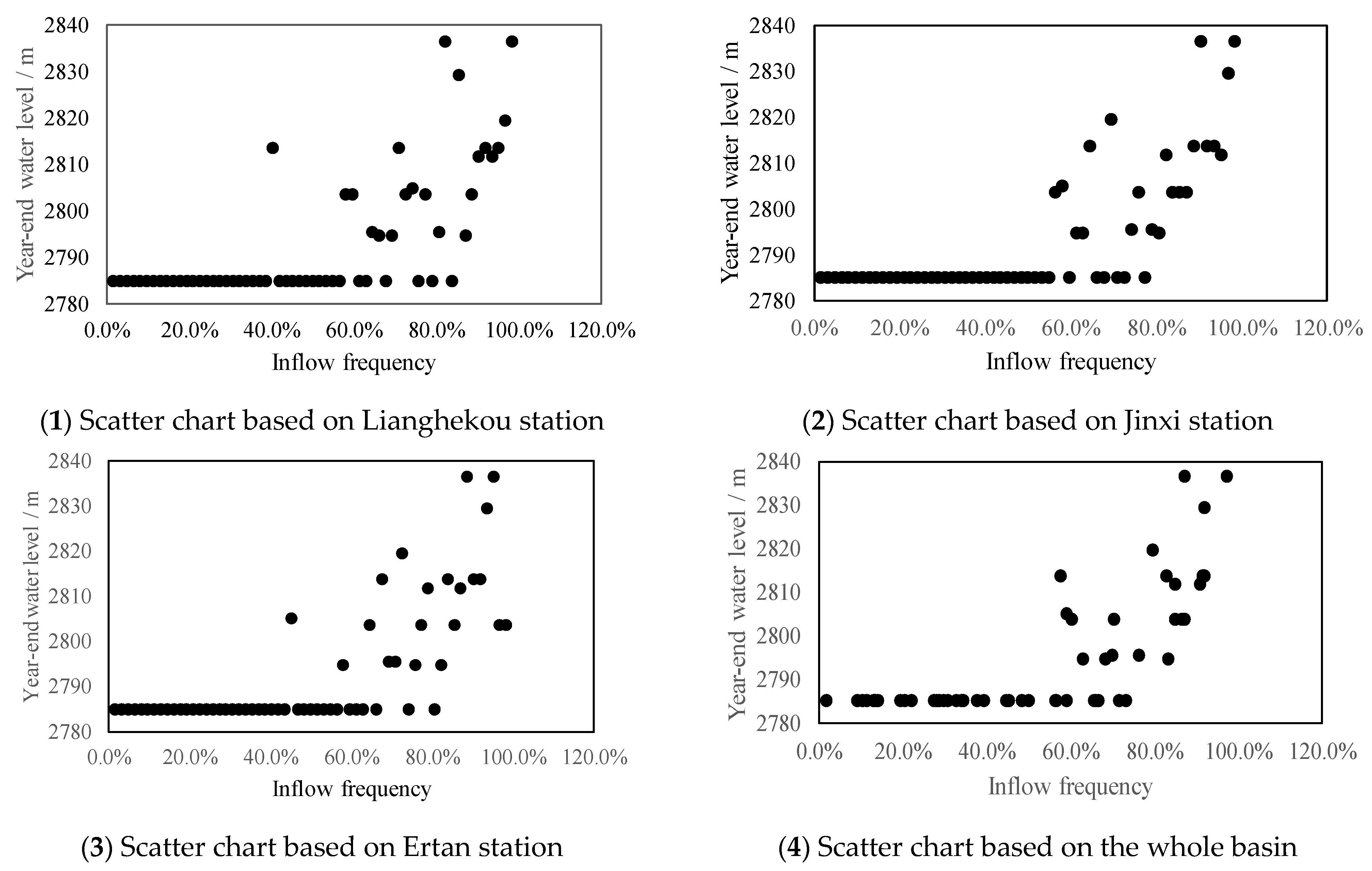
Taking the inflow frequencies of the Lianghekou reservoir station, Jinxi reservoir station and Ertan reservoir station as well as the overall inflow frequency of the whole basin as abscissa, and the optimal yearly drawdown level as an ordinate, the scatter relationships of the inflow frequency and the optimal yearly drawdown level are drawn, as shown in Figure 7.
It can be seen that in the above four cases, the scatters in cases (2) and (4) are relatively concentrated, and their correlation is good. The reason is that, in the second case, the Jinxi station is in the middle of the whole basin, and its inflow frequency can well represent the overall inflow of the river basin to a certain extent. In the fourth case, the overall inflow frequency is calculated by the least square principle based on the three actual stations, and it can also well represent the whole river basin. For cases (1) and (3), the station is upstream of the basin in case (1), and the station is located downstream of the basin in case (3), which both cannot represent the whole basin well. Therefore, we will take cases (2) and (4) as examples to calculate the dynamic control bound of the yearly drawdown level.
When the dynamic control bound is calculated based on the inflow data of the Jinxi station, as shown in the second case of Figure 8, the turning point of the scatter chart is 56.5%. The water level is the fixed value of 2785 m before this point, and it is a range after this point, which is the control bound we need to calculate. In order to obtain this range, based on the several most marginal points at the upper and lower boundaries of this range, the linear function relations are established respectively, and the dynamic control bound can be obtained by these two lines to form the upper and lower boundaries, as shown in Figure 8.
From Figure 9, it can be seen that the turning points of the upper boundary and the lower boundary are 56.5% and 77.4%, respectively. Therefore, the upper boundary of this dynamic control bound can be expressed as the following Formula (10):
Correspondingly, the lower boundary of this dynamic control bound can be expressed as the following Formula (11):
where Y represents the yearly drawdown level and I is the inflow frequency.
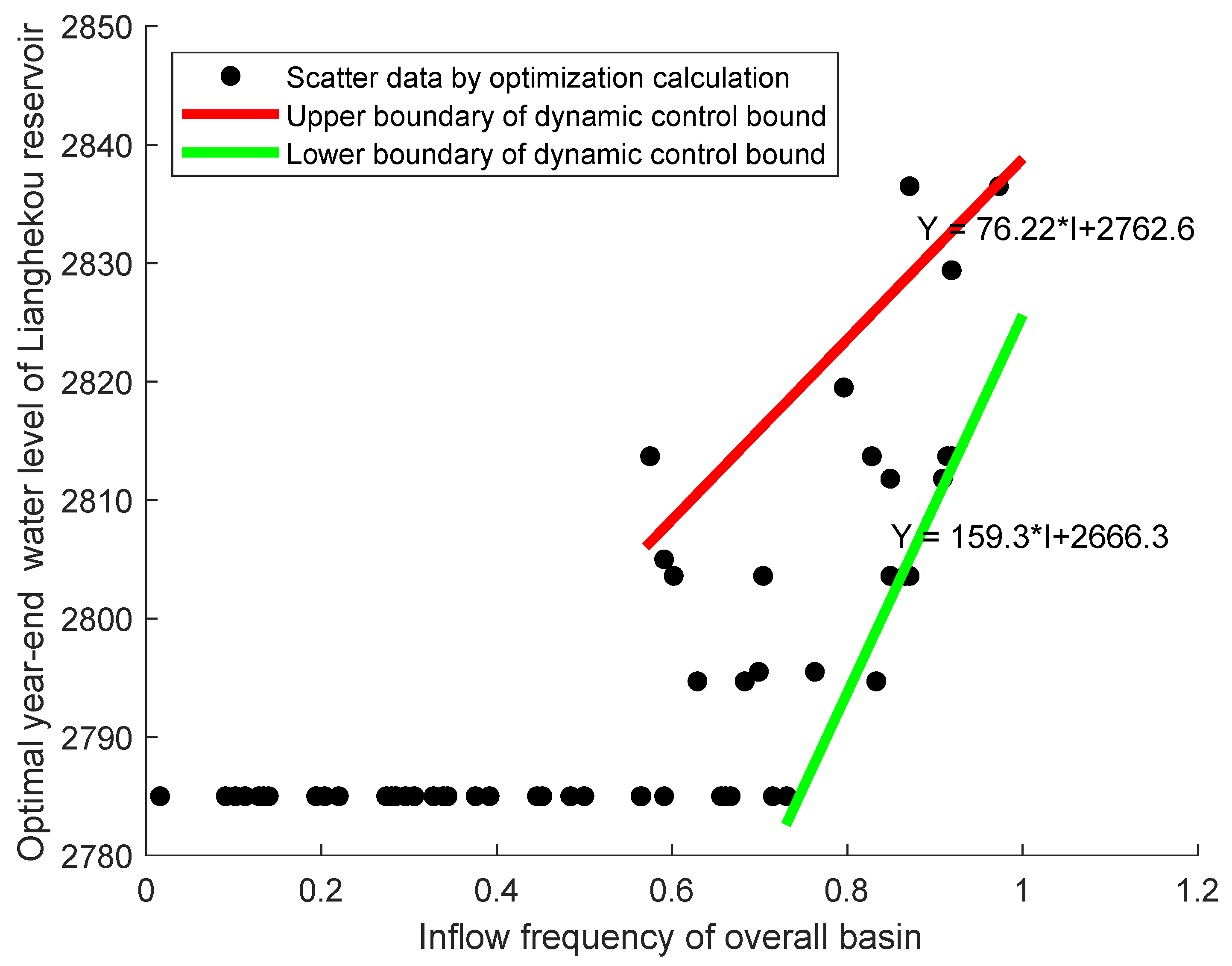
When the dynamic control bound is calculated based on the overall inflow frequency of the whole river basin, as shown in the fourth case of Figure 8, the turning point of the scatter chart is 57.5%. The water level is the fixed value of 2785 m before this point, and it is a range after this point, which is the control bound we need to calculate. Similarly, in order to obtain this range, based on the several most marginal points at the upper and lower boundaries of this range, the linear function relations are established respectively, and the dynamic control bound can be obtained by these two lines to form the upper and lower boundaries, as shown in Figure 9.
From Figure 10, it can be seen that the turning points of the upper boundary and the lower boundary are 57.5% and 73.1%, respectively. Therefore, the upper boundary of this dynamic control bound can be expressed as the following Formula (12):
Correspondingly, the lower boundary of this dynamic control bound can be expressed as the following Formula (13):
After obtaining the above dynamic control bounds of the yearly drawdown level expressed by subsection functions, in order to analyze and compare them rationally, it is necessary to simulate and calculate the total power generation of the cascade system in the following cases: the upper boundary of the dynamic control bound, the lower boundary of the dynamic control bound, the mean value of the dynamic control bound and the original fixed yearly drawdown level. In the simulation calculation of the first three cases, in order to ensure the water balance between years, overyear continuous calculation is required, and the yearly drawdown level value of each year is controlled by the established control rules.
First of all, the optimal results under the fixed water level are provided, as shown in Table 2. Within the feasible range, a series of discrete water levels is obtained by discretizing, and a long series of historical inflow data is taken as the input of the model. The simulation results are as follows.
As shown in Table 2, the maximum power generation of the cascade system is 100.580 billion kWh under the fixed water level mode, and the corresponding optimal yearly drawdown level is 2785 m, which is the dead water level of this reservoir. From this point of view, if the fixed water level mode is to be used for the actual scheduling, the dead water level is the best yearly drawdown level for this overyear regulation reservoir. That is, the reservoir only has annual regulation performance at this time.
Secondly, the calculation results of the dynamic control bound of the yearly drawdown level under three different control modes are provided, as shown in Table 3. These three control modes are as follows: (1) the upper boundary of the control bound is used as the control rule in the calculation; (2) the lower boundary of the control bound is used as the control rule in the calculation; and (3) the mean value of the control bound is used as the control rule in the calculation. For convenience of comparison, this table also provides the optimal calculation results based on the fixed-yearly-drawdown-level mode and multidimensional DP. It can be seen from Table 2 that the annual total power generation of the fixed water level mode is 100.58 billion kWh, and the percentage in Table 3 is the increase in the total annual power generation under different scheduling rules compared to the fixed water level mode.
As shown in Table 3, for the power generation results of the dynamic control bound constructed based on the inflow series of the Jinxi station, the differences among the upper boundary, lower boundary and mean value are not significant, and the maximum difference is only 0.110 billion kWh. Similarly, for the power generation results of the dynamic control bound constructed based on the overall inflow series of the river basin, the differences among the upper boundary, lower boundary and mean value are not significant either, and the maximum difference is only 0.107 billion kWh. This shows that the control result of the yearly drawdown level is less fluctuant according to the constructed dynamic control bound, which can well deal with the impact of inflow uncertainty on the scheduling results. Thus, the rationality of the constructed dynamic control bound of yearly drawdown level is well verified.
Relatively speaking, from the results of power generation, the dynamic control bound constructed based on the overall inflow of the river basin is slightly better than that based on the inflow of the Jinxi station. In all the three cases where the upper boundary, lower boundary and mean value are used as the control rules, the power generation of the former is 0.01% higher than that of the latter.
In addition, from the comparison between the results of the fixed-yearly-drawdown-level control mode and the results of the optimal calculation by multidimensional DP, the maximum lifting space of control optimization of the yearly drawdown level is about 0.93%. In this paper, by building a dynamic control mode for the yearly drawdown level, 0.59~0.71% of 0.93% can be realized; that is to say, 63.4~76.3% of the benefits of the lifting space of yearly drawdown level optimization can be realized by the dynamic control bound, which has a very remarkable effect.
Under different control rules, the overyear average water level processes of the Lianghekou reservoir are shown in Figure 10.
It can be seen that under different calculation methods or control modes, the overyear average water level processes of the Lianghekou reservoir show strong regularity, especially for the water level at the end of the dry season (end of the hydrological year). The law is that the water level calculated by the multidimensional DP method is in the middle, the water level calculated by the upper and lower boundaries of the dynamic control bounds obtained through the inflow of the Jinxi station and the whole basin are located on the two sides of the optimal value of multidimensional DP, and the water level calculated by the upper and lower boundaries of the dynamic control bound obtained by the inflow of the whole basin is closer to the optimal value. This law is consistent with the power generation results in Table 3.
In addition, the water levels calculated from the mean value of the Jinxi station and the whole-basin dynamic control bounds are not significantly different from the results of multidimensional DP optimization, and the difference in power generation is only 0.007 billion kWh (101.290–101.283). In the low-water-level period, the water-level processes of these two control rules basically coincide. In the high-water-level period, the water-level results are basically the same too, but they are all below the optimal water level obtained by the multidimensional DP method, so the total power generation is lower than the optimal value of multidimensional DP (101.290 < 101.520, 101.283 < 101.520).
4. Conclusions
In order to balance the spatial and interannual distribution differences of the inflow of a river basin reasonably and improve the total power generation of a cascade reservoir system, based on the joint scheduling model of cascade reservoirs and a multidimensional DP algorithm, this paper studies the yearly drawdown level optimization problem of an overyear regulation reservoir considering the influence of inflow uncertainty. A feasible technical route for this problem is proposed, and the advantages and disadvantages of the this technical routes are analyzed. Taking the cascade system that contains seven reservoirs in the Yalong River basin as an example, this technical route is tested and verified. The dynamic control bounds of the yearly drawdown level of the Lianghekou reservoir under two selected inflow series are constructed, the simulation calculations and a detailed comparative analysis are carried out, and the following conclusions are obtained:
- (1)
- The inflow series of the station in the middle of the basin and the calculated overall inflow series can both well represent the inflow situation of the whole basin. In these two cases, the relationship between the inflow frequency and the scatter points of the yearly drawdown level is relatively centralized and stable. The results of the inflow series of stations that are located in the upper and lower parts of the basin are relatively poor.
- (2)
- Under the control mode of the fixed yearly drawdown level, the maximum annual average power generation of the cascade system is 100.580 billion kWh, and the corresponding optimal yearly drawdown level is 2785 m, which is the dead water level. That is to say, if the yearly drawdown level is to be fixed, the dead water level is the best for the Lianghekou reservoir.
- (3)
- For the dynamic control bounds constructed by the two selected inflow series, the results calculated from their upper boundaries, lower boundaries and mean values are not significant, and their maximum differences are 0.110 billion kWh and 0.107 billion kWh, respectively. This shows that the results of the dynamic control bounds constructed by the two selected inflow series both have little fluctuation, which can well cope with the impact of inflow uncertainty on scheduling results.
- (4)
- The dynamic control bound constructed based on the overall inflow of the river basin is slightly better than that based on the inflow of the Jinxi station. In all the three cases where the upper boundary, lower boundary and mean value are used as the control rules, the power generation of the former is 0.01% higher than that of the latter.
- (5)
- By constructing a dynamic control mode of the yearly drawdown level, 63.4%~76.3% of the benefits of the lifting space of yearly drawdown level optimization can be realized by the dynamic control bound proposed in this paper, which has a very remarkable effect.
Author Contributions
Z.C.: data curation, formal analysis and writing—review and editing; Z.J.: conceptualization, funding acquisition and methodology; X.Y.: data curation and funding acquisition. All authors have read and agreed to the published version of the manuscript.
Funding
This study was financially supported by the National Key R&D Program of China (2021YFC3200400), the Natural Science Foundation of China (52179016) and the Natural Science Foundation of Hubei Province (2021CFB597).
Data Availability Statement
Data, models and code that support the findings of this study are available from the corresponding author upon reasonable request.
Conflicts of Interest
The authors declare no conflict of interest.
Nomenclature
We define following parameters, variables and indices.
| Db: | the index of beginning-state variables of downstream reservoirs. |
| De: | the index of end-state variables of downstream reservoirs. |
| E: | power generation over the whole scheduling period (kWh). |
| Epti: | the evaporation capacity of the ith reservoir in the tth stage (m3/s). |
| f t*(V): | the sum of optimal outputs from the present stage t to the last stage T. |
| Hti: | the average water head of the ith hydropower station in the tth stage (m). |
| Iti: | the average interval inflow of the ith reservoir in the tth stage (m3/s). |
| Ki: | the output coefficient of the ith hydropower station. |
| Nti: | the output of the ith hydropower station in the tth stage (kW). |
| Nit,min: | the lower limit of Nit. |
| Nit,max: | the upper limit of Nit. |
| Nt(Vt−1,Qt): | the total output of the tth stage. |
| qti: | the outflow through the turbines of the ith reservoir in the tth stage (m3/s). |
| Qit: | the average discharge of the ith reservoir in the tth stage (m3/s). |
| Qt: | the discharge flow determined by Vt−1 and Vt. |
| Qt = (Qt1, Qt2, …, Qt n)’: | the decision variable vector. |
| Qit,min: | the lower limit of Qit. |
| Qit,max: | the upper limit of Qit. |
| T: | the total number of stages over the whole scheduling period. |
| Dt: | a set of feasible decisions that satisfy the constraints of the reservoir. |
| Δt: | the duration of a stage (h). |
| Ub: | the index of beginning-state variables of upstream reservoirs. |
| Ue: | the index of end-state variables of upstream reservoirs. |
| Vit: | the storage volume of the ith reservoir in the tth stage (m3). |
| Vt: | the storage state at the beginning of the stage t. |
| Vit,min: | the lower limit of Vit. |
| Vit,max: | the upper limit of Vit. |
| V0i: | the storage volume of the ith reservoir at the beginning of the first stage. |
| Vbi: | the storage volume of the ith reservoir at the beginning of the whole scheduling period. |
| VTi: | the storage volume of the ith reservoir at the end of the Tth stage. |
| Vei: | the storage volume of the ith reservoir at the end of the whole scheduling period. |
| Vt−1 = (Vt−11, Vt−12, …, Vt−1n)’: | the state variable vector. Vt1, Vt2, and Vt3 are discretized, i.e., (Vt1,1, Vt1,2, …, Vt1,M), (Vt2,1, Vt2,2, …, Vt2,M) and (Vt3,1, Vt3,2, …, Vt3,M). |
| : | |
| : | the optimal cumulative output of a storage volume combination VT at the end of the Tth stage (kW). |
| Wti: | the average discharge of abandoned water of the ith reservoir in the tth stage (m3/s). |
References
- Siddiqui, O.; Dincer, I. Comparative assessment of the environmental impacts of nuclear, wind and hydro-electric power plants in Ontario: A life cycle assessment. J. Clean. Prod. 2017, 164, 848–860. [Google Scholar] [CrossRef]
- Jurasz, J.; Mikulik, J.; Krzywda, M.; Ciapała, B.; Janowski, M. Integrating a wind- and solar-powered hybrid to the power system by coupling it with a hydroelectric power station with pumping installation. Energy 2018, 144, 549–563. [Google Scholar]
- Lu, S.; Shang, Y.; Li, W.; Peng, Y.; Wu, X. Economic benefit analysis of joint operation of cascaded reservoirs. J. Clean. Prod. 2018, 179, 731–737. [Google Scholar] [CrossRef]
- Bertone, E.; O’ Halloran, K.; Stewart, R.A.; de Oliveira, G.F. Medium-term storage volume prediction for optimum reservoir management: A hybrid data-driven approach. J. Clean. Prod. 2017, 154, 353–365. [Google Scholar]
- Allawi, M.F.; Jaafar, O.; Mohamad Hamzah, F.; El-Shafie, A. Novel reservoir system simulation procedure for gap minimization between water supply and demand. J. Clean. Prod. 2019, 206, 928–943. [Google Scholar] [CrossRef]
- Arena, C.; Cannarozzo, M.; Mazzola, M.R. Exploring the Potential and the Boundaries of the Rolling Horizon Technique for the Management of Reservoir Systems with over-Year Behaviour. Water Resour. Manag. 2017, 31, 867–884. [Google Scholar] [CrossRef]
- Guo, X.; Chen, J.; Ma, G. Research on yearly drawdown level of overyear regulating storage reservoir for timed power tariff. J. Hydroelectr. Eng. 2004, 23, 27. [Google Scholar]
- Yuan, W.; Wang, F. Study on year-end water level of overyear regulating storage reservoir in power market. J. Hydroelectr. Eng. 2012, 31, 94–98. [Google Scholar]
- Zhang, Y.; Jiang, Z.; Ji, C.; Sun, P. Contrastive analysis of three parallel modes in multi-dimensional dynamic programming and its application in cascade reservoirs operation. J. Hydrol. 2015, 529, 22–34. [Google Scholar]
- Wang, J.; Huang, W.; Ma, G.; Wang, Y. Determining the optimal year-end water level of a overyear regulating storage reservoir: A case study. Water Sci. Technol. Water Supply 2016, 16, 284–294. [Google Scholar] [CrossRef]
- Liu, J.; Huang, C.; Zeng, G. Comparative analysis of year-end water level determining methods for cascade carryover storage reservoirs. IOP Conf. Ser. Earth Environ. Sci. 2017, 82, 1–8. [Google Scholar]
- Ehteram, M.; Karami, H.; Mousavi, S.F.; Farzin, S.; Kisi, O. Optimization of energy management and conversion in the multi-reservoir systems based on evolutionary algorithms. J. Clean. Prod. 2017, 168, 1132–1142. [Google Scholar]
- Jiang, Z.; Liu, P.; Ji, C.; Zhang, H.; Chen, Y. Ecological flow considered multi-Objective storage energy operation chart optimization of large-scale mixed reservoirs. J. Hydrol. 2019, 577, 123949. [Google Scholar] [CrossRef]
- Li, R.; Jiang, Z.; Li, A.; Yu, S.; Ji, C. An improved shuffled frog leaping algorithm and its application in the optimization of cascade reservoir operation. Hydrol. Sci. J. 2018, 63, 15–16. [Google Scholar] [CrossRef]
- Liu, S.; Xie, Y.; Fang, H.; Huang, Q.; Huang, S.; Wang, J.; Li, Z. Impacts of inflow variations on the long term operation of a multi-hydropower-reservoir system and a strategy for determining the adaptable operation rule. Water Resour. Manag. 2020, 34, 1649–1671. [Google Scholar] [CrossRef]
- Fang, W.; Huang, S.Z.; Ren, K.; Huang, Q.; Huang, G.H.; Cheng, G.H.; Li, K.L. Examining the applicability of different sampling techniques in the development of decomposition-based streamflow forecasting models. J. Hydrol. 2019, 568, 534–550. [Google Scholar]
- Goulter, I.C.; Tai, F.-K. Practical implications in the use of stochastic dynamic programming for reservoir operation. JAWRA J. Am. Water Resour. Assoc. 2007, 21, 65–74. [Google Scholar] [CrossRef]
- Adib, A.; Samandizadeh, M.A. Comparison ability of GA and DP methods for optimization of released water from reservoir dam based on produced different scenarios by Markov chain method. Int. J. Optim. Civ. Eng. 2016, 6, 43–62. [Google Scholar]
- Jiang, Z.; Ji, C.; Qin, H.; Feng, Z. Multi-stage progressive optimality algorithm and its application in energy storage operation chart optimization of cascade reservoirs. Energy 2018, 148, 309–323. [Google Scholar]
- Zhang, Z.; Zhang, S.; Geng, S.; Jiang, Y.; Li, H.; Zhang, D. Application of decision trees to the determination of the yearly drawdown level of a carryover storage reservoir based on the iterative dichotomizer 3. Int. J. Electr. Power Energy Syst. 2015, 64, 375–383. [Google Scholar]
- Jiang, Z.; Tang, Z.; Liu, Y.; Chen, Y.; Feng, Z.; Xu, Y.; Zhang, H. Area moment and error basedforecasting difficulty and its application ininflow forecasting level evaluation. Water Resour. Manag. 2019, 33, 4553–4568. [Google Scholar] [CrossRef]
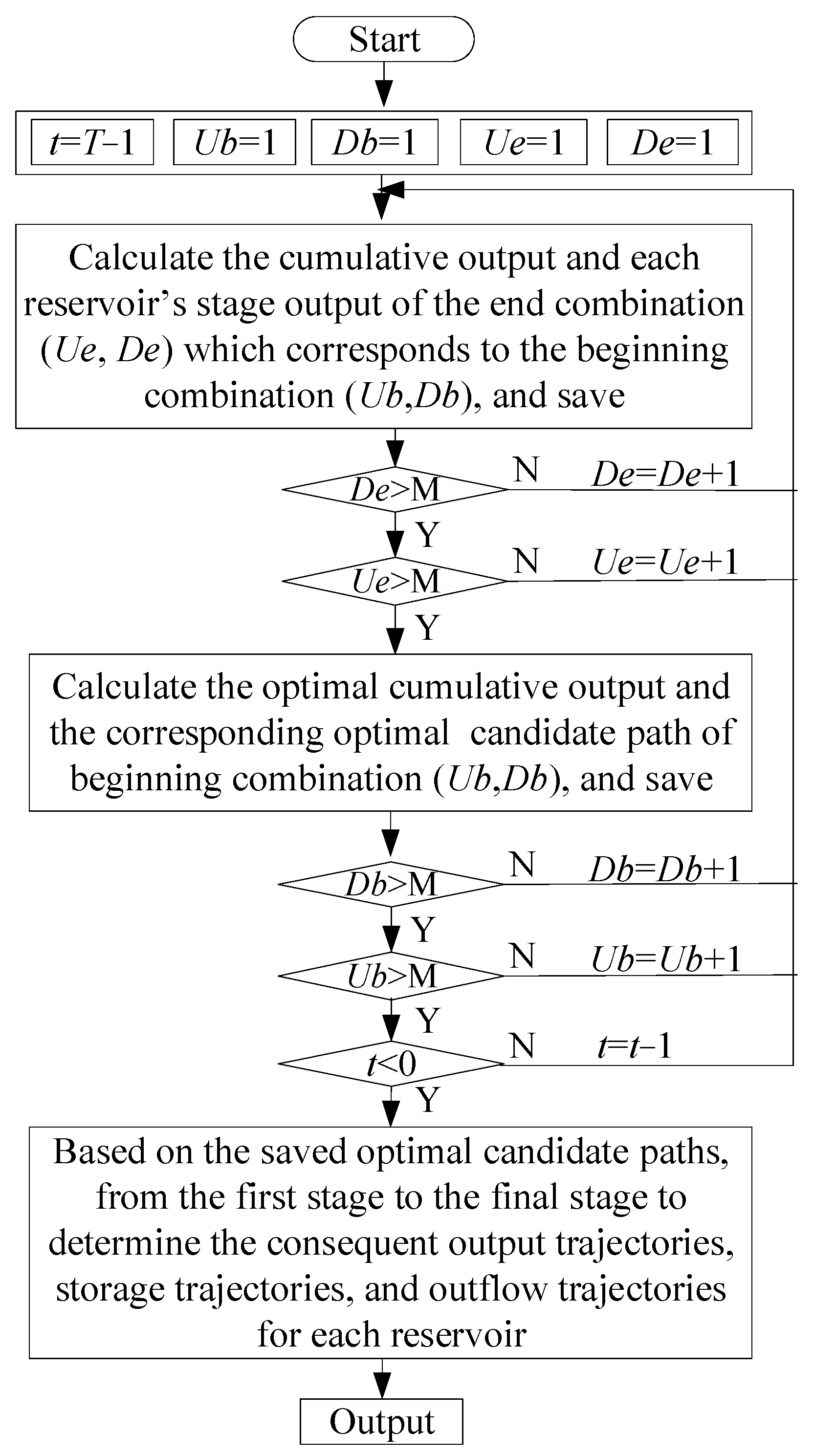
Figure 1.
Flowchart of multidimensional DP in solving joint optimal scheduling of cascade reservoirs.
Figure 1.
Flowchart of multidimensional DP in solving joint optimal scheduling of cascade reservoirs.

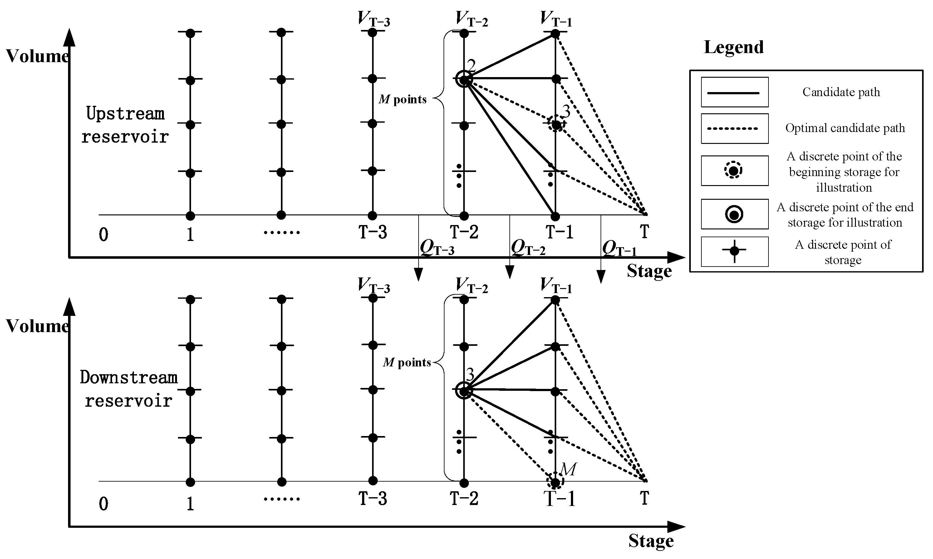
Figure 2.
Reverse recursion procedure of multidimensional DP for joint optimal scheduling of cascade reservoirs.
Figure 2.
Reverse recursion procedure of multidimensional DP for joint optimal scheduling of cascade reservoirs.

Figure 3.
Optimal control scheme of yearly drawdown level of overyear regulation reservoir: dynamic control bound model.
Figure 3.
Optimal control scheme of yearly drawdown level of overyear regulation reservoir: dynamic control bound model.

Figure 4.
Geographical location of the seven-reservoir cascade system.

Figure 5.
Overyear optimal water level process of Lianghekou reservoir based on multidimensional DP.
Figure 5.
Overyear optimal water level process of Lianghekou reservoir based on multidimensional DP.

Figure 6.
Variation of the optimal yearly drawdown level of the Lianghekou reservoir in each year.

Figure 7.
Scatter charts of inflow frequency and yearly drawdown level of Lianghekou reservoir with different incoming flow frequencies as references.
Figure 7.
Scatter charts of inflow frequency and yearly drawdown level of Lianghekou reservoir with different incoming flow frequencies as references.

Figure 8.
Dynamic control bound of yearly drawdown level constructed by inflow series of Jinxi station.
Figure 8.
Dynamic control bound of yearly drawdown level constructed by inflow series of Jinxi station.

Figure 9.
Dynamic control bound of yearly drawdown level constructed by the overall inflow series of the whole basin.
Figure 9.
Dynamic control bound of yearly drawdown level constructed by the overall inflow series of the whole basin.

Figure 10.
Overyear average water level processes of Lianghekou reservoir under different control rules.
Figure 10.
Overyear average water level processes of Lianghekou reservoir under different control rules.


Table 1.
The key parameters of the seven reservoirs.
| Item | Unit | Lianghekou | Yangfanggou | Jinxi | Jindong | Guandi | Ertan | Tongzilin |
|---|---|---|---|---|---|---|---|---|
| Normal level | m | 2865 | 2088 | 1880 | 1646 | 1330 | 1200 | 1015 |
| Dead level | m | 2785 | 2094 | 1800 | 1640 | 1321 | 1155 | 1010 |
| Annual average runoff | m3/s | 664 | 896 | 1200 | 1220 | 1430 | 1670 | 1928 |
| Mean annual precipitation | mm | 897 | None | None | 932 | 1077 | 1038 | 1040 |
| Temperature | °C | 10.9 | 13.7 | 13.7 | 13.7 | 18.6 | 19.8 | 19.7 |
| Flood control level | m | 2845.9 | None | 1859 | None | None | 1190 | None |
| Regulation performance | --- | Overyear | Daily | Yearly | Daily | Daily | Seasonal | Daily |
| Range of operating water level in dry season | m | [2845.9, 2865] | 2092 | [1859, 1880] | 1644 | 1328 | [1190, 1200] | 1013.5 |
| Range of operating water level in flood season | m | [2785, 2865] | 2092 | [1800, 1880] | 1644 | 1328 | [1155, 1200] | 1013.5 |
Table 2.
Annual power generation of cascade system under different yearly drawdown levels of Lianghekou reservoir.
Table 2.
Annual power generation of cascade system under different yearly drawdown levels of Lianghekou reservoir.
| Yearly Drawdown Level/m | Total Power Generation/Billion kWh |
|---|---|
| 2785 | 100.58 |
| 2790 | 100.55 |
| 2795 | 100.49 |
| 2800 | 100.43 |
| 2805 | 100.30 |
| 2810 | 100.16 |
| 2815 | 99.95 |
| 2820 | 99.72 |
| 2825 | 99.43 |
| 2830 | 99.08 |
| 2835 | 98.64 |
| 2840 | 98.10 |
| 2845 | 97.37 |
Table 3.
Power generation results under the three control modes based on the obtained dynamic control bound.
Table 3.
Power generation results under the three control modes based on the obtained dynamic control bound.
| Computation Method | Total Power Generation/Billion kWh | Increment Compared to Fixed Water Level Mode |
|---|---|---|
| Upper boundary of the dynamic control bound constructed based on Jinxi inflow series | 101.255 | 0.67% |
| Lower boundary of the dynamic control bound constructed based on Jinxi inflow series | 101.173 | 0.59% |
| Mean value of the dynamic control bound constructed based on Jinxi inflow series | 101.283 | 0.70% |
| Upper boundary of the dynamic control bound constructed based on the overall inflow series | 101.267 | 0.68% |
| Lower boundary of the dynamic control bound constructed based on the overall inflow series | 101.183 | 0.60% |
| Mean value of the dynamic control bound constructed based on the overall inflow series | 101.290 | 0.71% |
| Fixed yearly drawdown level (determined by discretized water levels) | 100.580 | 0.00% |
| Optimal calculation results based on multidimensional DP | 101.520 | 0.93% |
Disclaimer/Publisher’s Note: The statements, opinions and data contained in all publications are solely those of the individual author(s) and contributor(s) and not of MDPI and/or the editor(s). MDPI and/or the editor(s) disclaim responsibility for any injury to people or property resulting from any ideas, methods, instructions or products referred to in the content. |
© 2023 by the authors. Licensee MDPI, Basel, Switzerland. This article is an open access article distributed under the terms and conditions of the Creative Commons Attribution (CC BY) license (https://creativecommons.org/licenses/by/4.0/).
Share and Cite
MDPI and ACS Style
Chang, Z.; Jiang, Z.; Yuan, X. Dynamic Control of Yearly Drawdown Level of Overyear Regulation Reservoir in Cascade System. Water 2023, 15, 665. https://doi.org/10.3390/w15040665
AMA Style
Chang Z, Jiang Z, Yuan X. Dynamic Control of Yearly Drawdown Level of Overyear Regulation Reservoir in Cascade System. Water. 2023; 15(4):665. https://doi.org/10.3390/w15040665
Chicago/Turabian StyleChang, Zongye, Zhiqiang Jiang, and Xiaohui Yuan. 2023. "Dynamic Control of Yearly Drawdown Level of Overyear Regulation Reservoir in Cascade System" Water 15, no. 4: 665. https://doi.org/10.3390/w15040665
Note that from the first issue of 2016, this journal uses article numbers instead of page numbers. See further details here.