Predicting Higher Heating Value of Sewage Sludges via Artificial Neural Network Based on Proximate and Ultimate Analyses

Abstract

The higher heating value (HHV) was an important factor for measuring the energy recovery price of sewage sludge, which was commonly determined by oxygen bomb calorimeter; however, there were problems of time consuming and high measurement cost. In this study, a back-propagation neural network (BPNN) model based on proximate and ultimate combination analysis was developed to predict the HHV of sewage sludge and the accuracy of the model was illustrated using statistical analysis. The results showed that the BPNN model had good accuracy, with a regression coefficient of 0.979 and 0.975 for the training and test groups, respectively. Several previously proposed linear models for predicting the HHV of sewage sludge were selected for comparison. The results showed that the BPNN model was the best among all models with the highest regression coefficient (0.975) and the lowest mean absolute deviation (0.385).

1. Introduction

Sewage sludge is composed of both the original solids in the wastewater and the solids produced by the wastewater treatment [1,2,3]. The treated sewage sludge can be maintained in a stable state, thus reducing the negative impact on the environment [4]. It has been pointed out that sewage sludge contains a large amount of organic matter, such as cellulose, lignin, fat and protein [5,6,7,8]. After drying treatment, water content in sewage sludge can reduce to less than 10% with a heating value above 11 MJ/kg, which indicated that sewage sludge had a high energy recovery value [9,10].

The main methods of energy recovery from sewage sludge are biochemical and thermochemical [11,12,13], where biochemical methods include anaerobic digestion [14] and gasification [15], while thermochemical methods include incineration [16,17] and pyrolysis [18]. In the reaction process, the higher heating value (HHV) of sewage sludge is the most important factor used to measure its energy recovery potential and to determine which method to use to recover its energy [19,20]. The HHV of the fuel is the amount of heat generated per unit mass of body mass when it is completely burned and it includes the latent heat of vaporization of water vapor generated when the fuel is burned. As a potential biofuel, the HHV of sewage sludge determines its final energy output [21].

The oxygen bomb calorimeter is the most common method for the measurement of HHV. Although this method is reliable, it has the problems of being time-consuming and having a high measurement cost [22,23]. In order to overcome the mentioned shortcomings, different type of linear models were developed for predicting HHV. The previous literature reported that a model for multiple linear regression analysis using the least-squares method was developed for predicting the HHV of lignocellulose and charcoal based on proximate analysis [24]. Furthermore, Kathiravale et al. [25] established a linear model based on proximate analysis or ultimate analysis to predict the HHV of municipal solid waste by regression analysis. This linear model based on regression analysis was also used to predict the HHV of livestock manure and mixtures [26]. As proximate analysis (moisture, volatile matter, fixed carbon and ash) and ultimate analysis (carbon, hydrogen, oxygen, nitrogen and sulfur) were the main features of biofuels, HHV can be calculated on this basis by linear regression, thus replacing the oxygen bomb calorimeter. However, sewage sludge has shown non-linear relationships between HHV and ultimate analysis [27]. Among them, nitrogen, sulfur and oxygen show clear non-linear relationships in addition to fixed carbon in the proximate analysis. Similar irrelevance was found in predicting the HHV of biomass [28], and Ghugare et al. [23] demonstrated that linear models were not the best method to use for predicting HHV. Therefore, linear models may not be the best choice for predicting the HHV of sewage sludge, and non-linear models are needed.

As a non-linear model, the artificial neural network (ANN) model was considered to be the most reliable and convenient for this purpose [29]. Unlike traditional linear models, ANNs are one of the most common methods for analyzing the relationships between linear and non-linear data [30,31]. Kapetanakis et al. [32] developed a multilayer perceptron artificial neural network model to predict the HHV of sewage sludge hydrate, and the results showed that the model had high accuracy in predicting the results. Gülce Çakman et al. [33] developed an ANN model based on a back-propagation algorithm to predict the HHV of biochars and compared it with eight linear models, and the results showed that the ANN model performed far better than the linear models. MortezaTaki et al. [34] demonstrated four different ANN models to predict the HHV of municipal solid waste and the results showed that all the ANN models had regression coefficients above 0.92. ANN models generally perform better in predicting HHV than linear models, as ANNs work as a network stimulated like a nervous system and can be continuously trained to improve the accuracy of the prediction [35]. Currently, most studies have used linear models to predict the HHV of sewage sludge, but the errors in the obtained predictions were relatively large and could not replace the oxygen bomb calorimeter. The ANN model showed good performance when applied to materials (biomass, municipal solid waste, etc.) similar to sewage sludge and may also be suitable for applications with sewage sludge, which requires further study.

Based on a review of the previous literature, it was found that ANN models demonstrate the best performance in predicting HHV, but no reports have been seen of building ANN models to predict the HHV of sewage sludge. The focus of this study was to develop a back-propagation neural network (BPNN) model to predict the HHV of sewage sludge based on proximate and ultimate analyses. The accuracy of the BPNN model was verified by experimentally determined HHV, then compared with several published linear models used to predict the HHV of sewage sludge. The objective of this study was to develop an accurate model to predict the HHV of sewage sludge without an oxygen bomb calorimeter and to provide a basis for selecting a method to recover energy from sewage sludge.

2. Materials and Methods

2.1. Source of Sample

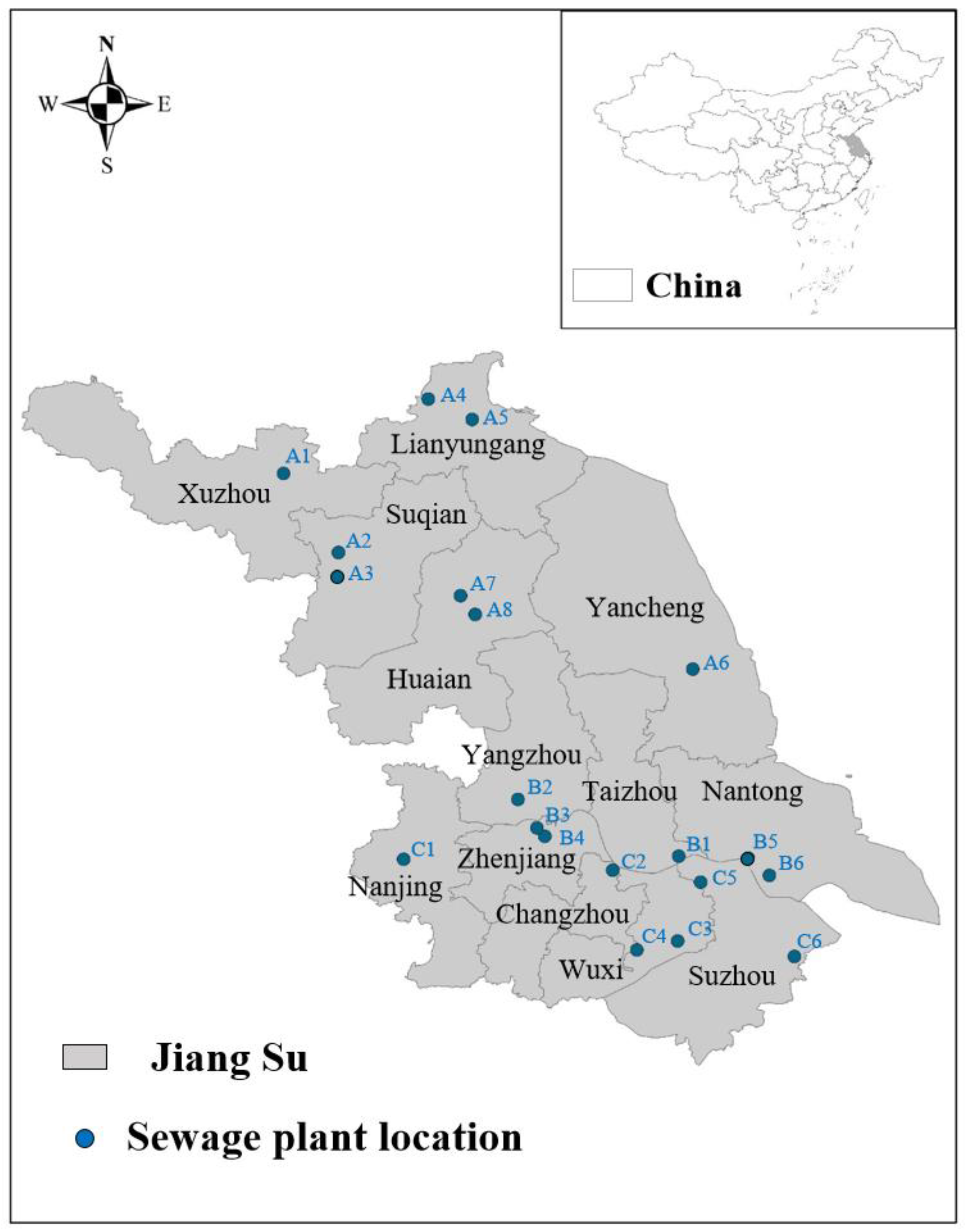
The sewage sludge samples used in this study were collected from 20 different wastewater treatment plants in different regions of Jiangsu Province, China. The sample numbers A, B and C represent the samples from the north, middle and south of Jiangsu Province, respectively. The specific locations of the wastewater treatment plants are shown in Figure 1.

All wastewater treatment plants treat domestic wastewater as the main target. Additionally, the biochemical treatment processes of wastewater treatment plants were mainly divided into three categories: (1) Anaerobic/Anoxic/Oxic (A/A/O) and its deformation process, including the inverted A/A/O process and the UCT process, etc.; (2) Oxidation Ditch process, including multi-trench alternating oxidation ditch and Orbal oxidation ditch, etc.; and (3) Sequencing batch reactor-activated sludge process and its deformation process, including CASS and UNITANK processes, etc.

2.2. Sample Preparation

Sewage sludge was sampled at multiple points on the conveyor belt of the dewatering machine and then mixed into one sample. If multiple machines were working at the same time, a portion of the sewage sludge was taken from each machine, then mixed into one sample. Each sample size was approximately 200 g. Sampling was repeated six times for each treatment plant at two month intervals from December 2021 to October 2022, resulting in a total of 120 sewage sludge samples.

2.3. Sample Characterization

Proximate analysis of sewage sludge was conducted in a Muffle Furnace from YG Instruments, China (Model no: SX2-4-10A) following ASTM D3172 standards, which include moisture (M), ash, volatile matter (VM) and fixed carbon (FC). Additionally, the ultimate analysis was conducted in an elemental analyzer from Elementar Analysensysteme GmbH, Germany (Model no: Vario EL Cube) following ASTM D3176 standards, which includes carbon, hydrogen, nitrogen, sulfur and oxygen. The HHV of the sewage sludge was conducted in an automatic calorimeter from HB Coalim, China. Each of the above indicators was repeatedly measured three times and the average value was taken as the background data. The error was controlled to be within 2%.

2.4. Back Propagation Neural Network

The BPNN was composed of an input layer, hidden layer and output layer. By backpropagating the network output error, the connection weights of the network were continuously adjusted and corrected to minimize the network error [34,36]. The connection weight between the i-th and j-th neurons is ω_ij. The output yi was determined by the following equation:

$${\mathrm{y}}_{\mathrm{i}}=\mathrm{f}\left({\mathsf{\xi }}_{\mathrm{i}}\right)$$

(1)

$${\mathsf{\xi }}_{\mathrm{i}}=\sum {\mathsf{\omega }}_{\mathrm{ij}}{\mathrm{y}}_{\mathrm{j}}$$

(2)

where ξ_i is the input value of the i-th neuron and f(ξ_i) is activation function.

The variance of the error between the calculated value and the output value can be calculated by the following equation:

$$\mathrm{E}={\left(\mathrm{y}-{\mathrm{y}}_{\mathrm{r}}\right)}^2/2$$

(3)

where y is the computed value of the output neuron and y_r is the measured value of output neurons.

The weights between the layers of the network are corrected by the back-propagation algorithm to minimize the variance of the error:

$${\mathsf{\omega }}_{\mathrm{ij}}^{\mathrm{k}+1}{=\mathsf{\omega }}_{\mathrm{ij}}^{\mathrm{k}}-\mathsf{\lambda }\left(\partial \mathrm{E}/\partial {\mathsf{\omega }}_{\mathrm{ij}}\right)$$

(4)

where λ is the learning rate.

In this study, the Leaky ReLU function was selected as the activation function, as shown in (5). The Leaky ReLU function is an improvement of the ReLU function, which can solve the dead neuron when the input value is negative.

$${\mathrm{y}}_{\mathrm{i}}=\left\{\begin{array}{c}{\mathrm{x}}_{\mathrm{i}}{ \mathrm{if} \mathrm{x}}_{\mathrm{i}}\ge 0\\ \frac{{\mathrm{x}}_{\mathrm{i}}}{{\mathrm{a}}_{\mathrm{i}}}{ \mathrm{if} \mathrm{x}}_{\mathrm{i}}<0\end{array}\right.$$

(5)

where a_i is the fixed parameters in the (1, +∞).

2.5. Statistical Analysis

Statistical analysis is often used to evaluate the accuracy of a new model or to compare different models. In this study, five statistical indexes were selected to evaluate the new model: Mean Square Error (MSE), Root Mean Squared Error (RMSE), Mean Absolute Deviation (MAD), Mean Absolute Percentage Error (MAPE) and Regression Coefficient (R²) [37]. The equations of the relevant indexes are as follows:

$$\mathrm{MSE}=\frac{1}{\mathrm{n}}{\displaystyle \sum }_{\mathrm{i}=1}^{\mathrm{n}}{\left(\widehat{{\mathrm{y}}_{\mathrm{i}}}-{\mathrm{y}}_{\mathrm{i}}\right)}^2$$

(6)

$$\mathrm{RMSE}=\sqrt{\frac{1}{\mathrm{n}}{\displaystyle \sum }_{\mathrm{i}=1}^{\mathrm{n}}{\left(\widehat{{\mathrm{y}}_{\mathrm{i}}}-{\mathrm{y}}_{\mathrm{i}}\right)}^2}$$

(7)

$$\mathrm{MAD}=\frac{1}{\mathrm{n}}{\displaystyle \sum }_{\mathrm{i}=1}^{\mathrm{n}}\left|\left(\widehat{{\mathrm{y}}_{\mathrm{i}}}-{\mathrm{y}}_{\mathrm{i}}\right)\right|$$

(8)

$$\mathrm{MAPE}=\frac{1}{\mathrm{n}}{\displaystyle \sum }_{\mathrm{i}=1}^{\mathrm{n}}\frac{\left|\widehat{{\mathrm{y}}_{\mathrm{i}}}-{\mathrm{y}}_{\mathrm{i}}\right|}{{\mathrm{y}}_{\mathrm{i}}}\times 100$$

(9)

$${\mathrm{R}}^{2 }=1-\frac{{\sum }_{\mathrm{i}=1}^{\mathrm{n}}{\left({\mathrm{y}}_{\mathrm{i}}-\widehat{{\mathrm{y}}_{\mathrm{i}}}\right)}^2}{{\sum }_{\mathrm{i}=1}^{\mathrm{n}}{\left({\mathrm{y}}_{\mathrm{i}}-\overline{{\mathrm{y}}_{\mathrm{i}}}\right)}^2}$$

(10)

where n is the volume of data; $\widehat{{\mathrm{y}}_{\mathrm{i}}}$ is the predicted value; and y_i is the measured value.

3. Results

3.1. Proximate and Ultimate Analyses of Sewage Sludge

Table 1. Characteristics of sewage sludge from different wastewater treatment plants (average for each source).

Sample	Source City	HHV (MJ/kg)	Proximate Analysis					Ultimate Analysis
			Mad (%)	Ashd (%)	VMd (%)	FCd 1 (%)	Cdaf (%)	Hdaf (%)	Odaf 1 (%)	Ndaf (%)	Sdaf (%)
A1	Xuzhou	12.794	1.50	33.81	58.07	8.12	46.50	9.49	35.40	7.46	0.37
A2	Suqian	5.328	2.66	61.95	29.38	8.67	36.08	9.63	37.23	11.84	0.77
A3	Suqian	7.743	2.37	51.42	42.00	6.59	40.98	8.52	37.48	9.91	0.54
A4	Lianyungang	12.020	2.92	36.77	55.73	7.50	45.60	10.16	34.11	7.94	0.44
A5	Lianyungang	12.260	1.37	35.89	55.76	8.34	47.89	8.23	35.16	7.57	0.37
A6	Yancheng	7.416	2.49	49.53	42.56	7.91	37.71	9.65	40.15	9.48	0.50
A7	Huaian	7.661	2.63	49.11	42.06	8.83	35.41	10.50	41.15	9.76	0.58
A8	Huaian	5.852	2.26	60.16	33.35	6.49	40.23	8.44	33.91	13.35	0.58
B1	Taizhou	8.011	3.06	49.52	41.78	8.71	39.46	10.38	36.55	9.99	0.52
B2	Yangzhou	8.372	1.79	45.72	45.72	8.56	40.33	9.62	39.41	8.63	0.47
B3	Zhenjiang	14.800	2.47	24.71	67.16	8.13	43.35	10.22	38.31	6.91	0.37
B4	Zhenjiang	7.155	2.72	57.67	36.29	6.04	36.83	11.57	35.89	11.23	0.66
B5	Nantong	9.281	2.78	47.93	43.92	8.15	45.08	9.59	32.64	9.49	0.57
B6	Nantong	7.718	2.76	56.37	36.90	6.73	47.74	8.88	25.53	13.60	0.57
C1	Nanjing	10.213	2.81	44.04	46.90	9.06	42.10	10.05	34.60	10.42	0.55
C2	Changzhou	11.230	1.77	41.13	50.89	7.99	45.70	10.74	33.11	8.78	0.41
C3	Wuxi	9.794	2.17	47.02	44.77	8.21	43.74	9.42	33.76	10.61	0.50
C4	Wuxi	10.935	2.59	41.37	49.77	8.86	41.50	10.44	37.26	8.45	0.48
C5	Suzhou	14.005	2.12	27.89	62.61	9.50	49.68	8.21	30.78	9.86	0.63
C6	Suzhou	15.069	2.81	24.39	66.44	9.17	44.18	10.52	33.40	9.98	0.98

Note: _d Drying base; _ad Air-drying base; _daf Dry ash-free base; ¹ Obtained by the “difference-subtraction method”.

shows the average values of the sample characteristics from different sources. The data of the proximate analysis show that the sewage sludge had a high ash content and a low FC content. This may be closely related to the content of inorganic elements in sewage sludge, where the oxidation of inorganic elements leads to low fixed carbon content and high ash content in sewage sludge [38]. The VM content of sewage sludge samples in this study was high, ranging from 29.38% to 67.16%, with an average value of 47.60%. VM and FC were the main sources of thermal energy of sewage sludge and, combined with the fact that the FC content of sewage sludge was found to be low in the experiment, it can be concluded that the VM content of sewage sludge was the main factor in determining its HHV. The data from the ultimate analysis show that the carbon content of sewage sludge ranged from 35.41~49.68% with an average value of 44.32%, which was the highest element in sewage sludge. The hydrogen content ranged from 8.2~11.57%, with an average value of 9.71%. When considering sewage sludge as a potential biofuel, carbon and hydrogen are essential elements in the combustion process and, therefore, a higher content of carbon and hydrogen means more energy contained in sewage sludge.

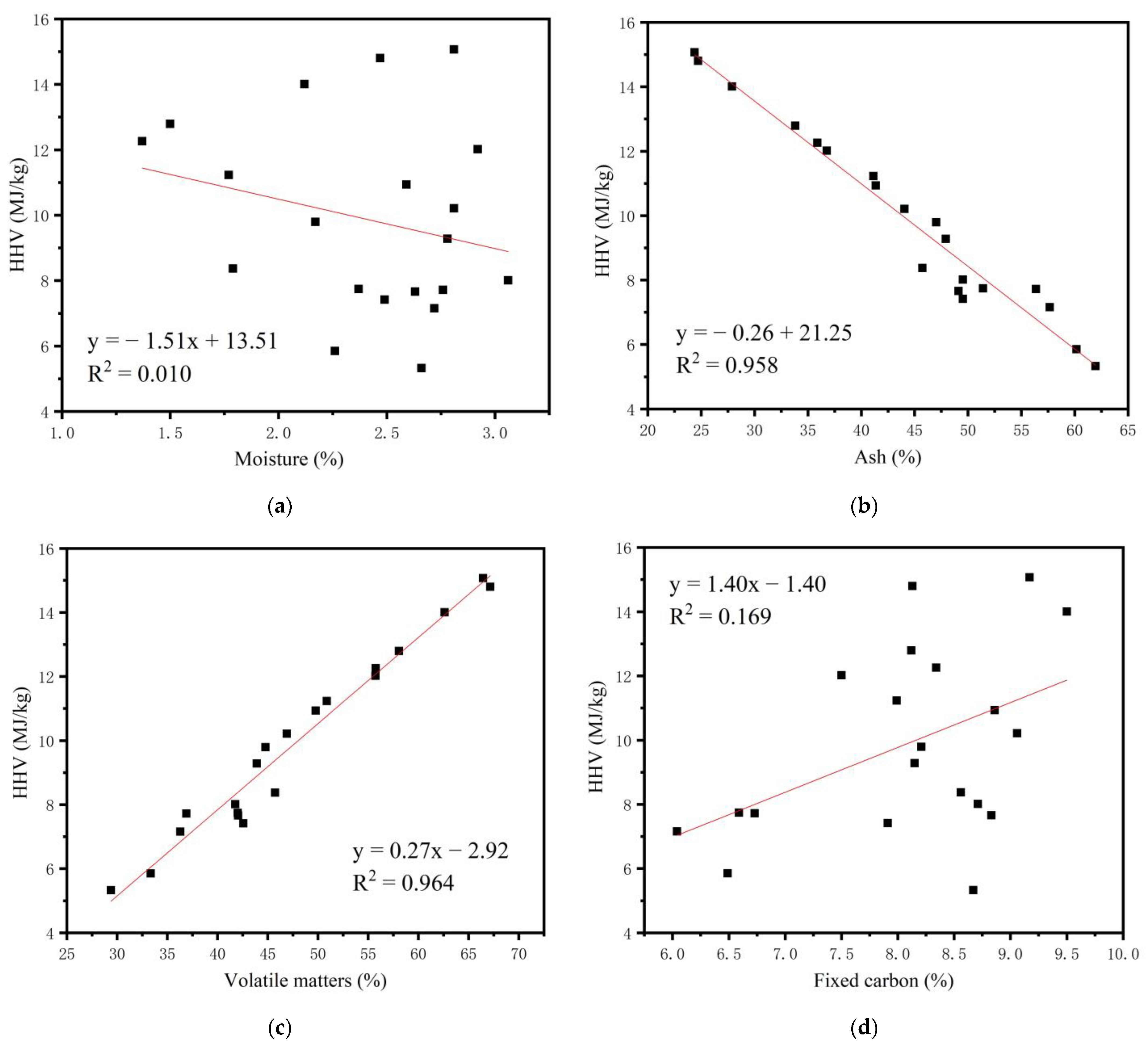
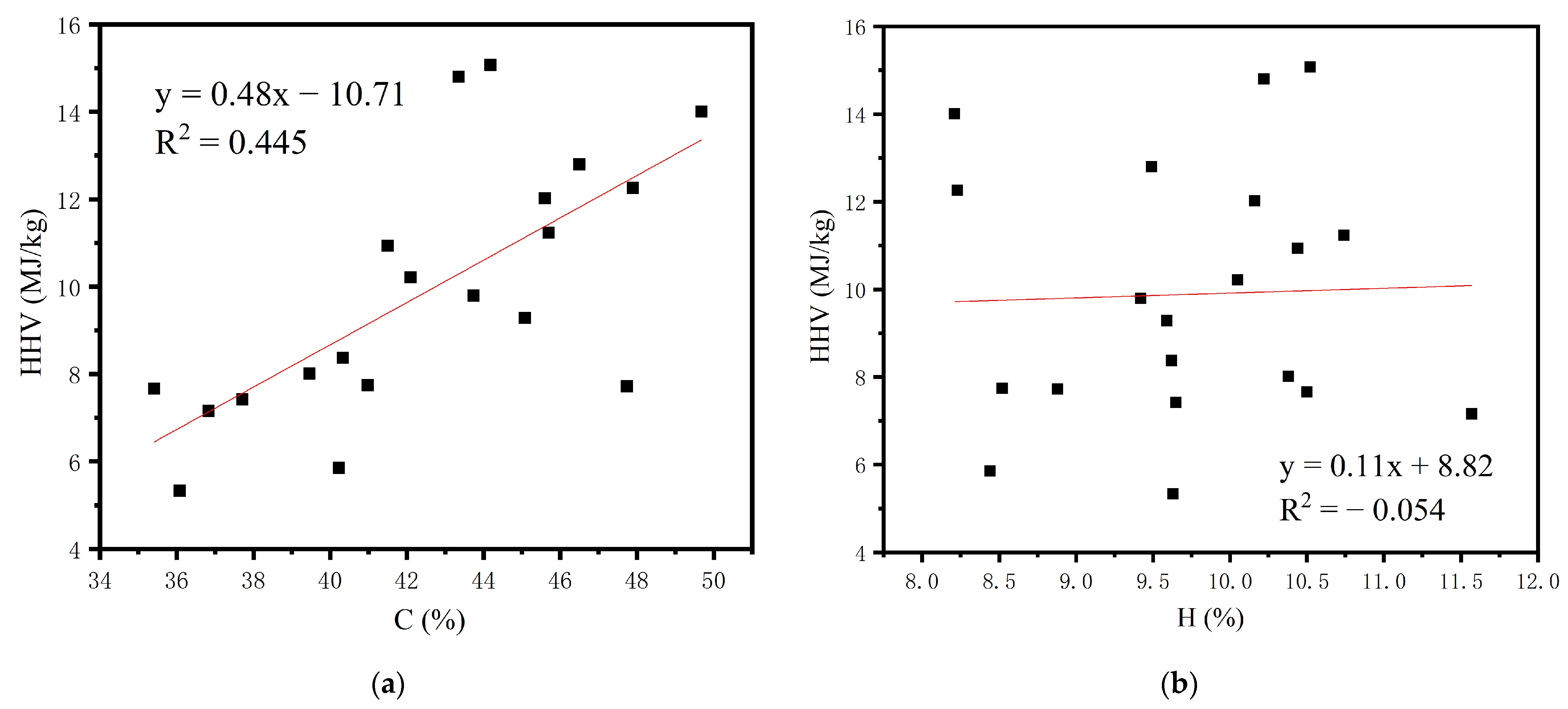
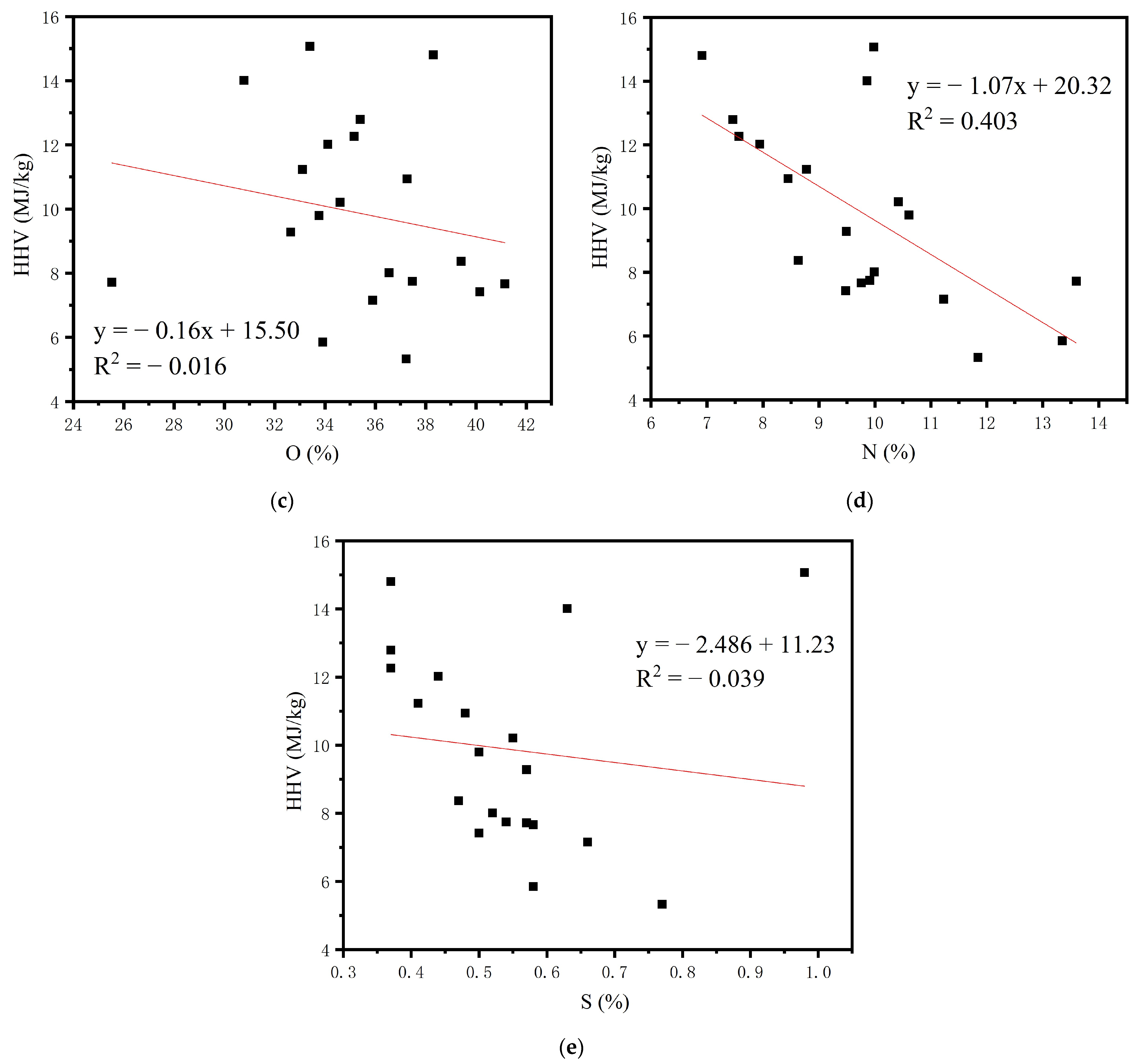
The correlation between the HHV of the sewage sludge samples and their proximate and ultimate analyses data are shown in Figure 2 and Figure 3. For the proximate analysis, the samples with higher VM content and lower ash content had larger HHV (Figure 2b,c) and this result was the same as that of Puchong Thipkhunthod et al. [27]. This indicates that VM was the main factor affecting the HHV of sewage sludge, while in Figure 2a,d it can be seen that there was a clear dispersion in the distribution of the data and it can be inferred that there was no linear correlation between M and FC contents and HHV. For the final analysis, the HHV was larger for samples with higher C and H contents (Figure 3a,b) and the correlation between C content and HHV was high; thus, it was clear that C was the main factor affecting the heating value of sewage sludge, while the distribution of data in the analytical figures (Figure 3c–e) of O, N and S content and HHV had significant divergence and it can be seen that there was no linear correlation between them. From the above results, it can be seen that there is a non-linear relationship between the HHV of sewage sludge and its proximate and ultimate analyses. Therefore, it can be inferred that the commonly used linear model cannot accurately predict the HHV of sludge when modeling based on proximate and ultimate analyses and a non-linear model is required.

3.2. Modeling Back Propagation Neural Network Model

The samples were initially classified by the systematic clustering method and 20 samples were divided into three classes. Subsequently, the clustering analysis of the three classes was performed using K-means clustering method [39] and the distance of each sample from the cluster center was obtained when the number of iterations was 10. The results of the calculations are shown in

Table 2. Characteristics of sewage sludge from different wastewater treatment plants.

Sample	Clustering Categories	Distance	Sample	Clustering Categories	Distance
A1	1	4.580	B2	3	3.385
C5	1	6.443	C3	3	4.079
A5	1	7.884	C1	3	4.240
A4	1	8.364	B1	3	4.841
C6	1	8.989	B5	3	5.813
B3	1	9.979	A3	3	6.256
A8	2	2.250	A6	3	6.473
B4	2	5.740	C4	3	7.512
A2	2	8.260	A7	3	8.462
B6	2	11.549	C2	3	10.181

. According to the distance of the samples from the cluster center, A1, A8 and B2 were divided into test groups for testing the prediction accuracy of the model, while the other samples were divided into training groups as the background data required for modeling.

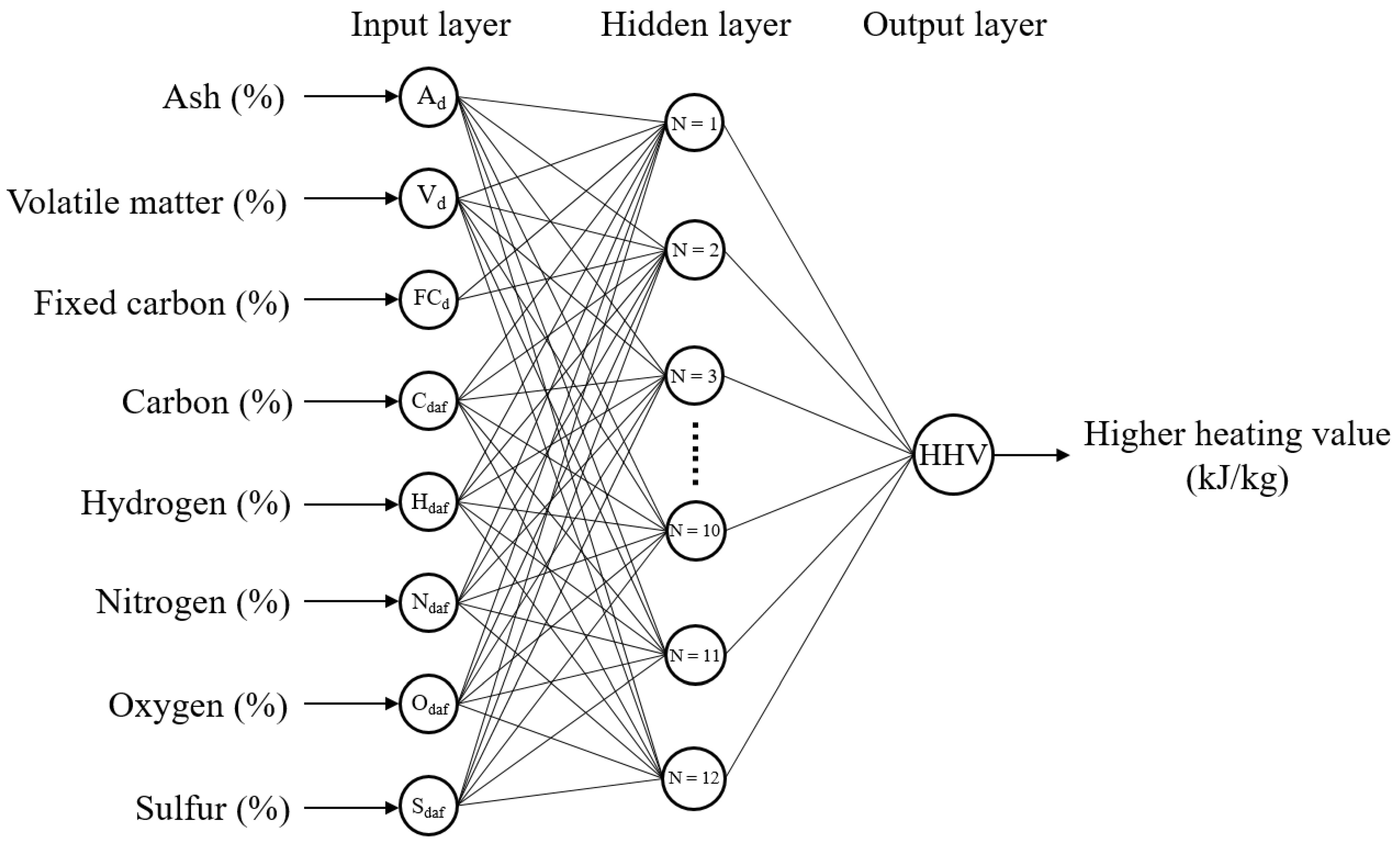
Satyajit Pattanayak et al. [40] and Güleç Fatih et al. [41] investigated three ANN models based on proximate analysis (three inputs), ultimate analysis (five inputs) and proximate-ultimate analysis (eight inputs) for predicting HHV and the results of both studies indicate that the ANN model based on proximate-ultimate analysis had the highest R², which means that the model had the highest accuracy. This may be because the data of the proximate and ultimate analysis represent the characteristics of sewage sludge, thus combining the data of both parts in building the model allows the model to predict HHV in a state that was closer to the nature of sewage sludge itself and therefore, the prediction accuracy of the model was the highest. In this study, the proximate and ultimate analyses data of sewage sludge were used as input parameters. Kolmogorov’s theorem has theoretically proved that a three-layer neural network can approximate any continuous function with arbitrary accuracy, thus a three-layer network structure was chosen for this study. A simple diagram for the model structure established in this study is shown in Figure 4.

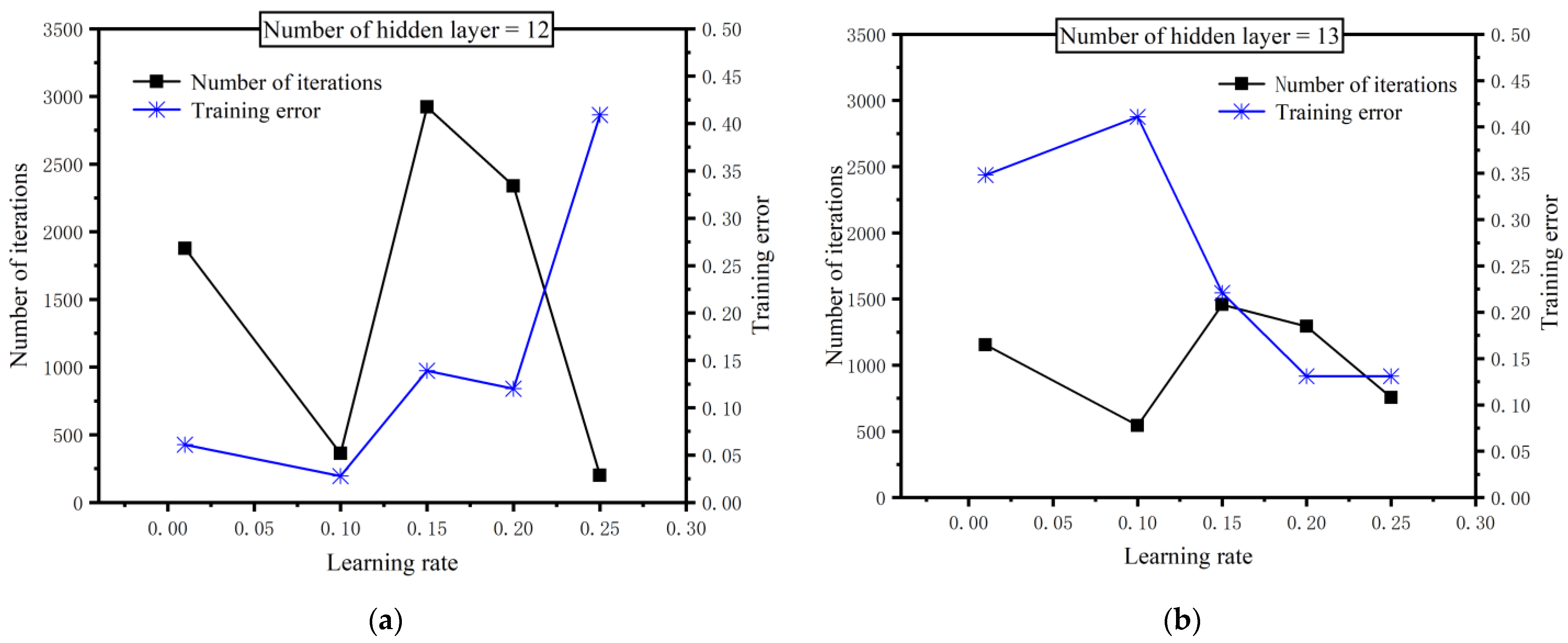
Determining the number of hidden layers was an important factor in building the ANN model. Insufficient hidden layers will make the neural network unable to learn. On the other hand, increasing the number of hidden layers can reduce systematic error, but it will undoubtedly increase the computation time or lead to over-learning and make the neural network lose generalization ability, resulting in the model “over-fitting” [42,43]. Combining Kolmogomv’s theorem, which proposes that the hidden layer should take 2n + 1 (n is the number of input layers) and the empirical formula $N_h=\sqrt{N_i+N_o}+r$, the test range of the hidden layers was 4~17. The stepwise construction method to compare the number of iterations and training errors of the network between different hidden layers at the same learning rate was used and the results are shown in Figure 5. It can be seen that when the number of hidden layers was taken as 12 or 13, the number of iterations and the training errors of the network were at a better level for different learning rates. Therefore, the performance of the model network with 12 or 13 hidden layers at different learning rates was compared, and the results are shown in Figure 6. The best performance of the network could be seen in the table when the hidden layer number was 12 and the learning rate was 0.1, where the number of iterations was 362 and the training error was 0.028.

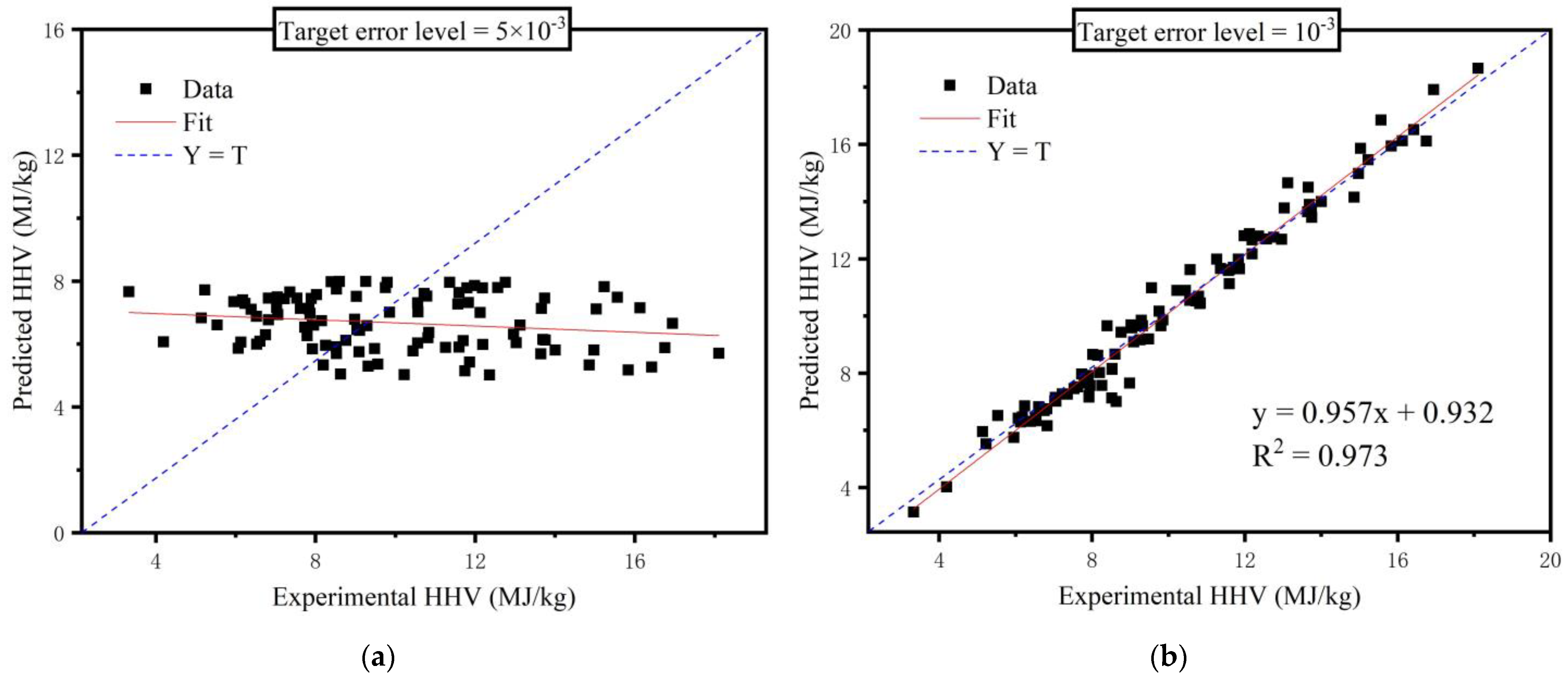
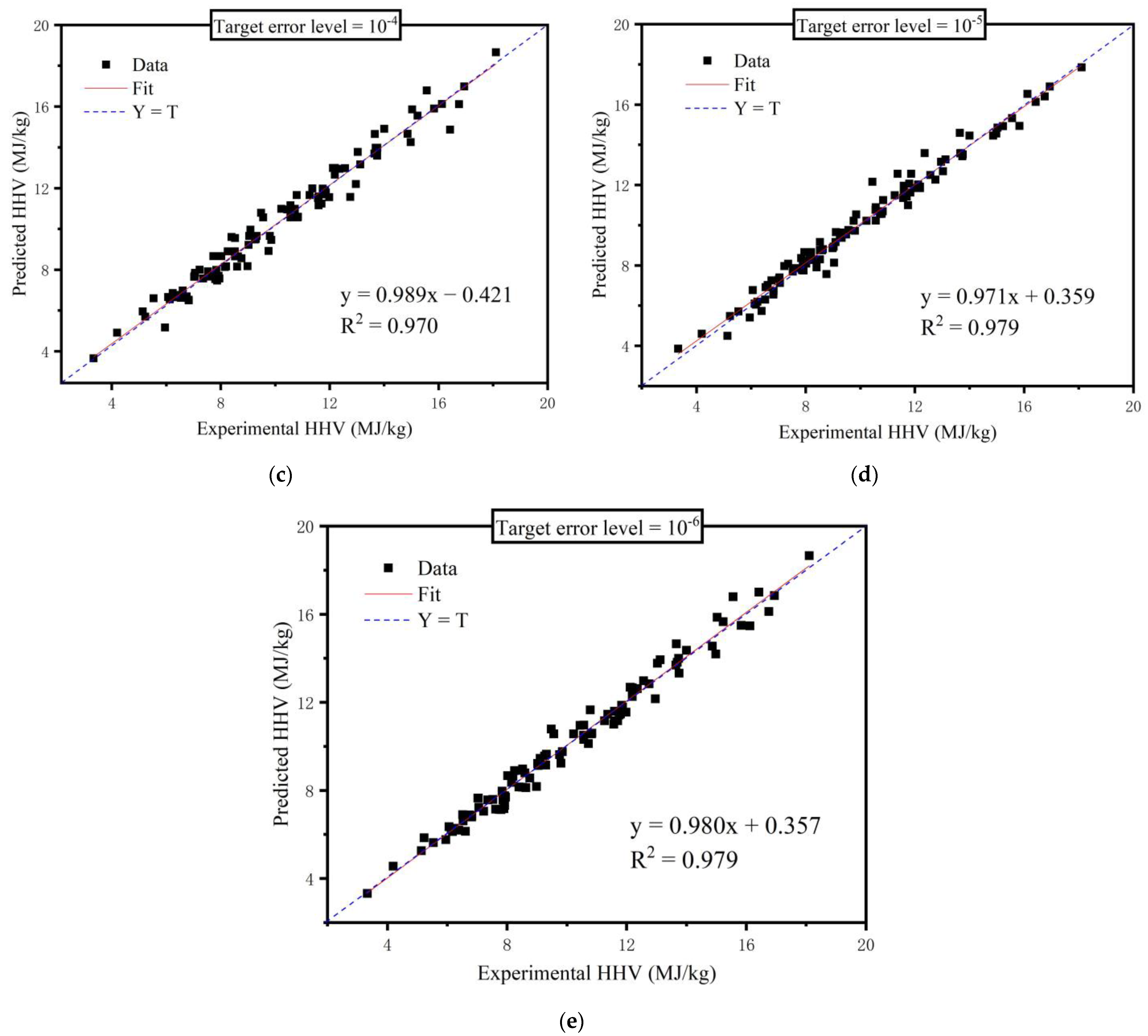
The target error level determines the performance of the model. The larger the error setting, the faster the model achieves the result, but the accuracy is reduced. On the contrary, the smaller the error setting, the more accurate the model will be, but the running time will increase and the error tolerance will decrease. In this study, five target error levels of 5 × 10⁻³, 10⁻³, 10⁻⁴, 10⁻⁵ and 10⁻⁶ were selected for comparison, as shown in Figure 7. It could be seen that the R² was the same for the target error level of 10⁻⁵ and 10⁻⁶, but the latter was more computationally intensive; therefore, the optimal target error level was considered to be 10⁻⁵.

4. Discussion

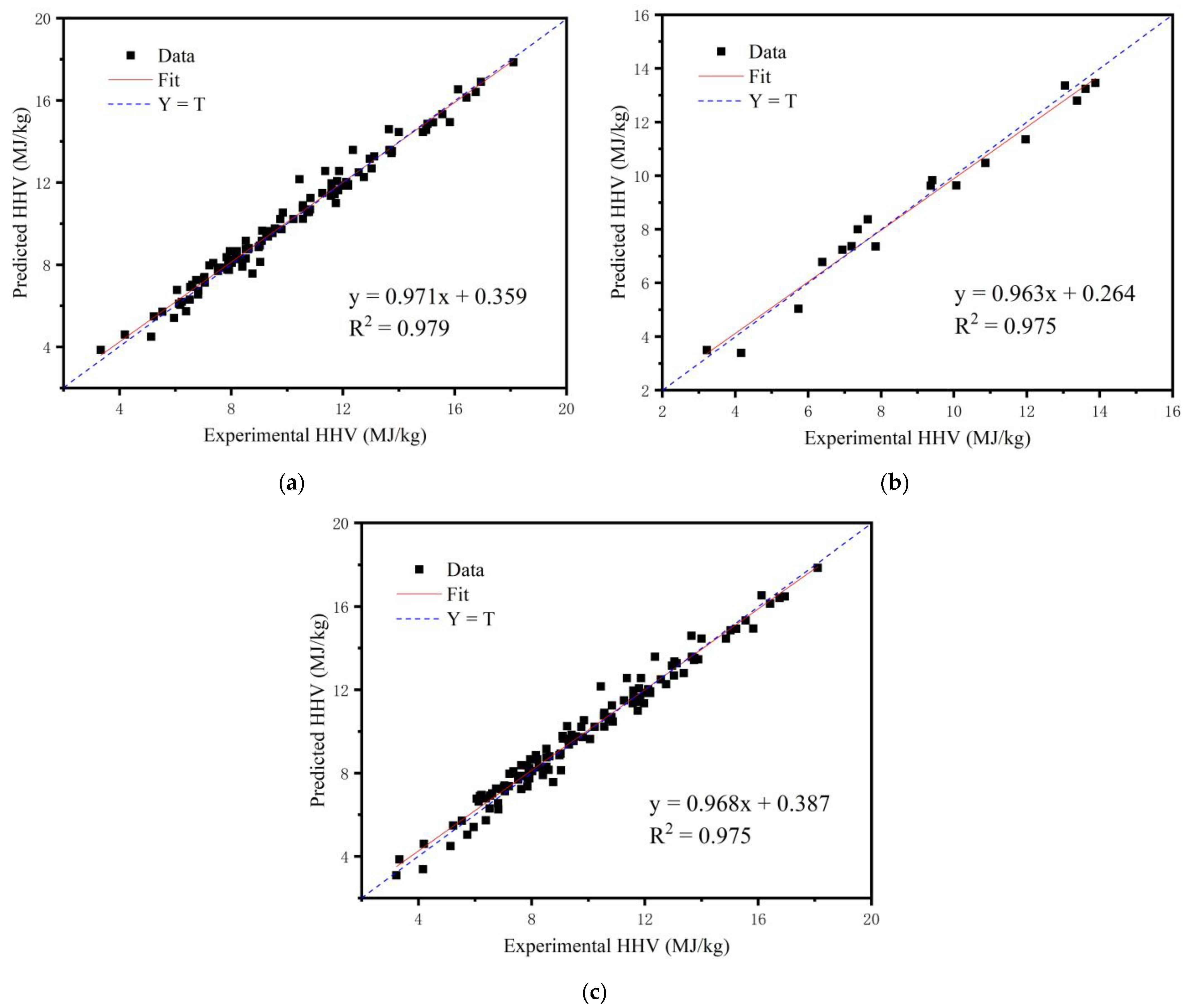
The BPNN model was developed by applying MATLAB software and the input parameters were determined as eight (C, H, O, N, S and VM, FC, Ash) and the output parameter was one: the HHV of the sewage sludge. In order to understand the accuracy of the BPNN model prediction, when comparing the experimental results with the predicted results of the model, the data show a good fit as shown in Figure 8, which demonstrates the goodness of training and testing.

The accuracy of the BPNN model can be understood more intuitively through statistical analysis. In this study, five statistical indexes were selected for analysis and the results were shown in

Table 3. The statistical analysis results of using different sizes of data.

Different Sizes of Data	MSE	RMSE	MAD	MAPE	R2
Train	0.161	0.401	0.319	3.260	0.979
Test	0.209	0.457	0.375	4.651	0.975
All	0.198	0.444	0.385	4.081	0.975

. It can be seen that the R² of the BPNN model in both the training (0.979) and test (0.975) groups were quite high and the corresponding values of MSE (0.161), RMSE (0.401), MAD (0.319) and MAPM (3.260) were small, which indicated that the BPNN model had a high accuracy. Furthermore, it can be observed that the differences between the training and test groups for each of the indexes were small, which reflected the high reliability of the BPNN model. Gülce Çakman et al. [33] constructed an ANN model based on the Levenberg–Marquardt algorithm to predict the HHV of biochar, with R² of 0.99 for both the training and test groups. Amir Dashti et al. [42] built four different ANN models, where the ANFIS model with a BP algorithm had an R² of 0.97 for both training and test groups, which was similar to the current study. This indicates that the BPNN model had a high accuracy and can be used to predict the HHV of sewage sludge.

In order to better validate the accuracy of the BPNN model, several linear empirical equations were summarized from the previous literature for predicting the HHV of sewage sludge, as shown in

Table 4. Various HHV prediction models from the literature.

Input Parameters	Equation	Reference
Proximate analysis (FC, VM, Ash)	HHV = 353.6FC + 155.9VM − 7.8Ash	Jigisha Parikh et al. [44]
	HHV = 255.75VM + 283.88FC − 2386.38	Puchong Thipkhunthod et al. [27]
Ultimate analysis (C, H, O, N, S)	HHV = 430.2C − 186.7H−127.4N + 178.6S + 184.2O − 2379.9	Puchong Thipkhunthod et al. [27]
	HHV = 349.1C + 1178.3H + 100.5S − 103.4O − 15.1N − 21.1Ash	S. A. Channiwala et al. [45]

. Two of the equations derived from the study by Puchong Thipkhunthod et al. [27], which were considered to be the most suitable for predicting the HHV of sewage sludge.

Table 5. Comparison of the models for predicting of HHV using all data.

Models	MSE	RMSE	MAD	MAPE	R2
Jigisha Parikh et al. [44]	2.262	1.504	1.188	15.546	0.722
Puchong Thipkhunthod et al. [27]	5.161	2.272	2.198	24.574	0.365
Puchong Thipkhunthod et al. [27]	1.588	1.178	1.104	11.862	0.797
S. A. Channiwala et al. [45]	2.591	1.610	1.531	15.743	0.688
The BPNN model in this study	0.198	0.444	0.385	4.081	0.975

shows the results obtained from the statistical analysis of all models. From the table, it can be seen that the BPNN model had the highest R² (0.975). The reason for the superiority of the BPNN model over the other models may be that most of the models were modeled only based on the proximate or ultimate analysis, which would exclude some of the factors related to HHV and thus lead to poor prediction accuracy. Additionally, there was an irrelevance between the proximate and ultimate analysis of sewage sludge and its HHV and the linear model was not usable as the best option for predicting the HHV of sewage sludge. After checking other statistical results (MSE, RMSE, MAD and MAPE), it was further shown that the accuracy of the BPNN model was higher than other models. This was because the BPNN model had the lowest index for all the indicators (MSE = 0.198, RMSE = 0.444, MAD = 0.385 and MAPE = 4.081). This study clearly shows that the developed BPNN model was most suitable for predicting the HHV of sewage sludge.

5. Conclusions

In this study, the HHV predicted by the BPNN model was very close to the measured HHV. The percentage of relative error within 5% was 76.5% and the percentage of absolute error within 10% was 100%. The accuracy of the model was further illustrated by the calculated results of statistical analysis, where the R² of MSE, RMSE, MAD and MAPE were 0.209, 0.457, 0.375, 4.651 and 0.975, respectively. Several previously proposed empirical models were selected for comparison with the BPNN model. The results show that the BPNN model predicts an HHV (MAD = 0.385, MAPE = 4.081 and R² = 0.975) more accurately than the other models. The results of this study show that the non-linear model built by an artificial neural network can replace the oxygen bomb calorimeter to measure the HHV of sewage sludge and provide a more convenient option for subsequent methods of recovering energy from sewage sludge (pyrolysis, anaerobic digestion, etc.). In the future, we will expand the database by collecting different types of sewage sludge and explore the performance of other ANN models in predicting sewage sludge HHV to find the most suitable model.

References

- Wei, L.; Xia, X.; Zhu, F.; Li, Q.; Xue, M.; Li, J.; Sun, B.; Jiang, J.; Zhao, Q. Dewatering efficiency of sewage sludge during Fe(2+)-activated persulfate oxidation: Effect of hydrophobic/hydrophilic properties of sludge EPS. Water Res. 2020, 181, 115903. [Google Scholar] [CrossRef] [PubMed]
- Bai, B.; Rao, D.; Chang, T.; Guo, Z. A nonlinear attachment-detachment model with adsorption hysteresis for suspension-colloidal transport in porous media. J. Hydrol. 2019, 578, 124080. [Google Scholar] [CrossRef]
- Bai, B.; Wang, Y.; Rao, D.; Bai, F. The Effective Thermal Conductivity of Unsaturated Porous Media Deduced by Pore-Scale SPH Simulation. Front. Earth Sci. 2022, 10, 943853. [Google Scholar] [CrossRef]
- Hoang, S.A.; Bolan, N.; Madhubashani, A.M.P.; Vithanage, M.; Perera, V.; Wijesekara, H.; Wang, H.; Srivastava, P.; Kirkham, M.B.; Mickan, B.S.; et al. Treatment processes to eliminate potential environmental hazards and restore agronomic value of sewage sludge: A review. Environ. Pollut. 2022, 293, 118564. [Google Scholar] [CrossRef] [PubMed]
- Ge, D.; Yuan, H.; Xiao, J.; Zhu, N. Insight into the enhanced sludge dewaterability by tannic acid conditioning and pH regulation. Sci. Total Environ. 2019, 679, 298–306. [Google Scholar] [CrossRef]
- Wang, C.; Fan, Y.; Hornung, U.; Zhu, W.; Dahmen, N. Char and tar formation during hydrothermal treatment of sewage sludge in subcritical and supercritical water: Effect of organic matter composition and experiments with model compounds. J. Clean. Prod. 2020, 242, 118586. [Google Scholar] [CrossRef]
- Fang, X.; Wang, Q.; Wang, J.; Xiang, Y.; Wu, Y.; Zhang, Y. Employing extreme value theory to establish nutrient criteria in bay waters: A case study of Xiangshan Bay. J. Hydrol. 2021, 603, 127146. [Google Scholar] [CrossRef]
- Li, T.; Su, T.; Wang, J.; Zhu, S.; Zhang, Y.; Geng, Z.; Wang, X.; Gao, Y. Simultaneous removal of sulfate and nitrate from real high-salt flue gas wastewater concentrate via a waste heat crystallization route. J. Clean. Prod. 2023, 382, 135262. [Google Scholar] [CrossRef]
- Gaur, R.Z.; Khoury, O.; Zohar, M.; Poverenov, E.; Darzi, R.; Laor, Y.; Posmanik, R. Hydrothermal carbonization of sewage sludge coupled with anaerobic digestion: Integrated approach for sludge management and energy recycling. Energy Convers. Manag. 2020, 224, 113353. [Google Scholar] [CrossRef]
- Oliveira, A.S.; Sarrion, A.; Baeza, J.A.; Diaz, E.; Calvo, L.; Mohedano, A.F.; Gilarranz, M.A. Integration of hydrothermal carbonization and aqueous phase reforming for energy recovery from sewage sludge. Chem. Eng. J. 2022, 442, 136301. [Google Scholar] [CrossRef]
- Liu, W.; Zheng, J.; Ou, X.; Liu, X.; Song, Y.; Tian, C.; Rong, W.; Shi, Z.; Dang, Z.; Lin, Z. Effective Extraction of Cr(VI) from Hazardous Gypsum Sludge via Controlling the Phase Transformation and Chromium Species. Environ. Sci. Technol. 2018, 52, 13336–13342. [Google Scholar] [CrossRef] [PubMed]
- Wang, Z.; Liu, X.; Ni, S.-Q.; Zhuang, X.; Lee, T. Nano zero-valent iron improves anammox activity by promoting the activity of quorum sensing system. Water Res. 2021, 202, 117491. [Google Scholar] [CrossRef] [PubMed]
- Xu, D.; Li, J.; Liu, J.; Qu, X.; Ma, H. Advances in continuous flow aerobic granular sludge: A review. Process Saf. Environ. Prot. 2022, 163, 27–35. [Google Scholar] [CrossRef]
- Xu, Y.; Dai, X. Integrating multi-state and multi-phase treatment for anaerobic sludge digestion to enhance recovery of bio-energy. Sci. Total Environ. 2020, 698, 134196. [Google Scholar] [CrossRef] [PubMed]
- Passos, J.; Alves, O.; Brito, P. Management of municipal and construction and demolition wastes in Portugal: Future perspectives through gasification for energetic valorisation. Int. J. Environ. Sci. Technol. 2020, 17, 2907–2926. [Google Scholar] [CrossRef]
- Chen, L.; Liao, Y.; Ma, X. Economic analysis on sewage sludge drying and its co-combustion in municipal solid waste power plant. Waste Manag. 2021, 121, 11–22. [Google Scholar] [CrossRef]
- Zhao, Y.; Li, Q.; Cui, Q.; Ni, S.-Q. Nitrogen recovery through fermentative dissimilatory nitrate reduction to ammonium (DNRA): Carbon source comparison and metabolic pathway. Chem. Eng. J. 2022, 441, 135938. [Google Scholar] [CrossRef]
- Mosko, J.; Pohorely, M.; Skoblia, S.; Beno, Z.; Jeremias, M. Detailed Analysis of Sewage Sludge Pyrolysis Gas: Effect of Pyrolysis Temperature. Energies 2020, 13, 4087. [Google Scholar] [CrossRef]
- Zhang, X.; Ma, F.; Yin, S.; Wallace, C.; Soltanian, M.R.; Dai, Z.; Ritzi, R.W.; Ma, Z.; Zhan, C.; Lu, X. Application of upscaling methods for fluid flow and mass transport in multi-scale heterogeneous media: A critical review. Appl. Energy 2021, 303, 117603. [Google Scholar] [CrossRef]
- Zhao, L.; Du, M.; Du, W.; Guo, J.; Liao, Z.; Kang, X.; Liu, Q. Evaluation of the Carbon Sink Capacity of the Proposed Kunlun Mountain National Park. Int. J. Environ. Res. Public Health 2022, 19, 9887. [Google Scholar] [CrossRef]
- Xu, L.; Yuan, J. Online identification of the lower heating value of the coal entering the furnace based on the boiler-side whole process models. Fuel 2015, 161, 68–77. [Google Scholar] [CrossRef]
- Dashti, A.; Noushabadi, A.S.; Asadi, J.; Raji, M.; Chofreh, A.G.; Klemes, J.J.; Mohammadi, A.H. Review of higher heating value of municipal solid waste based on analysis and smart modelling. Renew. Sustain. Energy Rev. 2021, 151, 111591. [Google Scholar] [CrossRef]
- Ghugare, S.B.; Tiwary, S.; Elangovan, V.; Tambe, S.S. Prediction of Higher Heating Value of Solid Biomass Fuels Using Artificial Intelligence Formalisms. Bioenergy Res. 2014, 7, 681–692. [Google Scholar] [CrossRef]
- Cordero, T.; Marquez, F.; Rodriguez-Mirasol, J.; Rodriguez, J.J. Predicting heating values of lignocellulosics and carbonaceous materials from proximate analysis. Fuel 2001, 80, 1567–1571. [Google Scholar] [CrossRef]
- Kathiravale, S.; Yunus, M.N.M.; Sopian, K.; Samsuddin, A.H.; Rahman, R.A. Modeling the heating value of Municipal Solid Waste. Fuel 2003, 82, 1119–1125. [Google Scholar] [CrossRef]
- Choi, H.L.; Sudiarto, S.I.A.; Renggaman, A. Prediction of livestock manure and mixture higher heating value based on fundamental analysis. Fuel 2014, 116, 772–780. [Google Scholar] [CrossRef]
- Thipkhunthod, P.; Meeyoo, V.; Rangsunvigit, P.; Kitiyanan, B.; Siemanond, K.; Rirksomboon, T. Predicting the heating value of sewage sludges in Thailand from proximate and ultimate analyses. Fuel 2005, 84, 849–857. [Google Scholar] [CrossRef]
- Akkaya, E. ANFIS based prediction model for biomass heating value using proximate analysis components. Fuel 2016, 180, 687–693. [Google Scholar] [CrossRef]
- Petkovic, B.; Petkovic, D.; Kuzman, B. Adaptive neuro fuzzy predictive models of agricultural biomass standard entropy and chemical exergy based on principal component analysis. Biomass Convers. Biorefinery 2022, 12, 2835–2845. [Google Scholar] [CrossRef]
- Xing, J.; Luo, K.; Wang, H.; Gao, Z.; Fan, J. A comprehensive study on estimating higher heating value of biomass from proximate and ultimate analysis with machine learning approaches. Energy 2019, 188, 116077. [Google Scholar] [CrossRef]
- Aladejare, A.E.; Onifade, M.; Lawal, A.I. Application of metaheuristic based artificial neural network and multilinear regression for the prediction of higher heating values of fuels. Int. J. Coal Prep. Util. 2022, 42, 1830–1851. [Google Scholar] [CrossRef]
- Kapetanakis, T.N.; Vardiambasis, I.O.; Nikolopoulos, C.D.; Konstantaras, A.I.; Trang, T.K.; Khuong, D.A.; Tsubota, T.; Keyikoglu, R.; Khataee, A.; Kalderis, D. Towards Engineered Hydrochars: Application of Artificial Neural Networks in the Hydrothermal Carbonization of Sewage Sludge. Energies 2021, 14, 3000. [Google Scholar] [CrossRef]
- Cakman, G.; Gheni, S.; Ceylan, S. Prediction of higher heating value of biochars using proximate analysis by artificial neural network. Biomass Convers. Biorefinery 2021, 1–9. [Google Scholar] [CrossRef]
- Taki, M.; Rohani, A. Machine learning models for prediction the Higher Heating Value (HHV) of Municipal Solid Waste (MSW) for waste-to-energy evaluation. Case Stud. Therm. Eng. 2022, 31, 101823. [Google Scholar] [CrossRef]
- Genuino, D.A.D.; Bataller, B.G.; Capareda, S.C.; de Luna, M.D.G. Application of artificial neural network in the modeling and optimization of humic acid extraction from municipal solid waste biochar. J. Environ. Chem. Eng. 2017, 5, 4101–4107. [Google Scholar] [CrossRef]
- Akkaya, A.V. Predicting Coal Heating Values Using Proximate Analysis via a Neural Network Approach. Energy Sources Part A-Recovery Util. Environ. Eff. 2013, 35, 253–260. [Google Scholar] [CrossRef]
- Chang, Y.F.; Lin, C.J.; Chyan, J.M.; Chen, I.M.; Chang, J.E. Multiple regression models for the lower heating value of municipal solid waste in Taiwan. J. Environ. Manag. 2007, 85, 891–899. [Google Scholar] [CrossRef]
- Chan, W.P.; Wang, J.-Y. Comprehensive characterisation of sewage sludge for thermochemical conversion processes—Based on Singapore survey. Waste Manag. 2016, 54, 131–142. [Google Scholar] [CrossRef]
- Kanungo, T.; Mount, D.M.; Netanyahu, N.S.; Piatko, C.D.; Silverman, R.; Wu, A.Y. An efficient k-means clustering algorithm: Analysis and implementation. IEEE Trans. Pattern Anal. Mach. Intell. 2002, 24, 881–892. [Google Scholar] [CrossRef]
- Pattanayak, S.; Loha, C.; Hauchhum, L.; Sailo, L. Application of MLP-ANN models for estimating the higher heating value of bamboo biomass. Biomass Convers. Biorefinery 2021, 11, 2499–2508. [Google Scholar] [CrossRef]
- Gulec, F.; Pekaslan, D.; Williams, O.; Lester, E. Predictability of higher heating value of biomass feedstocks via proximate and ultimate analyses-A comprehensive study of artificial neural network applications. Fuel 2022, 320, 123944. [Google Scholar] [CrossRef]
- Dashti, A.; Noushabadi, A.S.; Raji, M.; Razmi, A.; Ceylan, S.; Mohammadi, A.H. Estimation of biomass higher heating value (HHV) based on the proximate analysis: Smart modeling and correlation. Fuel 2019, 257, 115931. [Google Scholar] [CrossRef]
- Lee, K.M.; Zanil, M.F.; Chan, K.K.; Chin, Z.P.; Liu, Y.C.; Lim, S. Synergistic ultrasound-assisted organosolv pretreatment of oil palm empty fruit bunches for enhanced enzymatic saccharification: An optimization study using artificial neural networks. Biomass Bioenergy 2020, 139, 105621. [Google Scholar] [CrossRef]
- Parikh, J.; Channiwala, S.A.; Ghosal, G.K. A correlation for calculating HHV from proximate analysis of solid fuels. Fuel 2005, 84, 487–494. [Google Scholar] [CrossRef]
- Channiwala, S.A.; Parikh, P.P. A unified correlation for estimating HHV of solid, liquid and gaseous fuels. Fuel 2002, 81, 1051–1063. [Google Scholar] [CrossRef]
Figure 1.
Distribution of different wastewater treatment plants.
Figure 2.
Correlation between HHV and proximate analysis data: (a) indicates the correlation between moisture and HHV; (b) indicates the correlation between ash and HHV; (c) indicates the correlation between VM and HHV; (d) indicates the correlation between FC and HHV.
Figure 3.
Correlation between HHV and ultimate analysis data: (a) indicates the correlation between carbon and HHV; (b) indicates the correlation between hydrogen and HHV; (c) indicates the correlation between oxygen and HHV; (d) indicates the correlation between nitrogen and HHV; (e) indicates the correlation between sulfur and HHV.
Figure 4.
The architecture of the three-layered ANN model.
Figure 5.
Performance comparison with different hidden layers: (a) indicates the situation where the learning rate is 0.01; (b) indicates the situation where the learning rate is 0.10; (c) indicates the situation where the learning rate is 0.15; (d) indicates the situation where the learning rate is 0.20.
Figure 6.
Performance of the network with different hidden layers: (a) indicates the situation where the hidden layers are 12; (b) indicates the situation where the hidden layers are 13.
Figure 7.
Network simulation results with different target error level: (a) indicates the situation where the target error level is 5 × 10⁻³; (b) indicates the situation where the target error level is 10−3; (c) indicates the situation where the target error level is 10−4; (d) indicates the situation where the target error level is 10−5; (e) indicates the situation where the target error level is 10−6.
Figure 8.
Comparison of predicted HHV and experimental HHV: (a) training group data; (b) testing group data; (c) all data.