Article

Analysis of Long-Term Trend of Stream Flow and Interaction Effect of Land Use and Land Cover on Water Yield by SWAT Model and Statistical Learning in Part of Urmia Lake Basin, Northwest of Iran

by
Mohamad Sakizadeh
1,*,
Adam Milewski
2,* and
Mohammad Taghi Sattari
3,4
1
Department of Environmental Sciences, Shahid Rajaee Teacher Training University, Shahid Shabanlou Avenue, Lavizan, Tehran 16785-163, Iran
2
Department of Geology, University of Georgia, 210 Field Street, Athens, GA 30602, USA
3
Department of Water Engineering, Agriculture Faculty, University of Tabriz, Tabriz 51666-16471, Iran
4
Department of Agricultural Engineering, Faculty of Agriculture, Ankara University, Ankara 06100, Turkey
*
Authors to whom correspondence should be addressed.
Water 2023, 15(4), 690; https://doi.org/10.3390/w15040690
Submission received: 27 December 2022 / Revised: 30 January 2023 / Accepted: 3 February 2023 / Published: 9 February 2023
(This article belongs to the Section Hydrogeology)

Abstract

:
The water yield produced at the outlet of a sub-basin is the combination of multiple interacting land uses. In the majority of previous research, while accounting for the effect of land use and land cover (LULC) on water yield, the hydrologic components of a watershed have been attributed to the dominant land use class within that sub-basin. We adopted an approach to investigate the interaction effect of LULC on water yield (WYLD) using the Johnson–Neyman (JN) method. The soil and water assessment tool (SWAT) model was employed in the Urmia Lake Basin (ULB) to estimate the WYLD following successful calibration and validation of the model by stream flow. It was found that in each sub-basin, the effect of the soil class on the WYLD was statistically significant only when the area of rangeland was less than 717 ha and when the area of agricultural lands was less than 633 ha. On the other hand, the trend of stream flow was assessed over 70 years at two stations in the Urmia Lake Basin (ULB) using the Bayesian Estimator of Abrupt change, Seasonal change, and Trend (BEAST). The year 1991 turned out to be the most likely change point in both stations. A significant decrease in Urmia Lake’s water level started in 1995, which indicated that part of this shrinkage was most likely caused by water inflow reduction over a 4-year time delay. Besides identifying the most probable seasonal and trend change points, this method has the additional capability to analyze the uncertainty of estimated points, which was lacking in earlier methods.

1. Introduction

Urmia Lake, located in the northwest of Iran, is the second largest saline lake in the world that plays a significant role in sustainable ecosystem services in this part of the country. However, as a result of natural and human-induced factors, the lake water level has significantly decreased over the last two decades and is most recently on the verge of complete desiccation. Accordingly, analysis of the long-term trend of stream flow in rivers located in the Urmia Lake Basin (ULB) can shed light on the magnitude and intensity of inflow reduction as a likely cause of the Urmia Lake drying process. In this respect, the most common non-parametric trend analysis technique is the Mann–Kendall test [1,2] which is a distribution-free approach that is robust against outliers [3], while the most traditional approach for detecting abrupt changes is the Pettitt test [4]. Nonetheless, the main shortcomings of the latest approaches are their inability to quantify trends and changes, along with their limited efficiency to identify non-linear and abrupt changes. These disadvantages necessitate the development of more advanced approaches to detect abrupt change, seasonal change, and trends simultaneously, while also accounting for non-linear trends in time series. To address this problem, in this current research, a novel Bayesian model averaging, known as the Bayesian Estimator of Abrupt change, Seasonal change, and Trend (BEAST), which was first developed by Zhao et al. [5], was utilized in order to not only quantify the trend and abrupt changes in a time series of river flow in two hydrometric stations located in the ULB, but also to take into account the uncertainty in trend estimation. This research is the first application of this approach for the trend analysis of stream flow. This technique proved its efficiency for analyzing the long-term trend and abrupt changes in river water quality in a recent study [6].
On the other hand, the benefits that humans derive from nature are called ecosystem services (ES), which covers a broad-spectrum including provisioning, regulating, supporting, and cultural services. One of the most important aspects of hydrologic provision ecosystem services is water yield (WYLD), due to its effect on the maintenance of natural irrigation and drainage, the buffering of extremes in the discharge of rivers, etc. [7]. The dryland and semi-dryland ecosystems represent one of the most vulnerable environments for maintaining viable ES because of the imbalance between water supply and demand [8]. This condition is dominant in the northwest of Iran; thus, the quantification of hydrologic provision ecosystem services (water yield) and the identification of its interaction with external driving forces, including climate variables and land use, is of paramount importance for the management of water resources in the respective area of study. Regarding the effect of land use and land cover (LULC) on hydrological components of the watershed, including WYLD, there are many tools to establish the interaction between land use changes and local hydrology. These include spatially dispersed hydrological models, such as Integrated Valuation of Ecosystem Services and Tradeoffs (InVEST) and the Soil and Water Assessment Tool (SWAT), together with artificial intelligence models like Artificial Intelligence for Ecosystem Services (ARIES); however, spatially explicit hydrologic models are the most reliable tools. For instance, Anand et al. [9] investigated the change in LULC in the Ganges River Basin in India through a land change modeler in the base-time and future time period followed by the effect of these land use modifications on the hydrological regimes of the watershed using the SWAT model. It was concluded that urbanization was the most important contributor to the increase in WYLD and surface runoff. Similar research was also conducted in Iran within the area of this study. In particular, Balist et al. [10] investigated the effect of land use and climate parameters on water yield using the InVEST model in the Sirvan River Basin located in two western provinces of Iran. Roushangar et al. [11] studied the impacts of LULC changes on the water requirement of the Urmia Lake Basin using Cellular Automata-Markov (CA-Marko) and NETWAT models. Finally, Zaman et al. [12] evaluated the effect of climate adaptation strategies on agricultural production in the Siminehrud Watershed and its effect on inflow into Lake Urmia using the SWAT model. Nevertheless, there has not been any previous research regarding the effect of LULC changes on hydrological components using the SWAT model in the Urmia Lake Basin to the best of the authors’ knowledge. Meanwhile, it should be noted that the water yield produced at the outlet of a sub-basin is due to multiple interacting land uses. In the majority of previous research, while accounting for the effect of LULC on water yield, the hydrologic components of a watershed have been attributed to the dominant land use class within that sub-basin [13,14,15]. However, this may not be an accurate approach. Analysis of the interaction and effect of LULC on WYLD will help to better plan for the conservation of vulnerable sub-watersheds in terms of water resource management.
In this respect, the most common method for interaction analysis in environmental sciences uses simple slopes in which the researcher seeks the conditional slope of the focal predictor associated with some particular values of the moderator (e.g., a third variable influencing the magnitude of the linear relationship between the explanatory variable and the response variable). That is to say, what would be the slope of regression when the moderator is held at zero? For this purpose, the conditional effect (simple slopes) of the focal predictor at specified values of the moderator is analyzed. However, the problem with this approach is that only small values of moderating variables are arbitrarily selected (e.g., the mean as well as the mean plus/minus one standard deviation) in order to find the slope of the focal predictor. The arbitrarily selected values may even reside outside the range of observed values for some skewed data (e.g., when the mean plus/minus one standard deviation is adopted). Nevertheless, the researchers may primarily be interested in examining the conditional effect of the focal predictor across the entire range of the moderator.
In this study, to analyze the interaction effect of land use and land cover at the sub-basin scale, we applied a statistical learning technique known as, the Johnson–Neyman (JN) method [16] to (1) assess the conditional effect of the focal predictor (a LULC within the area of the respective sub-basin) over the entire range of the moderating variable (another LULC within the area of the respective sub-basin that interacts with the focal predictor); to (2) determine the regions of significance and non-significance for a linear relationship between the focal predictor and the response (water yield in this case) associated with the moderator; and to (3) estimate the confidence bands of predictions. The JN method was employed following the calibration and validation of streamflow to estimate the amount of WYLD at the sub-basin scale. This study was the first application of statistical learning to investigate the interaction effect of the LULC on water yield within environmental and water resources research. In this respect, by statistical learning, we mean identifying the structure of input data based on its statistical properties [17], which comprise a wide range of methods that are applicable in different fields of study, including machine learning techniques.
Consequently, the objectives of the current research were to (i) investigate the association between the long-term trend of stream flow and Urmia Lake desiccation using a novel Bayesian approach known as BEAST and to (ii) estimate the interaction effects of LULC on water yield at the sub-basin scale using the JN method.

2. Materials and Methods
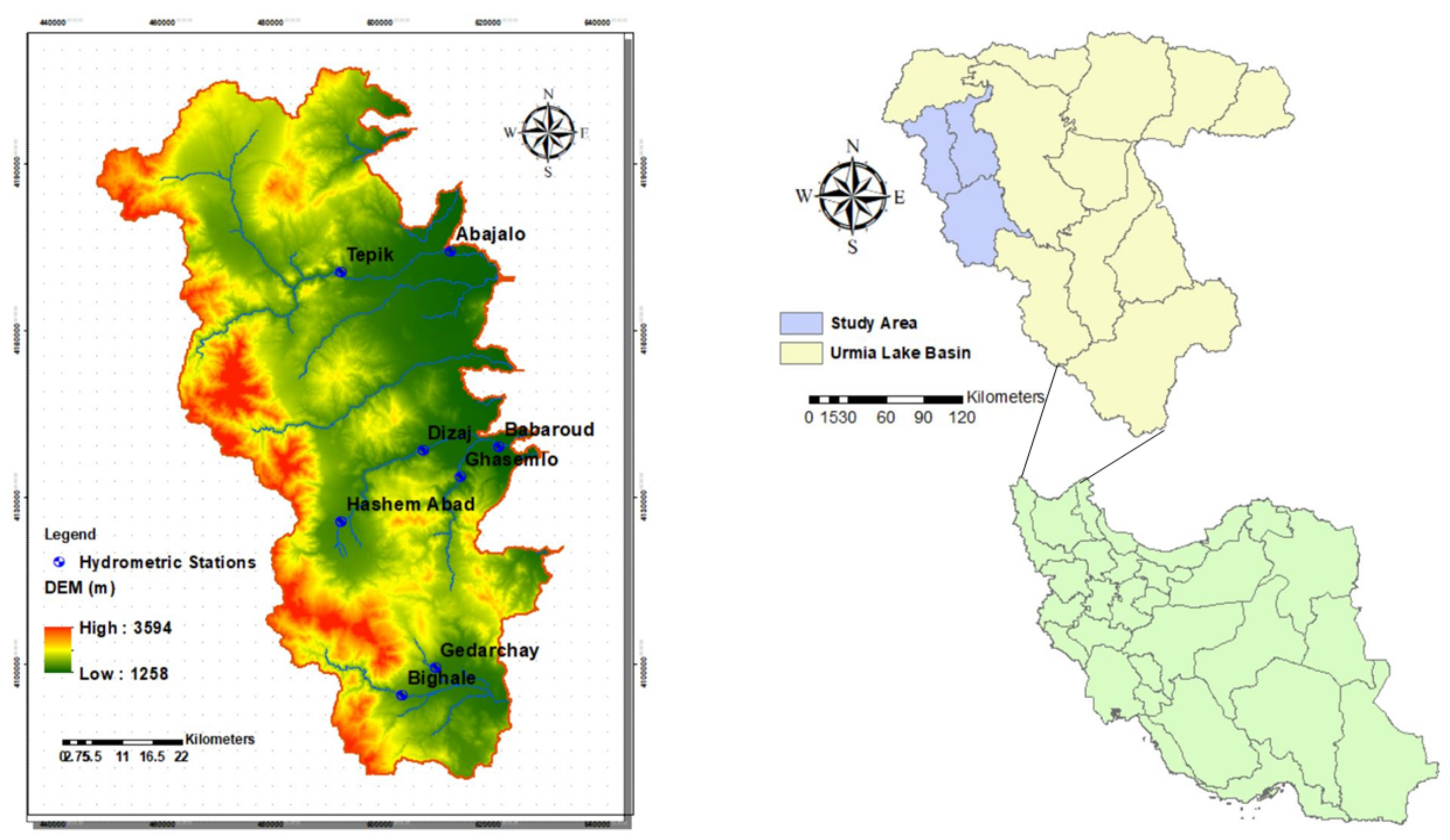
2.1. Study Area

The study region is part of the West Azerbaijan Province that is located in the northwest of Iran and has an area of about 5700 km2 (Figure 1). In particular, it covers the western part of Urmia Lake, the largest lake in Iran, which is on the threshold of complete desiccation due to decreases in its water level originating from a combination of human interference (overexploitation of water resources, dam construction, LULC change) and climatic factors (drought, climate change). There is not a consensus among researchers about the intensity of contributing factors for this phenomenon, while many studies have been conducted to address the causes of this ecosystem degradation. For instance, Fathian et al. [18] indicated that streamflow in the ULB is primarily associated with changes in temperature rather than being caused by precipitation.
According to previous research conducted on the long-term trend of precipitation and streamflow in the ULB, a decreasing trend in precipitation was detected at the west and southwest stations, whereas an increasing trend was identified in the southern and northeastern regions. In contrast, a declining trend was observed in streamflow during most of the months [19]. There are 14 main sub-basins in the ULB whose areas fluctuate between 431 and 11,759 km2 [18]. There are 14 permanent rivers and several seasonal rivers in the West Azerbaijan Province, although the most important rivers that lie in the study area are Nazloo-Chai, Barandooz-Chai, Rozeh-Chai, Balanj-Chai, Shahrchay, and Gedarchay. The majority of the study area is mountainous, with elevations fluctuating between less than 1400 m and more than 2600 m. Therefore, despite its Mediterranean climate, it is quite cold at higher altitudes that contain vast areas of snow cover in the winter [20]. The average annual precipitation varies from 200 to 300 mm, the majority of which originates from snow fall, and the temperature fluctuates between −20 °C in the winter and 40 °C in the summer. In terms of groundwater resources, due to a higher level of groundwater in the western part of Lake Urmia compared to the east, north, and south, a groundwater gradient is created that leads to a recharge of the lake by an aquifer in the western part [21].

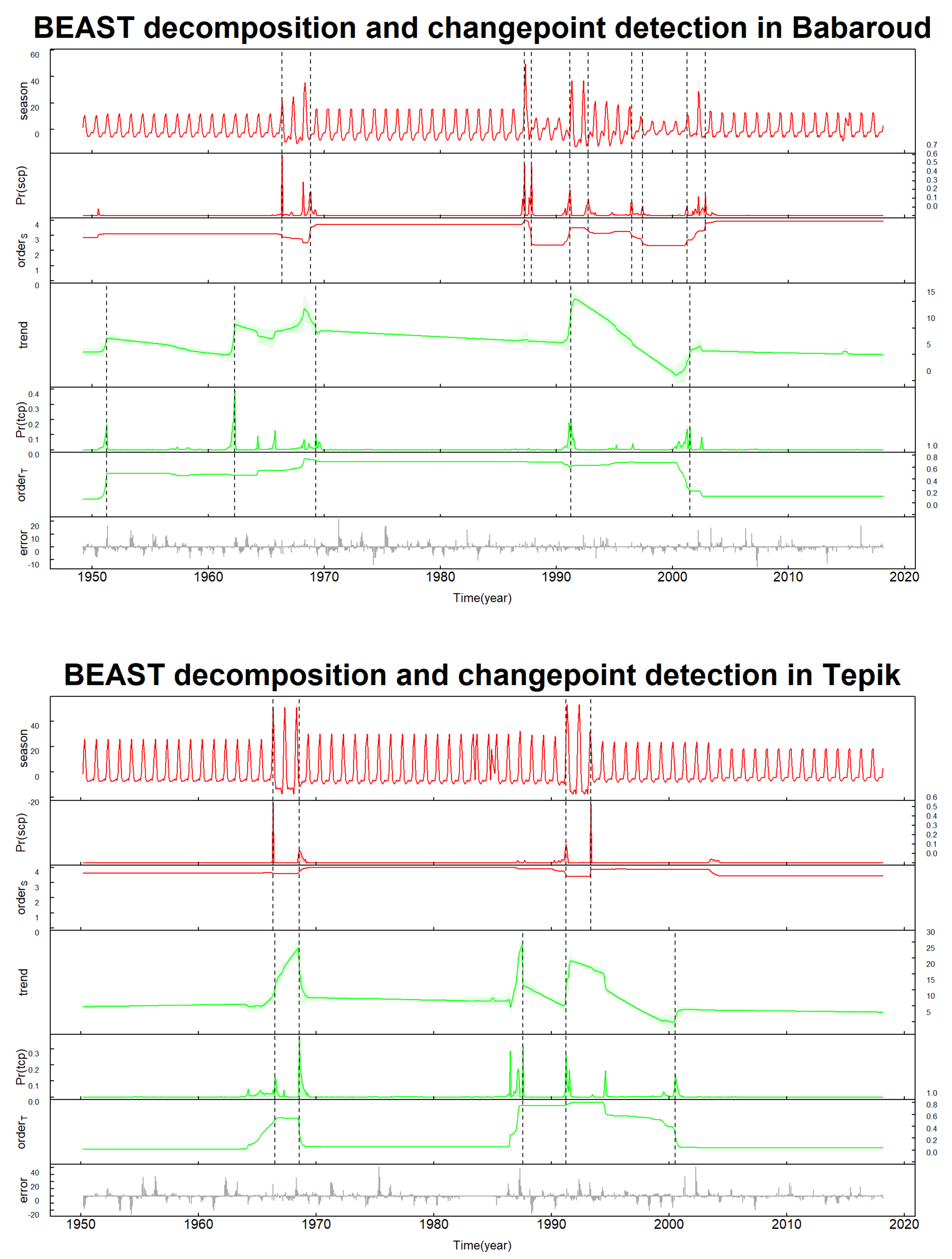
2.2. Trend and Change Point Analysis

The change point detection and nonlinear trend analysis were performed by a recently developed model known as BEAST [5]. The Bayesian decomposition algorithm employed in this study treats the time series as additive in nature at three major timescales, including (1) seasonality or periodic variations caused by intra-annual climatic variations; (2) gradual changes forced by long-term environmental trends such as climate change or drought; and (3) abrupt changes related to severe disturbances such as a flood. The time series is decomposed as the sum of the first two components; however, abrupt changes are embedded in seasonality and trends, and do not appear explicitly in the respective time series. Despite the conventional methods of trend analysis, in the Bayesian algorithm applied in the BEAST, an ensemble of single models is employed for decomposition of the trend. Due to model averaging, the resultant model is stronger than single weak models. Another redeeming feature of this method is the ability to characterize the uncertainty of the identified trend and seasonal change points by treating each unknown as a random variable, thus enabling it to evaluate how probable each point is to be a true model [22]. The mathematical background of BEAST is complicated and fully covered by Zhao et al. [5] for interested readers. However, in short, the response time series (yi) (e.g., flowrate), can be decomposed as follows:
y i = S ( t i ; Θ S ) + T ( t i ; Θ T ) + ε i
where S(.) and T (.) represent the seasonal and trend components, and ti denotes the time. The change points are implicitly embedded in the seasonal and trend components represented by the parameters Θ S and Θ T , which imply the locations and numbers of change points in the seasonal and trend part of the time series, and ε i is the error (noise) term with the respective mean and unknown variance of 0 and δ 2 ( N = ( 0 , δ 2 ) ). The Bayes’ theorem is employed to find the unknown parameters M = Θ T , Θ S , δ 2 as a posterior probability distribution simulated by Markov Chain Monte Carlo (MCMC) sampling as follows [5]:
f ( M | Y ) f ( Y | M ) f ( M )
This method has been successfully applied for detecting the long-term trend in stream water quality data [6] and identifying fine-scale human disturbance at the basin scale [22]. That being said, there was not any earlier application of this approach for the time series analysis of river flow to the best of the authors’ knowledge. The R statistical software was employed for time series decomposition in this research [5,22,23].

2.3. Hydrologic Simulation by SWAT Model

As a physically based, distributed, agro-hydrological model that operates on daily time scales (at minimum), the Soil and Water Assessment Tool (SWAT) [24] can primarily be applied to assess hydrology and water quality in agricultural catchments. The SWAT has been extensively used to evaluate hydrologic and LULC changes in the Middle East and worldwide [25,26,27]. The hydrologic modelling component of the SWAT is based on a modified version of the Soil Conservation Services (SCS) curve number (CN) method [28], in which the watershed is discretized into sub-basins and then into hydrologic response units (HRUs) composed of homogeneous land use and land cover (LULC), soil type, and slope. The daily precipitation volume is first subdivided into infiltration, surface runoff, and surface interception. In this respect, the runoff is estimated from precipitation according to the CN value (a dimensionless number fluctuating between 0 and 100) which is worked out based on soil properties, vegetative cover, and surface treatment of the respective HRU [29,30]. The CN number is then modified on a daily basis as a function of antecedent soil moisture content. Depending on the characteristics of the watershed, the surface runoff is routed into streams, ponds, and reservoirs within the respective sub-basins, whereas infiltration is divided into plant uptake, shallow and deep groundwater recharge, lateral flow, and soil evaporation. Part of the infiltration returns to surface waters as baseflow that, along with the surface water, is routed from sub-basins to the watershed outlet. In summary, the hydrologic cycle in the SWAT model can be specified following Neitsch et al. [31] as:
S W t = S W 0 + i = 1 t ( R d a y Q s u r f E a W s e e p Q g w )
where S W t and S W 0 represent the final and initial soil water content (mm) on day i, and t denotes the time step (day). R d a y is the precipitation amount on day i (mm), Q s u r f implies the surface run-off on day i (mm), E a is the evapotranspiration amount on day i (mm), W s e e p represents percolation or water entering the vadose zone from the soil profile on day i (mm), and Q g w demonstrates groundwater flow (baseflow) amounts on day i (mm). The water yield (WYLD (mm)) is the aggregate total amount of water leaving the HRUs and entering the main channel during the time step and is regarded as one of the critical parameters evaluated for the sustainable water resource management of the study area [32]. Mathematically, it can be calculated by the SWAT model following Arnold et al. [33] as:
W Y L D = Q s u r f + Q g w + Q l a t T l o s s
where Q l a t is the lateral flow (mm), and T l o s s represents the transmission loss from the system (mm). More specifically, in this study, the modelling using the SWAT was implemented using the 2012 version of the Arc SWAT interface for the SWAT. In general, the SWAT model requires input from meteorological data, soil properties of the watershed, and topography, together with land use. The digital elevation model (DEM) with a resolution of 30 × 30 m was downloaded from the United States Geological Survey (USGS) at https://earthexplorer.usgs.gov/ (accessed on 20 July 2021). The slope map was then prepared based on the DEM to be used along with soil and land use for HRU creation. Meanwhile, the soil map was obtained from the Food and Agriculture Organization (FAO) soil data set available at https://www.fao.org/soils-portal/data-hub/en/ (accessed on 21 July 2021). The required weather data, spanning 35 years from 1979 to 2013, were downloaded from the Climate Forecast System Reanalysis (CFSR) Global Weather Data at: https://swat.tamu.edu/data/cfsr (accessed on 21 July 2021). The weather data comprised daily precipitation, wind speed, relative humidity, and solar radiation in the SWAT file format. Additionally, the land use of 1984 was the base map, which was prepared by a supervised classification of Landsat images according to region of interests (ROI) selected based on expert knowledge and field visit. The land use map was updated in 2013 using the SWAT-Landuse Update Tool (SWAT-LUT) developed by Moriasi et al. [34].
The LULC classes were chosen to correspond to the dominant land covers in the study area and consisted of croplands (agricultural fields, gardens), bare soil (open space, unused lands, others), water bodies (lakes, swamps), build-up areas (residential and commercial lands and settlements), grasslands (natural vegetation cover, grazing lands, others), and impervious surfaces (roads, streets).
During the calibration process, a category of 21 parameters were selected in accordance with the literature review [33,35,36] and dominant conditions of the study area. For instance, due to the fact that the area of study was mountainous, the snowmelt and elevation band parameters were included in the calibration parameters by following the calibration procedure applied by Grusson et al. [37] and Dhami et al. [38]. The calibration of streamflow in the SWAT was performed by SWAT-CUP software using the Sequential Uncertainty Fitting (SUFI-2) algorithm [39] through historical records at 6 hydrologic stations over the extent of the study area (Figure 1) with respect to the data in warm-up (1979–1981) and calibration (1981–2009) periods.
The elevation band parameters were first calibrated by fixing the elevation band parameters at their optimum values, and the snow melt parameters were calibrated simultaneously. The other calibration parameters (Table 1) were then modified iteratively for each sub-basin until a reasonable agreement was found between the observed and simulated streamflow for the respective sub-basins in terms of the coefficient of determination (R2) and Nash–Sutcliffe (NS).
Generally, NS varies between minus infinity and 1, while a NS value larger than 0.75 is regarded as very good, satisfactory when NS is between 0.36 and 0.75, and unsatisfactory when NS is lower than 0.36 [30]. The R2 varies between 0 and 1, with values close to 1 implying perfect model prediction. Following each calibration run, the sensitivity of the involved parameters was inspected in terms of the t-statistic and p-values using a global sensitivity analysis. Additionally, the uncertainty of the SWAT model’s simulations can be assessed by the values of the p-factor and r-factor. The p-factor indicates the percentage of measured data bracketed by the 95% prediction boundary (e.g., 95 PPU, which is obtained by applying a Latin hypercube sampling method in order to produce the final cumulative distribution of the model outputs). In contrast, the r-factor denotes the average width of the 95 PPU band divided by the standard deviation of the observed variable [40]. Both of the latest performance metrics vary between 0 and 1, with values closer to 1 implying higher model performance and efficiency [41]. Once the SWAT’s performance reached a certain acceptable level, the model was validated on data from the validation period (2010–2013) by the same range of parameters obtained in the calibration period. Following successful calibration and validation of the SWAT model, the amount of WYLD for each HRU and sub-basin were extracted in order to attribute the levels of WYLD to each LULC class. These results were then aggregated for subsequent analysis.

2.4. Multiple Linear Regression and Johnson–Neyman Interaction Analysis

A multiple linear regression was performed on log-transformed values of the WYLD as a response variable versus LULC classes, elevation, and an indicator of land-use intensity (La), which was closely related to LULC in the study region as explanatory variables to analyze their impact on fluctuations of water yield. The indicator of land-use intensity (La) [42] can be calculated as:
L a = 100 × i = 1 n A i C i       L a 100 , 400
where L a is the land use intensification degree related to each sub-basin, with values fluctuating between 100 and 400, in which larger values imply higher intensity of land resource use. A i is the corresponding grading index for the ith land use type regarding the categorization offered by Zhuang and Liu [42] as rendered in Table S1, C i is the percentage of ith land-use types in each sub-basin, and n represents the number of sub-basins in the study region.
The Durbin–Watson (DW) statistic along with variance inflation factor (VIF) were utilized to inspect the existence of autocorrelation in the residuals from the regression and multicollinearity among predictors, respectively. Due to high correlation among some explanatory variables, three regression models, including ridge regression (RR), lasso regression (LR), and elastic net regression (ENR), were carried out as alternative methods against the problem of multicollinearity. The performance of each of these regression models was investigated with the training and validation data in terms of the r-squared (R2) and root mean square error (RMSE).
On the other hand, the JN approach, which was performed following the multiple linear regression for analyzing the interactions of the LULCs on WYLD, is actually an extension of the traditional test of simple slopes for analyzing the conditional effect (e.g., effect of one variable over the values of another variable) of a focal predictor at specified values of a moderating variable, such as low, high, and medium. If it is a continuous variable, it is determined by computing a critical ratio (t) as follows [16]:
t = ω ^ V A R ^         ω ^ 1 2
where ω ^ and V A R ^     ω ^ are the conditional effect (Equation (7)) assigned as weighted linear composites of the random normal variates for parameter estimation of a fixed effect regression model and its associated variance (Equation (8)):
ω ^ = α 1 γ ^ 0 + α 2 γ ^ 1 + + α p γ ^ p 1 = α ´ γ ^
V A R ^         ω ^ = V A R ^   a ´ γ ^ = a   ´ A C O V ^ γ ^ a
where “ α ” is a p × 1 column vector containing the a 1 , a 2 , , a p fixed weights used to form the composite, γ is a p × 1 vector of fixed regression parameters relating each predictor to the criterion, and A C O V ^ γ ^ represents the sample estimate of the asymptotic covariance matrix of the regression coefficients. With this mathematical background in mind, the JN approach, on the other hand, requires estimation of the regions of significance instead of single values of the moderator, along with confidence bands, for the conditional effect. Indeed, the region of significance means detecting the range of the moderator over which the effect of the focal predictor is significantly positive, nonsignificant, or significantly negative. In this case, we solve for the values of the moderator that return a critical value of t c r i t , instead of t, as:
± t c r i t = ω ^ V A R ^         ω ^ 1 2
This value can turn into t 2 c r i t V A R ^   ω ^ ω ^ 2 by a simple manipulation. For the case of a simple two-way interaction, (e.g., the conditional effect of x1 given the values of x2), the two roots of the moderator that satisfy this equality can be solved by a quadratic formula as follows:
a x 2 2 + b x 2 + c = 0
a = t 2 c r i t V A R ^   γ 3 ^ γ 3 ^ 2
b = 2 t 2 c r i t C O V ^   γ 1 ^ , γ 3 ^ γ 1 ^ γ 3 ^
c = t 2 c r i t V A R ^   γ 1 ^ γ 1 ^ 2
By applying a quadratic formula, the values of x2 that satisfy the following equations can be obtained as:
x 2 = b ± b 2 4 a c 2 a
The two roots of Equation (14) return the boundaries of the regions of significance, while the formula for estimating the confidence band is:
C B ω ^ = ω ^ ± t c r i t V A R ^         ω ^ 1 2
All of the required codes in this part of the research were written in R statistical software [43].

3. Results and Discussion

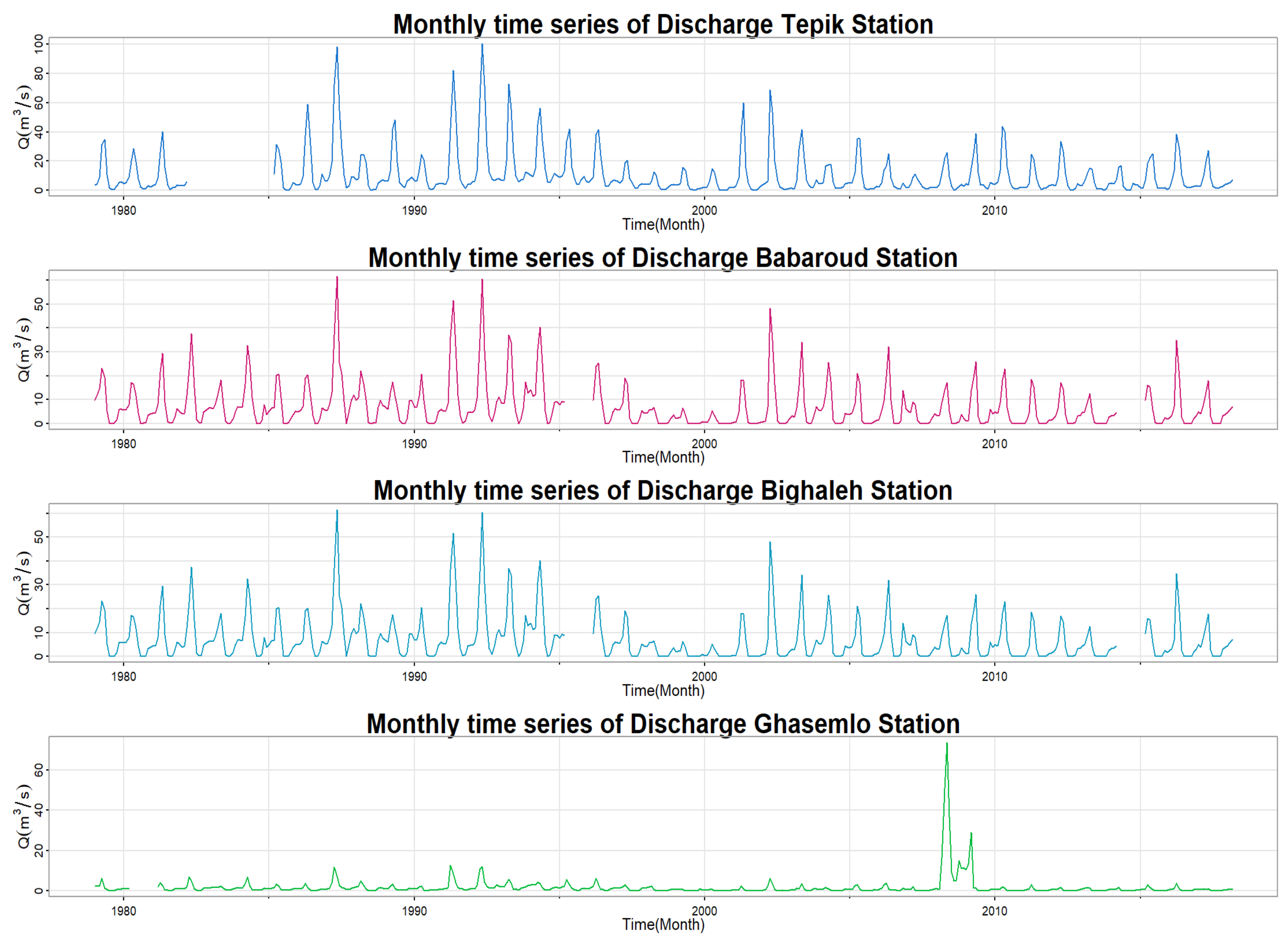
3.1. Trend Analysis of Stream Flow

The time series plots of four selected gauging stations in the study area are depicted in Figure 2. The location of these stations is illustrated in Figure 1.
Since the flow in all of these rivers discharge into Urmia Lake, the long-term fluctuations of flow have a direct effect on Urmia Lake water level variations accordingly. More specifically, the long-term trend of the three top stations (Tepik, Babaroud and Bighaleh) were similar to each other, which indicates the influence of the same external factors on these stations, despite the fact that they are located in different sub-basins. There were higher levels of discharge in Tepik station, with peak values exceeding 80 m3/s, whereas the maximum recorded values of discharge were 60 m3/s in Babaroud and Bighaleh. Tepik resides in an upstream part of agricultural fields, while the latest stations are in the downstream part of agricultural lands, which implies the high rate of water consumption in agricultural sector. Another point worth noting is the significant decrease in water inflow since 2010, with peak values hardly ever approaching 40 m3/s for all the considered stations. Due to the fact that the Tepik and Babaroud stations had the longest and most complete discharge records, they were further processed by the BEAST’s time series decomposition for change point detection.
As can be seen, the streamflow records were in the historical range of 1949–2018 (e.g., 70 years) for Babaroud and 1950–2018 (e.g., 69 years) for Tepik (Figure 2). Meanwhile, Table 2 contains the list of probable trend and seasonal change points. The time series decomposition implemented by the BEAST consisted of eight different panels (Figure 3).
The top panel represents the observed steam flow (blank circles), the fitted time series (black line), and the 95% credible interval obtained by Bayesian simulation, which is highlighted with a gray band. The second and third panel indicate the seasonal component and its respective probabilities. In this respect, the order in Figure 3 shows the estimated mean order of the piecewise polynomials required to adequately fit the trend. An order close to 1 means a linear trend, while values close to 0 implies a flat trend. Likewise, orders implies the order of a seasonal component if any periodic variation is being detected in the flow rate. The trend component and its associated probabilities were depicted in the fifth and sixth panel, whereas the last panel demonstrates the error term ( ε i ) as explained in Equation (1). In this context, the most probable seasonal and trend change points have been illustrated by vertical dashed lines in the respective panels.
Regarding the panel of trend change points, five change points (abrupt changes) can be detected. The r-squared (R2) and root mean square error (RMSE) of the Bayesian’s model were 0.82 and 6.34 for Tepik compared to 0.85 and 3.57 for Babaroud, which indicates the outperformance of the model fitted to Babaroud station. The probability distribution of having a change point in the trend at each respective point for Tepik demonstrated that there were two most probable change points in 1968 and 1991, with associated probabilities of 0.99 and 0.65. The other detected change points in 2000, 1987, and 1965 are less likely to be significant change points, as their respective probabilities were 0.43, 0.41 and 0.35 (Table 2).
The most probable change points for Babaroud were in 1991 (cpPr = 0.97) and 2000 (cpPr = 0.75), while the other three change points in 1969 (cpPr = 0.65), 1958 (cpPr = 0.61) and 1964 (cpPr = 0.55) had significantly lower probabilities to be regarded as abrupt changes. Both stations had the year 1991 in common with each other as one of the most likely change points. On the other hand, Urmia Lake’s water level started to decrease sharply from 1995 [44], which indicates that part of this decline was most probably caused by stream flow decrease within a 4-year time delay. Accordingly, for the case of Tepik and Babaroud, a linear decreasing trend (orderT) is expected to have taken place between 1991 and 2000 (e.g., location of probable change points highlighted with vertical dashed lines).
Some recent studies indicate that there has been a significant decline in the water level of Urmia Lake since 2000, which was attributed to agricultural expansion [45]. The decrease in water inflow to Urmia Lake because of water overexploitation from discharging rivers like Babaroud and Tepik might also be a contributing factor for this phenomenon.
A linear increasing trend was observed between 1965 and 1968 in the Tepik station. A similar increasing trend was detected between 1958 and 1964 and between 1964 and 1969 in the Babaroud station. Part of the latest growing trend of streamflow coincided with the same trend in the Tepik station, which implies that these rising or falling trends might have been influenced by similar external factors, such as higher precipitation during these time periods. Since 2001, a flat trend can be identified in both stations, which was stable up to 2018. This trend was the lowest detected level of streamflow during this 70-year time period. Additionally, there were some probable seasonal change points highlighted in Pr(scp) in both Figures. The main differences were the higher number of seasonal change points in Babaroud compared to those of Tepik and the larger average harmonic order required to approximate the seasonal component (orders) in the Tepik station.
Part of the findings of the current research are in line with the results of Nikbakht et al. [20], who conducted research on the streamflow drought severity in Urmia Lake Basin (ULB) based on the analysis of 14 hydrometric stations, since they demonstrated that the worst streamflow droughts in almost all the stations occurred from 1999–2000 and from 2000–2001.
This significant decrease in the level of streamflow was also easily detectable in the BEAST’s decomposition trend in the current research. On the other hand, in a similar study performed by Nazeri Tahroudi et al. [19] on the long-term trend of 25 hydrometric stations in ULB using the Mann–Kendall test, it was concluded that the time of change point of river flow was between 1994 and 1998 exactly 2 years following the change point in the precipitation series.

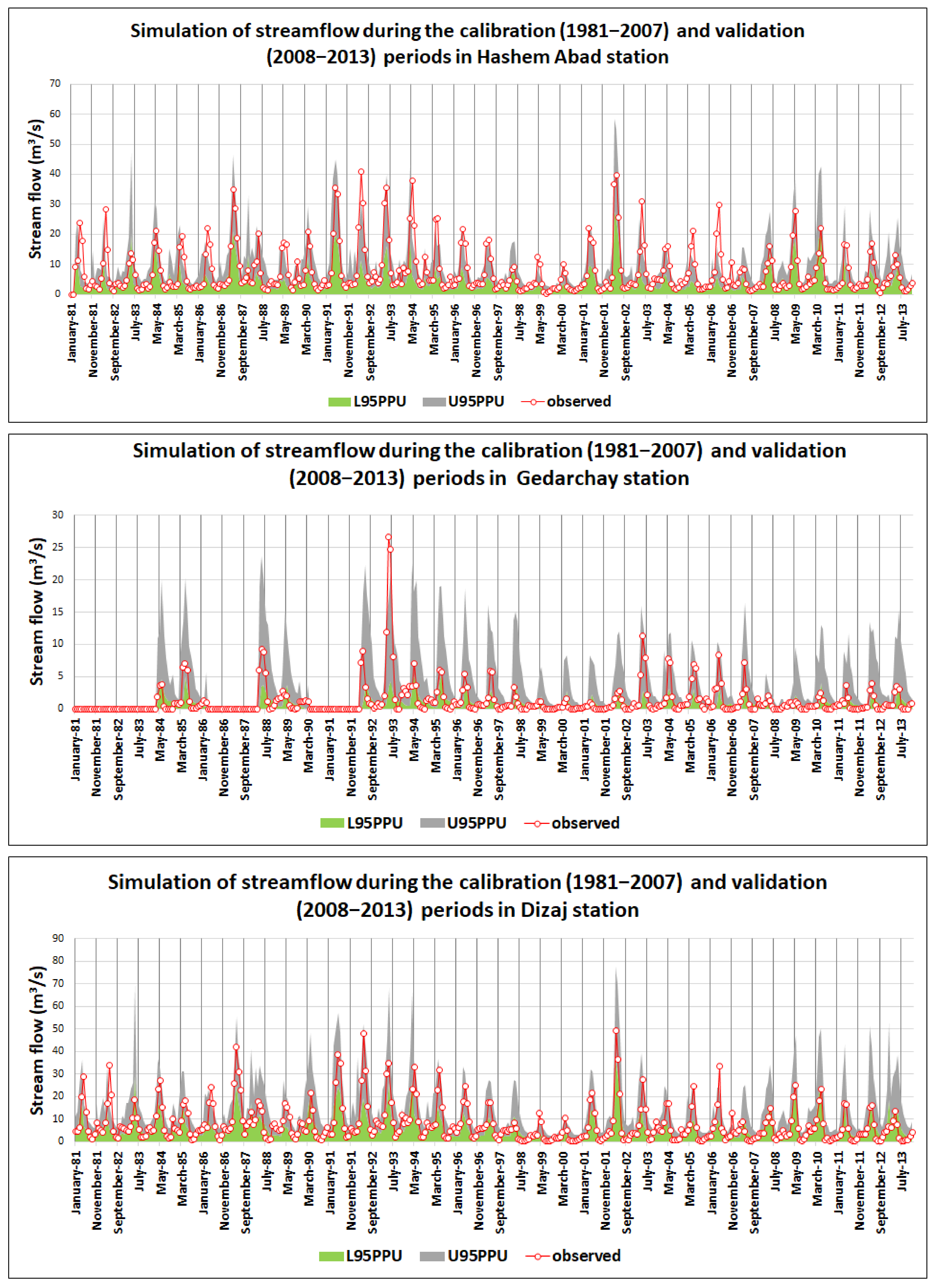
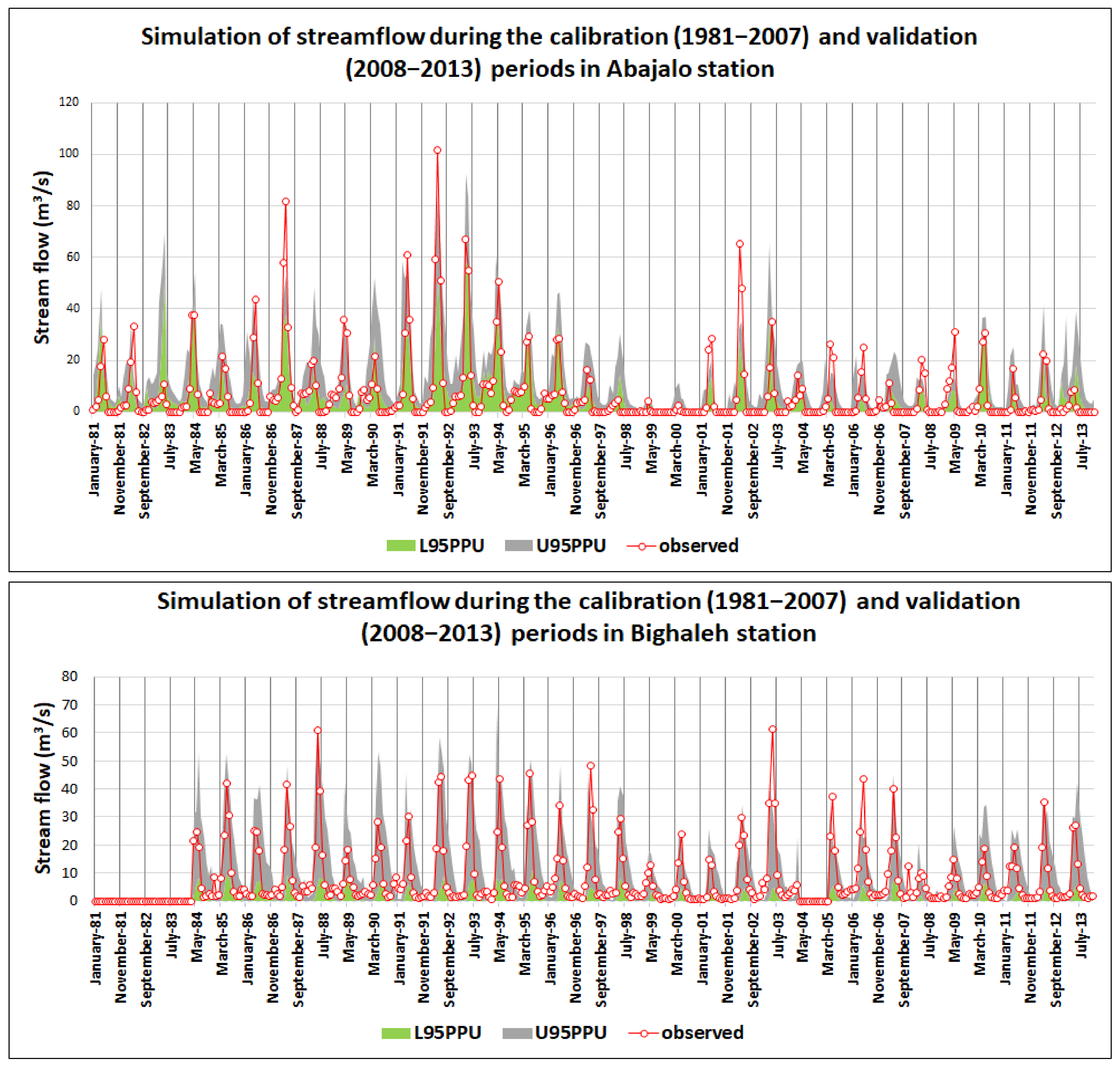
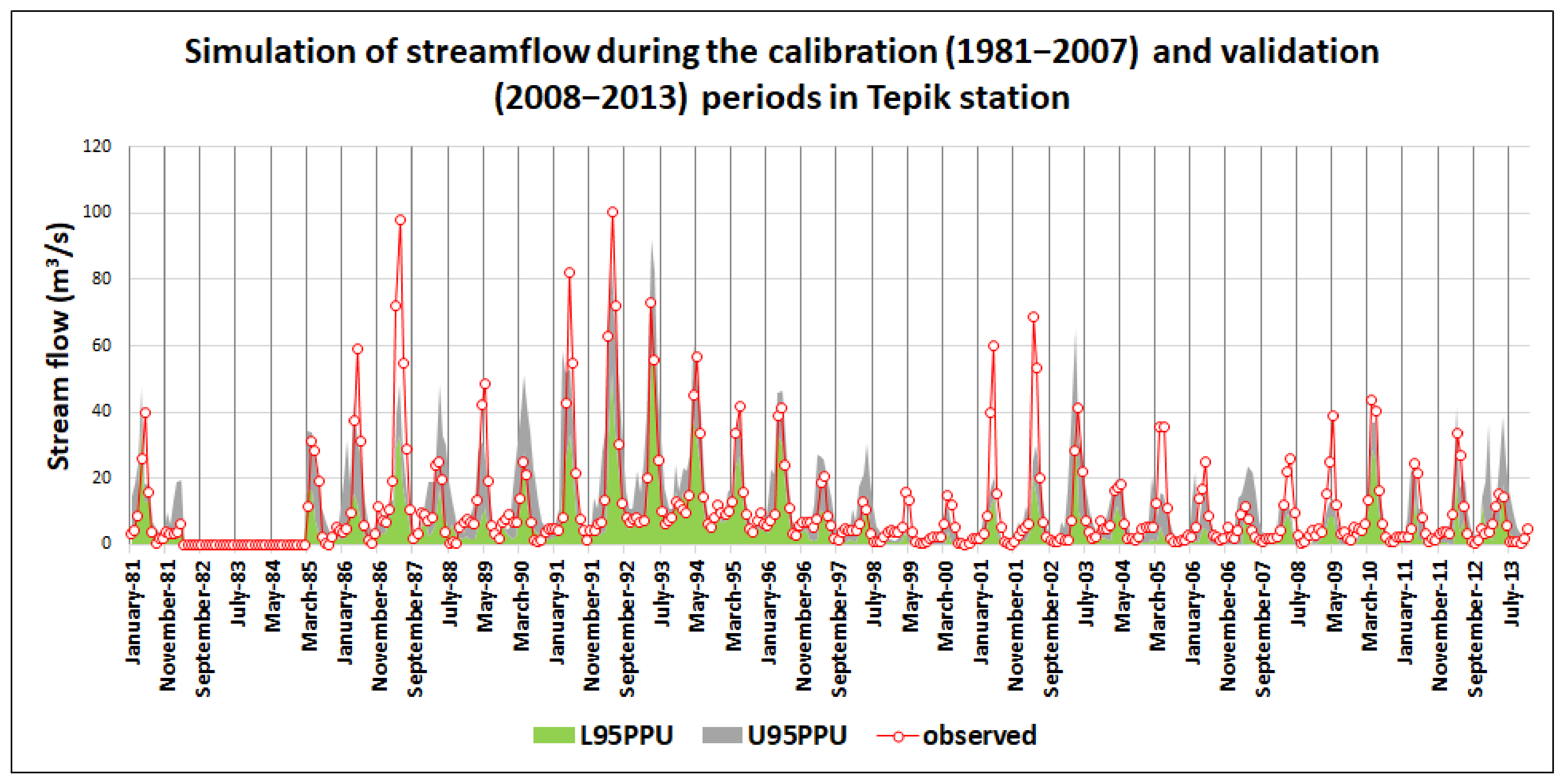
3.2. Water Yield Estimation by the SWAT Model

The SWAT’s calibration parameters, along with specified ranges and fitted values, are given in Table 1. It should be noted that, other than the elevation band and snow melt parameters, the final fitted values for other parameters varied for each sub-basin, because the upstream sub-basins of each of the six hydrometric stations were calibrated separately. Regarding the results of the global sensitivity analysis performed after each calibration run, it turned out that the CN2 (runoff curve number) and SOL_AWC (available water capacity of the soil layer) were the most sensitive and influential parameters on fluctuations in streamflow. The former parameter is a function of soil permeability, land use, and antecedent soil water conditions, thereby making it very important for the accurate estimation of surface runoff. This finding is consistent with the results of many other studies around the world [46,47,48]. For instance, Nossent et al. [49] performed research investigating the sensitivity of the SWAT’s major parameters using Sobel’s sensitivity analysis. It was found that the curve number (CN2) was by far the most important parameter in that about 65% of the variations in the simulated stream flow were caused by fluctuations in CN2, either directly by the variation of the parameter itself (25%) or by interactions with other parameters. Similarly, in research conducted by Kushwaha and Jain [50] in India, the CN2 turned out to be the most sensitive parameter influencing water yield. More specifically, in the latest study, the CN2 received the highest rank among the parameters affecting stream flow, whereas the SOL_AWC was identified as the most sensitive parameter influencing the base flow. This is also consistent with the results in our current research. Xueman et al. [51] further indicated that the CN2 and SOL_AWC were not only the most sensitive parameters controlling surface runoff, but also their interaction had a major effect on the average annual runoff.
The performance metrics associated with the calibration and validation data in terms of R2 and NS are rendered in Table 3. Considering the calibration data, all of the hydrometric stations produced R2 values larger than 0.5, which indicates satisfactory results. In particular, other than the Gedarchay station in the downstream part of the watershed yielding an R2 of 0.57, the amounts of R2 for all of the other stations were larger than 0.6. The best results were obtained for the Bighaleh and Abajalo stations, with R2 values of 0.75 and 0.68, respectively. The spatial locations of these stations can be found in Figure 1. The latest performance metric denotes the proportion of variation explained by the model. For instance, regarding the Bighaleh and Abajalo stations, 75% and 68% of the variation in calibration time series could be explained by the SWAT model. The validation time series implies the generalization ability of the model for other hydrometeorological conditions. Therefore, a model with high performance for both calibration and validation data can be applied for the prediction of future conditions. In this case, other than the Tepik station yielding a lower R2 (0.49), the amount of R2 for all of the stations during the validation period were higher than 0.6, and the best results were obtained for Bighaleh, Hashem Abad, and Dizaj, with R2 values of 0.73, 0.73 and 0.72, respectively.
On the other hand, with respect to the NS of the calibration data, the best results were yielded for Bighaleh (0.74), Abajalo (0.68), and Dizaj (0.66), whereas the NS values for Tepik (0.49) and Gedarchay (0.47) were accordingly lower. The respective NS of Tepik and Gedarchay for the validation data were 0.37 and 0.52, respectively. Accordingly, the NS values of all of the simulated stations were larger than the cut-off value of 0.36 set by Oeurng et al. [30]. As mentioned earlier, the results of the SWAT model are regarded as satisfactory when NS varies between 0.36 and 0.75 [30]. Due to the fact that these hydrologic stations are located in the lower, middle, and upper parts of the watershed (Figure 1), it confirms the fact that the model succeeded to simulate streamflow for the whole basin.
Meanwhile, the uncertainty of the model predictions can be assessed by the p-factor and r-factor, which indicate the percentage of the observed data bracketed by the 95 PPU band and the average thickness of the 95 PPU band divided by the standard deviation of the measured data, respectively [52]. Regarding the results (Table 3), and, with respect to the fact that we are looking for a balance between p-factor and r-factor, the lowest model uncertainties were associated with Bighaleh station, which contained the respective p-factor and r-factor of 0.57 and 0.81 for the calibration data compared to 0.50 and 0.72 for the validation part. On the contrary, there was a high uncertainty attributable to the validation results in the Dizaj station, which yielded a p-factor and an r-factor of 0.29 and 0.47, respectively.
The graphical results of the SWAT model simulations can further depict the trend of observed streamflow for the calibration (1981–2007) and validation (2008–2013) part, together with the uncertainties rendered by the upper 95 PPU (e.g., 97.5% level obtained by the Latin Hypercube sample of 95 PPU), and the lower 95 PPU (e.g., 2.5% level obtained by the Latin Hypercube sample of 95 PPU) (Figure 4). In summary, there were uncertainties of model predictions for some peak flows. As a whole, other than some time periods, the SWAT model’s simulations could capture the trend of observed values reasonably well.

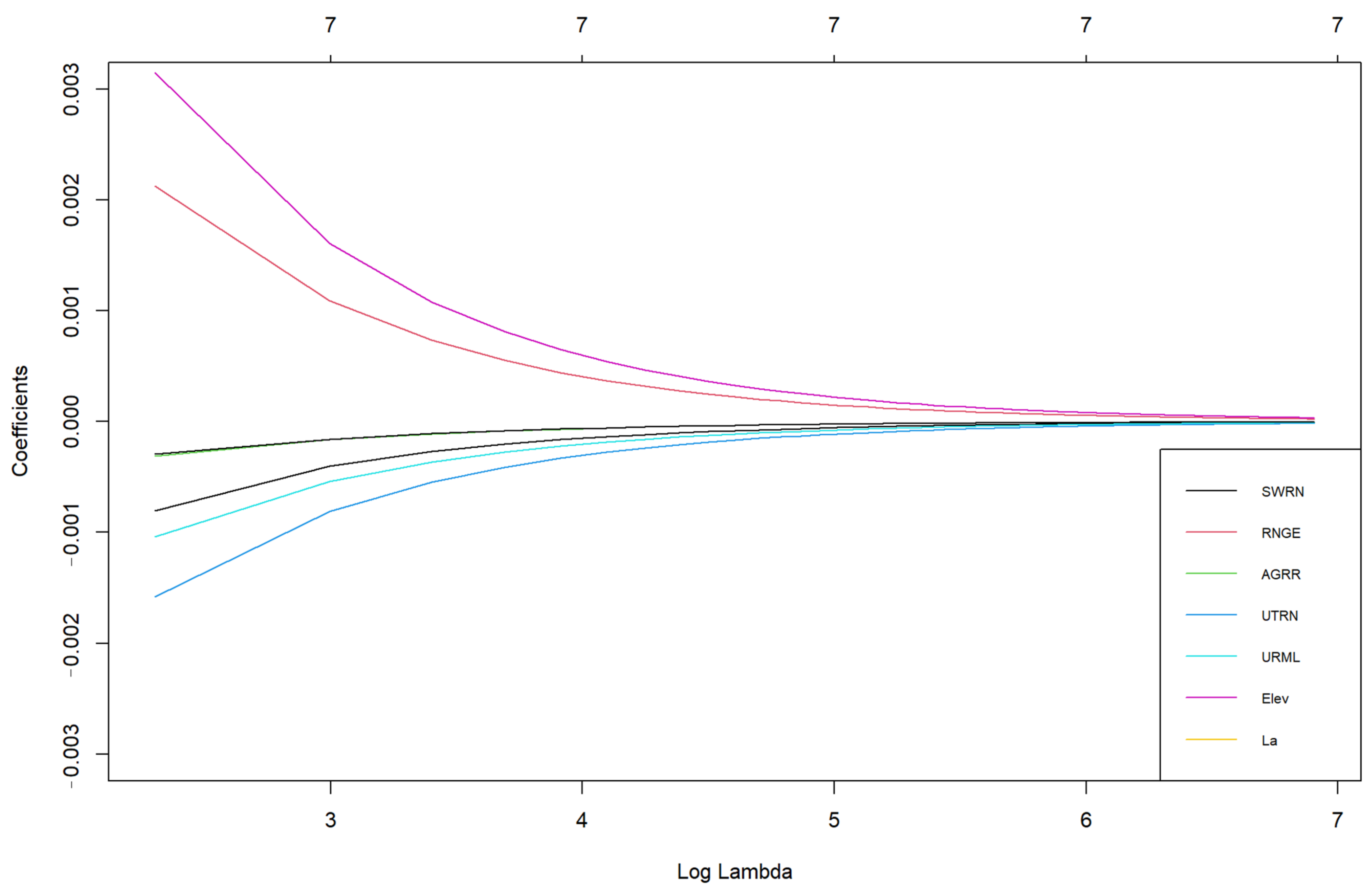
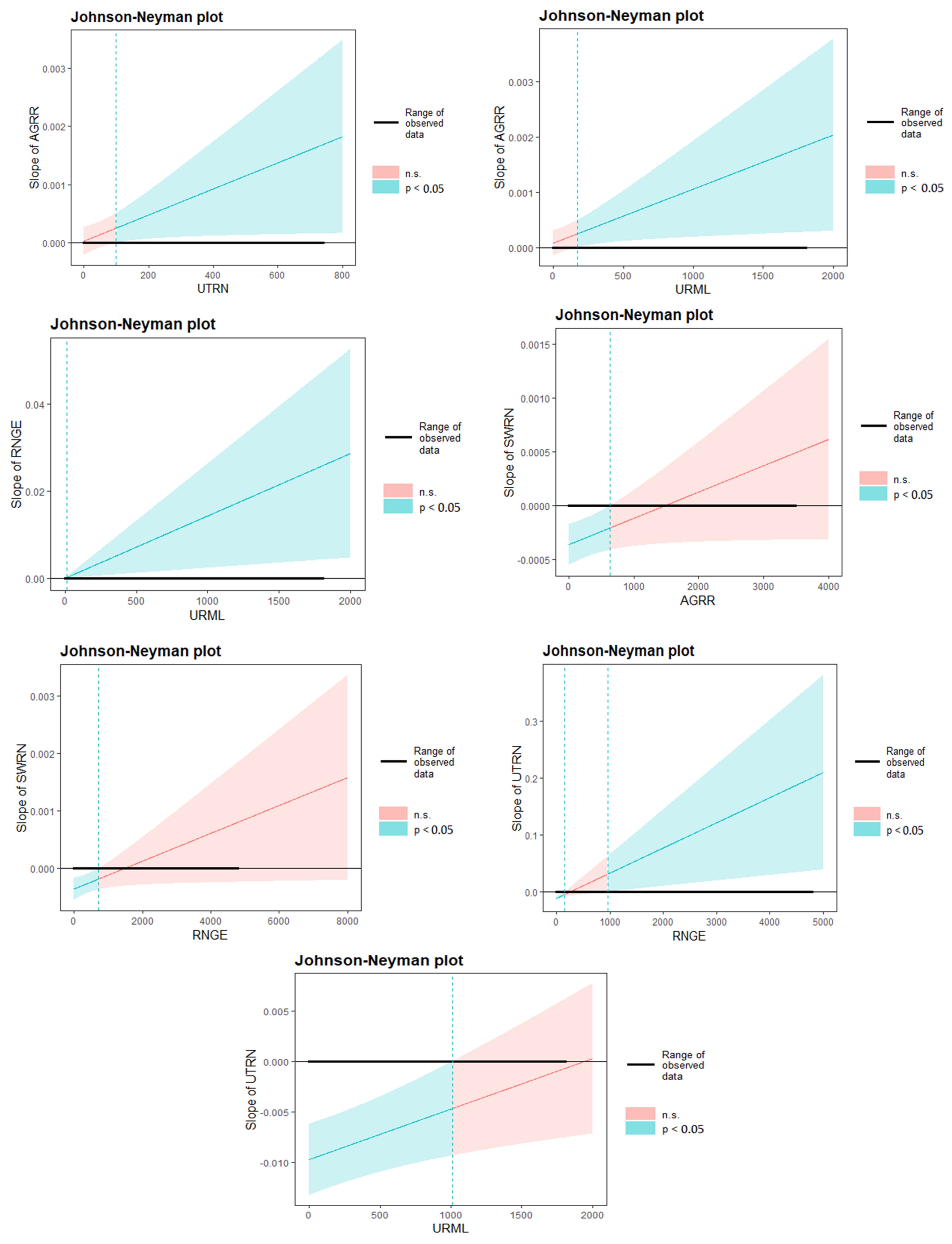
3.3. Main and Interaction Effects of LULCs on Water Yield

A multiple linear regression (MLR) was applied to the SWAT’s model results in order to identify the contribution of major land covers (e.g., the area of each land cover in sub-basins), together with the elevation and indicator of land-use intensity (La), as predictors of water yield as a response variable. In this case, only the main effect and two-way interactions of explanatory variables were taken into account. The diagnostic plots depicted in Figure S1 provide a graphical approach to determine whether assumptions of the MLR (e.g., linearity of data, normality of residuals, homogeneity of variance, independence of residuals) have been met, and also to identify outliers (problematic influential data points) affecting the regression model. In particular, the correlation between residuals and fitted values (top left panel) highlighted a trend indicating that some outliers might be problematic for the model. However, the linearity assumption between predictors and outcome was met though sub-basin numbers 322, 288, and 252, can be regarded as outliers based on the information provided in this panel. These statistical issues will be addressed in the following paragraphs.
The normality of residuals (as one of the main assumptions of the regression model) can be tested by the normal Q–Q plots (top right panel). When the points lie on the line, it indicates that the normality of residuals has been met. In this case, except for some lower and upper mediate points, all of the other data were on the line, which indicates that the normality assumption had been met, but the model may have had difficulty in predicting some small and large values. Additionally, the graph of squared absolute standardized residuals versus fitted values (bottom left) implies valuable information about homogeneity of variance (homoscedasticity). More specifically, the lack of a significant trend indicates that the variance of residuals remained constant and did not correlate with any predictors. The homogeneity of variance was further tested by Durbin–Watson (D-W) statistic, which varies between 0 and 4, where a value close to 2 and a non-significant result imply that the null hypothesis of non-existence of first-order autocorrelation should be accepted, and the homogeneity of variance was met. Meanwhile, the D-W statistic was 2.15 with a p-value of 0.25, which demonstrates that there was no statistical evidence of autocorrelation in the residuals. Finally, the plot of residuals and leverage (bottom right) can help to identify possible outliers having the potential to disproportionately affect the regression results. As suggested by Gareth et al. [53], data points with absolute standardized residuals greater than 3 can be regarded as possible outliers, which suggests that none of the points were a substantial outlier. Additionally, according to Field et al. [54], the observations for which Cook’s distances are greater than 1 are problematic and can be removed. Accordingly, only one data (e.g., 133) was problematic and could be omitted. The last prerequisite test was collinearity analysis between independent variables based on the variance inflation factor (VIF), the results of which are depicted in Table S2. These findings imply that a large number of predictors (either the main effects or their 2-way interactions) had VIFs exceeding 5 [55], which indicates the presence of multicollinearity that can lead to larger values of standard errors of estimates and confidence intervals, thereby obscuring the interpretation of the results [56].
In the presence of multicollinearity, one option is to remove variables contributing to collinearity, while another option is to reassess the data using the methods that are robust against collinearity. The last option is to employ dimensionality reduction techniques. Correspondingly, the first two options were applied in the current research by using regression methods to avoid the problem of collinearity and removing variables contributing the most to collinearity. For this purpose, ridge regression (RR), elastic net regression (ENR), and lasso regression (LR) were employed as alternative methods for which the results of the performance metrics on the training (70%) and validation (30%) data are rendered in Table S3. In terms of R2 and RMSE, both RR and ENR produced very similar results for the training and validation data set. In particular, the R2 values associated with the latest methods were 0.20 and 0.27 for the training and validation part. In other words, these models were able to explain 20 and 27 percent of the variance of WYLD within the extent of the study area by only accounting for the dominant land use and land covers (LULCs), along with the elevation and index of land use intensification (La). It should be noted that we have not considered some more important parameters, including climatic variables such as precipitation and temperature, in our calculations. In spite of the fact that fluctuations in climate variables and the LULC are the primary drivers of water yield, the intensity of effect for climatic parameters (especially rainfall and evapotranspiration) on WYLD seems to be more significant than that of the LULC [57], which can justify the low values of R2 produced in this part of the research.
Moreover, regarding the RMSE, again, both RR and ENR generated very similar results. In other words, there were some minor dissimilarities between RR and ENR models, with RMSE values of 20.36 and 20.14 for the training versus 19.74 and 19.37 for the validation part, respectively. The outperformance of these models for the validation part indicates the out-of-sample generalization abilities of the respective regression models. The LR model, on the other hand, exhibited a slightly lower performance for the training and validation part, with respective R2 values of 0.18 and 0.22 compared to the RMSE of 22.05 and 21.69, which indicated that the higher accuracy of model for validation data in comparison with the training set was still the case. In order to further investigate the influence of each LULC class, together with the elevation and La index, on WYLD at sub-basin level, the trend of the lambda parameter (in log scale) was investigated against the coefficients of the ridge regression as one of the best performed models (Figure 5). It should be noted that, for better interpretation, only the main effect of the predictors was investigated in these regression models.
It can be seen that, when the log of lambda rose, the magnitude of coefficients decreased toward zero. That is because of the uniform penalties given to predictors by ridge regression (through shrinkage of the absolute values of coefficients toward zero) to prevent multicollinearity and to reduce model complexity. The regularization term applied in lasso and ridge regression can not only obviate the problem of multicollinearity (high correlation between predictors), but also the problem of outliers (high biases) is alleviated by balancing the trade-off between the variance and bias [58]. Therefore, the issues identified in diagnostic plots (Figure S1) can be obviated by applying the foregoing regression models.
In this regard, elevation and rangeland had a strong predictive power for WYLD with a positive linear relationship, while road (UTRN) and settlement (URML) classes exhibited the most inverse effect on the decrease in WYLD within the area of study (Figure 5). Agriculture (AGRR), along with the land use intensification index (La), demonstrated similar minor effects on water yield that were indistinguishable from each other, which indicated a similarity in intensity of their effects on WYLD. This shows that agricultural land use has had a significant effect on land use development among the investigated sub-basins. In contrast, the soil class (SWRN) had an intermediate negative effect on water yield.
In the references, the most widely applied model for analysis of the impacts of land use and land covers on water yield was the Integrated Valuation of Ecosystem Services and Tradeoffs (InVEST) water yield model [59,60,61]. However, the InVEST model does not make a distinction between surface and groundwater resources, which can be regarded as the main disadvantage associated with this model that results in inaccurate estimation of the hydrologic components [57]. In contrast, the SWAT model can differentiate between the surface and groundwater flow; therefore, hydrologic components are more accurately estimated in this model. Dennedy-Frank et al. [62] investigated the efficiency of the InVEST and SWAT model at two watersheds in the USA and concluded that the spatial distribution of water yield estimated by the InVEST model may be less accurate than that of the SWAT model due to not accounting for the baseflow in calculations, which was a significant proportion of their study area’s total water yield.
The results of this study regarding the fact that a decline in vegetated land can lead to increase in WYLD are consistent with the finding of Li et al. [63], who performed their study in the Jing-Jin-Ji region, China. In addition, the findings of the latest study were also in agreement with those obtained in current research indicating that vegetated lands have low WYLD coefficients, which can be attributed to the higher rates of evapotranspiration and water infiltration associated with this land use class. Nonetheless, water yield coefficients of vegetated areas in Citarum River Basin, Indonesia [57] were larger than that of build-up and bare soil lands, which is not in agreement with the findings of the current study. In spite of this, the latest research reached a similar conclusion to the current study that the expansion of open lands (e.g., bare soil) can result in a decrease in water yield. Likewise, the study conducted by Li et al. [63] confirmed the high WYLD coefficient of settlement class; however, it was found that expansion of the built-up area could increase total water yield, which is not in line with the results of the current study.
As mentioned earlier, another alternative option against the problem of multicollinearity is to remove independent variables with significant multilinearity [55]. In this respect, following the removal of the explanatory variables contributing most to the multicollinearity, a multiple linear regression was performed on a reduced number of predictors. The main effects, together with two-way interaction terms associated with VIF, were inspected to make sure that the multicollinearity problem between explanatory variables had been obviated. Then, the Johnson–Neyman (JN) technique [64] was utilized in a multiple regression framework to investigate the conditional interactions between LULC and their effect on water yield. It is noteworthy that by interaction we mean that the linear relationship between the dependent variable and predictor is affected by another explanatory variable (e.g., moderator).
More specifically, the JN approach would estimate the statistical range of a specific LULC over which the relationship between another LULC and WYLD is significant. This is a quantitative procedure to identify the two LULC areas where the 95% confidence interval for the LULC–WYLD relationship is equal to zero. That is to say, within this mean range, the LULC–WYLD relationship is statistically significant (at 95% confidence level); whereas outside this mean range, the relationship is not statistically significant [65]. Ultimately, regions of significance are provided by the JN method where the explanatory variable (LULC) predicts the response variable (water yield) over the range of the moderating variable (another LULC) [66]; thereby, the interactions of respective LULCs on WYLD can be quantified.
The results of the JN procedure are depicted in Figure 6 only for the statistically significant interactions (at 95% confidence interval) based on the results of multiple linear regression.
Each JN plot contains a WYLD coefficient associated with the respective LULC on the y-axis. This represents the influence of that LULC on WYLD fluctuations against the range of a moderator variable (e.g., another LULC) illustrated on the x-axis, which implies the area of moderator LULC in this case. Additionally, each panel has a 95% significant confidence bound, along with a nonsignificant confidence bound, demonstrated by the cyan and pink colors showing the trend of simulation. In each figure, the vertical dashed line separates the boundary between significant and nonsignificant levels, while the thick horizontal line indicates the range of observed data. It should be noted that the results of the Johnson–Neyman plot may not be statistically interpretable for the values outside the range of observed data.
Regarding the results in each sub-basin, the effect of soil class (SWRN) on water yield was statistically significant only when the area of rangeland (RNGE) was less than 717 ha and the area of agricultural land was less than 633 ha. Given the fact that the effect of SWRN on WYLD was significantly negative in both cases, and the range of observed values of SWRN overlapped with the significant bound, this indicates that there was a significant and negative relation between soil class and water yield. Meanwhile, the confidence bands indicate that the conditional effect of soil on water yield was estimated with the most precision at lower areas of rangeland and agriculture, while the precision was decreasing at medium and high areas of moderating LULC classes, as represented in a large confidence interval. This conclusion was the case for all of the other Johnson–Neyman plots. For all of the plots, some parts of high quantile estimations resided outside the range of observed data (depicted by thick black line), which indicates that this part may not be statistically interpretable.
On the contrary, in the investigated sub-basins, the impact of road class (UTRN) on water yield was statistically significant (95% confidence level) only when the area of rangeland was lower than 152 ha and larger than 960 ha. When the size of rangelands varied between 152 ha and 960 ha, this effect was statistically non-significant. Additionally, our results indicated that the conditional effect of UTRN on WYLD was significantly negative at settlement areas lower than 1013 ha, while nonsignificant at settlement areas between 1013 and 1807 ha. The agricultural class had a statistically significant effect on water yield only when the area of road and build-up exceeded 100 and 170 ha, respectively. Finally, when the area of settlements in sub-basins was larger than 11 ha, the effect of rangeland on WYLD was statistically significant.
This study was the first application of the Johnson–Neyman approach for analyzing the two-way interactions of LULC on water yield at the sub-basin scale in hydrologic and environmental sciences. In similar research, Xiong et al. [67] considered the interaction effects of climate (temperature and precipitation) as well as land use and land cover on soil organic carbon sequestration by using the inclusion of a cross-effect term in the general linear model. The same procedure using general linear models was followed by Molina et al. [68] to assess the interaction effect of LULC and vegetation cover on runoff generation.
There are some obvious redeeming features associated with JN method compared to the traditional methods, such as simple slope. Firstly, the slope of a focal predictor can be assessed over the entire range of the moderating variable instead of a small number of values. In fact, the JN approach implicitly contains the results of simple slopes analysis. Secondly, regions of significance can be provided for the two-way interactions of the focal predictor and moderator on the response variable. Thirdly, the precision of the effect of the focal predictor over the full range of the moderator can be graphically depicted, where, in narrow regions of the confidence band, the conditional effect of the focal predictor on the outcome can be estimated with the most confidence and vice versa. Fourthly, despite the fact that one of the assumptions of regression models is that the explanatory variables are known and fixed values measured without error (e.g., predictors are non-stochastic), the JN approach is robust against the violation of this assumption. The results are reliable even for stochastic predictors, since measurement errors cause shrinkage of the region of significance and reflect in a broad confidence band.
However, as stated by Bauer and Curran [39], there are some limitations associated with this method, as well. In situations when the multiple linear regression model assumptions are violated, the variances of the model are not correctly specified. For instance, this situation occurs when explanatory variables contain a high degree of collinearity, when the distribution of residuals of the model is not normal, and when the homogeneity of variance is not met. That is why we should be careful about interpretation of regression results when any of the underlying assumptions are violated. Another limitation of the JN method is that only two-way interactions between the focal predictor and moderator can be estimated, whereas, at least for our case, the interaction between LULCs within each sub-basin might be too complicated to be limited to only two-way interactions. In spite of the fact that, in practice, it is possible to assess more complicated patterns of relationship between a focal predictor and two moderators in a three-way interaction, in these situations, the conditional effect of the focal predictor cannot be described by a linear function, but as a plane over the dimensions of the two other moderating variables. This is very difficult to both implement and interpret. Additionally, the confidence band would also turn to a confidence sheet around the plane, which further complicates its statistical interpretation.

4. Conclusions

In this study, the long-term trend of stream flow was analyzed over the period of about 70 years in two selected hydrometric stations located in the ULB in order to assess the intensity of flow input on fluctuations in the Urmia Lake water level. A recently developed time series trend analysis known as Bayesian Estimator of Abrupt change, Seasonal change, and Trend (BEAST) was employed to determine the location and uncertainty of each detected trend and seasonal change point. The uncertainty analysis of detected change points can be regarded as an additional redeeming feature associated with the applied method. The detection of trend change points was implemented reasonably, with R2 values of larger than 0.8 for both stations. The date of identified change points implied that at least part of the Urmia Lake water level decrease can be attributed to declines in surface water inflow rates respective to rivers located in the ULB. In addition to the uncertainty of predictions reflected in the 95% credible intervals, the probability of each change point was also specified, which is regarded as an additional advantage of BEAST algorithm. In another part of the study, water yield, as one of the primary hydrologic aspects of ecosystem services, was estimated in each sub-basin in the study area by the SWAT model. For this purpose, the model parameters were calibrated (1981–2009) and validated (2010–2013) for the stream flow records in six hydrometric stations. The results of global sensitivity analysis indicated that CN2 and SOL_AWC were the most influential parameters on fluctuations in stream flow within the study area.
Calibration and validation results for the hydrometric stations were satisfactory, with R2 and NS values of larger than 0.5 and 0.36, respectively. Therefore, it was concluded that the SWAT model succeeded in simulating the dominant hydrological processes within the extent of the study area. The main statistical effects of LULC, elevation, and index of land use intensification (La) on water yield were inspected by three linear regression models against the problem of collinearity, which was dominant between explanatory variables based on the results of the variance inflation factor (VIF). The respective linear regression models consisted of ridge regression (RR), lasso regression (LR), and elastic net regression (ENR). The RR and ENR models exhibited very similar results and slightly better performance than that of the LR, with R2 values of 0.20 and more than 0.25 versus RMSE values of 20 and 19 for the training and validation data, respectively. It was found that elevation and rangeland had a strong predictive power for WYLD, whereas UTRN and URML exhibited a strong negative effect on WYLD. The intensity of the main effects of the other explanatory variables on WYLD was lower.
The two-way interactions of LULC on WYLD were considered by the Johnson–Neyman (JN) technique. The JN approach estimates the statistical range of a specific LULC over which the relationship between another LULC and WYLD is significant. Results showed that, in each sub-basin, the effect of soil class (SWRN) on water yield is statistically significant only when the area of rangeland (RNGE) was less than 717 ha and the area of agricultural lands was less than 633 ha. The main advantages of the JN method are that the slope of the focal predictor can be assessed over the entire range of the moderating variable, and regions of significance can be provided for the two-way interactions of the focal predictor and the moderator on the response variable. Contrarily, interpretation of the effect of higher degree interactions among predictors (e.g., three-way interactions and higher) on response variables would be very difficult. This can be regarded as the main disadvantage associated with this technique.
Even though calibration of the SWAT model by streamflow applied in the current research is a common procedure around the world, for a complicated model with a large number of calibration parameters, it may cause a high uncertainty associated with the resultant hydrological components of the watershed. Therefore, the calibration of other involved variables, such as satellite-based evapotranspiration and runoff data, can significantly improve the simulations made by the SWAT model.
On the other hand, in the current research, we only accounted for the interaction effect of LULC on an important hydrological component of the watershed (e.g., water yield), even though the JN method has the capability to consider the interaction with some more important driving forces, such as climatic parameters and vegetation cover. These remain as research gaps for further studies in the future.

Supplementary Materials

The following supporting information can be downloaded at: https://www.mdpi.com/article/10.3390/w15040690/s1, Figure S1: Diagnostic plots of multiple linear regression; Table S1: Land use grading system applied for calculation of La index; Table S2: The amount of variance inflation factor (VIF) for main effect and interaction effect of different predictors; Table S3: Performance metrics of different regression models for training and validation data.

Author Contributions

Conceptualization, M.S.; data curation, M.T.S.; methodology, M.S.; writing—original draft preparation, M.S.; writing—review and editing, M.S. and A.M.; supervision, A.M. and M.T.S. All authors have read and agreed to the published version of the manuscript.

Funding

This research received no external funding.

Data Availability Statement

The data presented in this study are available upon request from the corresponding author. The data are not publicly available due to restrictions imposed by the West Azarbaijan Regional Water Company.

Acknowledgments

The authors would like to express their gratitude to the West Azarbaijan Regional Water Company for providing the stream flow records applied in the current research.

Conflicts of Interest

The authors declare no conflict of interest.

References

  1. Mann, H.B. Nonparametric tests against trend. Econometrica 1945, 13, 245–259. [Google Scholar] [CrossRef]
  2. Kendall, M.G. Rank Correlation Methods; Charles Griffin: London, UK, 1984. [Google Scholar]
  3. Neeti, N.; Eastman, J.R. A contextual Mann-Kendall approach for the assessment of trend significance in image time series. Trans. GIS 2011, 15, 599–611. [Google Scholar] [CrossRef]
  4. Pettitt, A.N. A non-parametric approach to the change-point problem. J. Roy. Stat. Soc. C App. 1979, 28, 126–135. [Google Scholar] [CrossRef]
  5. Zhao, K.; Wulder, M.A.; Hu, T.; Bright, R.; Wu, Q.; Qin, H.; Li, Y.; Toman, E.; Mallick, B.; Zhang, X.; et al. Detecting change-point, trend, and seasonality in satellite time series data to track abrupt changes and nonlinear dynamics: A Bayesian ensemble algorithm. Remote Sens. Environ. 2019, 232, 111181. [Google Scholar] [CrossRef]
  6. He, Z.; Yao, J.; Lu, Y.; Guo, D. Detecting and explaining long-term changes in river water quality in south-eastern Australia. Hydrol. Process. 2022, 36, e14741. [Google Scholar] [CrossRef]
  7. Li, Y.; Zhang, L.; Qiu, J.; Yan, J.; Wan, L.; Wang, P.; Hu, N.; Cheng, W.; Fu, B. Spatially explicit quantification of the interactions among ecosystem services. Landsc. Ecol. 2017, 32, 1181–1199. [Google Scholar] [CrossRef]
  8. Francesconi, W.; Srinivasan, R.; Pérez-Miñana, E.; Willcock, S.P.; Quintero, M. Using the Soil and Water Assessment Tool (SWAT) to model ecosystem services: A systematic review. J. Hydrol. 2016, 535, 625–636. [Google Scholar] [CrossRef]
  9. Anand, J.; Gosain, A.K.; Khosa, R. Prediction of land use changes based on Land Change Modeler and attribution of changes in the water balance of Ganga basin to land use change using the SWAT model. Sci. Total Environ. 2018, 644, 503–519. [Google Scholar] [CrossRef]
  10. Balist, J.; Malekmohammadi, B.; Jafari, H.R.; Nohegar, A.; Geneletti, D. Detecting land use and climate impacts on water yield ecosystem service in arid and semi-arid areas. A study in Sirvan River Basin-Iran. Appl. Water Sci. 2022, 12, 1–14. [Google Scholar] [CrossRef]
  11. Roushangar, K.; Alami, M.T.; Golmohammadi, H. Modeling the effects of land use/land cover changes on water requirements of Urmia Lake basin using CA-Markov and NETWAT models. Model. Earth Syst. Environ. 2022, 1–13. [Google Scholar] [CrossRef]
  12. Zaman, M.R.; Morid, S.; Delavar, M. Evaluating climate adaptation strategies on agricultural production in the Siminehrud catchment and inflow into Lake Urmia, Iran using SWAT within an OECD framework. Agric. Syst. 2016, 147, 98–110. [Google Scholar] [CrossRef]
  13. Samal, D.R.; Gedam, S. Assessing the impacts of land use and land cover change on water resources in the Upper Bhima river basin, India. Environ. Chall. 2021, 5, 100251. [Google Scholar] [CrossRef]
  14. de Oliveira Serrão, E.A.; Silva, M.T.; Ferreira, T.R.; de Ataide, L.C.P.; dos Santos, C.A.; de Lima, A.M.M.; da Silva, V.D.P.R.; de Sousa, F.D.A.S.; Gomes, D.J.C. Impacts of land use and land cover changes on hydrological processes and sediment yield determined using the SWAT model. Int. J. Sediment Res. 2022, 37, 54–69. [Google Scholar] [CrossRef]
  15. Guder, A.C.; Demissie, T.A.; Ahmed, D.T. Evaluation of hydrological impacts of land use/land cover changes of Holota Watershed, Upper Awash Sub-basin, Ethiopia. J. Sediment. Environ. 2022, 2022, 1–17. [Google Scholar] [CrossRef]
  16. Bauer, D.J.; Curran, P.J. Probing interactions in fixed and multilevel regression: Inferential and graphical techniques. Multivar. Behav. Res. 2005, 40, 373–400. [Google Scholar] [CrossRef] [PubMed]
  17. Thiessen, E.D.; Pavlik, P.I., Jr. iMinerva: A mathematical model of distributional statistical learning. Cogn. Sci. 2013, 37, 310–343. [Google Scholar] [CrossRef] [PubMed]
  18. Fathian, F.; Morid, S.; Kahya, E. Identification of trends in hydrological and climatic variables in Urmia Lake basin, Iran. Theor. Appl. Climatol. 2015, 119, 443–464. [Google Scholar] [CrossRef]
  19. Nazeri Tahroudi, M.; Ramezani, Y.; Ahmadi, F. Investigating the trend and time of precipitation and river flow rate changes in Lake Urmia basin, Iran. Arab. J. Geosci. 2019, 12, 1–13. [Google Scholar] [CrossRef]
  20. Nikbakht, J.; Tabari, H.; Talaee, P.H. Streamflow drought severity analysis by percent of normal index (PNI) in northwest Iran. Theor. Appl. Climatol. 2013, 112, 565–573. [Google Scholar] [CrossRef]
  21. Vaheddoost, B.; Aksoy, H. Interaction of groundwater with Lake Urmia in Iran. Hydrol. Process. 2018, 32, 3283–3295. [Google Scholar] [CrossRef]
  22. Hu, T.; Toman, E.M.; Chen, G.; Shao, G.; Zhou, Y.; Li, Y.; Zhao, K.; Feng, Y. Mapping fine-scale human disturbances in a working landscape with Landsat time series on Google Earth Engine. ISPRS J. Photogramm. 2021, 176, 250–261. [Google Scholar] [CrossRef]
  23. Zhao, K.; Valle, D.; Popescu, S.; Zhang, X.; Mallick, B. Hyperspectral remote sensing of plant biochemistry using Bayesian model averaging with variable and band selection. Remote Sens. Environ. 2013, 132, 102–119. [Google Scholar] [CrossRef]
  24. Arnold, J.G.; Kiniry, J.R.; Srinivasan, R.; Williams, J.R.; Haney, E.B.; Neitsch, S.L. Chapter 13: SWAT INPUT DATA: CST. In SWAT 2012 Input/Output Documentation; Texas Water Resources Institute: College Station, TX, USA, 2013; pp. 179–186. [Google Scholar]
  25. Milewski, A.; Sultan, M.; Yan, E.; Becker, R.; Abdeldayem, A.W.; Gelil, K.A. Remote sensing solutions for estimating runoff and recharge in arid environments. J. Hydrol. 2009, 373, 1–14. [Google Scholar] [CrossRef]
  26. Astuti, I.; Kamalakanta, S.; Milewski, A.; Mishra, D. Impact of Land Use/Land Cover (LULC) change on surface runoff in an increasingly urbanized tropical watershed. Water Resour. Manag. 2019, 33, 4087–4103. [Google Scholar] [CrossRef]
  27. Milewski, A.; Seyoum, W.; Elkadiri, R.; Durham, M. Multi-scale hydrologic sensitivity to climatic and anthropogenic changes in Morocco. Geosciences 2020, 10, 13. [Google Scholar] [CrossRef]
  28. USDA Soil Conservation Service. National Engineering Handbook; Hydrology Section 4 (Chapters 4–10); United States Department of Agriculture: Washington, DC, USA, 1972. [Google Scholar]
  29. White, E.D.; Feyereisen, G.W.; Veith, T.L.; Bosch, D.D. Improving daily water yield estimates in the Little River watershed: SWAT adjustments. Trans. ASABE 2009, 52, 69–79. [Google Scholar] [CrossRef]
  30. Oeurng, C.; Sauvage, S.; Sánchez-Pérez, J.M. Assessment of hydrology, sediment and particulate organic carbon yield in a large agricultural catchment using the SWAT model. J. Hydrol. 2011, 401, 145–153. [Google Scholar] [CrossRef]
  31. Neitsch, S.L.; Arnold, J.G.; Kiniry, J.R.; Williams, J.R. Soil and Water Assessment Tool Theoretical Documentation Version 2009; Texas Water Resources Institute: Temple, TX, USA, 2011. [Google Scholar]
  32. Ayivi, F.; Jha, M.K. Estimation of water balance and water yield in the Reedy Fork-Buffalo Creek Watershed in North Carolina using SWAT. Int. Soil Water Conserv. Res. 2018, 6, 203–213. [Google Scholar] [CrossRef]
  33. Arnold, J.G.; Moriasi, D.N.; Gassman, P.W.; Abbaspour, K.C.; White, M.J.; Srinivasan, R.; Santhi, C.; Harmel, R.D.; Van Griensven, A.; Van Liew, M.W.; et al. SWAT: Model use, calibration, and validation. Trans. ASABE 2012, 55, 1491–1508. [Google Scholar] [CrossRef]
  34. Moriasi, D.N.; Pai, N.; Steiner, J.L.; Gowda, P.H.; Winchell, M.; Rathjens, H.; Starks, P.J.; Verser, J.A. SWAT-LUT: A desktop graphical user interface for updating land use in SWAT. J. Am. Water Resour. Assoc. 2019, 55, 1102–1115. [Google Scholar] [CrossRef] [Green Version]
  35. Abbaspour, K.C. SWAT Calibration and Uncertainty Programs. A User Manual; Swiss Federal Institute of Aquatic Science and Technology: Duebendorf, Switzerland, 2015; pp. 17–66. [Google Scholar]
  36. Kumar, S.; Merwade, V. Impact of watershed subdivision and soil data resolution on SWAT model calibration and parameter uncertainty. J. Am. Water Resour. Assoc. 2009, 45, 1179–1196. [Google Scholar] [CrossRef]
  37. Grusson, Y.; Sun, X.; Gascoin, S.; Sauvage, S.; Raghavan, S.; Anctil, F.; Sáchez-Pérez, J.M. Assessing the capability of the SWAT model to simulate snow, snow melt and streamflow dynamics over an alpine watershed. J. Hydrol. 2015, 531, 574–588. [Google Scholar] [CrossRef]
  38. Dhami, B.; Himanshu, S.K.; Pandey, A.; Gautam, A.K. Evaluation of the SWAT model for water balance study of a mountainous snowfed river basin of Nepal. Environ. Earth Sci. 2018, 77, 1–20. [Google Scholar] [CrossRef]
  39. Abbaspour, K.C.; Rouholahnejad, E.; Vaghefi, S.; Srinivasan, R.; Yang, H.; Kløve, B. A continental-scale hydrology and water quality model for Europe: Calibration and uncertainty of a high-resolution large-scale SWAT model. J. Hydrol. 2015, 524, 733–752. [Google Scholar] [CrossRef]
  40. Abbaspour, K.C.; Vejdani, M.; Haghighat, S. SWAT-CUP calibration and uncertainty programs for SWAT. In Proceedings of the Modsim 2007: International Congress on Modelling and Simulation: Land Water and Environmental Management: Integrated Systems for Sustainability, Christchurch, New Zealand, 10–13 December 2007. [Google Scholar]
  41. Narsimlu, B.; Gosain, A.K.; Chahar, B.R.; Singh, S.K.; Srivastava, P.K. SWAT model calibration and uncertainty analysis for streamflow prediction in the Kunwari River Basin, India, using sequential uncertainty fitting. Environ. Process. 2015, 2, 79–95. [Google Scholar] [CrossRef]
  42. Zhuang, D.F.; Liu, J.Y. Study on the model of regional differentiation of land use degree in China. J. Nat. Resour. 1997, 12, 105–111. [Google Scholar]
  43. Long, J.A. Interactions: Comprehensive, User-Friendly Toolkit for Probing Interactions. R Package Version 1.1.0. 2019. Available online: https://cran.r-project.org/package=interactions (accessed on 21 September 2022).
  44. Shadkam, S.; Ludwig, F.; van Oel, P.; Kirmit, Ç.; Kabat, P. Impacts of climate change and water resources development on the declining inflow into Iran’s Urmia Lake. J. Great Lakes Res. 2016, 42, 942–952. [Google Scholar] [CrossRef]
  45. Khazaei, B.; Khatami, S.; Alemohammad, S.H.; Rashidi, L.; Wu, C.; Madani, K.; Kalantari, Z.; Destouni, G.; Aghakouchak, A. Climatic or regionally induced by humans? Tracing hydro-climatic and land-use changes to better understand the Lake Urmia tragedy. J. Hydrol. 2019, 569, 203–217. [Google Scholar] [CrossRef]
  46. Pang, S.; Wang, X.; Melching, C.S.; Feger, K.H. Development and testing of a modified SWAT model based on slope condition and precipitation intensity. J. Hydrol. 2020, 588, 125098. [Google Scholar] [CrossRef]
  47. Li, M.; Di, Z.; Duan, Q. Effect of sensitivity analysis on parameter optimization: Case study based on streamflow simulations using the SWAT model in China. J. Hydrol. 2021, 603, 126896. [Google Scholar] [CrossRef]
  48. Wu, L.; Liu, X.; Chen, J.; Yu, Y.; Ma, X. Overcoming equifinality: Time-varying analysis of sensitivity and identifiability of SWAT runoff and sediment parameters in an arid and semiarid watershed. Environ. Sci. Pollut. Res. 2022, 29, 31631–31645. [Google Scholar] [CrossRef] [PubMed]
  49. Nossent, J.; Elsen, P.; Bauwens, W. Sobol’ sensitivity analysis of a complex environmental model. Environ. Model. Softw. 2011, 26, 1515–1525. [Google Scholar] [CrossRef]
  50. Kushwaha, A.; Jain, M.K. Hydrological simulation in a forest dominated watershed in Himalayan region using SWAT model. Water Resour. Manag. 2013, 27, 3005–3023. [Google Scholar] [CrossRef]
  51. Xueman, Y.; Wenxi, L.; Yongkai, A.; Dong, W. Assessment of parameter uncertainty for non-point source pollution mechanism modeling: A Bayesian-based approach. Environ. Pollut. 2020, 263, 114570. [Google Scholar] [CrossRef] [PubMed]
  52. Kumar, N.; Singh, S.K.; Srivastava, P.K.; Narsimlu, B. SWAT Model calibration and uncertainty analysis for streamflow prediction of the Tons River Basin, India, using Sequential Uncertainty Fitting (SUFI-2) algorithm. Model. Earth Syst. Environ. 2017, 3, 1–13. [Google Scholar] [CrossRef]
  53. Gareth, J.; Daniela, W.; Trevor, H.; Robert, T. An Introduction to Statistical Learning: With Applications in R; Springer: Los Angeles, CA, USA, 2013. [Google Scholar]
  54. Field, A.; Miles, J.; Field, Z. Discovering Statistics Using R; Sage Publications: Thousand Oaks, CA, USA, 2012. [Google Scholar]
  55. Li, C.; Sun, G.; Caldwell, P.V.; Cohen, E.; Fang, Y.; Zhang, Y.; Oudin, L.; Sanchez, G.M.; Meentemeyer, R.K. Impacts of urbanization on watershed water balances across the conterminous United States. Water Resour. Res. 2020, 56, e2019WR026574. [Google Scholar] [CrossRef]
  56. Thompson, C.G.; Kim, R.S.; Aloe, A.M.; Becker, B.J. Extracting the variance inflation factor and other multicollinearity diagnostics from typical regression results. Basic Appl. Soc. Psychol. 2017, 39, 81–90. [Google Scholar] [CrossRef]
  57. Nahib, I.; Ambarwulan, W.; Rahadiati, A.; Munajati, S.L.; Prihanto, Y.; Suryanta, J.; Turmudi, T.; Nuswantoro, A.C. Assessment of the impacts of climate and LULC changes on the water yield in the Citarum River Basin, West Java Province, Indonesia. Sustainability 2021, 13, 3919. [Google Scholar] [CrossRef]
  58. Lee, D.; Derrible, S. Predicting residential water demand with machine-based statistical learning. J. Water Resour. Plan. Manag. 2020, 146, 04019067. [Google Scholar] [CrossRef]
  59. Redhead, J.W.; Stratford, C.; Sharps, K.; Jones, L.; Ziv, G.; Clarke, D.; Oliver, T.H.; Bullock, J.M. Empirical validation of the InVEST water yield ecosystem service model at a national scale. Sci. Total Environ. 2016, 569, 1418–1426. [Google Scholar] [CrossRef]
  60. Guo, M.; Ma, S.; Wang, L.J.; Lin, C. Impacts of future climate change and different management scenarios on water-related ecosystem services: A case study in the Jianghuai ecological economic Zone, China. Ecol. Indic. 2021, 127, 107732. [Google Scholar] [CrossRef]
  61. Wang, X.; Liu, G.; Lin, D.; Lin, Y.; Lu, Y.; Xiang, A.; Xiao, S. Water yield service influence by climate and land use change based on InVEST model in the monsoon hilly watershed in South China. Geomat. Nat. Hazards Risk 2022, 13, 2024–2048. [Google Scholar] [CrossRef]
  62. Dennedy-Frank, P.J.; Muenich, R.L.; Chaubey, I.; Ziv, G. Comparing two tools for ecosystem service assessments regarding water resources decisions. J. Environ. Manag. 2016, 177, 331–340. [Google Scholar] [CrossRef]
  63. Li, S.; Yang, H.; Lacayo, M.; Liu, J.; Lei, G. Impacts of land-use and land-cover changes on water yield: A case study in Jing-Jin-Ji, China. Sustainability 2018, 10, 960. [Google Scholar] [CrossRef]
  64. Miller, J.W.; Stromeyer, W.R.; Schwieterman, M.A. Extensions of the Johnson-Neyman technique to linear models with curvilinear effects: Derivations and analytical tools. Multivar. Behav. Res. 2013, 48, 267–300. [Google Scholar] [CrossRef]
  65. Seekell, D.A.; Byström, P.; Karlsson, J. Lake morphometry moderates the relationship between water color and fish biomass in small boreal lakes. Limnol. Oceanogr. 2018, 63, 2171–2178. [Google Scholar] [CrossRef]
  66. Freire, Y.A.; Cabral, L.L.P.; Browne, R.A.V.; Vlietstra, L.; Waters, D.L.; Duhamel, T.A.; Costa, E.C. Daily step volume and intensity moderate the association of sedentary time and cardiometabolic disease risk in community-dwelling older adults: A cross-sectional study. Exp. Gerontol. 2022, 170, 111989. [Google Scholar] [CrossRef] [PubMed]
  67. Xiong, X.; Grunwald, S.; Myers, D.B.; Ross, C.W.; Harris, W.G.; Comerford, N.B. Interaction effects of climate and land use/land cover change on soil organic carbon sequestration. Sci. Total Environ. 2014, 493, 974–982. [Google Scholar] [CrossRef]
  68. Molina, A.; Govers, G.; Vanacker, V.; Poesen, J.; Zeelmaekers, E.; Cisneros, F. Runoff generation in a degraded Andean ecosystem: Interaction of vegetation cover and land use. Catena 2007, 71, 357–370. [Google Scholar] [CrossRef]
Figure 1. Graphical view of study area in northwest of Iran.
Water 15 00690 g001
Figure 2. Time series plots of four selected hydrometric stations within the extent of study area.
Water 15 00690 g002
Figure 3. Time series decomposition of two selected streamflow record stations by BEAST algorithm.
Water 15 00690 g003
Figure 4. Simulation of stream flow by SWAT model for calibration and validation periods, including the observed, upper 95 PPU (U95 PPU), and lower 95 PPU (L95 PPU).
Water 15 00690 g004aWater 15 00690 g004bWater 15 00690 g004c
Figure 5. Trend of ridge coefficients against log lambda for different predictors. SWRN (soil), RNGE (rangeland), AGRR (agricultural lands), UTRN (urban areas), URML (roads), Elev (elevations), La (index of land-use intensification).
Water 15 00690 g005
Figure 6. Interaction analysis using the Johnson–Neyman method.
Water 15 00690 g006
Table 1. Calibration parameters applied for simulation of steam flow using SWAT model.
Parameter TypesDescriptionUnitMinMaxFitted Value
Surface flow parameters
r__SOL_KSaturated hydraulic conductivitymm/h−0.80.8varied over watershed
r__SOL_BDMoist bulk densityg/cm3−0.30.3varied over watershed
r__SOL_AWCAvailable water capacity of soil top layermm H2O/mm soil03varied over watershed
r__HRU_SLPAverage slope steepnessm/m−0.53varied over watershed
r__OV_NManning’s “n” value for overland flow-−0.53varied over watershed
r__SLSUBBSNAverage slope lengthm−0.20.2varied over watershed
r__CN2Initial SCS runoff curve number for moisture condition II-−0.30.3varied over watershed
v__ESCOSoil evaporation compensation factor-01varied over watershed
Groundwater flow parameters
v__GWQMNThreshold depth of water in shallow aquifer required for return flow to occurmm5005000varied over watershed
v__GW_REVAPGroundwater “revap” coefficient-0.020.2varied over watershed
v__REVAPMNThreshold depth of water in shallow aquifer required for percolation to deep aquifer to occurmm0500varied over watershed
v__GW_DELAYGroundwater delay timedays0100varied over watershed
v__RCHRG_DPDeep aquifer percolation fraction-00.5varied over watershed
v__ALPHA_BFBaseflow recession constant1/days00.2varied over watershed
Snowmelt parameters
v__SFTMPSnowfall temperature°C−55−0.46
v__SMTMPSnowmelt base temperature°C−552.5
v__SMFMXMaximum melt rate for snow during yearmm H2O/°C-day053.13
v__SMFMNMinimum melt rate for snow during the yearmm H2O/°C-day050.35
v__TIMPSnow pack temperature lag factor-010.79
Elevation band parameters
v__TLAPSTemperature lapse rate°C/km−8−4−5.15
v__PLAPSPrecipitation lapse ratemm H2O/km01007.03
Table 2. Probable trend and seasonal change points identified by BEAST in Tepik and Babaroud stations.
Babaroud StationTepik Station
trend change pointsseasonal change pointstrend change pointsseasonal change points
prob(cpPr)time(year) (cp)#scpprob(cpPr)time(year) (cp)#scpprob(cpPr)time(year) (cp)#scpprob(cpPr)time (cp)#scp
0.978 1991.251 0.923 1987.661 0.99 1968.5810.7241993.31
0.753 2000.502 0.847 1950.502 0.65 1991.5820.5011991.22
0.653 1969.253 0.695 1990.753 0.43 2000.5030.4381987.83
0.611 1958.254 0.562 1966.334 0.41 1987.2540.4351987.14
0.550 1964.255 0.493 1969.165 0.35 1965.2550.3551954.55
0.453 1992.586 0.3311966.36
0.440 2002.757 0.2471968.87
0.375 2002.168 0.2361990.08
0.341 1996.509 0.1011996.69
0.3181997.4110 0.0931961.510
Table 3. Performance metrics of SWAT model for calibration and validation data in six hydrometric stations.
ValidationCalibrationGauging Stations
r-Factorp-FactorNSR2r-Factorp-FactorNSR2
0.460.490.550.620.630.640.680.68Abajalo
0.610.270.370.490.760.300.490.65Tepik
0.470.290.610.720.510.410.660.67Dizaj
0.340.400.700.730.440.510.530.64Hashem Abad
1.130.390.520.661.020.460.470.57Gedarchay
0.720.500.710.730.810.570.740.75Bighaleh
Disclaimer/Publisher’s Note: The statements, opinions and data contained in all publications are solely those of the individual author(s) and contributor(s) and not of MDPI and/or the editor(s). MDPI and/or the editor(s) disclaim responsibility for any injury to people or property resulting from any ideas, methods, instructions or products referred to in the content.

