
Evaluation and Prediction of Groundwater Quality for Irrigation Using an Integrated Water Quality Indices, Machine Learning Models and GIS Approaches: A Representative Case Study


 ,
,  , ,
, ,  ,
,  , ,
, ,  , ,
, ,  , ,
, ,
Abstract
:1. Introduction
2. Case Study and Applied Machine Learning
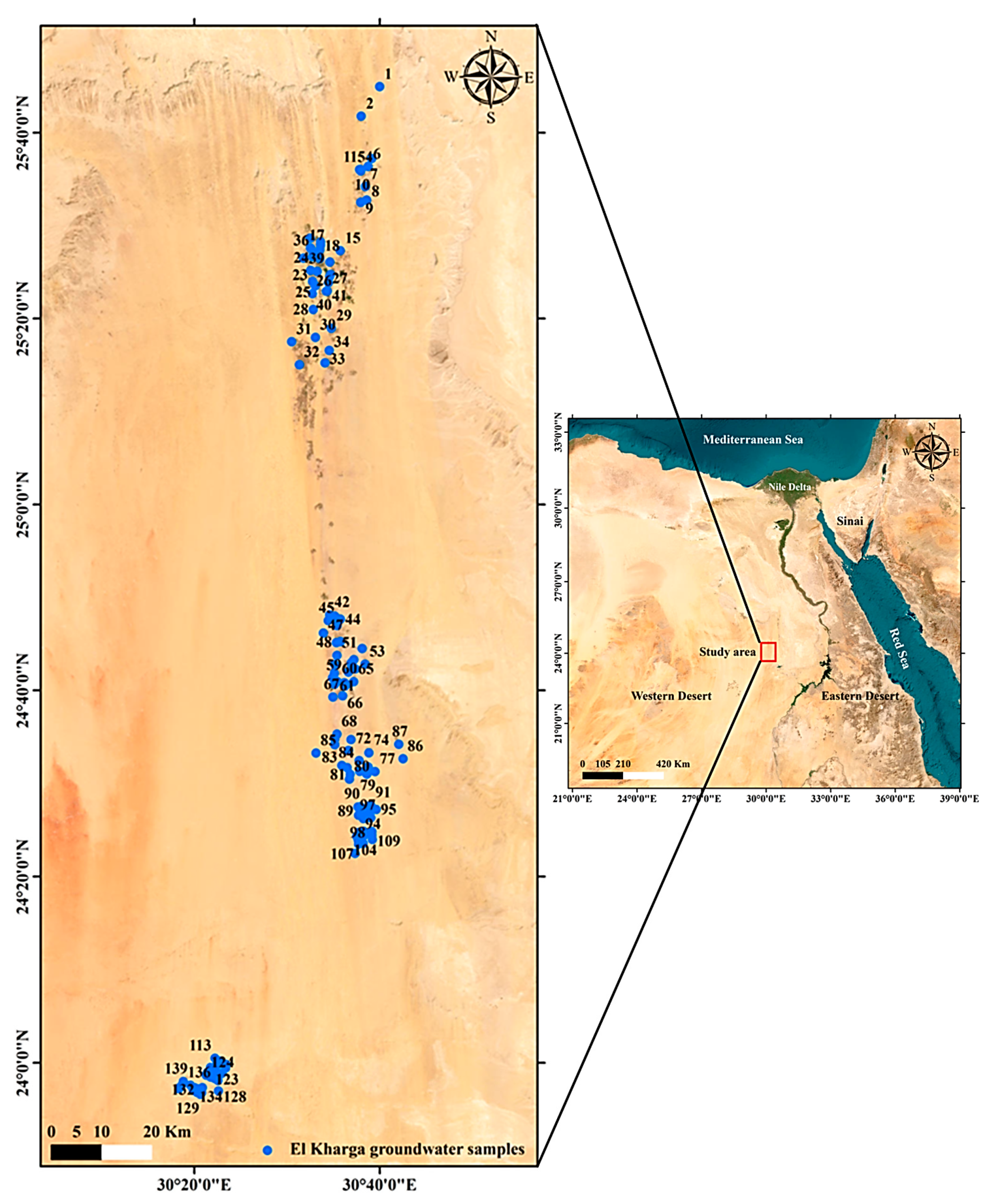
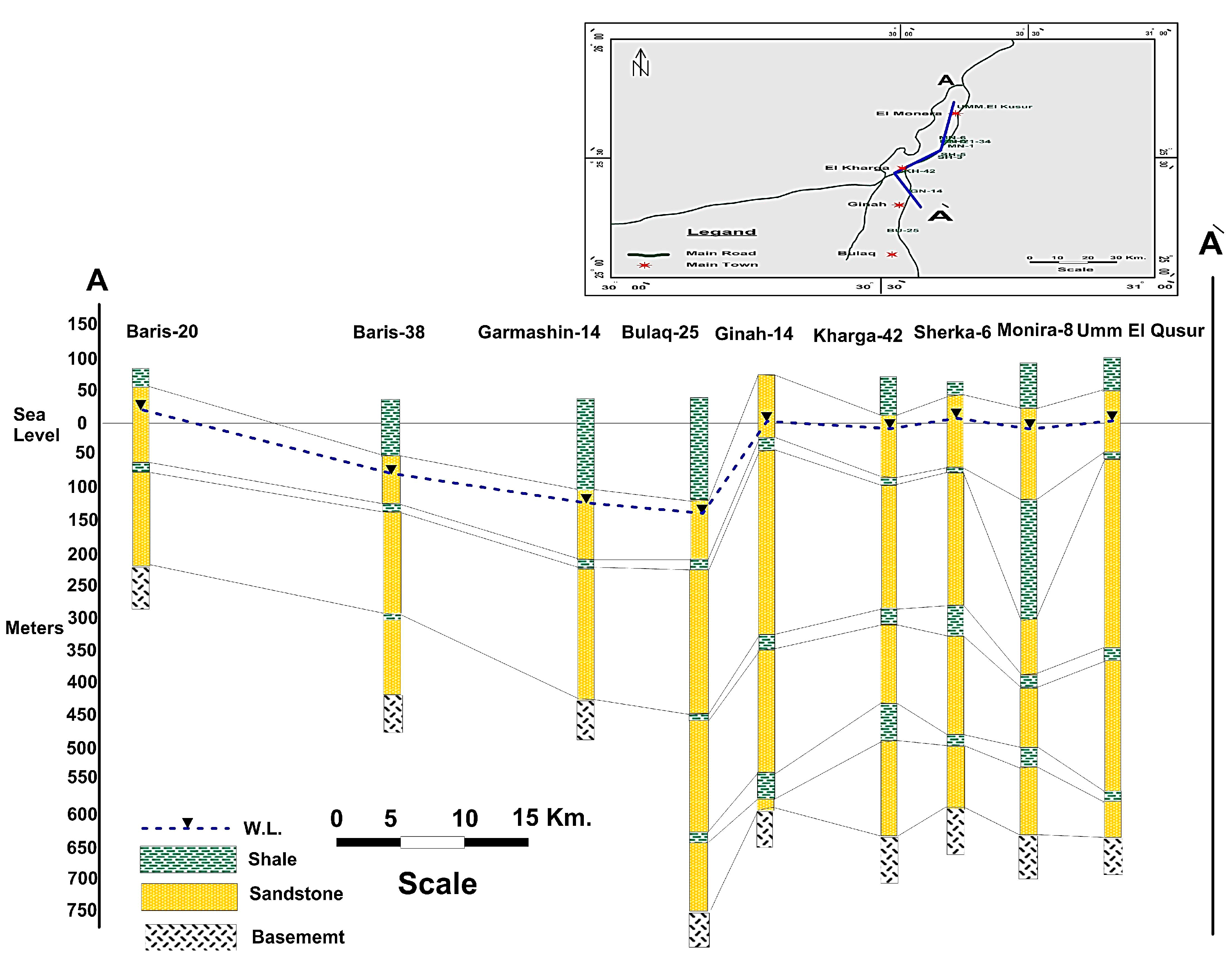
2.1. Site Description and Hydrogeological Settings
2.2. Sampling and Analysis
2.3. Indexing Approach
2.3.1. Irrigation Water Quality Indices (IWQIs)
2.3.2. Irrigation Water Quality Index (IWQI)
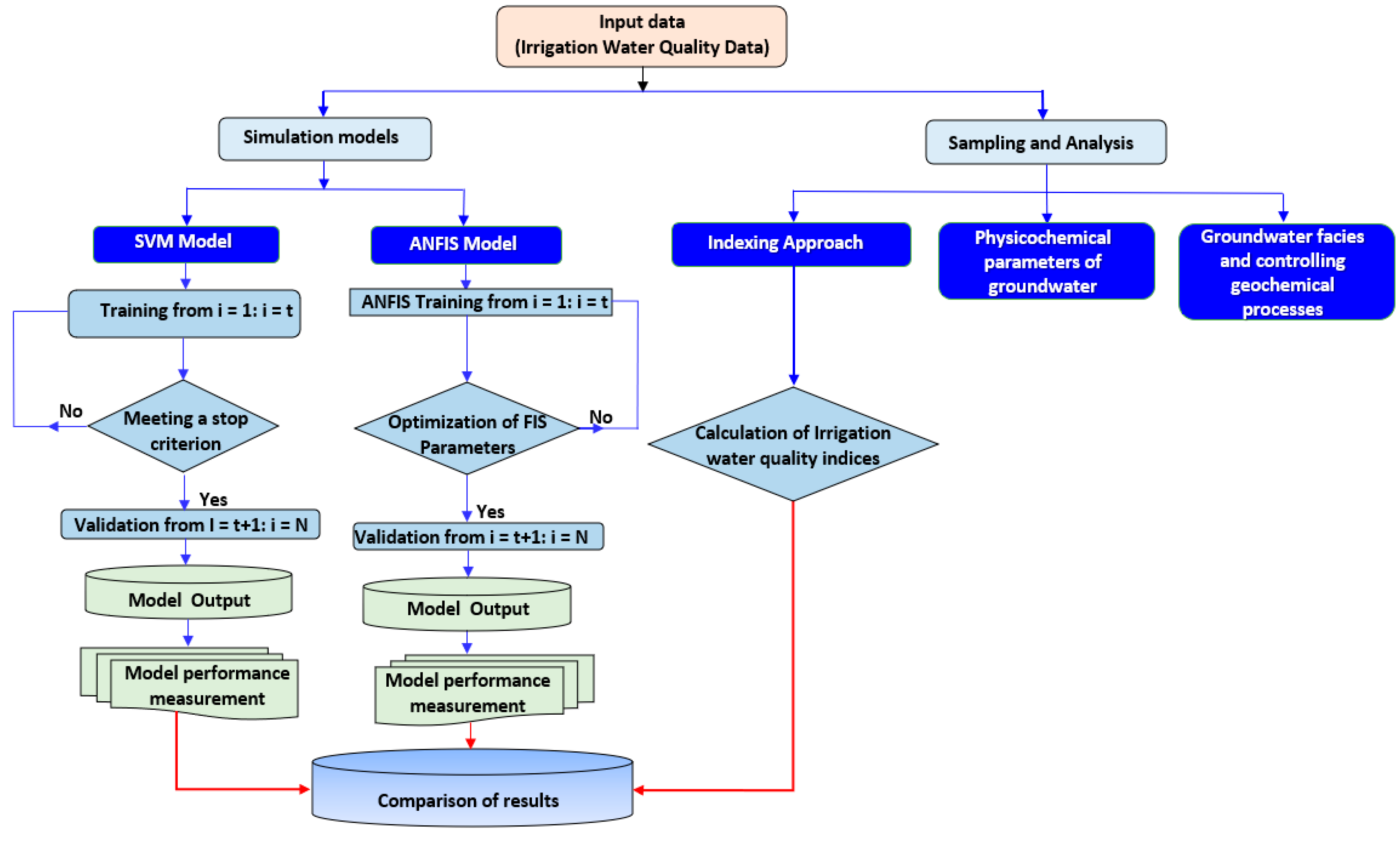
2.4. Simulation Models
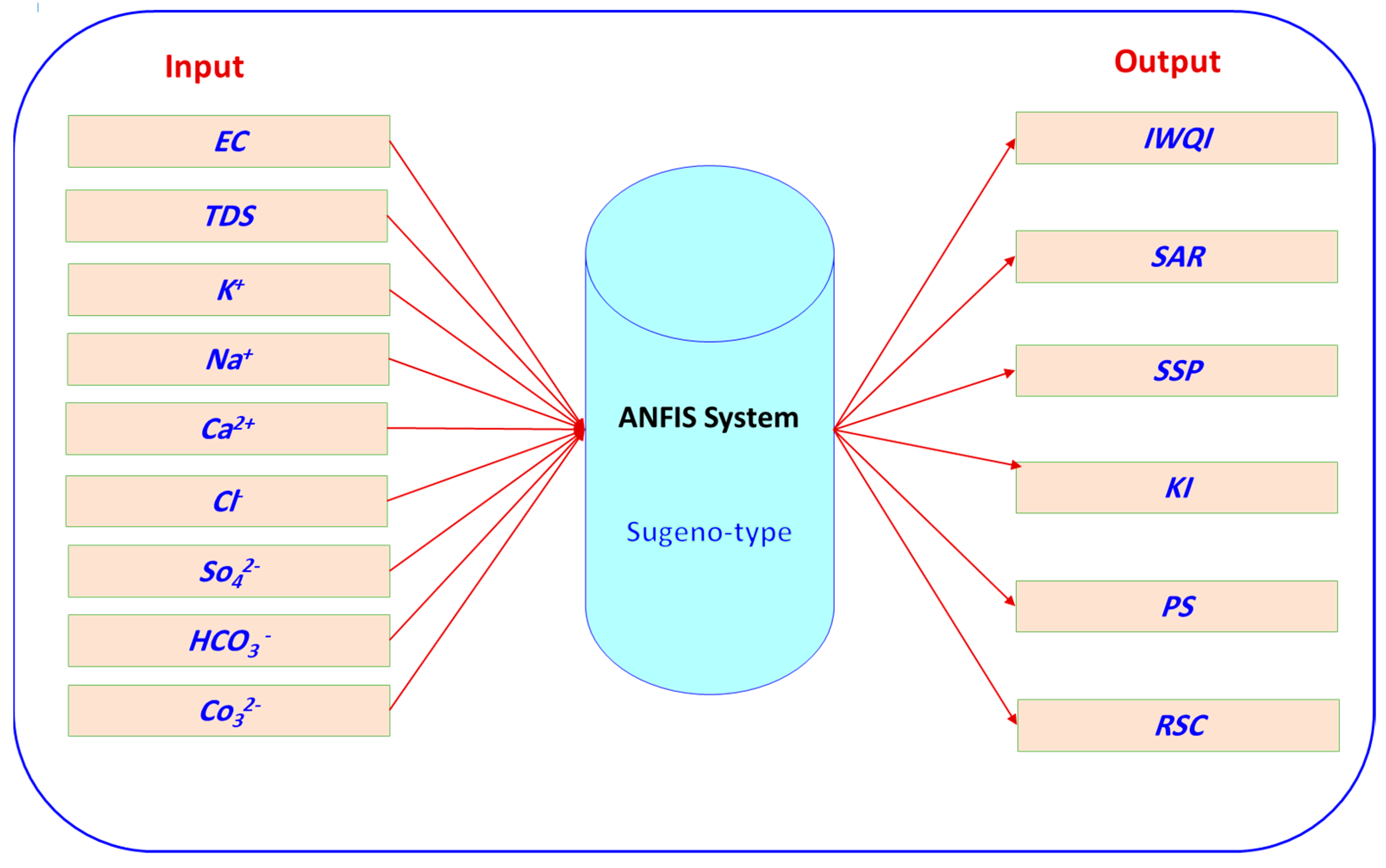
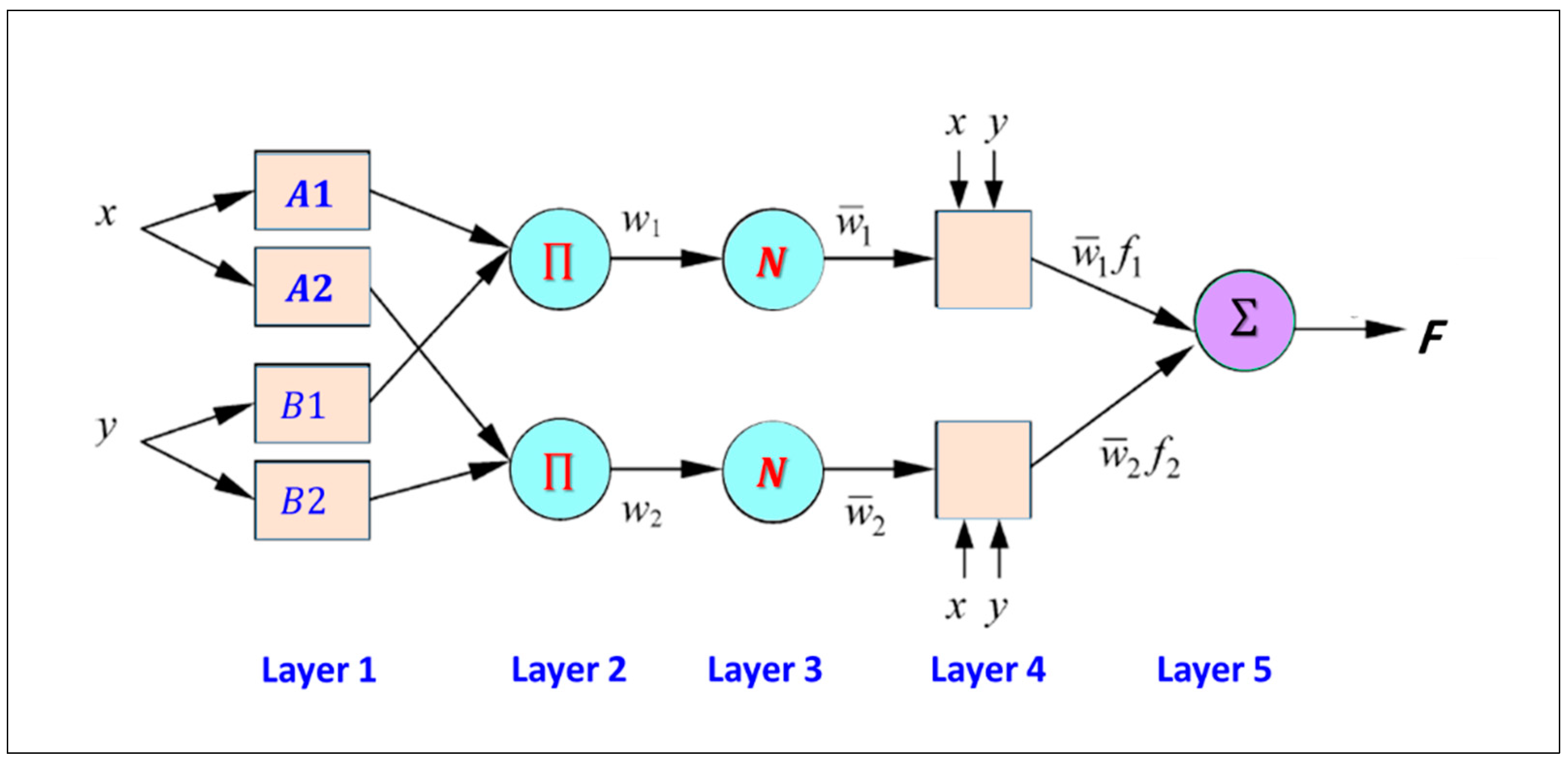
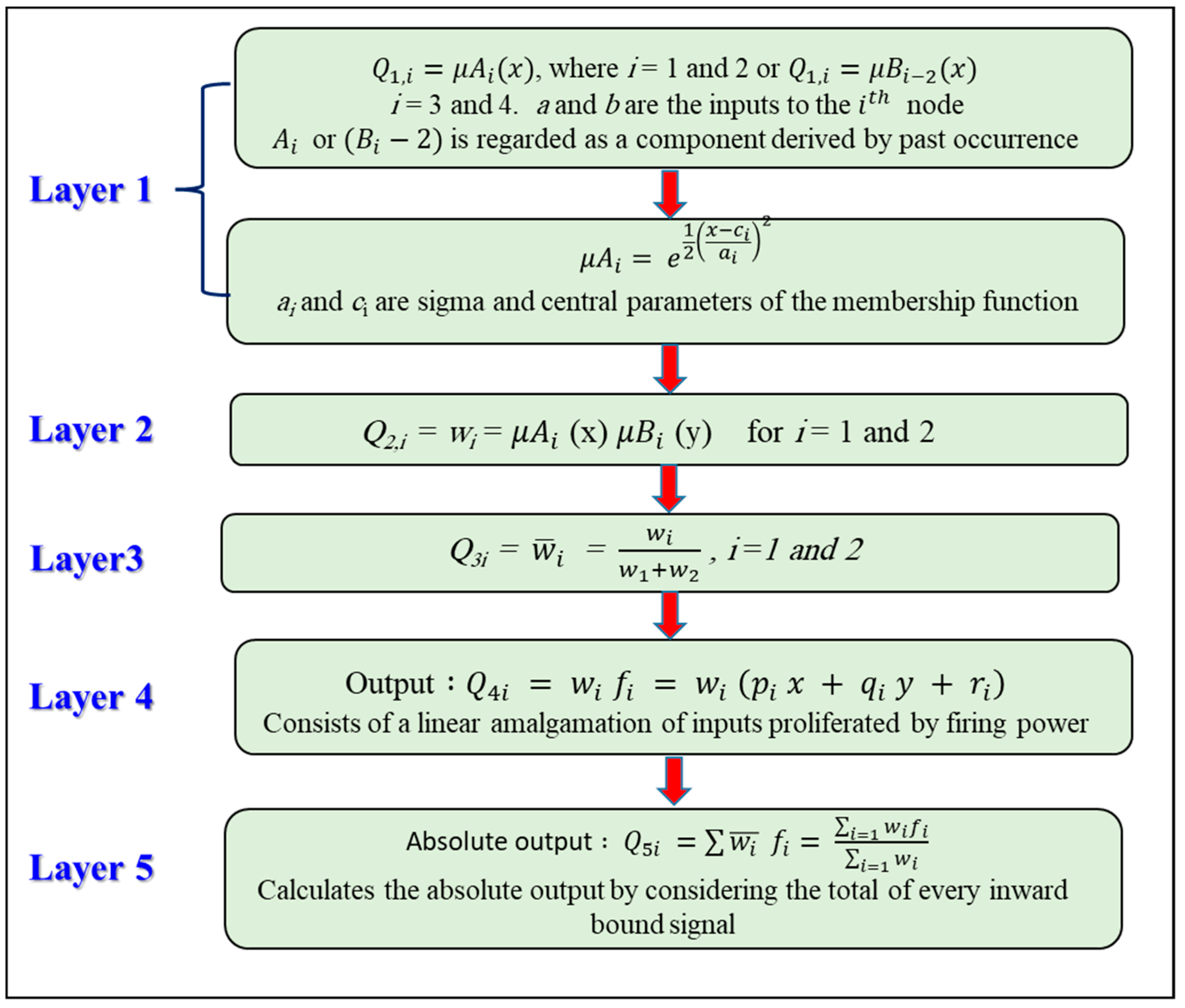
2.5. Adaptive Neuro-Fuzzy Inference System
2.6. Performance Evaluation of the Simulation Models
- (a)
- Nash–Sutcliffe efficiency coefficient (NSE):
- (b)
- The mean absolute error (MAD):
- (c)
- The absolute variance fraction, R2:
- (d)
- The root mean square error (RMSE):
3. Results and Discussions
3.1. Physicochemical Parameters of the Groundwater
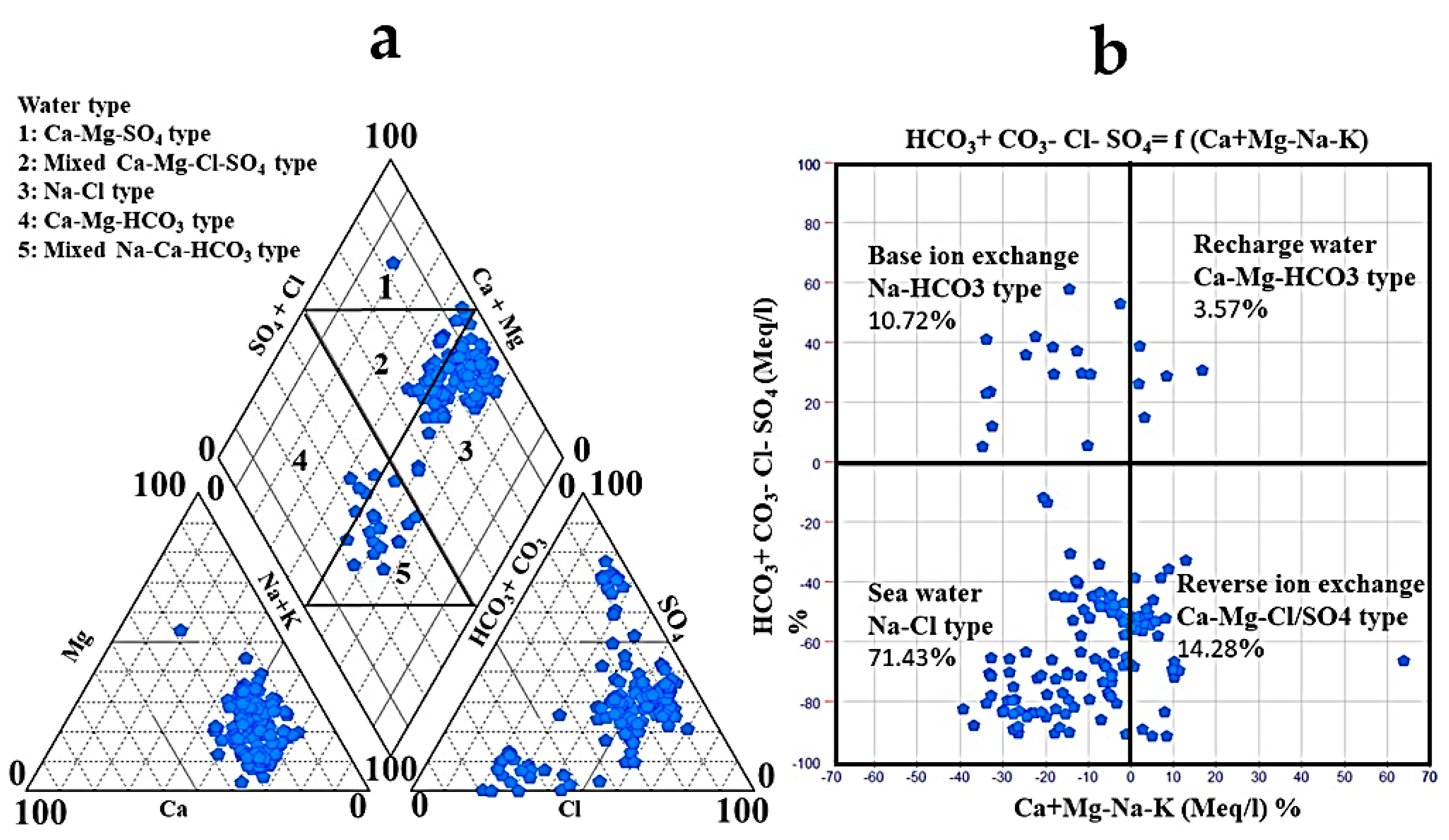
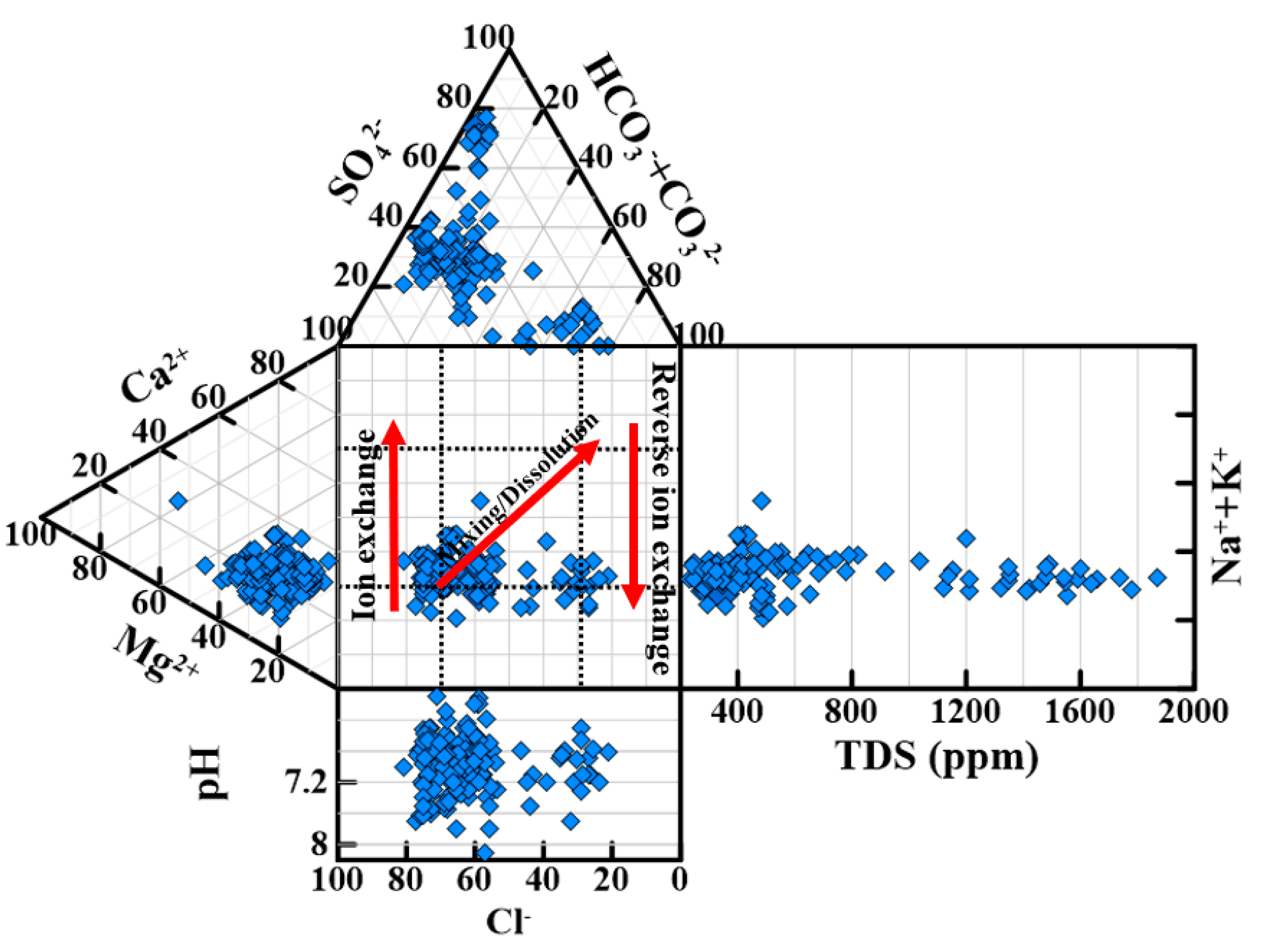
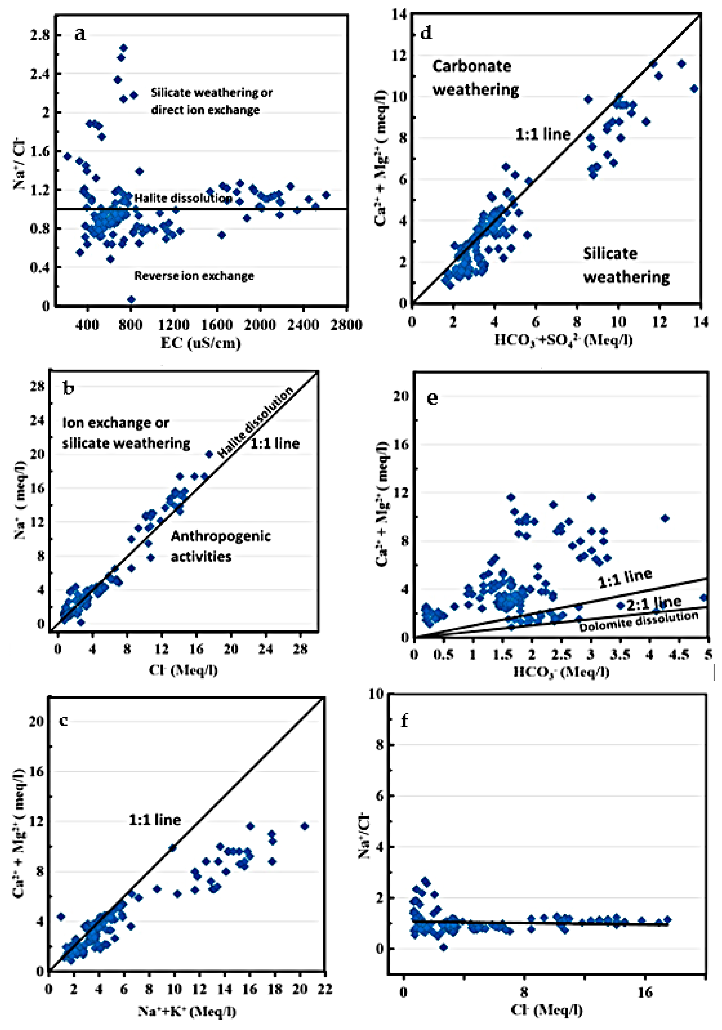
3.2. Groundwater Facies and Controlling Geochemical Processes
3.3. Water Quality Indices for Agricultural Purposes
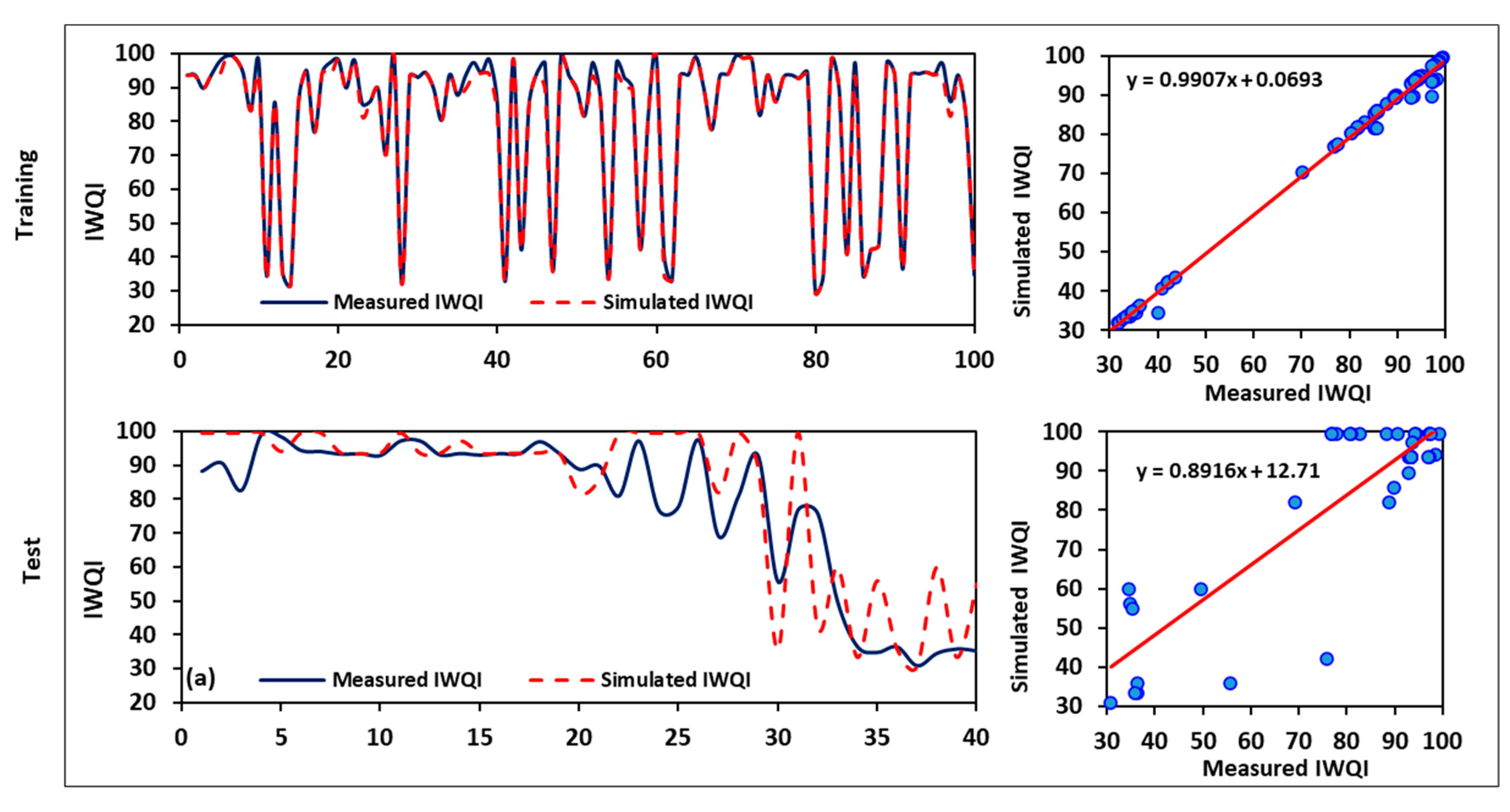
3.3.1. Irrigation Water Quality Index (IWQI)
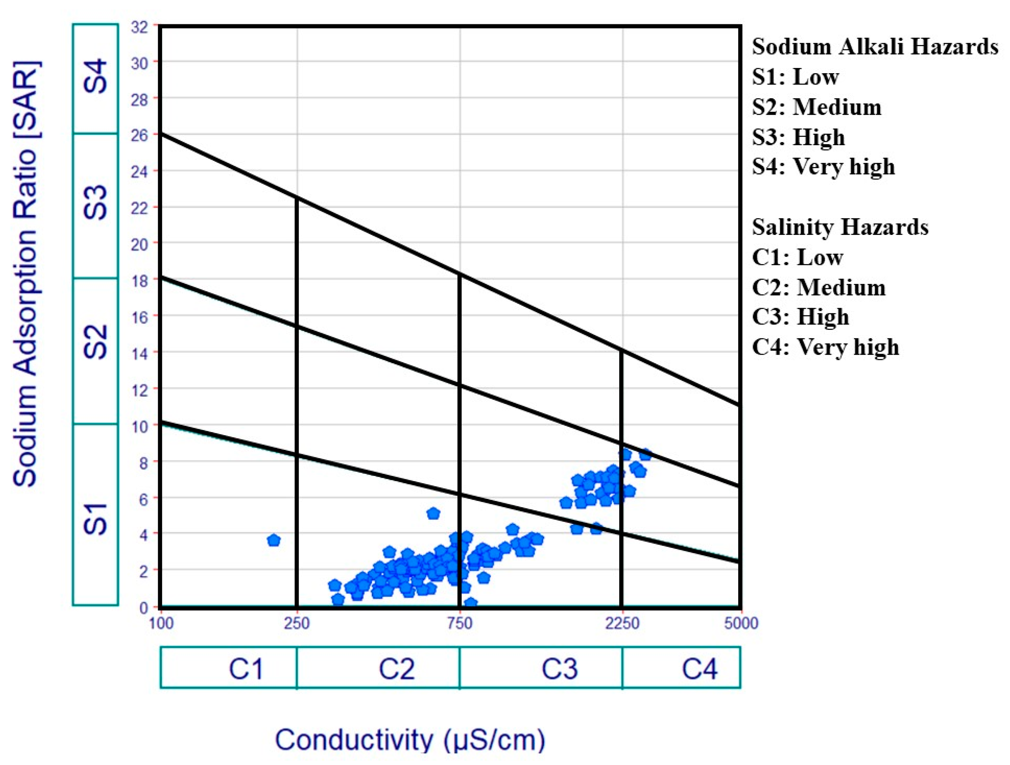
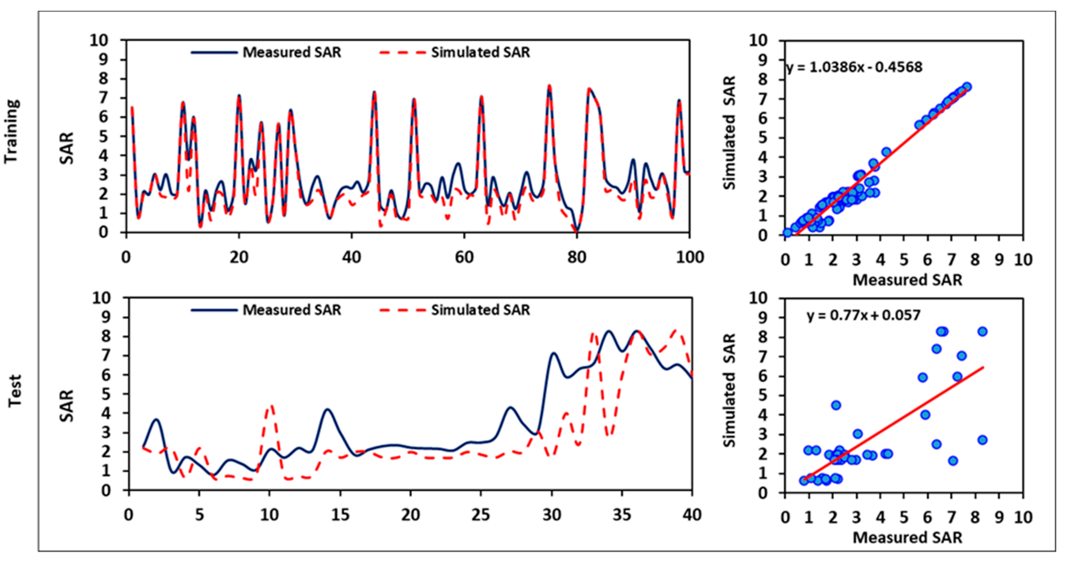
3.3.2. Sodium Adsorption Ratio (SAR)
3.3.3. Soluble Sodium Percentage (SSP)
3.3.4. Potential Salinity (PS)
3.3.5. Kelley Index (KI)
3.3.6. Residual Sodium Carbonate (RSC)
3.4. Simulation of Models
3.4.1. SVM Model
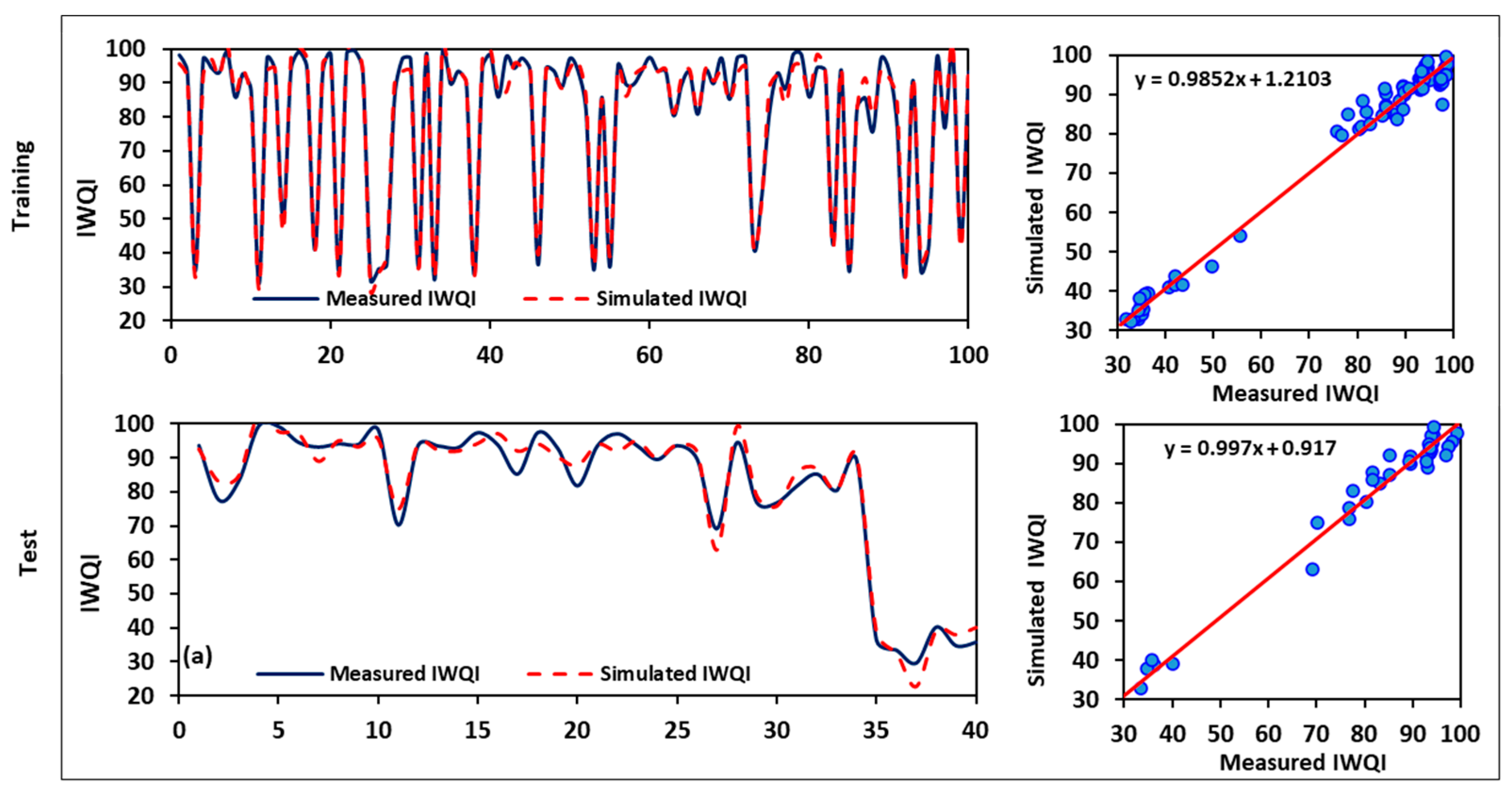
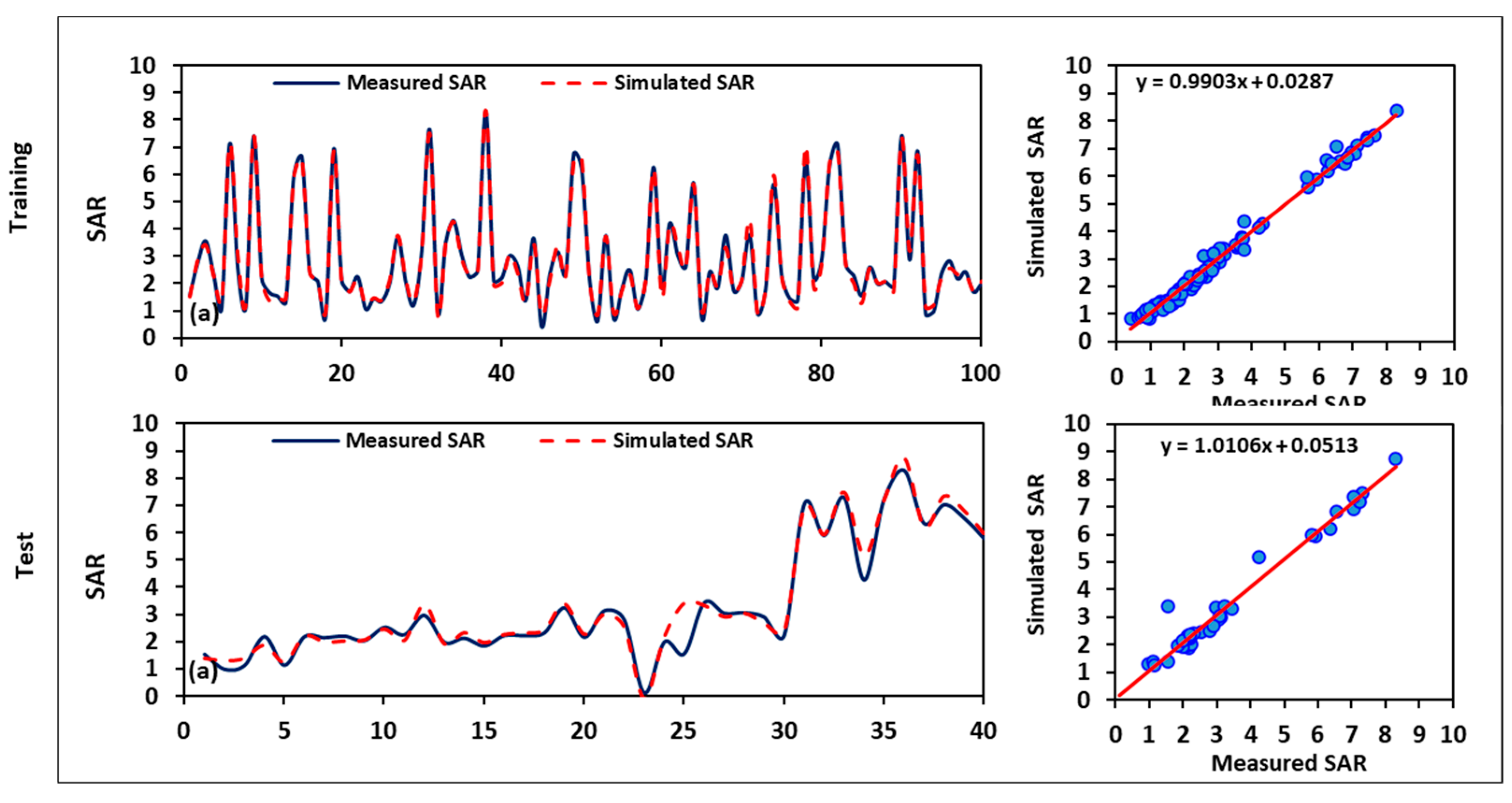
3.4.2. ANFIS Model
3.4.3. Theoretical and Practical Implications
4. Conclusions
Supplementary Materials
Author Contributions
Funding
Institutional Review Board Statement
Informed Consent Statement
Data Availability Statement
Conflicts of Interest
References
- El-Rawy, M.; De Smedt, F. Estimation and Mapping of the Transmissivity of the Nubian Sandstone Aquifer in the Kharga Oasis, Egypt. Water 2020, 12, 604. [Google Scholar] [CrossRef]
- Heinl, M.; Thorweihe, U.; Meisner, B.; Wycisk, P. Geopotential and Ecology–Analysis of a Desert Region; Schweizerbart Science Publishers: Stuttgart, Germany, 1993. [Google Scholar]
- Mahmod, W.E.; Watanabe, K. Modified Grey Model and Its Application to Groundwater Flow Analysis with Limited Hydrogeological Data: A Case Study of the Nubian Sandstone, Kharga Oasis, Egypt. Environ. Monit. Assess. 2014, 186, 1063–1081. [Google Scholar] [CrossRef] [PubMed]
- Ebraheem, A.; Riad, S.; Wycisk, P.; Seif El-Nasr, A. Simulation of Impact of Present and Future Groundwater Extraction from the Non-Replenished Nubian Sandstone Aquifer in Southwest Egypt. Environ. Geol. 2002, 43, 188–196. [Google Scholar]
- Mahmod, W.E.; Watanabe, K.; Zahr-Eldeen, A.A. Analysis of Groundwater Flow in Arid Areas with Limited Hydrogeological Data Using the Grey Model: A Case Study of the Nubian Sandstone, Kharga Oasis, Egypt. Hydrogeol. J. 2013, 21, 1021–1034. [Google Scholar] [CrossRef]
- Gaagai, A.; Aouissi, H.A.; Bencedira, S.; Hinge, G.; Athamena, A.; Haddam, S.; Gad, M.; Elsherbiny, O.; Elsayed, S.; Eid, M.H.; et al. Application of Water Quality Indices, Machine Learning Approaches, and GIS to Identify Groundwater Quality for Irrigation Purposes: A Case Study of Sahara Aquifer, Doucen Plain, Algeria. Water 2023, 15, 289. [Google Scholar] [CrossRef]
- Singh, S.; Ghosh, N.C.; Gurjar, S.; Krishan, G.; Kumar, S.; Berwal, P. Index-Based Assessment of Suitability of Water Quality for Irrigation Purpose under Indian Conditions. Environ. Monit. Assess. 2018, 190, 29. [Google Scholar] [CrossRef]
- Wu, J.; Li, P.; Qian, H. Hydrochemical Characterization of Drinking Groundwater with Special Reference to Fluoride in an Arid Area of China and the Control of Aquifer Leakage on Its Concentrations. Environ. Earth Sci. 2015, 73, 8575–8588. [Google Scholar] [CrossRef]
- Venkateswaran, S.; Ayyandurai, R. Groundwater Characterization and Quality Assesment for Irrigational Purpose Using Gis-A Case Study of Kadavanar Watershed Tamilnadu, India. J. Appl. Geochem. 2015, 17, 488–496. [Google Scholar]
- Sridharan, M.; Senthil Nathan, D. Groundwater Quality Assessment for Domestic and Agriculture Purposes in Puducherry Region. Appl. Water Sci. 2017, 7, 4037–4053. [Google Scholar] [CrossRef]
- Khan, A.F.; Srinivasamoorthy, K.; Rabina, C. Hydrochemical Characteristics and Quality Assessment of Groundwater along the Coastal Tracts of Tamil Nadu and Puducherry, India. Appl. Water. Sci. 2020, 10, 74. [Google Scholar] [CrossRef]
- Duan, L.; Wang, B.; Heck, K.; Guo, S.; Clark, C.A.; Arredondo, J.; Wang, M.; Senftle, T.P.; Westerhoff, P.; Wen, X.; et al. Efficient Photocatalytic PFOA Degradation over Boron Nitride. Environ. Sci. Technol. Lett. 2020, 7, 613–619. [Google Scholar] [CrossRef]
- Elsayed, S.; Ibrahim, H.; Hussein, H.; Elsherbiny, O.; Elmetwalli, A.H.; Moghanm, F.S.; Ghoneim, A.M.; Danish, S.; Datta, R.; Gad, M. Assessment of Water Quality in Lake Qaroun Using Ground-Based Remote Sensing Data and Artificial Neural Networks. Water 2021, 13, 3094. [Google Scholar] [CrossRef]
- Khadr, M.; Gad, M.; El-Hendawy, S.; Al-Suhaibani, N.; Dewir, Y.H.; Tahir, M.U.; Mubushar, M.; Elsayed, S. The Integration of Multivariate Statistical Approaches, Hyperspectral Reflectance, and Data-Driven Modeling for Assessing the Quality and Suitability of Groundwater for Irrigation. Water 2020, 13, 35. [Google Scholar] [CrossRef]
- Gad, M.; Dahab, K.; Ibrahim, H. Applying of a Geochemical Model on the Nubian Sandstone Aquifer in Siwa Oasis, Western Desert, Egypt. Environ. Earth Sci. 2018, 77, 401. [Google Scholar] [CrossRef]
- Abraham, B.G.; Nata, T.; Elias, J. Application of Water Quality Index to Assess Suitablity of Groundwater Quality for Drinking Purposes in Hantebet Watershed, Tigray, Northern Ethiopia. ISABB J. Food Agric. Sci. 2011, 1, 22–30. [Google Scholar]
- Rajankar, P.N.; Tambekar, D.H.; Wate, S.R. Groundwater Quality and Water Quality Index at Bhandara District. Environ. Monit. Assess. 2011, 179, 619–625. [Google Scholar] [CrossRef] [PubMed]
- Ravikumar, P.; Aneesul Mehmood, M.; Somashekar, R.K. Water Quality Index to Determine the Surface Water Quality of Sankey Tank and Mallathahalli Lake, Bangalore Urban District, Karnataka, India. Appl. Water Sci. 2013, 3, 247–261. [Google Scholar] [CrossRef]
- Ocampo-Duque, W.; Osorio, C.; Piamba, C.; Schuhmacher, M.; Domingo, J.L. Water Quality Analysis in Rivers with Non-Parametric Probability Distributions and Fuzzy Inference Systems: Application to the Cauca River, Colombia. Environ. Int. 2013, 52, 17–28. [Google Scholar] [CrossRef]
- Sutadian, A.D.; Muttil, N.; Yilmaz, A.G.; Perera, B.J.C. Development of River Water Quality Indices—A Review. Environ. Monit. Assess. 2016, 188, 58. [Google Scholar] [CrossRef]
- Masoud, M.; El Osta, M.; Alqarawy, A.; Elsayed, S.; Gad, M. Evaluation of Groundwater Quality for Agricultural under Different Conditions Using Water Quality Indices, Partial Least Squares Regression Models, and GIS Approaches. Appl. Water Sci. 2022, 12, 244. [Google Scholar] [CrossRef]
- El Osta, M.; Masoud, M.; Alqarawy, A.; Elsayed, S.; Gad, M. Groundwater Suitability for Drinking and Irrigation Using Water Quality Indices and Multivariate Modeling in Makkah Al-Mukarramah Province, Saudi Arabia. Water 2022, 14, 483. [Google Scholar] [CrossRef]
- Ayers, R.; Westcott, D. Water Quality for Agriculture. FAO Irrigation and Drainage Paper 29 Rev. 1; Food and Agricultural Organisation of the United Nations: Rome, Italy, 1994. [Google Scholar]
- Srinivasamoorthy, K.; Gopinath, M.; Chidambaram, S.; Vasanthavigar, M.; Sarma, V.S. Hydrochemical Characterization and Quality Appraisal of Groundwater from Pungar Sub Basin, Tamilnadu, India. J. King Saud Univ.-Sci. 2014, 26, 37–52. [Google Scholar] [CrossRef]
- Gopinath, S.; Srinivasamoorthy, K.; Saravanan, K.; Prakash, R.; Suma, C.S.; Khan, F.; Senthilnathan, D.; Sarma, V.S.; Devi, P. Hydrogeochemical Characteristics of Coastal Groundwater in Nagapattinam and Karaikal Aquifers: Implications for Saline Intrusion and Agricultural Suitability. J. Coast. Sci. 2015, 2, 1–11. [Google Scholar]
- Aravinthasamy, P.; Karunanidhi, D.; Subba Rao, N.; Subramani, T.; Srinivasamoorthy, K. Irrigation Risk Assessment of Groundwater in a Non-Perennial River Basin of South India: Implication from Irrigation Water Quality Index (IWQI) and Geographical Information System (GIS) Approaches. Arab. J. Geosci. 2020, 13, 1125. [Google Scholar] [CrossRef]
- Ahmed, M.T.; Hasan, M.Y.; Monir, M.U.; Samad, M.A.; Rahman, M.M.; Islam Rifat, M.S.; Islam, M.N.; Khan, A.A.S.; Biswas, P.K.; Jamil, A.H.M.N. Evaluation of Hydrochemical Properties and Groundwater Suitability for Irrigation Uses in Southwestern Zones of Jashore, Bangladesh. Groundw. Sustain. Dev. 2020, 11, 100441. [Google Scholar] [CrossRef]
- Bhunia, G.S.; Keshavarzi, A.; Shit, P.K.; Omran, E.-S.E.; Bagherzadeh, A. Evaluation of Groundwater Quality and Its Suitability for Drinking and Irrigation Using GIS and Geostatistics Techniques in Semiarid Region of Neyshabur, Iran. Appl. Water Sci. 2018, 8, 168. [Google Scholar] [CrossRef]
- Thapa, R.; Gupta, S.; Reddy, D.V.; Kaur, H. An Evaluation of Irrigation Water Suitability in the Dwarka River Basin through the Use of GIS-Based Modelling. Environ. Earth Sci. 2017, 76, 471. [Google Scholar] [CrossRef]
- Alqarawy, A.; El Osta, M.; Masoud, M.; Elsayed, S.; Gad, M. Use of Hyperspectral Reflectance and Water Quality Indices to Assess Groundwater Quality for Drinking in Arid Regions, Saudi Arabia. Water 2022, 14, 2311. [Google Scholar] [CrossRef]
- Gad, M.; Abou El-Safa, M.M.; Farouk, M.; Hussein, H.; Alnemari, A.M.; Elsayed, S.; Khalifa, M.M.; Moghanm, F.S.; Eid, E.M.; Saleh, A.H. Integration of Water Quality Indices and Multivariate Modeling for Assessing Surface Water Quality in Qaroun Lake, Egypt. Water 2021, 13, 2258. [Google Scholar] [CrossRef]
- Gad, M.; Saleh, A.H.; Hussein, H.; Farouk, M.; Elsayed, S. Appraisal of Surface Water Quality of Nile River Using Water Quality Indices, Spectral Signature and Multivariate Modeling. Water 2022, 14, 1131. [Google Scholar] [CrossRef]
- Elsayed, S.; Hussein, H.; Moghanm, F.S.; Khedher, K.M.; Eid, E.M.; Gad, M. Application of Irrigation Water Quality Indices and Multivariate Statistical Techniques for Surface Water Quality Assessments in the Northern Nile Delta, Egypt. Water 2020, 12, 3300. [Google Scholar] [CrossRef]
- Wong, Y.J.; Shimizu, Y.; Kamiya, A.; Maneechot, L.; Bharambe, K.P.; Fong, C.S.; Nik Sulaiman, N.M. Application of Artificial Intelligence Methods for Monsoonal River Classification in Selangor River Basin, Malaysia. Environ. Monit. Assess. 2021, 193, 438. [Google Scholar] [CrossRef]
- Wong, Y.J.; Shimizu, Y.; He, K.; Nik Sulaiman, N.M. Comparison among Different ASEAN Water Quality Indices for the Assessment of the Spatial Variation of Surface Water Quality in the Selangor River Basin, Malaysia. Environ. Monit. Assess. 2020, 192, 644. [Google Scholar] [CrossRef] [PubMed]
- Eid, M.H.; Elbagory, M.; Tamma, A.A.; Gad, M.; Elsayed, S.; Hussein, H.; Moghanm, F.S.; Omara, A.E.-D.; Kovács, A.; Péter, S. Evaluation of Groundwater Quality for Irrigation in Deep Aquifers Using Multiple Graphical and Indexing Approaches Supported with Machine Learning Models and GIS Techniques, Souf Valley, Algeria. Water 2023, 15, 182. [Google Scholar] [CrossRef]
- Tao, H.; Hameed, M.M.; Marhoon, H.A.; Zounemat-Kermani, M.; Salim, H.; Sungwon, K.; Sulaiman, S.O.; Tan, M.L.; Sa’adi, Z.; Mehr, A.D.; et al. Groundwater level prediction using machine learning models: A comprehensive review. Neurocomputing 2022, 489, 271–308. [Google Scholar] [CrossRef]
- Rode, M.; Arhonditsis, G.; Balin, D.; Kebede, T.; Krysanova, V.; van Griensven, A.; van der Zee, S.E.A.T.M. New Challenges in Integrated Water Quality Modelling. Hydrol. Process. 2010, 24, 3447–3461. [Google Scholar] [CrossRef]
- Khadr, M.; Elshemy, M. Data-Driven Modeling for Water Quality Prediction Case Study: The Drains System Associated with Manzala Lake, Egypt. Ain Shams Eng. J. 2017, 8, 549–557. [Google Scholar] [CrossRef]
- Wang, Z.-Y.; Qiu, J.; Li, F.-F. Hybrid Models Combining EMD/EEMD and ARIMA for Long-Term Streamflow Forecasting. Water 2018, 10, 853. [Google Scholar] [CrossRef]
- Zhou, J.; Peng, T.; Zhang, C.; Sun, N. Data Pre-Analysis and Ensemble of Various Artificial Neural Networks for Monthly Streamflow Forecasting. Water 2018, 10, 628. [Google Scholar] [CrossRef]
- Noori, R.; Karbassi, A.R.; Mehdizadeh, H.; Vesali-Naseh, M.; Sabahi, M.S. A Framework Development for Predicting the Longitudinal Dispersion Coefficient in Natural Streams Using an Artificial Neural Network. Environ. Prog. Sustain. Energy 2011, 30, 439–449. [Google Scholar] [CrossRef]
- Sherif, M.I.; Sturchio, N.C. Elevated Radium Levels in Nubian Aquifer Groundwater of Northeastern Africa. Sci. Rep. 2021, 11, 78. [Google Scholar] [CrossRef]
- Soliman, M.M. Land and Water Resources Assessment for Sustainable Agricultural Development in EL-kharga Oases by Using Remote Sensing and Geographic Information System. Menoufia J. Soil Sci. 2020, 5, 55–83. [Google Scholar] [CrossRef]
- Assaad, F.A. Hydrogeological Aspects and Environmental Concerns of the New Valley Project, Western Desert, Egypt, with Special Emphasis on the Southern Area. Environ. Geol. Water Sci. 1988, 12, 141–161. [Google Scholar] [CrossRef]
- Kehl, H.; Bornkamm, R. Landscape Ecology and Vegetation Units of the Western Desert of Egypt. Catena Suppl. 1993, 155–178. Available online: http://geoprodig.cnrs.fr/items/show/85519 (accessed on 29 January 2023).
- Salman, A.B.; Howari, F.M.; El-Sankary, M.M.; Wali, A.M.; Saleh, M.M. Environmental Impact and Natural Hazards on Kharga Oasis Monumental Sites, Western Desert of Egypt. J. Afr. Earth Sci. 2010, 58, 341–353. [Google Scholar] [CrossRef]
- Lamoreaux, P.E.; Memon, B.A.; Idris, H. Groundwater Development, Kharga Oases, Western Desert of Egypt: A Long-Term Environmental Concern. Environ. Geol. Water Sci. 1985, 7, 129–149. [Google Scholar] [CrossRef]
- Zahran, M.A.; Willis, A.J. The Vegetation of Egypt; Springer Science & Business Media: Berlin, Germany, 2008; p. 2. [Google Scholar]
- Fathy, R.G.; El Nagaty, M.; Atef, A.; El Gammal, N. Contributions to the Hydrogeological and Hydrochemical Characteristics of Nubia Sandstone Aquifer in Darb Al-Arbeain, South Western Desert, Egypt. Al-Azhar Bull. Sci. 2002, 13, 69–100. [Google Scholar]
- Elewa, H.H.; Fathy, R.G.; Qaddah, A.A. The Contribution of Geographic Information Systems and Remote Sensing in Determining Priority Areas for Hydrogeological Development, Darb El-Arbain Area, Western Desert, Egypt. Hydrogeol. J. 2010, 18, 1157–1171. [Google Scholar] [CrossRef]
- El Osta, M.; Hussein, H.; Tomas, K. Numerical Simulation of Groundwater Flow and Vulnerability in Wadi El-Natrun Depression and Vicinities, West Nile Delta, Egypt. J. Geol. Soc. India 2018, 92, 235–247. [Google Scholar] [CrossRef]
- El Osta, M.; Masoud, M.; Ezzeldin, H. Assessment of the Geochemical Evolution of Groundwater Quality near the El Kharga Oasis, Egypt Using NETPATH and Water Quality Indices. Environ. Earth Sci. 2020, 79, 56. [Google Scholar] [CrossRef]
- El Saeed, G.H.; Abdelmageed, N.B.; Riad, P.; Komy, M. Confined Aquifer Piezometric Head Depletion in the Dynamic State. JOKULL J. 2019, 69, 56–67. [Google Scholar]
- Domenico, P.A.; Schwartz, F.W. Physical and Chemical Hydrogeology; Wiley: New York, NY, USA, 1998; Volume 506. [Google Scholar]
- Richards, L.A. Diagnosis and Improvement of Saline and Alkali Soils; LWW: Philadelphia, PA, USA, 1954; p. 78. [Google Scholar]
- Kelley, W.P. Permissible Composition and Concentration of Irrigation Water. In Proceedings of the American Society of Civil Engineers 1940. Volume 66, pp. 607–613. Available online: https://www.scirp.org/(S(351jmbntvnsjt1aadkposzje))/reference/ReferencesPapers.aspx?ReferenceID=1927054 (accessed on 20 December 2022).
- Doneen, L.D. Water Quality for Agriculture; Department of Irrigation, University of California: Davis, CA, USA, 1964; p. 48. [Google Scholar]
- Eaton, F.M. Significance of Carbonates in Irrigation Waters. Soil Sci. 1950, 69, 123–134. [Google Scholar] [CrossRef]
- Meireles, A.C.M.; Andrade, E.M.D.; Chaves, L.C.G.; Frischkorn, H.; Crisostomo, L.A. A New Proposal of the Classification of Irrigation Water. Rev. Ciênc. Agron. 2010, 41, 349–357. [Google Scholar] [CrossRef]
- Abbasnia, A.; Yousefi, N.; Mahvi, A.H.; Nabizadeh, R.; Radfard, M.; Yousefi, M.; Alimohammadi, M. Evaluation of Groundwater Quality Using Water Quality Index and Its Suitability for Assessing Water for Drinking and Irrigation Purposes: Case Study of Sistan and Baluchistan Province (Iran). Hum. Ecol. Risk Assess. Int. J. 2019, 25, 988–1005. [Google Scholar] [CrossRef]
- Müller, K.-R.; Smola, A.J.; Rätsch, G.; Schölkopf, B.; Kohlmorgen, J.; Vapnik, V. Predicting Time Series with Support Vector Machines. In Artificial Neural Networks—ICANN’97; Gerstner, W., Germond, A., Hasler, M., Nicoud, J.-D., Eds.; Lecture Notes in Computer Science; Springer: Berlin/Heidelberg, Germany, 1997; Volume 1327, pp. 999–1004. [Google Scholar]
- Khadr, M. Water Resources Management in the Context of Drought (an Application to the Ruhr River Basin in Germany); Shaker: Düren, Germany, 2011. [Google Scholar]
- Freeze, R.A.; Cherry, J. Groundwater; Prenctice Hall. Inc.: Hoboken, NJ, USA, 1979. [Google Scholar]
- Piper, A.M. A Graphic Procedure in the Geochemical Interpretation of Water-Analyses. Trans. AGU 1944, 25, 914. [Google Scholar] [CrossRef]
- Chadha, D.K. A Proposed New Diagram for Geochemical Classification of Natural Waters and Interpretation of Chemical Data. Hydrogeol. J. 1999, 7, 431–439. [Google Scholar] [CrossRef]
- Antonakos, A.; Lambrakis, N. Hydrodynamic Characteristics and Nitrate Propagation in Sparta Aquifer. Water Res. 2000, 34, 3977–3986. [Google Scholar] [CrossRef]
- Elango, L.; Kannan, R. Chapter 11 Rock–Water Interaction and Its Control on Chemical Composition of Groundwater. In Dev. Environ. Sci. 2007, 5, 229–243. [Google Scholar]
- Jalali, M. Salinization of Groundwater in Arid and Semi-Arid Zones: An Example from Tajarak, Western Iran. Environ. Geol. 2007, 52, 1133–1149. [Google Scholar] [CrossRef]
- Srinivasamoorthy, K.; Chidambaram, S.; Prasanna, M.V.; Vasanthavihar, M.; Peter, J.; Anandhan, P. Identification of Major Sources Controlling Groundwater Chemistry from a Hard Rock Terrain—A Case Study from Mettur Taluk, Salem District, Tamil Nadu, India. J. Earth Syst. Sci. 2008, 117, 49–58. [Google Scholar] [CrossRef]
- Jacks, G.; Sefe, F.; Carling, M.; Hammar, M.; Letsamao, P. Tentative Nitrogen Budget for Pit Latrines-Eastern Botswana. Environ. Geol. 1999, 38, 199–203. [Google Scholar] [CrossRef]
- Fisher, R.S.; Mullican, W.F., III. Hydrochemical Evolution of Sodium-Sulfate and Sodium-Chloride Groundwater Beneath the Northern Chihuahuan Desert, Trans-Pecos, Texas, USA. Hydrogeol. J. 1997, 5, 4–16. [Google Scholar] [CrossRef]
- Meybeck, M. Global Chemical Weathering of Surficial Rocks Estimated from River Dissolved Loads. Am. J. Sci. 1987, 287, 401–428. [Google Scholar] [CrossRef]
- Jankowski, J.; Acworth, R.I. Impact of Debris-Flow Deposits on Hydrogeochemical Processes and the Developement of Dryland Salinity in the Yass River Catchment, New South Wales, Australia. Hydrogeol. J. 1997, 5, 71–88. [Google Scholar] [CrossRef]
- Rajmohan, N.; Elango, L. Identification and Evolution of Hydrogeochemical Processes in the Groundwater Environment in an Area of the Palar and Cheyyar River Basins, Southern India. Environ. Geol. 2004, 46, 47–61. [Google Scholar] [CrossRef]
- Sami, K. Recharge Mechanisms and Geochemical Processes in a Semi-Arid Sedimentary Basin, Eastern Cape, South Africa. J. Hydrol. 1992, 139, 27–48. [Google Scholar] [CrossRef]
- Spears, D.A. Mineralogical Control of the Chemical Evolution of Groundwater. Solute Process. 1986, 512. [Google Scholar]
- Nazzal, Y.; Ahmed, I.; Al-Arifi, N.S.N.; Ghrefat, H.; Zaidi, F.K.; El-Waheidi, M.M.; Batayneh, A.; Zumlot, T. A Pragmatic Approach to Study the Groundwater Quality Suitability for Domestic and Agricultural Usage, Saq Aquifer, Northwest of Saudi Arabia. Environ. Monit. Assess. 2014, 186, 4655–4667. [Google Scholar] [CrossRef]
- Gad, M.; El-Hendawy, S.; Al-Suhaibani, N.; Tahir, M.U.; Mubushar, M.; Elsayed, S. Combining Hydrogeochemical Characterization and a Hyperspectral Reflectance Tool for Assessing Quality and Suitability of Two Groundwater Resources for Irrigation in Egypt. Water 2020, 12, 2169. [Google Scholar] [CrossRef]
- Kaka, E.A.; Akiti, T.T.; Nartey, V.K.; Bam, E.K.P.; Adomako, D. Hydrochemistry and Evaluation of Groundwater Suitability for Irrigation and Drinking Purposes in the Southeastern Volta River Basin: Manyakrobo Area, Ghana. Elixir Agric. 2011, 39, 4793–4807. [Google Scholar]
- Kawo, N.S.; Karuppannan, S. Groundwater Quality Assessment Using Water Quality Index and GIS Technique in Modjo River Basin, Central Ethiopia. J. Afr. Earth Sci. 2018, 147, 300–311. [Google Scholar] [CrossRef]
- Li, P.; Wu, J.; Qian, H. Assessment of Groundwater Quality for Irrigation Purposes and Identification of Hydrogeochemical Evolution Mechanisms in Pengyang County, China. Environ. Earth Sci. 2013, 69, 2211–2225. [Google Scholar] [CrossRef]
- RamyaPriya, R.; Elango, L. Evaluation of Geogenic and Anthropogenic Impacts on Spatio-Temporal Variation in Quality of Surface Water and Groundwater along Cauvery River, India. Environ. Earth Sci. 2018, 77, 2. [Google Scholar] [CrossRef]
- Ayers, R.S.; Westcot, D.W. Water Quality for Agriculture; FAO irrigation and drainage paper; Food and Agriculture Organization of the United Nations: Rome, Italy, 1985. [Google Scholar]
- Wang, X.; Ozdemir, O.; Hampton, M.A.; Nguyen, A.V.; Do, D.D. The Effect of Zeolite Treatment by Acids on Sodium Adsorption Ratio of Coal Seam Gas Water. Water Res. 2012, 46, 5247–5254. [Google Scholar] [CrossRef] [PubMed]
- Hanson, B.; Grattan, S.R.; Fulton, A. Agricultural Salinity and Drainage; University of California Irrigation Program; University of California Davis: Davis, CA, USA, 1999. [Google Scholar]
- Bhat, M.A.; Grewal, M.S.; Rajpaul, R.; Wani, S.A.; Dar, E.A. Assessment of Groundwater Quality for Irrigation Purposes Using Chemical Indices. Indian J. Ecol. 2016, 43, 574–579. [Google Scholar]
- Sudhakar, A.; Narsimha, A. Suitability and Assessment of Groundwater for Irrigation Purpose: A Case Study of Kushaiguda Area, Ranga Reddy District, Andhra Pradesh, India. Adv. Appl. Sci. Res. 2013, 4, 75–81. [Google Scholar]
- Sundaray, S.K.; Nayak, B.B.; Bhatta, D. Environmental Studies on River Water Quality with Reference to Suitability for Agricultural Purposes: Mahanadi River Estuarine System, India—A Case Study. Environ. Monit. Assess. 2009, 155, 227–243. [Google Scholar] [CrossRef] [PubMed]
- Kumar, M.; Kumari, K.; Ramanathan, A.; Saxena, R. A Comparative Evaluation of Groundwater Suitability for Irrigation and Drinking Purposes in Two Intensively Cultivated Districts of Punjab, India. Environ. Geol. 2007, 53, 553–574. [Google Scholar] [CrossRef]
- Prasad, A.; Kumar, D.; Singh, D.V. Effect of Residual Sodium Carbonate in Irrigation Water on the Soil Sodication and Yield of Palmarosa (Cymbopogon Martinni) and Lemongrass (Cymbopogon Flexuosus). Agric. Water Manag. 2001, 50, 161–172. [Google Scholar] [CrossRef]
- Kisi, O. Streamflow Forecasting and Estimation Using Least Square Support Vector Regression and Adaptive Neuro-Fuzzy Embedded Fuzzy c-Means Clustering. Water Resour. Manag. 2015, 29, 5109–5127. [Google Scholar] [CrossRef]
- Parsaie, A.; Yonesi, H.A.; Najafian, S. Predictive Modeling of Discharge in Compound Open Channel by Support Vector Machine Technique. Model. Earth Syst. Environ. 2015, 1, 1. [Google Scholar] [CrossRef]


| IWQI | Equation | Reference |
|---|---|---|
| IWQI | [56] | |
| SAR | ) × 100 | [56] |
| SSP | [Na2+/(Ca2+ + Mg2+ + Na2+)] × 100 | [57] |
| KI | KI = Na+/(Ca2+ + Mg2+) | [57] |
| PS | Cl− + (SO42−/2) | [58] |
| RSC | (HCO32− + CO3−) − (Ca2+ + Mg2+) | [59] |
| Qi | EC (µs/cm) | SAR | Na+ (emp) | Cl− (emp) | HCO32− (epm) |
|---|---|---|---|---|---|
| 85–100 | 200 ≤ EC < 750 | 2 ≤ SAR < 3 | 2 ≤ Na < 3 | 1 ≤ Cl < 4 | 1 ≤ HCO3 < 1.5 |
| 60–85 | 750 ≤ EC < 1500 | 3 ≤ SAR < 6 | 3 ≤ Na < 6 | 4 ≤ Cl < 7 | 1.5 ≤ HCO3 < 4.5 |
| 35–60 | 1500 ≤ EC < 3000 | 6 ≤ SAR < 12 | 6 ≤ Na < 9 | 7 ≤ Cl < 10 | 4.5 ≤ HCO3 < 8.5 |
| 0–35 | EC < 200 or EC ≥ 3000 | SAR > 2 or SAR ≥ 12 | Na < 2 or SAR ≥ 9 | Cl < 1 or Cl ≥ 10 | HCO3 < 1 or HCO3 ≥ 8.5 |
| T °C °C | pH | EC | TDS | K+ | Na+ | Mg2+ | Ca2+ | Cl− | SO42− | HCO3− | CO32− | |
|---|---|---|---|---|---|---|---|---|---|---|---|---|
| NSSA, El Kharga Oasis (n = 140) | ||||||||||||
| Min. | 29 | 6.10 | 214 | 230 | 3.50 | 4.0 | 1.45 | 8.00 | 23.25 | 0.06 | 10.98 | 0.0 |
| Max. | 38 | 8.10 | 2610 | 1870 | 53.00 | 460 | 68.10 | 180.00 | 620.00 | 575.00 | 300 | 0.0 |
| Mean | 33.5 | 6.99 | 931.2 | 628.4 | 25.51 | 115.23 | 21.90 | 48.14 | 175.53 | 143.47 | 107.08 | 0.0 |
| SD | 1.71 | 0.37 | 594.6 | 426.5 | 8.56 | 109.34 | 9.89 | 40.34 | 151.86 | 123.78 | 53.47 | 0.0 |
| IWQI | SAR | SSP | KI | PS | RSC | |
|---|---|---|---|---|---|---|
| Min. | 29.61 | 0.12 | 3.80 | 0.04 | −0.85 | −9.96 |
| Max. | 99.50 | 8.30 | 66.39 | 1.98 | 12.11 | 2.61 |
| Mean | 80.34 | 3.05 | 48.54 | 1.03 | 3.41 | −2.39 |
| SD | 22.78 | 1.98 | 10.40 | 0.41 | 3.14 | 2.45 |
| IWQI | Range | Water Category | Number of Samples (%) |
|---|---|---|---|
| IWQI | 85–100 | No restriction | 95 (67.85%) |
| 70–85 | Low restriction | 16 (11.42%) | |
| 55–70 | Moderate restriction | 2 (1.42%) | |
| 40–55 | High restriction | 7 (5%) | |
| 0–40 | Severe restriction | 20 (14.28%) | |
| SAR | <10 | Excellent | 140 (100%) |
| 10–18 | Good | 0 (0.0%) | |
| 18–26 | Doubtful or fairly poor | 0 (0.0%) | |
| >26 | Unsuitable | 0 (0.0%) | |
| SSP | <60 | Safe | 117 (83.57%) |
| >60 | Unsafe | 23 (16.42%) | |
| KI | <1 | Good | 81 (57.85%) |
| >1 | Unsuitable | 59 (42.14%) | |
| PS | <3 | Excellent to good | 92 (65.71%) |
| 3–5 | Good to injurious | 16 (11.42%) | |
| >5 | Injurious to unsatisfactory | 32 (22.85%) | |
| RSC | <1.25 | Safe | 134 (95.71%) |
| 1.25–2.5 | Marginal | 3 (2.14%) | |
| >2.5 | Unsuitable | 3 (2.14%) |
| Index | Model | Performance Criteria | ||||
|---|---|---|---|---|---|---|
| R2 | RMSE | MAD | E | |||
| Training Series | IWQI | SVM | 0.97 | 1.57 | 0.64 | 0.98 |
| ANFIS | 0.99 | 2.58 | 1.88 | 0.99 | ||
| SAR | SVM | 0.93 | 0.57 | 0.28 | 0.91 | |
| ANFIS | 0.95 | 0.44 | 0.19 | 0.95 | ||
| SSP | SVM | 0.68 | 9.19 | 7.06 | 0.17 | |
| ANFIS | 0.70 | 5.77 | 4.05 | 0.70 | ||
| PS | SVM | 0.98 | 0.58 | 0.28 | 0.97 | |
| ANFIS | 0.99 | 0.30 | 0.07 | 0.99 | ||
| KI | SVM | 0.50 | 0.44 | 0.19 | 0.26 | |
| ANFIS | 0.48 | 0.36 | 0.13 | 0.44 | ||
| RSC | SVM | 0.99 | 0.22 | 0.05 | 0.99 | |
| ANFIS | 0.96 | 0.52 | 0.25 | 0.96 | ||
| Testing Series | IWQI | SVM | 0.76 | 12.45 | 8.48 | 0.70 |
| ANFIS | 0.97 | 4.54 | 3.09 | 0.96 | ||
| SAR | SVM | 0.36 | 2.23 | 1.48 | 0.20 | |
| ANFIS | 0.94 | 0.46 | 0.25 | 0.94 | ||
| SSP | SVM | 0.53 | 10.99 | 8.90 | 0.00 | |
| ANFIS | 0.68 | 5.96 | 4.54 | 0.63 | ||
| PS | SVM | 0.72 | 1.93 | 1.38 | 0.59 | |
| ANFIS | 1.00 | 0.12 | 0.08 | 1.00 | ||
| KI | SVM | 0.49 | 0.40 | 0.31 | −0.05 | |
| ANFIS | 0.69 | 0.23 | 0.13 | 0.68 | ||
| RSC | SVM | 0.61 | 2.63 | 1.93 | −0.16 | |
| ANFIS | 0.98 | 0.34 | 0.22 | 0.98 | ||
Disclaimer/Publisher’s Note: The statements, opinions and data contained in all publications are solely those of the individual author(s) and contributor(s) and not of MDPI and/or the editor(s). MDPI and/or the editor(s) disclaim responsibility for any injury to people or property resulting from any ideas, methods, instructions or products referred to in the content. |
© 2023 by the authors. Licensee MDPI, Basel, Switzerland. This article is an open access article distributed under the terms and conditions of the Creative Commons Attribution (CC BY) license (https://creativecommons.org/licenses/by/4.0/).
Share and Cite
Ibrahim, H.; Yaseen, Z.M.; Scholz, M.; Ali, M.; Gad, M.; Elsayed, S.; Khadr, M.; Hussein, H.; Ibrahim, H.H.; Eid, M.H.; et al. Evaluation and Prediction of Groundwater Quality for Irrigation Using an Integrated Water Quality Indices, Machine Learning Models and GIS Approaches: A Representative Case Study. Water 2023, 15, 694. https://doi.org/10.3390/w15040694
Ibrahim H, Yaseen ZM, Scholz M, Ali M, Gad M, Elsayed S, Khadr M, Hussein H, Ibrahim HH, Eid MH, et al. Evaluation and Prediction of Groundwater Quality for Irrigation Using an Integrated Water Quality Indices, Machine Learning Models and GIS Approaches: A Representative Case Study. Water. 2023; 15(4):694. https://doi.org/10.3390/w15040694
Chicago/Turabian StyleIbrahim, Hekmat, Zaher Mundher Yaseen, Miklas Scholz, Mumtaz Ali, Mohamed Gad, Salah Elsayed, Mosaad Khadr, Hend Hussein, Hazem H. Ibrahim, Mohamed Hamdy Eid, and et al. 2023. "Evaluation and Prediction of Groundwater Quality for Irrigation Using an Integrated Water Quality Indices, Machine Learning Models and GIS Approaches: A Representative Case Study" Water 15, no. 4: 694. https://doi.org/10.3390/w15040694