
Hydrological Methodology Evolution for Runoff Estimations at Ungauged Sites
1
Engineering and Natural Sciences Faculty, Istanbul Medipol University, Beykoz, Istanbul 34815, Turkey
2
Center of Excellence for Climate Change Research, Department of Meteorology, King Abdulaziz University, P.O. Box 80234, Jeddah 21589, Saudi Arabia
Water 2023, 15(4), 702; https://doi.org/10.3390/w15040702
Submission received: 4 January 2023
/
Revised: 30 January 2023
/
Accepted: 1 February 2023
/
Published: 10 February 2023
(This article belongs to the Section Hydrology)
Abstract
:This review paper recites fundamentals of historical runoff estimation methodologies that were developed for ungauged drainage basins. Additionally, new approaches are also provided as extensions of modern ones. Early methodologies of runoff calculations were suggested towards the end of the 18th century, when there was no historical record availability for rainfall or runoff. Some of these methodologies have not been cited in the scientific literature, but they have been frequently used by engineers as practical hydrological approaches in different parts of the United States, especially in Kansas. Early hydrologists were aware of the shortcomings, but they were hampered by the shortage of reliable streamflow and rainfall data. These methods did not consider recurrence intervals associated with designs, and their drawbacks originated more from a shortage of useful hydrologic data rather than logical and rational interconnection between the causative and resultant factors. With availability of measured data, early studies considered daily total rainfall amounts for design purposes, which continued until 1935 when reliable rainfall frequency maps were published for durations shorter than 24 h. Frequency analysis advancement in 1940s provided regional flood frequency methods for ungauged sites. The transition to modern frequency-based hydrologic methods started from 1950 onwards. It is the main purpose of this review paper to cite the early and recent simple methodologies for ungauged drainage area rainfall, especially runoff estimation works. This paper provides the logical and rational fundamentals of each approach so that the reader may become acquainted with the evolution of the hydrological studies.
1. Introduction
Excessive rainfall and consequent floods have caused human life and property losses since time immemorial. The availability of surface and groundwater resources at lower elevations attracted humans to select their settlements at valleys, and therefore they subjected themselves to flood hazards. Later, they became aware of such flood dangers and took precautions by diverting water though channels, or by trying to impound surface water behind small bends, dams, and levees without any calculation. However, towards the end of the 18th century, the water engineering profession began to develop quantitative calculations, and therefore, formulations became necessary for the completion of the engineering water structure works. Over time, engineers started to develop design aids based on the observation of causative factors without numerical data.
Prior to the mid-1950s, most water structural designs were sized by simple hydrological formulations such as the Talbot formula, Dun’s table and other empirical methods [1,2]. Hydraulic structures (culverts, bridges, etc.) were designed for recurrence intervals of 25 years or greater over this period. The hydrologic methods and design guidelines employed by the Kansas State Highway Commission (KSHC) and Kansas Department of Transportation (KDOT) were within the mainstream of highway engineering practices nationwide.
Streamflow gaging in Kansas began in 1895 with a cooperative agreement between the U.S. Geological Survey and the Kansas Board of Irrigation Survey, Experiment and Demonstration. Seven sites, all on major rivers, were gauged initially, and more sites were added later. The cooperative streamflow-gaging program was discontinued in mid-1906. In 1917, the newly formed Kansas Water Commission (KWC) and the USGS initiated a new cooperative streamflow-gaging program. Streamflow data reports published by the KWC in 1920 and 1925 show 27 active gages in 1919 and 42 active gages in 1924. In 1927, the responsibilities of the KWC were transferred to the Division of Water Resources (DWR) of the Kansas State Board of Agriculture. The DWR published streamflow data reports in 1929, 1936 and 1939. During this period, the number of active gages remained between 40 and 50. In 1957, when the newly established Kansas Water Resources Board assumed direction of the streamflow-gaging program, the number of active gages exceeded 90, although many of the records were brief and discontinuous.
The USGS currently maintains approximately 170 continuous record streamflow gages in Kansas. The USGS stream-gaging program in Kansas is funded jointly by several federal agencies, state agencies and local governments. KDOT provides funding for USGS stream gaging and hydrologic studies through a cooperative agreement initiated in 1956, and most of the practical methodologies are based on the statistical analysis foundations that started to appear in the hydrology literature after the Second World War as a result of systematic rainfall and streamflow record measurements. Since then, the recurrence interval has also been taken into consideration in discharge calculations in hydraulic structure designs. The transition to modern frequency-based design methods generally occurred during the 1950s. Especially after 1960, various modern methodologies are suggested for runoff discharge estimation, considering drainage basin morphological features, rainfall intensity and recurrence intervals.
Hydrologic methods have been improved as more streamflow data became available. The federal government has specified a minimum recurrence interval of 50 years for culverts and bridges on interstate highways since 1956 [3]. The KSHC and KDOT have employed frequency-based design methods such as the Rational Method (RM) and USGS regression equations since the 1960s. Although many methods, such as the artificial neural network (ANN), convolution neural network (CNN), recurrent neural network (RNN), etc. are available to estimate flood discharge, they all require numerical data from gauged sites. This article mentions only the statistical method due to the unavailability of numerical data. Although there are different flood frequency analysis methodologies, they require numerical data from gauged sites [4], but they are not applicable for ungaged sites. Unfortunately, there are not many recent publications about ungauged runoff estimation in drainage areas. Ibrahim et al. [5] suggested a hydrological discharge estimation method for the ungauged Volta basin in West Africa. Kim and Song [6] proposed a discharge estimation method for ungauged drainage basins using a convolution neural network and hydrological imaging. Recently, Park [7] proposed the ungauged sub-basin runoff estimation approach.
Early logical formulations had the drainage area as the main variable, because this was the only variable that affects the discharge, and it could be measured from the available topographic maps. Early hydrologists were not able to appreciate the significance of the return interval due to the absence of recorded data. Along the evolution path of hydrological methodologies, hydrologists improved the basic formulations by taking into consideration the size of the catchment, the possible intensity of the rainfall and the economically planed life of the hydraulic structures such as culverts, bridges, weirs, dams, etc.
Despite the shortage of reliable hydrologic data, the hydrologic and hydraulic factors that affect the sizing of drainage structures appear to have been well understood, at least linguistically and logically. The early textbook by Byrne [8] on highway design stated that the area of the waterway required depends upon
- (1)
- The rate of rainfall;
- (2)
- The kind and condition of the soil;
- (3)
- The character and inclination of the surface;
- (4)
- The condition and inclination of the bed of the stream;
- (5)
- The shape of the area to be drained, and the position of the branches of the stream;
- (6)
- The form of the mouth and the inclination of the bed of the culvert; and
- (7)
- Whether it is permissible to back water up above the culvert, thereby causing it to discharge under a head.
An explanation of the roles played by these seven factors is followed by a sensible recommendation for the sizing of new drainage structures.
The main objective of this paper is to review the development of runoff estimation methodologies applicable to ungauged (unmeasured) drainage areas. For this purpose, methodologically applicable early and recent methodologies are explained chronologically with their pros and cons. In general, early approaches rely mainly on logical inferences without any measurement, while recent alternatives involve empirical components that require statistical considerations when current streamflow records are available. These records are required for frequency and recurrence interval applications for hydrological design purposes. Early methodologies prior to measurements before the 19th century had considered the catchment area only for runoff estimation.
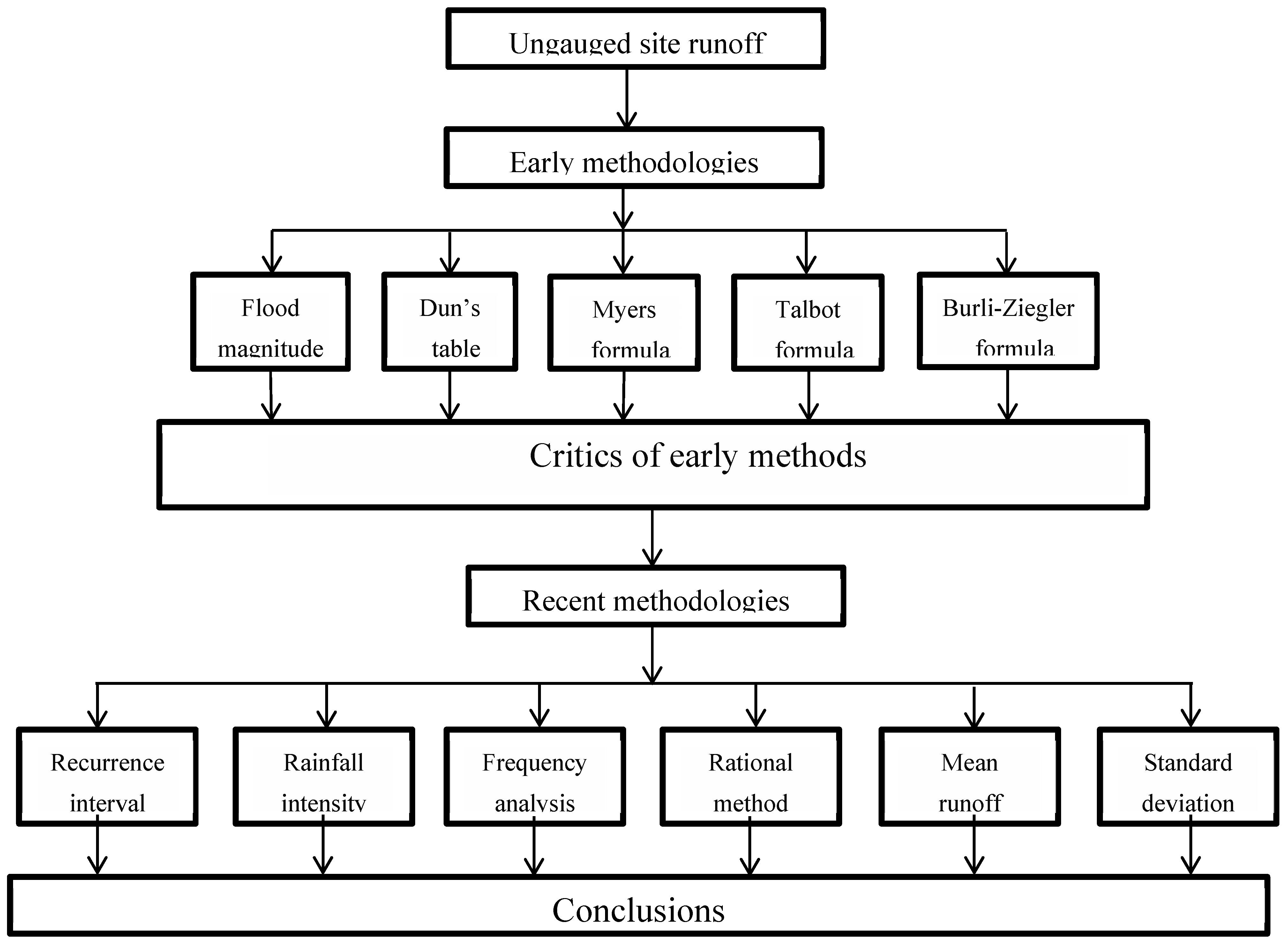
The brief content of this paper is presented in Figure 1 for a clear visualization and appreciation of the logical connections between different sections and sub-sections.
2. Early Methodologies
Blanchard and Drowne [9] advocated the use of empirical methods or formulas developed over time from local observations. They correctly observed that methods that consider drainage area alone cannot provide universally satisfactory results. Valuable data on the proper size of any particular culvert may be obtained through consideration of the following points [8].
- (1)
- Observing the existing openings on the same stream;
- (2)
- Measuring, preferably at time of high water, a cross-section of the stream at some narrow place; and
- (3)
- Determining the height of high water as indicated by drift and the evidence of the inhabitants of the neighborhood. With these data and a careful consideration of the various matters, it is possible to determine the proper area of the waterway with a reasonable degree of accuracy.
There are a number of empirical formulae which provide extremely different results from each other because each one was developed for a specific location. Some of these formulae have only one variable, namely= the drainage area, and we cannot expect that the results of such formulae will agree with those obtained by formulae that have coefficients to be applied for different soil conditions, steepness of slope, etc. [9].
2.1. Flood Magnitude and Economics
Early hydrologists differed in their opinions on the acceptable frequency of roadway flooding. One of the earliest American textbooks on road building stated that hydrologically, culverts should be sized for the worst-case scenario [10]. Their size must be proportioned to the greatest quantity of water, which can ever be required to pass, and should be at least 18 inches square, or large enough to admit a boy to enter to clean them out. However, most early textbooks on highway engineering hydrology advocated consideration of the economic trade-offs in the sizing of hydraulic structures (culverts and bridges).
Special care is required to provide an sufficient way for the water to pass. If the sizing is too small, it is liable to cause a washout, entailing environmental losses, repair costs, and possible accidents that will require payment of large sums for damages. On the other hand, if the design is made unnecessarily large, the cost of construction is needlessly increased. Anyone can make a design large enough, but it is the province of the hydrologist to design one of sufficient but not extravagant size [8].
The economy of designing a water structure to take the maximum discharge from an area should be determined by considerations of the upstream basin features. It would be uneconomical to build the structure to meet maximum conditions if the interest on the first cost was less than the cost to repair the damage incurred by the use of a structure furnishing a smaller waterway. Where a loss of life would be involved, however, the structure should be designed to meet maximum conditions [9].
The first step to take is to decide on what magnitude of flood may occur. Extreme floods may occur, but once or twice in a century, and the cost of caring adequately for such a contingency is excessive and unwarranted in many instances. Here, the best judgment of the engineer will be needed, because the temptation will be to use too rigidly the principle that the loss due to an extreme flood is justified if it does not exceed the capitalized cost of the additional waterway necessary to prevent it. The difficulty in applying this principle is to foresee all the items that will enter into some future loss, and thus arrive at a true aggregate. The engineer should be liberal in assuming the magnitude of the discharge to be provided for, as well as in forecasting the probable amount of damage that in the future might be caused by an abnormally great flood [11].
As stated by Chatburn [12], it may not always be wise to provide for extreme cases of high water that have occurred only once in a generation; it may be cheaper to risk the washing out of a road or culvert.
2.2. Dun’s Table
The most popular early methods for hydrologic design of drainage structures included Dun’s table, the Myers and Talbot formulas for waterway area, and the Burkli-Ziegler formula for discharge. The first significant generation of hydrological procedures were due to railroad engineers; in particular, they developed and published numerous tables and formulas for waterway sizing, for which the early table was presented by the chief engineer of the Atchison, Topeka and Santa Fe Railway [13]. Later, a comprehensive report on waterway sizing was published by the American Railroad Engineering and Maintenance of Way Association (AREMWA) [14] in 1911, and it presented six formulas for waterway areas and 21 formulas for design discharge. A historical review of waterway sizing methods by Chow [15,16] lists 12 formulas for waterway areas and 62 formulas for design discharge.
The engineer’s judgment with respect to choice of formulae for sectional areas of stream would be to discard them all and use Dun’s table, which gives data based on actual records up to areas of 6500 square miles [11].
2.3. Myers Formula
Cleeman [17] wrote about the Myers formula for waterway areas which was first published in the Proceedings of the Engineers Club of Philadelphia in 1879. The Myers formula is given as follows:
where A is the area of waterway (ft2), D is the drainage area (acres), and C is a coefficient recommended to be 1.0 as a minimum for flat lands, 1.6 for hilly compact ground, 4.0 as a minimum for mountainous and rocky lands, and higher values in exceptional cases.
Equation (1) can be converted to surface runoff discharge, Q, estimated for ungauged sites by multiplying it with the flow velocity, V, which leads to the following expression:
If the flow velocity is adapted in units of ft/s, then the discharge will result in ft3/s. The application of this expression requires an expert view of the water structure location.
Meyers developed his formula from observations of structures in the general vicinity of the railroad line. Following its publication, the Myers formula was used to a great extent by railroad engineers in the eastern part of the United States [9], and was included in several early texts on highway engineering. However, the Myers formula does not appear to have been widely adopted by highway engineers.
2.4. Talbot Formula
The Talbot [18] formula was first proposed before the turn of the 20th century, when practically nothing was known regarding hydrology or hydraulic design. Its widespread adoption can be attributed probably to its simplicity and the lack of something better. The 1911 AREMWA report on waterway sizing stated that “the Talbot formula had been very generally adopted, particularly in the West and in the southwestern portion of the country”. The highway departments of 25 states including Kansas listed the Talbot formula as an acceptable design method in the University of Illinois’s 1953 survey of design practices [19]. The Talbot formula gained widespread popularity among railroad and highway engineers. Talbot’s formulation has the following mathematical form.
where A is the area of waterway (ft2), D is the drainage area (acres), and C is a coefficient. Talbot offered the following guidance for selection of the coefficient, C.
- (i)
- For rolling agricultural country, subject to floods at the time of melting snow, and with the length of valley three or four times the width, one third is the proper value for C;
- (ii)
- In districts not affected by snow, and where the length of the valley is several times the width, one-fifth or one-sixth or even less may be used; and
- (iii)
- C should be increased for steep side slopes, especially if the upper part of the valley has a much greater fall than the channel at the culvert.
In any case, judgment must be the main dependence, the formula being a guide to it. On a road already constructed, the C may be determined for the character of surface along that line by comparing the formula with the high water mark of a known drainage area. Experience and observation on similar water courses are the most valuable guides. Knowledge of the action of streams of similar situations in floods and of the effects of peculiar formations is of far more value than any extended formula [18]. In a subsequent discussion, Talbot added the statement that “For steep and rocky ground, C varies from two-thirds to unity”.
The Modified Talbot empirical formulae, after Quraisi and Al-Hasoun [20], give the peak discharge for different sizes of large watershed as follows:
Q25 = 4.985 C(A)0.5
Q50 = 1.2Q25
Q100 = 1.17 Q50
Parameters Q25, Q50, and Q100 are runoff discharges (m3/s) for return periods of 25 years, 50 years and 100 years, respectively. Parameter C is for summation of C1, C2 and C3 which depends on terrain condition, slope, width, and length of drainage area (see Table 1) and A is drainage area in hectares.
The Modified Talbot method is popular for design of hydraulics structures even recently in the Kingdom of Saudi Arabia. However, many hydrologists disagree with it, because (i) the modification factors used are excessive (0.1 to 2.0) without clearly defined criteria, and (ii) the rainfall intensity is ignored for the estimation of flash floods in urban/developed areas.
Other points worth discussing on Modified Talbot method are as follows:
- (a)
- The same straight line is used to derive the 25 year return period discharge as Q25 = Qbasis S, where S is the slope of wadi main channel. This implies that as long as the slopes and the wadi drainage areas are the same, the discharge value can be obtained, irrespective of location anywhere in the world. However, this cannot hold true for any location. It has already been stated that there should be some difference in the discharge between arid regions and humid regions [22];
- (b)
- The 25 year return period discharge is converted to discharges for other periods (50 year, 100 year, etc.) using the same constant multiplications. These constants can be derived at least from rainfall records in a particular area according to some suitable theoretical probability distribution functions (PDF), such as extreme value distribution functions. These constants cannot be adopted by taking the same value for use in different areas of the regions;
- (c)
- The Modified Talbot formulation does not take into consideration the rainfall intensity/design of the storm based on return period;
- (d)
- Runoff coefficient (C) has maximum value of 0.9 when taking into consideration bedrock nature, channel slope, and some topographic factors. Coefficient factors, C1, C2 and C3 are not mathematical expressions and thus cannot be adapted as constants for the whole catchment. The reason for this is that any catchment may have mixed land use which varies according to topography and mountainous areas, vegetation cover, low lands, urban areas, rural areas, and residential areas. The Talbot approach has a limited choice of land-use types and this makes its application questionable, particularly in arid regions with mountainous settings; and
- (e)
- The Modified Talbot formulation does not take into consideration the percentage of imperviousness, soil infiltration parameters (i.e., initial and constant losses) and transformation parameters (i.e., time of concentration and storage coefficient) within the catchment. On the other hand, the time of concentration is a very important parameter in hydrograph analysis and is estimated generally by empirical formulations based on watershed major channel length and slope values [23].
The method is not very well known in the hydrology and flood discharge calculation literature, and it is a more than 100 year old approach. At times in the past, there were not rainfall records, and hence many researchers sought simple empirical formulae; however, with meteorology instrumentations, rainfall records are frequently available in many areas of the world. The following points can be raised against this methodology.
- (i)
- It takes into consideration the area of drainage basin and then, according to this size, slope and shape empirical formulations are given with subjective specification. Basically, it yields a 25 year return period discharge, and then subsequent proposed factors are used for its increment to other return periods of 50 years, 100 years, etc. (see Equations (4)–(6)).
- (ii)
- Shape factor is another basic variable, but it is dependent on the areal width and area of the basin, hence it does not take into consideration the length of the major stream, which contributes to flood discharge more than any other drainage parameter.
- (iii)
- It does not take into consideration rainfall intensity. However, there are other methodologies that do not take into account rainfall intensity, but they are more recent (e.g., the Snyder [23] method, which has logical foundations). However, it is recommended in modern times that rainfall intensity is taken into consideration as the major factor in flood calculations.
- (iv)
- C, as the runoff coefficient, has been considered compositely as maximum values equal to 0.9. It is decided in a subjective manner by taking into consideration the bedrock nature, channel slope, and some topographic factors. In fact, nowadays, there are detailed tables for the determination of C depending on surface soil types, and for hydrological soil classification taking into consideration vegetation cover, land use, geology, topography, etc., in Chow [15], both of which are not considered in the Talbot approach,
- (v)
- It is not clear how the Discharge (Q)-Area (A) straight line is obtained on double logarithmic paper. Accordingly, the basic equation Q25 = QbasicS.F takes only into consideration the area. Inclusion of S.F. is not clear, although it is mentioned that it is dependent on the slope factor for the drainage area.
- (vi)
- W is a factor that reflects the elongation ratio of the catchment, but not the drainage density and main channel slope, which are important in discharge calculations.
- (vii)
- There is no reason why n is taken as 3/4 (see Equation (3)); in fact, there should be some empirical basis for such an exponent. In the Saudi Geological Survey (SGS) reports, this figure is based on factual data, and the exponent appears as 0.522.
- (viii)
- C1, C2 and C3 are based on expert views and not mathematical expressions. They cannot be taken as constants for the whole catchment, because in any catchment there may be a mixture of mountainous areas, vegetation cover and low lands. Perhaps the best figure that can be used is the weighted average, but such an approach is not available in the Talbot method.
- (ix)
- The factors for Q50 = 1.2Q25 and Q100 = 1.4Q25 can be considered frequency factors, but they should be based on a certain probability distribution function (PDF) such as Gumbel, Pearson Type-II, log-Pearson, or extreme value distributions with validation. These factors cannot be adopted as constant in the different areas of a region. Additionally, they should also be dependent on the rainfall PDF.
- (x)
- The width, W, of the wadi is taken as constant, for a given discharge, as W = 4.84√Q; this should vary along the main channel of the wadi [22].
2.5. Burkli-Ziegler Formula
Burkli-Ziegler was a Swiss engineer, and published his formula for design discharge in 1880. Hering [24] introduced it to U. S. practice. The Burkli-Ziegler formula is given as follows.
in which Q is the discharge (cfs), C is a coefficient ranging from 0.31 to 0.75, depending on the nature of the surface; 0.62 is recommended for general use, r is the rainfall intensity (in/hr), S is the general grade of the area (ft/1000 ft), and A is the drainage area (acres). Equation (7) was the most popular of the early formulae for design discharge. It was originally developed for urban drainage applications, but it is not suitable for rural drainage basins.
2.6. Flood Frequency
The first major report on flood frequency for Kansas streams was prepared by the USGS and published by the Kansas Water Resources Board in 1960 [25]. This report presented the first regional flood–frequency relationships for Kansas. These relationships provided estimates of flood discharges with recurrence intervals up to 50 years, based on drainage area and geographic location, for unregulated streams with drainage areas over 150 mi2.
No regional relationships were provided for drainage areas under 150 mi2. The first regional flood–frequency relationships for small streams in Kansas were published by the USGS in 1966 [26]. These relationships for drainage areas under 70 mi2 were labeled “preliminary” because they were based on only 8 years of peak flow data (1957–1964) for 95 stations. The report presented statewide regression equations for discharges with recurrence intervals of 1.2 years, 2.33 years (the mean annual flood for a Gumbel [27] probability distribution), 5-years and 10-years. The three inputs to these equations are drainage area, average channel slope, and the average number of wet days per year. The standard error of estimation for the 10 year equation, expressed in percent, is from +100% to −49%. A more comprehensive USGS study of Kansas flood frequency, published by the Kansas Water Resources Board in 1975 [28] provided statewide equations for flood discharges with recurrence intervals from 2 years to 100 years for unregulated rural streams with drainage areas from 0.4 to 10,000 mi2. The two inputs to these equations are the drainage area and the 2 year, 24 h rainfall, which are obtained from a map. The standard errors range from +50% to −31% for the 5-year equations, and from +74% to −42% for the 100 year equations. The 1975 USGS equations were the first regional flood frequency equations to be widely used to compute design flows for highway culverts and bridges in Kansas. The USGS published updated flood-frequency equations for Kansas in 1987 Clement [29] and 2000 Rasmussen and Perry [30]. The 1987 equations have four inputs: drainage area, 2 year 24 h rainfall, average channel slope and generalized soil permeability. The 2 year 24 h rainfall and the generalized soil permeability are obtained from maps. Standard errors range from +35% to −26% for the 10 year equations, and from +46% to −31% for the 100 year equations.
The latest update, published in 2000, provides two sets of statewide flood frequency equations: one for drainage areas over 30 mi2 and another set for drainage areas under 30 mi2. The equations for drainage areas over 30 mi2 have four inputs: drainage area, mean annual precipitation, channel slope and generalized soil permeability. Standard errors range from +35% to −26% for the 10-year equations, and from +42% to −30% for the 100 year equations. The equations for drainage areas under 30 square miles have only two inputs: drainage area and mean annual precipitation. These equations for small watersheds have large standard errors that vary from +52% to −34% for the 10-year and from +71% to −41% for the 100-year equations.
2.7. Critics of Early Methods
Even early hydrologists and engineers were well aware of the shortcomings and uncertainties of their hydrologic design methods. Most of the early methods were based on a rule of thumb. However, it is preferable to suggest simple and logical rules, where there is no rule rather than potentially causing problems, and one must confess doubts as to whether this is not the case with the various formulae. Early hydrologists and engineers were also aware that there are uncertainties in their formulations, because of the probable variations in maximum rainfall and possible future changes in the conditions of the drainage basin surfaces. This is the main reason why numerous approximate empirical formulae have been proposed, as no formula can give accurate results with inaccurate data [8]. He offered the following observation on the precision required in the sizing of drainage structures.
The determination of the values of the different factors entering into the problem is almost wholly a matter of judgment. An estimate for any one of the above factors is liable to be in error from 100% to 200% percent, or even more, and of course any result deduced from such data must be very uncertain. Fortunately, mathematical exactness is not required by the problem nor warranted by the data. The question is not one of 10% or 20% of increase; for if a 2 m3/s is insufficient, a 3 m3/s design discharge may be considered and this will mean an increase of 225%. The real question is which one to adapt in practical applications.
There are various ways, however, in which the amount of water and the size of opening can be determined. The variables which enter into the problem make the results more or less approximate, and different formulas may give widely varying results for the same conditions. In any event, the use of such results is better than a mere guess, and if some method or formula can be applied to conditions in any one locality for a sufficient length of time, then proper study can be given to the factors, which tend to make the results approximate. In time, the method or formula can be depended upon to give results, which for that particular locality at least are reasonably accurate.
Unfortunately, many of the early formulations are widely divergent, mainly because of variations in the governing conditions, such as the area of drainage basin, amount of annual rainfall and its intensity, the extent and duration of rain storms, the slope of stream and its tributaries, the character of soil and the quality and extent of vegetation. These factors certainly constitute a valid excuse for considerable divergence in the resulting values of stream areas and discharges as calculated by the various formulae that have received more or less endorsement from the engineering profession; however, they are by no means a legitimate reason for the ridiculously large variations that one notes when applying such formulae for a particular case.
3. Recent Methodologies
Modern methods for the sizing of water structures are based on frequency analysis of streamflow and/or rainfall data; i.e., structures are sized for a flood with a specific recurrence interval. Research by the Bureau of Public Roads and others in the 1940s laid the groundwork for frequency-based sizing of culverts and bridges. Gumbel [27] published the first book on how to estimate extreme floods based on the PDF. The transition to frequency-based design in highway engineering practices occurred mainly in the 1950s.
The first highway engineering textbook to advocate the modern approach to waterway sizing was due to Hewes and Oglesby [31]. The following paragraph from the Foreword signaled the new approach.
“In the past, hydrologic data of value to highway engineers have been fragmentary, and hydraulic designs based on them often seemed pointless. For this and other reasons, drainage design before about 1940 was largely by rule-of-thumb methods, many of them with doubtful validity. Since that time, and particularly since World War II, highway engineers have devoted increasing attention to drainage problems. Research already completed or underway will greatly extend present knowledge. The results of these efforts are already and will be increasingly apparent in better and more economical highway drainage. This textbook offered the following lucid explanation of the role of probability in hydrologic design”.
It should be understood at the outset that predictions regarding future rainfall or runoff from accumulated records rest on the laws of probability methodology. To illustrate, consider the statement that a culvert is designed to carry a “50 year” flood. This means that, if past experience is repeated, the chances are 1 in 50 that the structure will flow full or be overtaxed once in a particular year. It does not mean that the design flood or a larger one will occur exactly one time in 50 years; in fact, the chances are only 64 in 100 that a flood of this magnitude will occur in a given 50-year period. On the other hand, several floods of this or greater magnitude could occur in successive years or in a single year, but the chance of either combination is extremely small.
The Hewes and Oglesby [31] textbook presented two methods for estimation of design flows with specified recurrence intervals: the Bureau of Public Roads method (Izzard [32] and the rational method (RM). It also included a brief discussion of unit hydrographs and their uses in highway engineering.
In the 1960s, the USGS and other agencies began to develop regional flood-frequency relations using regression analysis rather than graphical methods. These regional regression equations were widely adopted for estimation of design flows on unregulated rural streams. New regression equations are developed periodically to incorporate new data.
In the late 1960s, a National Cooperative Highway Research Program project attempted to develop nationwide regression equations for flood discharges on small rural streams [33].
3.1. Recurrence Intervals for Design
The University of Illinois’s 1953 survey of the design practices of state highway departments showed little agreement on recurrence intervals for bridges and culverts at the start of the modern era [19]. The recurrence intervals reported for “bridges, large culverts, and the drainage structures in the primary highway system” ranged from 5 to 100 years. The most common recurrence interval for these larger or more important structures was 50 years.
The Bureau of Public Roads first implemented frequency-based design criteria for drainage structures on interstate highways in 1956. These design criteria specified a minimum recurrence interval of 50 years for drainage structures on interstate highways. The federal government has never specified minimum recurrence intervals for drainage structures on interstate highways.
3.2. Rainfall Frequency
The first reliable rainfall-frequency maps for daily and longer-duration rainfalls were published in 1917 by the Miami (Ohio) Conservancy District in a report titled Storm Rainfall of Eastern United States [34]. These maps provide rainfall estimates for durations of one to six days and recurrence intervals of 15 to 100 years for the United States east of the 103rd meridian, which includes all of Kansas.
The first reliable rainfall-frequency estimates for shorter durations were published in 1935 by the U.S. Department of Agriculture in a report titled Rainfall Intensity-Frequency Data [35,36]. This report provides nationwide rainfall maps for durations from 5 min to 24 h and recurrence intervals from 2 to 100 years. This system is used even in today’s hydrological design applications. The next significant report on rainfall frequencies for the eastern and central United States was the U. S. Weather Bureau’s Technical Paper No. 40, “Rainfall Frequency Atlas of the United States”, published in 1961 [37]. This work remains the most widely accepted source of rainfall estimates for durations over one hour.
The Rational Method (RM), the Soil Conservation Service [38,39] methods and others require rainfall frequency information. The SCS Runoff Curve Number Method, developed by the USDA Soil Conservation Service, is one of the most important hydrologic runoff estimation methods, and has support and criticism. Reasonably accurate rainfall frequency information for Kansas, covering the durations and recurrence intervals needed for highway applications, has been available since the U. S. Department of Agriculture published its nationwide report on rainfall frequency in 1935 [36].
KDOT’s Rainfall Tables for Counties in Kansas was originally developed from the rainfall frequency maps in Technical Paper 40 [37]. These rainfall tables were revised in 1992 to incorporate the improved estimates for short duration rainfalls from HYDRO-, and re-issued with minor corrections in 1997.
The most up-to-date rainfall frequency estimates for the Kansas City metropolitan area are those published by the Kansas City Metro Chapter of the American Public Works Association in 2002 [40]. The rainfalls depths in this report are larger than the values in the NWS atlases for short durations and long recurrence intervals (up to 14% higher for the 10 min, 100 year event) and lower for short durations and short return periods (13% lower for the 5 min, 2 year event). These differences are due primarily to differences in statistical methods.
3.3. Flood Frequency Analysis
The modern era of flood frequency analysis began in the early 1940s with a series of groundbreaking papers by [27,41]. Before Gumbel, flood data were analyzed by ad hoc graphical methods. Gumbel developed a theoretically sound method based on fitting an extreme value Type I PDF to the record of annual peak flows.
In the 1970s, the U. S. Water Resources Council (USWRC) developed recommended procedures for flood frequency analysis to be applied by all federal agencies. In the USWRC method of flood frequency analysis, the record of annual flood peaks are fitted with a log-Pearson Type III PDF rather than Gumbel’s extreme value probability distribution.
4. Practical Estimation Methodologies
4.1. Rational (RM) Method Versions
Although this has been defined as the drainage area ratio (DAR) technique that assumes the equality of the flow per unit area, or unit discharge between hydrologically similar catchments, its physical reasoning can be derived from the rational method (RM) for estimation of discharge, Q, which states that
where C is the runoff coefficient, I is the rainfall intensity and A is the drainage area.
According to Dooge [42], the RM for calculation of design discharges was first described by Irish engineer [43]. The method was introduced to the United States by Kuichling [44], but it did not become popular with highway engineers until much later. The lack of reliable guidance for the estimation of the runoff coefficient, time of concentration and rainfall intensity probably explains why the RM was not embraced by early highway engineers.
If the two similar basins are X and Y, then by using these subscripts, Equation (8) can be re-written for each basin as follows.
and
The ratio of these formulations yields
The runoff coefficient selection for lawns is presented in Table 2, depending on the land use.
It is possible to prepare a table for the runoff coefficients ratios, CX/CY, from Table 2, leading to Table 3.
If one assumes that in both basins the runoff coefficients and the rainfall intensities are equal to each other, it is possible to derive from Equation (11) that
which is equivalent with the DAR suggestion in Equation (8) of Farmer and Vogel [45]. Hence, their Equation (8) has a set of assumptions:
- (i)
- The runoff coefficients are equal, which is hardly the case in practical applications due to the differences in geomorphology, land use, geologic lithology and vegetation cover, etc.;
- (ii)
- Equal rainfall intensities generate equal discharges per area in both basins; and
- (iii)
- Since the RM is valid only for small drainage basins [16], the validity of Equation (11) has areal limitation.
It is possible to improve Equation (12) so as to take into consideration the difference at least in the runoff coefficients, and a ratio coefficient, α, can be imported. Therefore, one can obtain
However, as the authors rightly state in some practical applications, a power constant, n, is considered, and the same expression can be rewritten as follows.
Logically, 0 < n <1, and as the similarity between the two basins increases, n approaches 1. If they are identically the same, then n = 1 and the DAR formulation becomes valid with the above restrictions as assumptions.
Apart from all the aforementioned physical and logical explanations, the DAR equation can also be written by including an error term, ε, which also distinguishes the two basins to a certain extent.
where ε, has zero mean and unit standard deviation, and abides by the normal PDF.
4.2. Mean Runoff Versions
This is referred to as the standardized mean (SM) technique by Farmer and Vogel (2013), again without logical explanation. If one considers the simplest form of stochastic process as the first order Markov model for streamflow generation, then one can write the following for a given discharge time series (Qi; Q1, Q2, ⋯, Qn) at a site:
where μi is the arithmetic average, σi is the standard deviation, ρi is the first order serial correlation coefficient, and finally εi is the standard normal PDF with zero mean and unit standard deviation. It is mentioned by Farmer and Vogel [45] that such an approach is used in flood frequency analysis. This statement implies that the serial correlation coefficient is equal to zero, which reduces Equation (16) into the following form.
If one assumes that there is only the effect of arithmetic mean and ignores the contribution by the standard deviation, the last expression can be written as follows.
Finally, this expression can be considered for the gauged, X, and ungauged, Y, sites; their ratio leads to
This is the expression for the SM method, and one can appreciate the assumptions behind its derivation. Logically, compared with the DAR approach, SM has wider validity, because it does not have any restrictive areal extend.
4.3. Mean Runoff and Standard Deviation Versions
The standardization of flows by mean and standard deviation (SMS) works on a dimensionless discharge variable for which the expectation value is zero and the variance is equal to the unit. The basis of its derivation is again the first order Markov model, and the assumption of serial independence, which led to Equation (18). Rearrangement of this expression leads to
which implies that at each time instant, the mean and standard deviation are taken into consideration, hence only residuals remain. This expression also confirms the statement by Farmer and Vogel [45] that a new standardized variable is obtained with zero mean and unit variance, regardless of the PDF of the original flows. The ratio of this last expression between the gauged, X, and ungauged, Y, sites gives
If one assumes that at the two sites, the error terms are also the same, this last expression reduces to
Since this approach, SMS, takes into account standard deviation in addition to arithmetic average, as Farmer and Vogel [45] state, it is directly superior to the drainage area ratio method (DAR) because its amount information content is greater than even the SM method. The consequent logical deduction is that SMS is expected to yield better results than even SM. After all, for the information content concerning streamflow sequence, it is possible to rank these approaches into a sequence of preference: DAR < SM < SMS. Such a sequence has already been observed in the numerical calculations [45]. Comparisons between early and recent runoff methodological estimation approaches are presented already throughout the text.
5. Conclusions
In the early days of highway construction, culverts and bridges were sized by empirical methods developed from experiences with existing structures during floods. Most of these methods were developed for the railroads. No particular recurrence intervals were associated with the resulting designs. Early highway engineers were aware of the shortcomings of these design methods, but they were hampered by a shortage of reliable streamflow and rainfall data. The transition to modern frequency-based design methods generally occurred during the 1950s.
The highway building era in Kansas began in 1917 with the establishment of the Kansas State Highway Commission (KSHC). Prior to the mid-1950s, most culverts and bridges on Kansas highways were sized with the Talbot formula, Dun’s table and other empirical methods. The KSHC and Kansas Department of Transportation (KDOT) have employed frequency-based design methods such as the Rational Method (RM) and USGS regression equations since the 1960s. Highway culverts and bridges have been designed for recurrence intervals of 25 years or greater. The hydrologic methods and design guidelines employed by KSHC and KDOT have been within the mainstream of highway engineering practice. Hydrologic methods have been improved as more streamflow data become available. However, flood frequency estimates for small watersheds still have large standard errors.
The engineering profession’s understanding of culvert and bridge hydraulics has advanced greatly over the last century. The Talbot formula, Dun’s table and similar empirical design methods did not explicitly consider the hydraulic characteristics of the structure. Modern design methods require hydraulic analyses that started to appear in the literature around 1945. This paper first presents the evolution of the ungagged drainage basin discharge formulations starting from the second half of the 19th century. In the second part, some practically applicable recent ungauged drainage methodologies are presented.
In future, flood early warning procedures must be constructed in such a way as to increase public awareness and enhance and improveintegrated flood management (IFM) systems and flood resilience, defined as the ability of a system and its components to anticipate, absorb, accomodate and recover from the effects of hazardous event in timely and efficient ways. The limitation of the ungauged site runoff estimation is confined to the absence of numerical data and verbal communication systems, which are necessary components for better modeling and local public and administrator planning studies.
Funding
This research received no external funding.
Data Availability Statement
Data is available at any request.
Conflicts of Interest
The authors declare no conflict of interest.
References
- Kansas Water Commission. Surface Waters of Kansas, 1895–1919; Kansas Water Commission: Topeka, KS, USA, 1920. [Google Scholar]
- Kansas Water Commission. Surface Waters of Kansas, 1919–1924; Kansas Water Commission: Topeka, KS, USA, 1928. [Google Scholar]
- Şen, Z. Flood Modeling, Prediction, and Mitigation; Springer: Berlin/Heidelberg, Germany, 2018; 422p. [Google Scholar]
- McEnroe, B.M. Sizing of Highway Culverts and Bridges: A Historical Review of Methods and Criteria; Final Report No. K-TRAN: KU-05-4; Kansas Department of Transportation: Topeka, KS, USA, 2007; pp. 1–45. [Google Scholar]
- Ibrahim, B.; Wisser, D.; Barry, B.; Fowe, T.; Aduna, A. Hydrological predictions for small ungauged watersheds in the Sudanian zone of the Volta basin in West Africa. J. Hydrol. Reg. Stud. 2015, 4, 386–397. [Google Scholar] [CrossRef]
- Kim, D.Y.; Song, C.M. Developing a discharge estimation model for ungauged watershed using CNN and hydrological image. Water 2020, 12, 3534. [Google Scholar] [CrossRef]
- Park, G.T. A Study on Estimation of Runoff in Ungauged Sub-Watershed based on Soil Characteristics Sensitivity. Master’s Thesis, Incheon National University, Incheon, Korea, 2022. [Google Scholar]
- Byrne, A.T. A Treatise on Highway Construction, 4th ed.; John Wiley & Sons: New York, NY, USA, 1902. [Google Scholar]
- Blanchard, A.H.; Drowne, H.B. Text-Book on Highway Engineering; John Wiley & Sons: New York, NY, USA, 1913. [Google Scholar]
- Gillespie, W.M. A Manual of the Principles and Practices of Road Making: Comprising the Location, Construction, and Improvement of Roads and Railroads, 6th ed.; A.S. Barnes & Co.: New York, NY, USA, 1853. [Google Scholar]
- Waddell, J.A.L. Determination of Waterways. In Bridge Engineering 2; John Wiley & Sons: New York, NY, USA, 1916; pp. 1109–1136. [Google Scholar]
- Chatburn, G.R. Highway Engineering: Rural Roads and Pavements; John Wiley and Sons: New York, NY, USA, 1921. [Google Scholar]
- Bremner, G.H.; Dun, J.; Alvord, J.W.; Talbot, A.N. Symposium on Methods of Determining the Size of Waterways. J. West. Soc. Civ. Eng. 1906, 11, 137–190. [Google Scholar]
- AREMWA. Report of the Sub-Committee of Roadway Committee No. 1; Bulletin 131; Part 3; American Railway Engineering and Maintenance of Way Association: Lanham, MD, USA, 1911; Volume 12, pp. 481–528. [Google Scholar]
- Chow, V.T. (Ed.) . Handbook of Applied Hydrology; McGraw-Hill Book Publishing Company: New York, NY, USA, 1964. [Google Scholar]
- Chow, V.; Maidment, D.; Mays, L. Applied Hydrology; McGraw-Hill: New York, NY, USA, 1998; 572p. [Google Scholar]
- Clement, R.W. Floods in Kansas and Techniques for Estimating Their Magnitude and Frequency on Unregulated Streams; Water-Resources Investigations Report 87-4008; U.S. Geological Survey: Reston, VA, USA, 1987. [Google Scholar]
- Talbot, A.N. The Determination of Water-Way for Bridges and Culverts; Engineers’ Club, Technograph No. 2; University of Illinois: Champaign, IL, USA, 1888; pp. 14–22. [Google Scholar]
- Chow, V.T. Hydrologic Determination of Waterway Areas for Design of Drainage Structures in Small Drainage Basins; Engineering Experiment Station Bulletin No. 462; University of Illinois: Champaign, IL, USA, 1962. [Google Scholar]
- Quraishi, A.A.; Al-Hassoun, S.A. Use of Talbot formula for estimating peak discharge in Saudi Arabia. J. King Abdulaziz Univ. 1996, 8, 73–75. [Google Scholar] [CrossRef]
- Wilson Murrow Consultant. Drainage Report. A Report Submitted to the Ministry of Communications; Wilson Murrow Consultant: Riyadh, Saudi Arabia, 1971; 217p. [Google Scholar]
- Şen, Z. Wadi Hydrology; Taylor and Francis Publishers: Boca Raton, FL, USA; CRS Press: Boca Raton, FL, USA, 2008; 347p. [Google Scholar]
- Kirpich, Z.P. Time of concentration of small agricultural watersheds. Civ. Eng. 1940, 10, 362. [Google Scholar]
- Hering, R. Sewerage Systems. Trans. Am. Soc. Civ. Eng. 1881, 10, 361–384. [Google Scholar] [CrossRef]
- Snyder, F. Synthetic Unit-Graphs. Eos Trans. Am. Geophys. Union 1938, 19, 447–454. [Google Scholar] [CrossRef]
- Ellis, D.W.; Edelen, G.W., Jr. Kansas Stream Flow Characteristics. Part 3: Flood Frequency; Technical Report No. 3; Kansas Water Resources Board: Manhattan, KS, USA, 1960. [Google Scholar]
- Gumbel, E.J. Floods Estimated by Probability Method. Eng. News-Rec. 1945, 134, 97–101. [Google Scholar]
- Jordan, P.R.; Irza, T.J. Kansas Streamflow Characteristics: Magnitude and Frequency of Floods in Kansas, Unregulated Streams; Technical Report No. 11; Kansas Water Resources Board: Manhattan, KS, USA, 1975. [Google Scholar]
- Cleeman, T.M. Proper Amount of Water-Way for Culverts; Engineers’ Club of Philadelphia: Philadelphia, PA, USA, 1879; Volume 1, pp. 146–149. [Google Scholar]
- Rasmussen, P.P.; Perry, C.A. Estimation of Peak Streamflow for Unregulated Rural Streams in Kansas, Water-Resources Investigations; Report 00-4079; U.S. Geological Survey: Reston, VA, USA, 2000. [Google Scholar]
- Hewes, L.I.; Oglesby, C.H. Highway Engineering; John Wiley and Sons: Hoboken, NJ, USA, 1954. [Google Scholar]
- Izzard, C.F. Peak Discharge for Highway Drainage Design. Trans. Am. Soc. Civ. Eng. 1953, 119, 1005–1015. [Google Scholar] [CrossRef]
- Bock, P.; Enger, I.; Malhotra, G.P.; Chisholm, D.A. Estimating Peak Runoff Rates from Ungauged Small Rural Watersheds; National Cooperative Highway Research Program Report No. 136; Highway Research Board, National Research Council: Washington, DC, USA, 1972. [Google Scholar]
- MCD, Miami Conservancy District. Storm Rainfall of the Eastern United States; Technical Reports; Part V; MCD: Dayton, OH, USA, 1917. [Google Scholar]
- Yarnell, D.L.; Woodward, S.H.; Nagler, F.A. The Flow of Water Through Pipe Culverts, Public Roads 5, No. 1; Bureau of Public Roads: Washington, DC, USA, 1924; pp. 19–33. [Google Scholar]
- Yarnell, D.L. Rainfall Intensity-Frequency Data, Miscellaneous Publication No. 204; U.S. Department of Agriculture: Washington, DC, USA, 1935. [Google Scholar]
- Hershfield, D.M. Rainfall Frequency Atlas of the United States for Durations from 30 Minutes to 24 Hours and Return Periods of 1 to 100 Years; Technical Paper No. 40; U.S. Weather Bureau: Silver Spring, MD, USA, 1961. [Google Scholar]
- Soil Conservation Service (SCS). Hydrology National Engineering Handbook; Section 4; Chapter 10; Soil Conservation Service, USDA: Washington, DC, USA, 1971. [Google Scholar]
- Soil Conservation Service (SCS). Hydrology National Engineering Handbook; Soil Conservation Service, USDA: Washington, DC, USA, 1982. [Google Scholar]
- Young, C.B.; McEnroe, B.M. Precipitation Frequency Estimates for the Kansas City Metropolitan Area; Kansas City Metropolitan Chapter; American Public Works Association: Kansas City, MO, USA, 2002. [Google Scholar]
- Smith, R.L. Hydrologic Design Utilizing Frequency-Equivalent Hydrographs; Report to Kansas Department of Transportation; Department of Civil Engineering, University of Kansas: Lawrence, KS, USA, 1982. [Google Scholar]
- Dooge, J.C.I. The Rational Method for Estimating Flood Peaks. Engineering 1957, 184, 311–313. [Google Scholar]
- Mulvany, T.J. On the Use of Self-Registering Rain and Flood Gauges in Making Observations of the Relations of Rainfall and Flood Discharges in a Given Catchment. Trans. Inst. Civ. Eng. Irel. 1851, 4, 18. [Google Scholar]
- Kuichling, E. The Relation Between Rainfall and the Discharge of Sewers in Populous Districts. Trans. Am. Soc. Civ. Eng. 1889, 20, 1–56. [Google Scholar] [CrossRef]
- Farmer, W.; Vogel, R.M. Performance-weighted methods for estimating monthly streamflow at ungauged sites. J. Hydrol. 2013, 477, 240–250. [Google Scholar] [CrossRef]
Figure 1.
Content flow chart.


Table 1.
Values of C1, C2 and C3 [21].
Table 1.
Values of C1, C2 and C3 [21].
| C1 | 0.30 | Mountainous area |
| 0.20 | Semi-mountainous | |
| 0.10 | Low land | |
| C2 | 0.50 | S > 15% |
| 0.40 | 10% < S < 15% | |
| 0.30 | 5% < S < 10% | |
| 0.25 | 2% < S < 5% | |
| 0.20 | 1% < S < 2% | |
| 0.15 | 0.5% < S < 1% | |
| 0.10 | S < 0.5% | |
| C3 | 0.30 | W = L |
| 0.20 | W = 0.4 L | |
| 0.10 | W = 0.2 L |
Note: W-width, L-length S-slope of drainage area.
Table 2.
Runoff coefficient for lawns [16].
Table 2.
Runoff coefficient for lawns [16].
| Land Use | C |
|---|---|
| Sandy soil flat, (2%) | 0.05–0.10 |
| Sandy soil avg., (2–7%) | 0.10–0.15 |
| Sandy soil steep, (7%) | 0.15–0.20 |
| Heavy soil flat, (2%) | 0.13–0.17 |
| Heavy soil avg., (2–7%) | 0.18–0.22 |
| Heavy soil steep, (7%) | 0.25–0.35 |
Table 3.
CX/CY ratios.
| Ungauged | X | ||||||
|---|---|---|---|---|---|---|---|
| Gauged | Sandy Soil Flat, (2%) | Sandy Soil avg. (2–7%) | Sandy Soil Steep, (7%) | Heavy Soil Flat, (2%) | Heavy Soil avg., (2–7%) | Heavy Soil Steep, (7%) | |
| Y | Sandy soil flat, (2%) | 1 | 0.5–0.67 (0.59) | 0.33–0.5 (0.43) | 0.77–0.59 (0.69) | 0.28–0.57 (0.43) | 0.20–0.29 (0.25) |
| Sandy soil avg., (2–7%) | 1 | 0.67–0.75 (0.71) | 0.77–0.88 (0.83) | 0.56–0.68 (0.62) | 0.40–0.43 (0.42) | ||
| Sandy soil steep, (7%) | 1 | 1.15–1.18 (1.17) | 083–0.91 (0.87) | 0.60–0.57 (0.59) | |||
| Heavy soil flat, (2%) | 1 | 0.72–0.77 (0.75) | 0.53–0.49 (0.51) | ||||
| Heavy soil avg., (2–7%) | 1 | 0.72–0.63 (0.68) | |||||
| Heavy soil steep, (7%) | 1 | ||||||
Disclaimer/Publisher’s Note: The statements, opinions and data contained in all publications are solely those of the individual author(s) and contributor(s) and not of MDPI and/or the editor(s). MDPI and/or the editor(s) disclaim responsibility for any injury to people or property resulting from any ideas, methods, instructions or products referred to in the content. |
© 2023 by the author. Licensee MDPI, Basel, Switzerland. This article is an open access article distributed under the terms and conditions of the Creative Commons Attribution (CC BY) license (https://creativecommons.org/licenses/by/4.0/).
Share and Cite
MDPI and ACS Style
Şen, Z. Hydrological Methodology Evolution for Runoff Estimations at Ungauged Sites. Water 2023, 15, 702. https://doi.org/10.3390/w15040702
AMA Style
Şen Z. Hydrological Methodology Evolution for Runoff Estimations at Ungauged Sites. Water. 2023; 15(4):702. https://doi.org/10.3390/w15040702
Chicago/Turabian StyleŞen, Zekâi. 2023. "Hydrological Methodology Evolution for Runoff Estimations at Ungauged Sites" Water 15, no. 4: 702. https://doi.org/10.3390/w15040702
Note that from the first issue of 2016, this journal uses article numbers instead of page numbers. See further details here.