
Comparison of Machine Learning and Traditional Statistical Methods in Debris Flow Susceptibility Assessment: A Case Study of Changping District, Beijing
Abstract
:1. Introduction
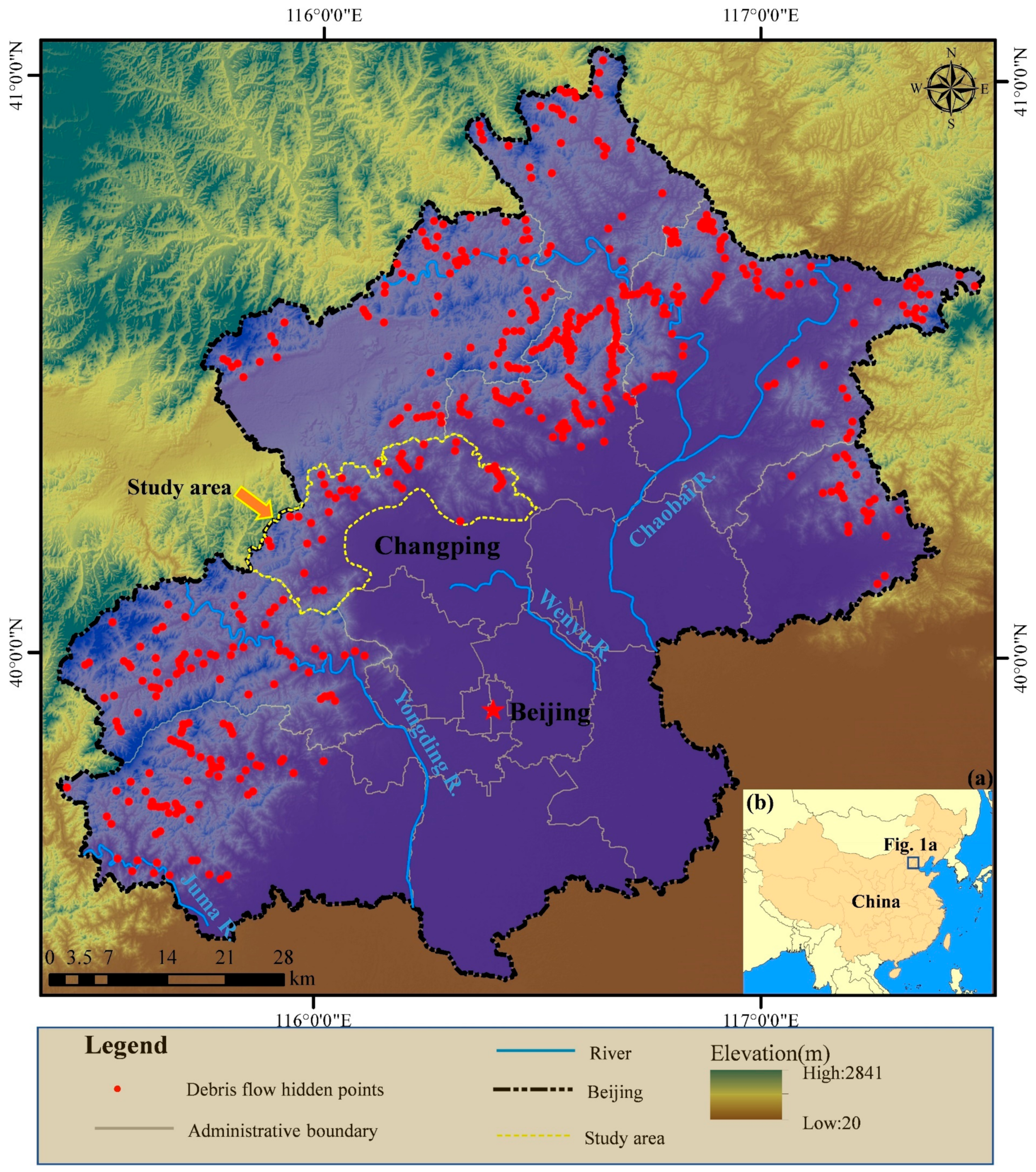
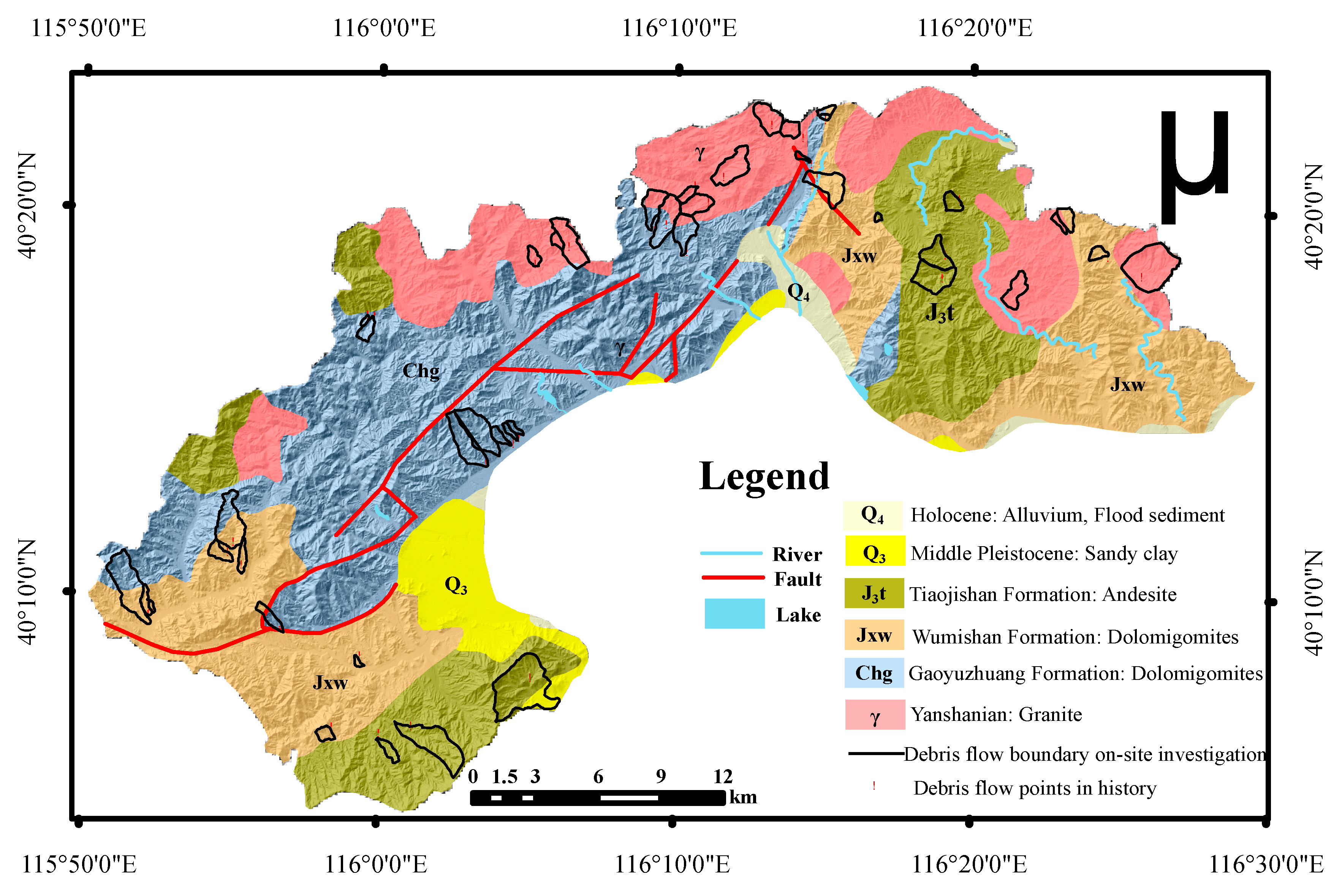
2. Study Area
3. Materials and Methods
3.1. Modeling Flow Chart
3.2. Mapping Unit
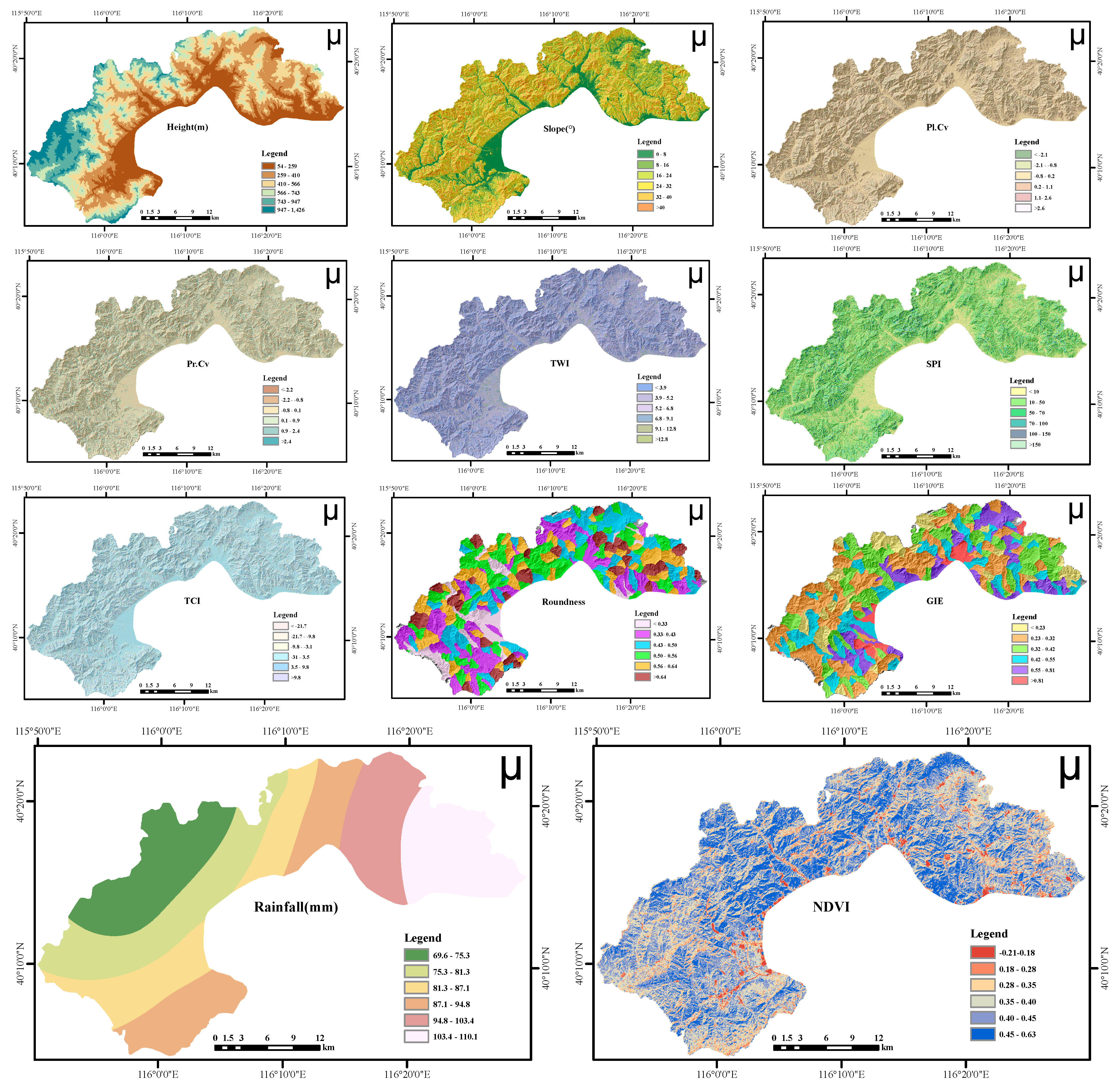
3.3. Determination of Causative Factors
3.4. Methods
3.4.1. Analytic Hierarchy Process (AHP)
3.4.2. Frequency Ratio (FR)
3.4.3. Principal Component Analysis (PCA)
3.4.4. Support Vector Machine (SVM)
3.4.5. Logistic Regression (LR)
4. Result Analysis
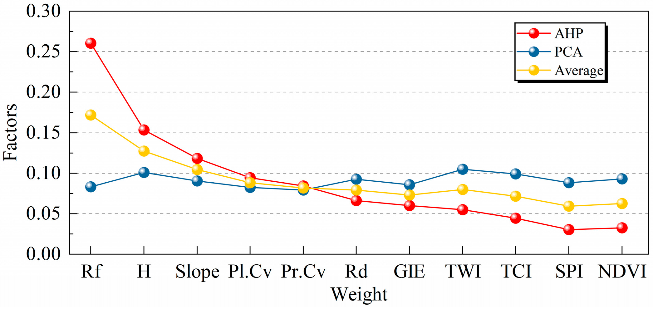
4.1. Calculation Results ofWeights
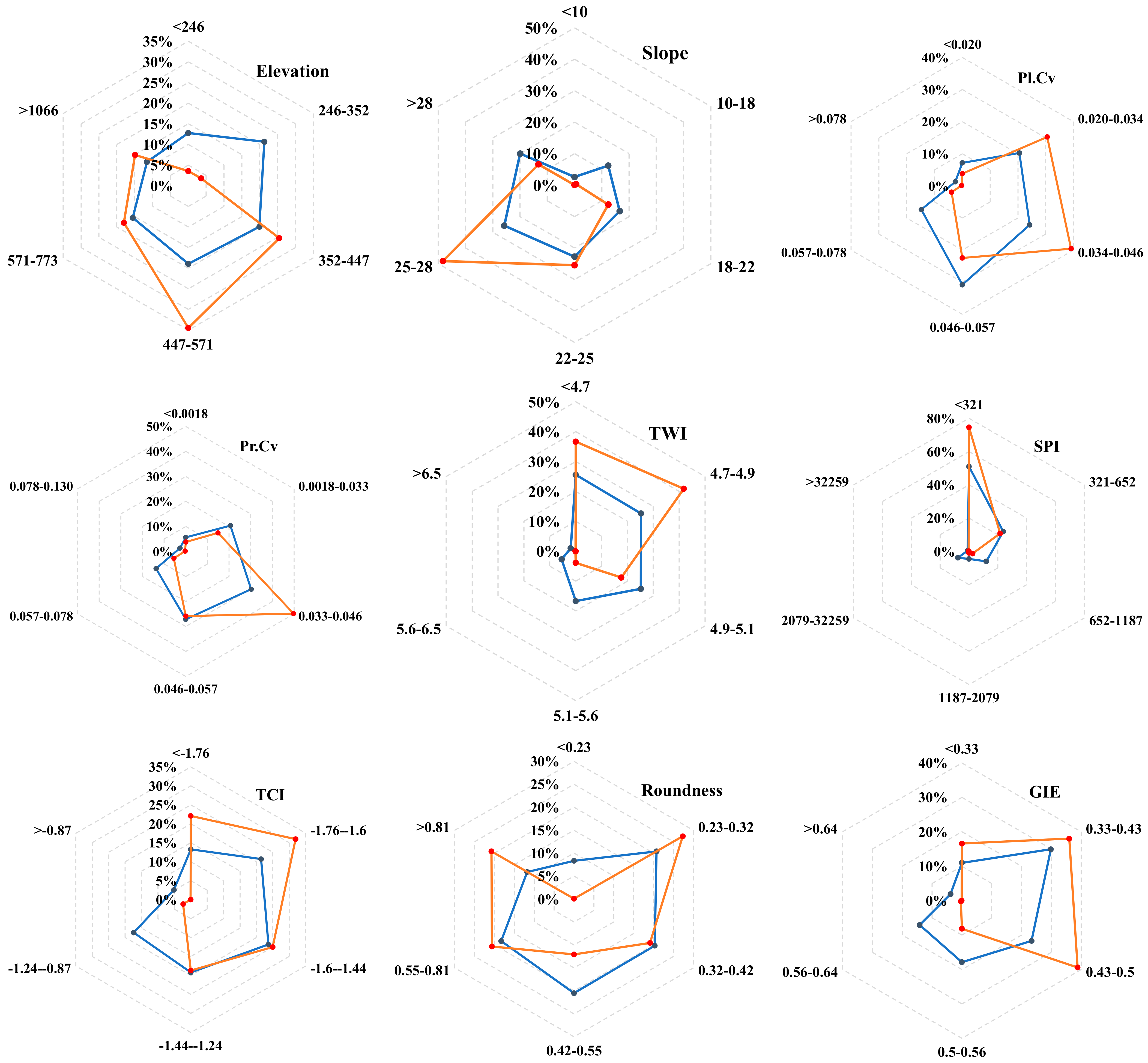
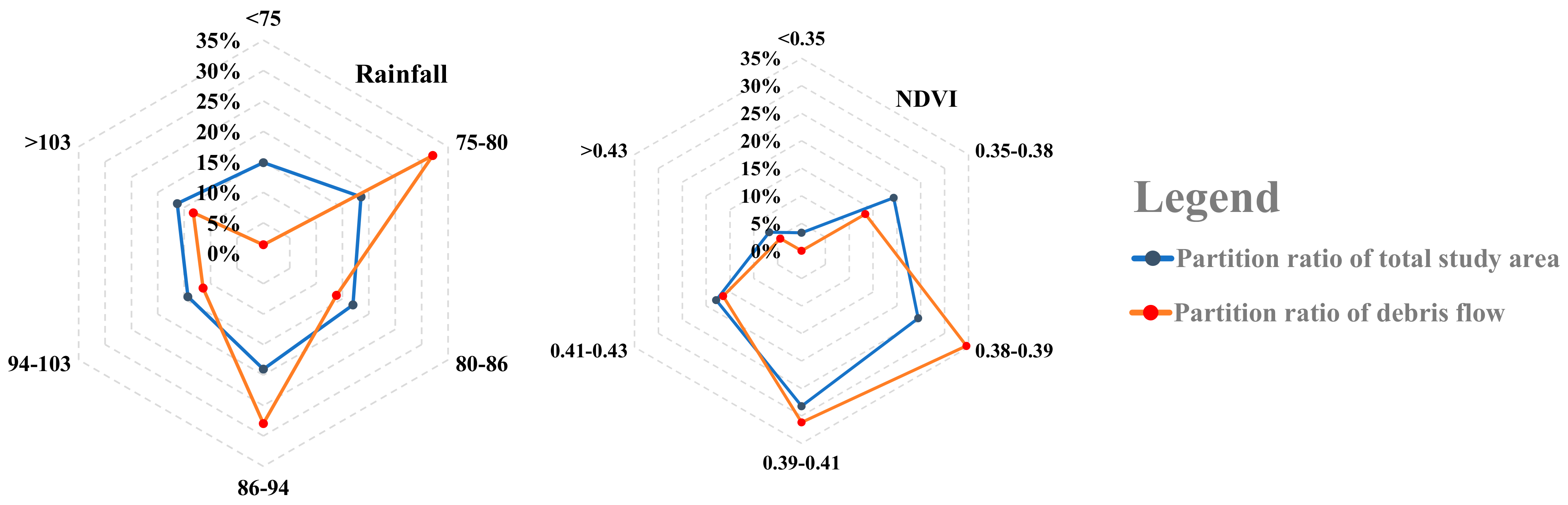
4.2. Distribution of Debris Flow in Different Classes of Factors
4.3. Correlation Analysis
5. Discussion
6. Conclusions
- 1.
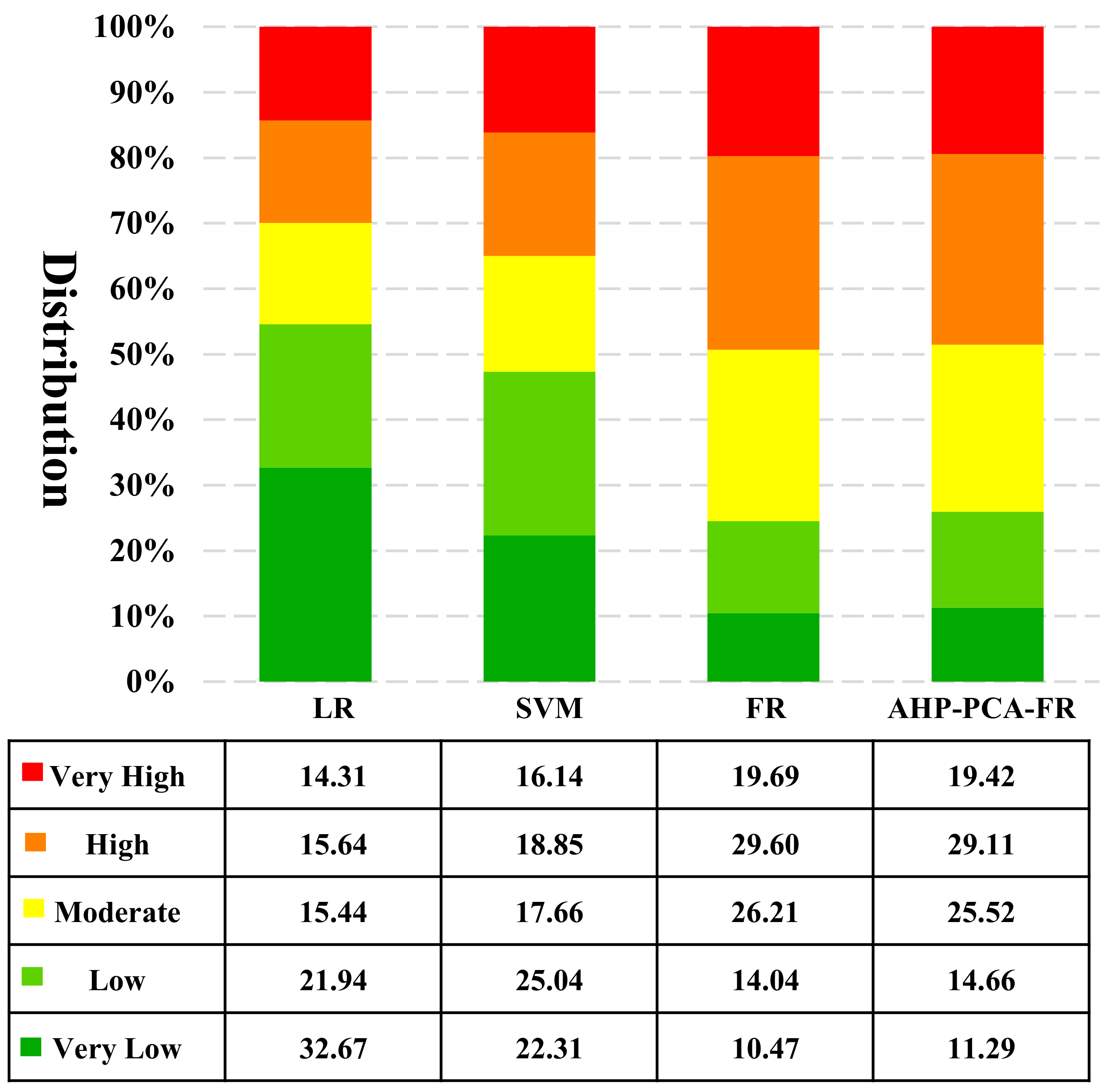
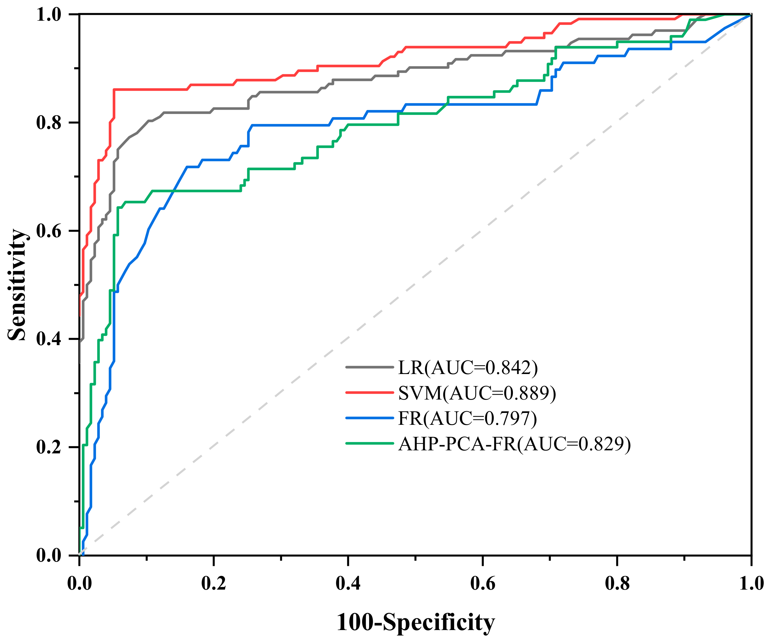
- Among the four models, the SVMmodel has the best performance and the highest prediction accuracy, with AUC = 0.889, followed by LR (AUC = 0.842), ACA–PCA–FR (AUC = 0.829) and FR (AUC = 0.797). The results show that SVM can still maintain very high prediction accuracy in the case of small sample data, learning can be strong and have a fast convergence, and has strong adaptability to high-dimensional samples, which is very suitable for the evaluation and analysis of geological disasters.
- 2.
- Among the four models, the results of the FR and ACA–PCA–FR models are relatively similar. These two methods are traditional weight evaluation methods. According to the field survey results and AUC values, the accuracy of these two methods is relatively low. The results of LR and SVM, as two widely-used machine learning algorithms, are similar, more consistent with the field survey results, and the AUC value is relatively high, so in this study, the machine learning algorithm is more accurate and reasonable.
Author Contributions
Funding
Institutional Review Board Statement
Informed Consent Statement
Data Availability Statement
Acknowledgments
Conflicts of Interest
Appendix A

| No. | H (m) | Slope (°) | Pl.Cv | Pr.Cv | TWI | SPI | TCI | Rd | GIE | Rf | NDVI |
|---|---|---|---|---|---|---|---|---|---|---|---|
| 1 | 243.65 | 20.13 | 0.04 | 0.18 | 5.04 | 51.76 | −1.55 | 0.42 | 0.66 | 85.36 | 0.41 |
| 2 | 505.38 | 25.92 | 0.05 | 0.04 | 4.63 | 219.43 | −1.78 | 0.37 | 0.42 | 89.65 | 0.38 |
| 3 | 1038.43 | 25.57 | 0.04 | 0.06 | 4.67 | 206.57 | −1.84 | 0.43 | 0.21 | 75.51 | 0.39 |
| 4 | 602.15 | 26.64 | 0.03 | 0.06 | 4.70 | 381.37 | −1.90 | 0.46 | 0.39 | 90.60 | 0.38 |
| 5 | 931.01 | 26.22 | 0.04 | 0.05 | 4.71 | 135.54 | −1.74 | 0.43 | 0.21 | 77.37 | 0.40 |
| 6 | 749.67 | 30.09 | 0.05 | 0.00 | 4.56 | 219.89 | −1.58 | 0.42 | 0.47 | 80.98 | 0.44 |
| 7 | 1008.40 | 25.66 | 0.01 | 0.01 | 4.84 | 273.88 | −1.46 | 0.43 | 0.21 | 77.23 | 0.41 |
| 8 | 967.57 | 27.50 | 0.03 | 0.06 | 4.77 | 286.41 | −1.65 | 0.41 | 0.31 | 80.01 | 0.41 |
| 9 | 869.67 | 26.78 | 0.03 | 0.06 | 4.72 | 156.73 | −1.74 | 0.45 | 0.52 | 80.43 | 0.41 |
| 10 | 784.33 | 26.03 | 0.00 | 0.04 | 4.48 | 80.38 | −2.18 | 0.45 | 0.53 | 80.58 | 0.41 |
| 11 | 437.44 | 24.66 | −0.02 | 0.09 | 4.81 | 119.62 | −2.06 | 0.56 | 0.47 | 87.57 | 0.46 |
| 12 | 269.94 | 28.29 | −0.01 | 0.08 | 4.52 | 148.31 | −2.30 | 0.68 | 0.46 | 79.67 | 0.48 |
| 13 | 263.18 | 27.44 | −0.06 | 0.04 | 4.54 | 153.34 | −2.46 | 0.43 | 0.45 | 79.76 | 0.48 |
| 14 | 418.28 | 27.99 | 0.06 | −0.01 | 4.54 | 309.73 | −1.56 | 0.38 | 0.36 | 78.21 | 0.44 |
| 15 | 738.46 | 26.25 | −0.02 | 0.09 | 4.70 | 160.45 | −2.17 | 0.63 | 0.19 | 75.40 | 0.46 |
| 16 | 820.86 | 27.17 | 0.04 | 0.02 | 4.64 | 187.79 | −1.68 | 0.63 | 0.19 | 76.35 | 0.41 |
| 17 | 546.49 | 27.14 | 0.00 | 0.00 | 4.54 | 123.96 | −1.85 | 0.39 | 0.36 | 74.29 | 0.46 |
| 18 | 392.30 | 27.96 | 0.01 | 0.07 | 4.72 | 295.73 | −1.97 | 0.46 | 0.35 | 78.19 | 0.43 |
| 19 | 307.44 | 28.72 | −0.02 | 0.07 | 4.49 | 171.67 | −2.53 | 0.68 | 0.46 | 79.39 | 0.46 |
| 20 | 630.33 | 27.45 | 0.03 | 0.06 | 4.70 | 213.02 | −1.87 | 0.50 | 0.25 | 88.02 | 0.42 |
| 21 | 388.86 | 26.87 | 0.02 | 0.09 | 4.68 | 174.03 | −1.96 | 0.43 | 0.39 | 83.89 | 0.43 |
| 22 | 565.62 | 29.21 | 0.02 | 0.01 | 4.64 | 568.68 | −2.01 | 0.55 | 0.25 | 70.20 | 0.35 |
| 23 | 473.61 | 27.67 | 0.04 | 0.06 | 4.74 | 265.07 | −1.73 | 0.56 | 0.25 | 85.87 | 0.38 |
| 24 | 532.11 | 31.21 | 0.02 | −0.01 | 4.64 | 196.51 | −1.52 | 0.41 | 0.16 | 82.79 | 0.42 |
| 25 | 389.12 | 23.22 | 0.05 | 0.06 | 4.73 | 163.41 | −1.84 | 0.59 | 0.25 | 83.82 | 0.42 |
| 26 | 432.29 | 23.28 | 0.05 | 0.05 | 4.88 | 249.88 | −1.75 | 0.57 | 0.33 | 82.15 | 0.40 |
| 27 | 598.21 | 26.25 | −0.04 | 0.01 | 4.69 | 97.54 | −1.89 | 0.45 | 0.29 | 92.20 | 0.36 |
| 28 | 532.19 | 27.01 | 0.04 | 0.08 | 4.72 | 246.06 | −1.84 | 0.36 | 0.33 | 80.85 | 0.41 |
| 29 | 397.58 | 29.74 | −0.13 | 0.14 | 4.47 | 137.77 | −3.18 | 0.45 | 0.36 | 91.34 | 0.40 |
| 30 | 564.05 | 29.76 | −0.11 | 0.05 | 4.42 | 108.60 | −2.72 | 0.45 | 0.29 | 92.24 | 0.34 |
| 31 | 411.35 | 25.69 | 0.03 | 0.07 | 4.77 | 320.24 | −1.93 | 0.55 | 0.32 | 94.10 | 0.38 |
| 32 | 525.73 | 25.93 | 0.07 | 0.08 | 4.70 | 140.00 | −1.75 | 0.45 | 0.29 | 89.90 | 0.41 |
| 33 | 410.43 | 15.58 | 0.07 | 0.04 | 5.21 | 81.75 | −1.08 | 0.54 | 0.34 | 106.72 | 0.41 |
| 34 | 404.58 | 13.64 | 0.08 | 0.12 | 5.39 | 138.10 | −1.26 | 0.48 | 0.34 | 106.59 | 0.41 |
| 35 | 461.08 | 25.49 | 0.02 | 0.11 | 4.70 | 123.40 | −2.14 | 0.52 | 0.30 | 102.13 | 0.40 |
| 36 | 508.76 | 26.66 | 0.03 | 0.06 | 4.66 | 261.97 | −1.91 | 0.60 | 0.19 | 102.29 | 0.39 |
| 37 | 453.55 | 23.81 | 0.02 | 0.04 | 4.97 | 223.28 | −1.41 | 0.72 | 0.38 | 109.66 | 0.37 |
| 38 | 655.98 | 28.49 | 0.00 | −0.02 | 4.67 | 222.83 | −1.62 | 0.55 | 0.25 | 70.36 | 0.36 |
| 39 | 379.86 | 23.35 | 0.06 | 0.13 | 4.82 | 148.32 | −1.74 | 0.55 | 0.34 | 108.49 | 0.40 |
| 40 | 387.34 | 20.13 | 0.06 | 0.05 | 4.99 | 117.33 | −1.16 | 0.58 | 0.38 | 105.98 | 0.41 |
| 41 | 470.47 | 24.17 | 0.01 | 0.07 | 4.80 | 162.16 | −1.93 | 0.69 | 0.36 | 102.31 | 0.40 |
| 42 | 411.80 | 24.66 | 0.02 | 0.03 | 5.03 | 319.65 | −1.32 | 0.62 | 0.30 | 90.49 | 0.39 |
| 43 | 413.66 | 20.88 | 0.01 | 0.11 | 4.91 | 68.87 | −1.87 | 0.70 | 0.32 | 98.69 | 0.43 |
References
- Chong, Y.; Chen, G.; Meng, X.; Yang, Y.; Shi, W.; Bian, S.; Zhang, Y.; Yue, D. Quantitative analysis of artificial dam failure effects ondebrisflows-A case study of theZhouqu′8.8′debrisflowin northwestern China. Sci. Total Environ. 2021, 792, 148439. [Google Scholar] [CrossRef] [PubMed]
- Zhang, S.; Zhang, L.M.; Chen, H.X. Relationships among three repeated large-scale debris flows at Pubugou Ravine in the Wenchuan earthquake zone. Can. Geotech. J. 2014, 51, 951–965. [Google Scholar] [CrossRef]
- Ma, C.; Deng, J.Y.; Wang, R. Analysis of the triggering conditions and erosion of a runoff-triggered debris flow in Miyun County, Beijing, China. Landslides 2018, 15, 2475–2485. [Google Scholar] [CrossRef]
- Dormann, C.F.; Elith, J.; Bacher, S.; Buchmann, C.; Carl, G.; Carré, G.; Marquéz, J.R.G.; Gruber, B.; Lafourcade, B.; Leitão, P.J.; et al. Collinearity: A review of methods to deal with it and a simulation study evaluating their performance. Ecography 2013, 36, 27–46. [Google Scholar] [CrossRef]
- Robert, H. Soil slumps and debris flows: Prediction and Protection. Bull. Assoc. Eng. Geol. 1981, 18, 17–28. [Google Scholar]
- Feizizadeh, B.; Roodposhti, M.S.; Blaschke, T.; Aryal, J. Comparing GIS-based support vector machine kernel functions for landslide susceptibility mapping. Arab. J. Geosci. 2017, 10, 1–13. [Google Scholar] [CrossRef]
- Devkota, K.C.; Regmi, A.D.; Pourghasemi, H.R.; Yoshida, K.; Pradhan, B.; Ryu, I.C.; Dhital, M.R.; Althuwaynee, O.F. Landslide susceptibility mapping using certainty factor, index of entropy and logistic regression models in GIS and their comparison at Mugling-Narayanghat road section in Nepal Himalaya. Nat. Hazards 2013, 65, 135–165. [Google Scholar] [CrossRef]
- Chen, X.; Chen, H.; You, Y.; Liu, J. Susceptibility assessment of debris flows using the analytic hierarchy process method-a case study in Subao river valley, China. J. Rock Mech. Geotech. Eng. 2015, 7, 404–410. [Google Scholar] [CrossRef]
- Xu, W.; Yu, W.; Jing, S.; Zhang, G.; Huang, J. Debris flow susceptibility assessment by GIS and information value model in a large-scale region, Sichuan Province (China). Nat. Hazards 2013, 65, 1379–1392. [Google Scholar] [CrossRef]
- Shi, M.Y.; Chen, J.P.; Song, Y.; Zhang, W.; Song, S.Y.; Zhang, X.D. Assessing debris flow susceptibility in Heshigten Banner, Inner Mongolia, China, using principal component analysis and an improved fuzzy C-means algorithm. Bull. Eng. Geol. Environ. 2016, 75, 909–922. [Google Scholar] [CrossRef]
- Lee, S.; Sambath, T. Landslide susceptibility mapping in the Damrei Romel area, Cambodia using frequency ratio and logistic regression models. Environ. Geol. 2006, 50, 847–855. [Google Scholar] [CrossRef]
- Li, Z.H.; Chen, J.P.; Tan, C.; Zhou, X.; Li, Y.C.; Han, M.X. Debris flow susceptibility assessment based on topo-hydrological factors at different unit scales: A case study of Mentougou district, Beijing. Environ. Earth Sci. 2021, 80, 365. [Google Scholar] [CrossRef]
- Li, Y.C.; Chen, J.P.; Tan, C.; Li, Y.; Gu, F.F.; Zhang, Y.W.; Mehmood, Q. Application of the borderline-SMOTE method in susceptibility assessments of debris flows in Pinggu District, Beijing, China. Nat. Hazards 2021, 105, 2499–2522. [Google Scholar] [CrossRef]
- Kang, S.H.; Lee, S.R. Debris flow susceptibility assessment based on an empirical approach in the central region of South Korea. Geomorphology 2018, 308, 1–12. [Google Scholar] [CrossRef]
- Liang, Z.; Wang, C.M.; Zhang, Z.M. A comparison of statistical and machine learning methods for debris flow susceptibility mapping. Stoch. Environ. Res. Risk A 2020, 34, 1887–1907. [Google Scholar] [CrossRef]
- Lin, G.F.; Chang, M.J.; Huang, Y.C.; Ho, J.Y. Assessment of susceptibility to rainfall induced landslides using improved self-organizing linear output map, support vector machine, and logistic regression. Eng. Geol. 2017, 224, 62–74. [Google Scholar] [CrossRef]
- Cao, C.; Zhang, W.; Chen, J.P.; Shan, B.; Song, S.Y.; Zhan, J.W. Quantitative estimation of debris flow source materials by integrating multi-source data: A case study. Eng. Geol. 2021, 291, 106222. [Google Scholar] [CrossRef]
- Sun, X.H.; Chen, J.P.; Bao, Y.D.; Han, X.D.; Zhan, J.W.; Peng, W. Landslide Susceptibility Mapping Using Logistic Regression Analysis along the Jinsha River and Its Tributaries Close to Derong and Deqin County, Southwestern China. ISPRS Int. J. Geo-Inf. 2018, 7, 438. [Google Scholar] [CrossRef]
- McSherry, D. Strategic induction of decision trees. Knowl. Based Syst. 1988, 12, 269–275. [Google Scholar] [CrossRef]
- Sun, X.H.; Chen, J.P.; Li, Y.R.; Rene, N.N. Landslide Susceptibility Mapping along a Rapidly Uplifting River Valley of the Upper Jinsha River, Southeastern Tibetan Plateau, China. Remote Sens. 2022, 14, 1730. [Google Scholar] [CrossRef]
- Qiu, C.C.; Su, L.J.; Zou, Q.; Geng, X.Y. A hybrid machine-learning model to map glacier-related debris flow susceptibility along Gyirong Zangbo watershed under the changing climate. Sci. Total Environ. 2022, 818, 151752. [Google Scholar] [CrossRef]
- Ke, X.; Basanta, R. Comparison of Different Machine Learning Methods for Debris Flow Susceptibility Mapping: A Case Study in the Sichuan Province, China. Remote Sens. 2020, 12, 295. [Google Scholar]
- Elkadiri, R.; Sultan, M.; Youssef, A.M.; Elbayoumi, T.; Chase, R.; Bulkhi, A.B.; Al-Katheeri, M.M. A remote sensing-based approach for debris-flow susceptibility assessment using artificial neural networks and logistic regression modeling. IEEE J. Sel. Top. Appl. Earth Obs. Remote Sens. 2014, 7, 4818–4835. [Google Scholar] [CrossRef]
- Ahmad, H.; Chen, N.S.; Rahman, M.; Islam, M.M.; Pourghasemi, H.R.; Hussain, S.F.; Habumugisha, J.M.; Liu, E.L.; Zheng, H.; Ni, H.Y.; et al. Geohazards Susceptibility Assessment along the Upper Indus Basin Using Four Machine Learning and Statistical Models. ISPRS Int.Geo-Inf. 2021, 10, 315. [Google Scholar] [CrossRef]
- Pal, S.C.; Chakrabortty, R.; Saha, A.; Bozchaloei, S.K.; Pham, Q.B.; Linh, N.T.T.; Anh, D.T.; Janizadeh, S.; Ahmadi, K. Evaluation of debris flow and landslide hazards using ensemble framework of Bayesian- and tree-based models. Bull. Eng. Geol. Environ. 2022, 81, 5. [Google Scholar] [CrossRef]
- Ciccarese, G.; Mulas, M.; Corsini, A. Combining spatial modelling andregionalization ofrainfall thresholds fordebris flows hazard map- ping in the Emilia-Romagna Apennines (Italy). Landslides 2021, 18, 3513–3529. [Google Scholar]
- Vianello, D.; Vagnon, F.; Bonetto, S.; Mosca, P. Debris flowsusceptibilitymapping using the Rock Engineering System (RES) method: A case study. Landslides 2022, 1–22. [Google Scholar] [CrossRef]
- Cao, J.; Zhang, Z.; Du, J.; Zhang, L.; Song, Y.; Sun, G. Multi-geohazards susceptibility mapping based on machine learning—A case study in Jiuzhaigou, China. Nat. Hazards 2020, 102, 851–871. [Google Scholar] [CrossRef]
- Ma, C.; Wang, Y.J.; Du, C.; Wang, Y.Q.; Li, Y.P. Variation in initiation condition of debris flow in the mountain regions surrounding Beijing. Geomorphology 2016, 273, 323–334. [Google Scholar] [CrossRef]
- Li, Y.; Chen, J.; Zhang, Y.; Song, S.; Han, X.; Ammar, M. Debris flow susceptibility assessment and runout prediction: A case study in Shiyang Gully, Beijing, China. Int J. Environ. Res. 2020, 14, 365–383. [Google Scholar] [CrossRef]
- Cheng, W.M.; Wang, N.; Zhao, M.; Zhao, S.M. Relative tectonics and debris flow hazards in the Beijing mountain area from DEM-derived geomorphic indices and drainage analysis. Geomorphology 2016, 257, 134–142. [Google Scholar] [CrossRef]
- Han, H.; Wang, W.Y.; Mao, B.H. Borderline-SMOTE: A new over-sampling method in imbalanced data sets learning. Lect. Notes Comput. Sci. 2005, 3644, 878–887. [Google Scholar]
- Qin, S.; Lv, J.; Cao, C.; Ma, Z.; Hu, X.; Liu, F.; Qiao, S.; Dou, Q. Mapping debris flow susceptibility based on watershed unit and grid cell unit: A comparison study. Geomat. Nat. Hazards Risk 2019, 10, 1648–1666. [Google Scholar] [CrossRef]
- Ayalew, L.; Yamagishi, H. The application of GIS-based logistic regression for landslide susceptibility mapping in the Kakuda-Yahiko Mountains, Central Japan. Geomorphology 2005, 65, 15–31. [Google Scholar] [CrossRef]
- Tiranti, D.; Cavalli, M.; Crema, S.; Zerbato, M.; Graziadei, M.; Barbero, S.; Cremonini, R.; Silvestro, C.; Bodrato, G.; Tresso, F. Semi-quantitative method for the assessment of debris supply from slopes to river in ungauged catchments. Sci. Total Environ. 2016, 554, 337–348. [Google Scholar] [CrossRef]
- Zhang, Y.; Ge, T.; Tian, W.; Liou, Y.-A. Debris flow susceptibility mapping using machine-learning techniques in Shigatse Area, China. Remote Sens. 2019, 11, 2801. [Google Scholar] [CrossRef]
- Yilmaz, I. Comparison of landslide susceptibility mapping methodologies for Koyulhisar, Turkey: Conditional probability, logistic regression, artificial neural networks, and support vector machine. Environ. Earth Sci. 2010, 61, 821–836. [Google Scholar] [CrossRef]
- Suthaharan, S. Support Vector Machine. In Machine Learning Models and Algorithms for Big Data Classification; Springer: Boston, MA, USA, 2016; pp. 207–235. [Google Scholar]
- Xu, C.; Dai, F.; Xu, X.; Lee, Y.H. GIS-based support vector machine modeling of earthquake-triggered landslide susceptibility in the Jianjiang River watershed, China. Geomorphology 2012, 145–146, 70–80. [Google Scholar] [CrossRef]
- Li, T.; Qiu, S.; Mao, S.X.; Bao, R.; Deng, H.B. Evaluating water resource accessibility in Southwest China. Water 2019, 11, 1708. [Google Scholar] [CrossRef]
- Wang, Q.; Guo, Y.; Li, W.; He, J.; Wu, Z. Predictive modeling of landslide hazards in Wen County, northwestern China based on information value, weights-of-evidence, and certainty factor. Geomat. Nat. Hazards Risk 2019, 10, 820–835. [Google Scholar] [CrossRef]
- Ballabio, C.; Sterlacchini, S. Support vector machines for landslide susceptibility mapping: The Staffora river basin case study, Italy. Math. Geosci. 2012, 44, 47–70. [Google Scholar] [CrossRef]
- Moore, I.D.; Grayson, R.; Ladson, A. Digital terrain modeling: A review of hydrological, geomorphological, and biological applications. Hydrol Process 1991, 5, 3–30. [Google Scholar] [CrossRef]
- Beven, K.J.; Kirkby, M.J. A physically based variable contributing area model of basin hydrology. Hydrol. Sci. Bull. 1979, 24, 43–69. [Google Scholar] [CrossRef]
- Wilson, J.P.; Gallant, J.C. Digital Terrain Analysis. In Terrain Analysis: Principles and Applications; Wilson, J.P., Gallant, J.C., Eds.; Wiley: New York, NY, USA, 2000; pp. 1–27. [Google Scholar]
- Park, S.J.; McSweeney, K.; Lowery, B. Identifcation of the spatial distribution of soils using a process-based terrain characterization. Geoderma 2001, 103, 249–272. [Google Scholar] [CrossRef]
- Tang, C.; Zhu, J.; Li, W.L. Rainfall-triggered debris flows following the Wenchuan earthquake. Bull. Eng. Geol. Environ. 2009, 68, 187–194. [Google Scholar] [CrossRef]
- Tehrany, M.S.; Pradhan, B.; Mansor, S.; Ahmad, N. Flood susceptibility assessment using GIS based support vector machine model with different kernel types. Catena 2015, 125, 91–101. [Google Scholar] [CrossRef]
- Saaty, T.L. Modeling unstructured decision problems—The theory of analytical hierarchies. Math. Comput. Simul. 1978, 20, 147–158. [Google Scholar] [CrossRef]
- Chen, W.; Wang, J.; Xie, X.; Hong, H.; Van Trung, N.; Bui, D.T.; Wang, G.; Li, X. Spatial prediction of landslide susceptibility using integrated frequency ratio with entropy and support vector machines by different kernel functions. Environ. Earth Sci. 2016, 75, 1344. [Google Scholar] [CrossRef]
- Sabokbar, H.F.; Roodposhti, M.S.; Tazik, E. Landslide susceptibility mapping using geographically-weighted principal component analysis. Geomorphology 2014, 226, 15–24. [Google Scholar] [CrossRef]
- Zhou, C.; Yin, K.; Cao, Y.; Ahmed, B. Application of time series analysis and PSO–SVM model in predicting the Bazimen landslide in the Three Gorges Reservoir, China. Eng. Geol. 2016, 204, 108–120. [Google Scholar] [CrossRef]
- Yilmaz, I. Landslide susceptibility mapping using frequency ratio, logistic regression, artificial neural networks and their comparison: A case study from Kat landslides (Tokat-Turkey). Comput. Geosci. 2009, 35, 1125–1138. [Google Scholar] [CrossRef]
- Zhang, X.; Wu, Y.; Zhai, E.; Ye, P. Coupling analysis of the heat-water dynamics and frozen depth in a seasonally frozen zone. J. Hydrol. 2021, 593, 125603. [Google Scholar] [CrossRef]
- Wu, X.; Ren, F.; Niu, R. Landslide susceptibility assessment using object mapping units, decision tree, and support vector machine models in the Three Gorges of China. Environ. Earth Sci. 2013, 71, 4725–4738. [Google Scholar] [CrossRef]
- Bui, D.T.; Tuan, T.A.; Hoang, N.D.; Thanh, N.Q.; Nguyen, D.B.; Van Liem, N.; Pradhan, B. Spatial prediction of rainfall-induced landslides for the Lao Cai area (Vietnam) using a hybrid intelligent approach of least squares support vector machines inference model and artificial bee colony optimization. Landslides 2016, 14, 447–458. [Google Scholar]
- Bui, D.T.; Pradhan, B.; Lofman, O.; Revhaug, I. Landslide susceptibility assessment in Vietnam using support vector machines, decision tree, and Naïve Bayes models. Math. Probl. Eng. 2012, 2012, 1–26. [Google Scholar]
- Zhang, X.; Zhai, E.; Wu, Y.; Sun, D.; Lu, Y. Theoretical and Numerical Analyses on Hydro–Thermal–Salt–Mechanical Interaction of Unsaturated Salinized Soil Subjected to Typical Unidirectional Freezing Process. Int. J. Geomech. 2021, 21, 04021104. [Google Scholar] [CrossRef]
- Pradhan, B. A comparative study on the predictive ability of the decision tree, support vector machine and neuro-fuzzy models in landslide susceptibility mapping using GIS. Comput. Geosci. 2013, 51, 350–365. [Google Scholar] [CrossRef]
- Umar, Z.; Pradhan, B.; Ahmad, A.; Jebur, M.N.; Tehrany, M.S. Earthquake induced landslide susceptibility mapping using an integrated ensemble frequency ratio and logistic regression models in West Sumatera Province, Indonesia. Catena 2014, 118, 124–135. [Google Scholar] [CrossRef]
- Bui, D.T.; Tuan, T.A.; Klempe, H.; Pradhan, B.; Revhaug, I. Spatial prediction models for shallow landslide hazards: A comparative assessment of the efficacy of support vector machines, artificial neural networks, kernel logistic regression, and logistic model tree. Landslides 2015, 13, 361–378. [Google Scholar]
- Pradhan, B.; Lee, S. Landslide susceptibility assessment and factor effect analysis: Backpropagation artificial neural networks and their comparison with frequency ratio and bivariate logistic regression modelling. Environ. Model. Softw. 2010, 25, 747–759. [Google Scholar] [CrossRef]
- Pham, B.T.; Bui, D.T.; Prakash, I.; Nguyen, L.H.; Dholakia, M.B. A comparative study of sequential minimal optimization-based support vector machines, vote feature intervals, and logistic regression in landslide susceptibility assessment using GIS. Environ. Earth Sci. 2017, 76, 371. [Google Scholar] [CrossRef]
- Zhang, X.; Ye, P.; Wu, Y. Enhanced technology for sewage sludge advanced dewatering from an engineering practice perspective: A review. J. Environ. Manag. 2022, 321, 115938. [Google Scholar] [CrossRef] [PubMed]
- Meng, Q.; Miao, F.; Zhen, J.; Wang, X.; Wang, A.; Peng, Y.; Fan, Q. GIS-based landslide susceptibility mapping with logistic regression, analytical hierarchy process, and combined fuzzy and support vector machine methods: A case study from Wolong Giant Panda Natural Reserve, China. Bull. Eng. Geol. Environ. 2015, 75, 923–944. [Google Scholar] [CrossRef]
- Marjanović, M.; Kovačević, M.; Bajat, B.; Voženílek, V. Landslide susceptibility assessment using SVM machine learning algorithm. Eng. Geol. 2011, 123, 225–234. [Google Scholar] [CrossRef]
- Mather, P.M. The use of backpropagating artificial neural networks in land cover classification. Int. J. Remote Sens. 2003, 24, 4907–4938. [Google Scholar]
- Li, L.; Lan, H.; Guo, C.; Zhang, Y.; Li, Q.; Wu, Y. A modified frequency ratio method for landslide susceptibility assessment. Landslides 2017, 14, 727–741. [Google Scholar] [CrossRef]
- Kavzoglu, T.; Sahin, E.K.; Colkesen, I. Landslide susceptibility mapping using GIS-based multi-criteria decision analysis, support vector machines, and logistic regression. Landslides 2013, 11, 425–439. [Google Scholar] [CrossRef]


| n | 1 | 2 | 3 | 4 | 5 | 6 | 7 | 8 | 9 | 10 | 11 |
|---|---|---|---|---|---|---|---|---|---|---|---|
| RI | 0 | 0 | 0.58 | 0.90 | 1.12 | 1.24 | 1.32 | 1.41 | 1.45 | 1.49 | 1.51 |
| Factors | X1 | X2 | X3 | X4 | X5 | X6 | X7 | X8 | X9 | X10 | X11 | Weight |
|---|---|---|---|---|---|---|---|---|---|---|---|---|
| X1 | 1 | 2 | 3 | 4 | 4 | 5 | 6 | 5 | 6 | 7 | 3 | 0.260 |
| X2 | 1/2 | 1 | 2 | 3 | 3 | 4 | 2 | 2 | 3 | 3 | 3 | 0.154 |
| X3 | 1/3 | 1/2 | 1 | 2 | 2 | 3 | 2 | 3 | 3 | 4 | 2 | 0.118 |
| X4 | 1/4 | 1/3 | 1/2 | 1 | 2 | 2 | 3 | 2 | 3 | 2 | 3 | 0.095 |
| X5 | 1/4 | 1/3 | 1/2 | 1/2 | 1 | 2 | 3 | 3 | 2 | 3 | 2 | 0.084 |
| X6 | 1/5 | 1/4 | 1/3 | 1/2 | 1/2 | 1 | 2 | 2 | 3 | 2 | 3 | 0.066 |
| X7 | 1/6 | 1/2 | 1/2 | 1/3 | 1/3 | 1/2 | 1 | 2 | 3 | 3 | 2 | 0.060 |
| X8 | 1/5 | 1/2 | 1/3 | 1/2 | 1/3 | 1/2 | 1/2 | 1 | 2 | 3 | 4 | 0.055 |
| X9 | 1/6 | 1/3 | 1/3 | 1/3 | 1/2 | 1/3 | 1/3 | 1/2 | 1 | 4 | 3 | 0.044 |
| X10 | 1/7 | 1/3 | 1/4 | 1/2 | 1/3 | 1/2 | 1/3 | 1/3 | 1/4 | 1 | 2 | 0.031 |
| X11 | 1/3 | 1/3 | 1/2 | 1/3 | 1/2 | 1/3 | 1/2 | 1/4 | 1/3 | 1/2 | 1 | 0.033 |
| Factors | Weight | ||
|---|---|---|---|
| AHP | PCA | Average | |
| Rf | 0.260 | 0.083 | 0.172 |
| H | 0.154 | 0.101 | 0.127 |
| Slope | 0.118 | 0.091 | 0.104 |
| Pl.Cv | 0.095 | 0.082 | 0.088 |
| Pr.Cv | 0.084 | 0.079 | 0.082 |
| Rd | 0.066 | 0.092 | 0.079 |
| GIE | 0.060 | 0.086 | 0.073 |
| TWI | 0.055 | 0.105 | 0.080 |
| TCI | 0.044 | 0.099 | 0.072 |
| SPI | 0.031 | 0.088 | 0.059 |
| NDVI | 0.033 | 0.093 | 0.063 |
| Factor | Class | Study Area | Debris Flows Area | FR | ||
|---|---|---|---|---|---|---|
| Count | Ratio (%) | Count | Ratio (%) | |||
| Elevation (m) | <246 | 1,763,582 | 12.77 | 32,373 | 3.54 | 0.278 |
| 246–352 | 2,943,221 | 21.30 | 32,857 | 3.60 | 0.169 | |
| 352–447 | 2,749,383 | 19.90 | 232,606 | 25.47 | 1.280 | |
| 447–571 | 2,615,987 | 18.94 | 314,927 | 34.48 | 1.821 | |
| 571–773 | 2,147,022 | 15.54 | 164,597 | 18.02 | 1.160 | |
| >1066 | 1,596,180 | 11.55 | 136,007 | 14.89 | 1.289 | |
| Slope (°) | <10 | 355,183 | 2.57 | 328 | 0.04 | 0.014 |
| 10–18 | 1,706,124 | 12.35 | 5503 | 0.60 | 0.049 | |
| 18–22 | 2,289,905 | 16.58 | 113,069 | 12.38 | 0.747 | |
| 22–25 | 3,142,477 | 22.75 | 232,494 | 25.45 | 1.119 | |
| 25–28 | 3,564,604 | 25.80 | 441,176 | 48.30 | 1.872 | |
| >28 | 2,757,082 | 19.96 | 120,797 | 13.23 | 0.663 | |
| Pl.Cv | <0.020 | 989,053 | 7.16 | 34,787 | 3.81 | 0.532 |
| 0.020–0.034 | 2,834,110 | 20.51 | 278,744 | 30.52 | 1.488 | |
| 0.034–0.046 | 3,350,592 | 24.25 | 357,437 | 39.13 | 1.614 | |
| 0.046–0.057 | 4,254,670 | 30.80 | 204,989 | 22.44 | 0.729 | |
| 0.057–0.078 | 2,036,610 | 14.74 | 35,319 | 3.87 | 0.262 | |
| >0.078 | 350,340 | 2.54 | 2091 | 0.23 | 0.090 | |
| Pr.Cv | <0.0018 | 776,090 | 5.62 | 34,546 | 3.78 | 0.673 |
| 0.0018–0.033 | 2,850,849 | 20.64 | 135,740 | 14.86 | 0.720 | |
| 0.033–0.046 | 4,174,347 | 30.22 | 454,510 | 49.76 | 1.647 | |
| 0.046–0.057 | 3,751,047 | 27.15 | 235,962 | 25.83 | 0.951 | |
| 0.057–0.078 | 1,892,812 | 13.70 | 50,186 | 5.49 | 0.401 | |
| >0.078 | 370,230 | 2.68 | 2423 | 0.27 | 0.099 | |
| TWI | <4.7 | 3,530,258 | 25.55 | 334,721 | 36.65 | 1.434 |
| 4.7–4.9 | 3,486,820 | 25.24 | 381,479 | 41.77 | 1.655 | |
| 4.9–5.1 | 3,477,971 | 25.17 | 161,005 | 17.63 | 0.700 | |
| 5.1–5.6 | 2,304,522 | 16.68 | 35,393 | 3.88 | 0.232 | |
| 5.6–6.5 | 748,518 | 5.42 | 441 | 0.05 | 0.009 | |
| >6.5 | 267,286 | 1.93 | 326 | 0.04 | 0.018 | |
| SPI | <321 | 7,044,594 | 50.99 | 681,341 | 74.6 | 1.463 |
| 321–652 | 3,294,696 | 23.85 | 197,750 | 21.65 | 0.908 | |
| 652–1187 | 1,661,894 | 12.03 | 23,440 | 2.57 | 0.213 | |
| 1187–2079 | 626,998 | 4.54 | 8392 | 0.92 | 0.202 | |
| 2079–32,259 | 1,063,258 | 7.70 | 353 | 0.04 | 0.005 | |
| >32,259 | 123,935 | 0.90 | 2091 | 0.23 | 0.255 | |
| TCI | <−1.76 | 1,830,826 | 13.25 | 201,634 | 22.08 | 1.666 |
| −1.76–1.6 | 2,956,309 | 21.40 | 291,421 | 31.91 | 1.491 | |
| −1.6–1.44 | 3,267,552 | 23.65 | 228,035 | 24.97 | 1.056 | |
| −1.44–1.24 | 2,652,379 | 19.20 | 170,634 | 18.68 | 0.973 | |
| −1.24–0.87 | 2,401,896 | 17.39 | 21,315 | 2.33 | 0.134 | |
| >−0.87 | 706,413 | 5.11 | 328 | 0.04 | 0.007 | |
| Roundness | <0.23 | 1,149,635 | 8.32 | 576 | 0.06 | 0.008 |
| 0.23–0.32 | 2,869,935 | 20.77 | 249,892 | 27.36 | 1.317 | |
| 0.32–0.42 | 2,807,727 | 20.32 | 174,583 | 19.11 | 0.941 | |
| 0.42–0.55 | 2,830,499 | 20.49 | 110,037 | 12.05 | 0.588 | |
| 0.55–0.81 | 2,530,300 | 18.32 | 188,650 | 20.65 | 1.128 | |
| >0.81 | 1,627,279 | 11.78 | 189,629 | 20.76 | 1.763 | |
| GIE | <0.33 | 1,518,871 | 10.99 | 151,473 | 16.58 | 1.508 |
| 0.33–0.43 | 4,122,934 | 29.84 | 328,981 | 36.02 | 1.207 | |
| 0.43–0.5 | 3,229,952 | 23.38 | 354,525 | 38.82 | 1.660 | |
| 0.5–0.56 | 2,467,237 | 17.86 | 74,420 | 8.15 | 0.456 | |
| 0.56–0.64 | 1,953,781 | 14.14 | 3199 | 0.35 | 0.025 | |
| >0.64 | 522,600 | 3.78 | 769 | 0.08 | 0.022 | |
| Rainfall (mm) | <74.5 | 2,053,685 | 14.87 | 12,687 | 1.39 | 0.093 |
| 74.5–80.4 | 2,559,075 | 18.52 | 293,259 | 32.11 | 1.733 | |
| 80.4–86.1 | 2,344,335 | 16.97 | 126,493 | 13.85 | 0.816 | |
| 86.1–94.2 | 2,629,605 | 19.03 | 255,501 | 27.97 | 1.470 | |
| 94.2–103.4 | 1,974,843 | 14.29 | 104,323 | 11.42 | 0.799 | |
| >103.4 | 2,253,822 | 16.31 | 121,104 | 13.26 | 0.813 | |
| NDVI | <0.35 | 454,500 | 3.29 | 0 | 0 | 0.000 |
| 0.35–0.38 | 2,669,162 | 19.32 | 122,156 | 13.37 | 0.692 | |
| 0.38–0.39 | 3,380,910 | 24.47 | 315,819 | 34.58 | 1.413 | |
| 0.39–0.41 | 3,899,555 | 28.23 | 284,587 | 31.16 | 1.104 | |
| 0.41–0.43 | 2,474,058 | 17.91 | 150,116 | 16.44 | 0.918 | |
| >0.43 | 937,190 | 6.78 | 40,689 | 4.45 | 0.657 | |
| Factors | GIE | H | NDVI | Pl.Cv | Pr.Cv | Slope | Rf | SPI | TCI | TWI | Rd |
|---|---|---|---|---|---|---|---|---|---|---|---|
| GIE | 1.000 | −0.550 | −0.317 | 0.199 | 0.188 | −0.727 | 0.191 | 0.166 | 0.658 | 0.696 | −0.257 |
| H | −0.550 | 1.000 | 0.155 | −0.170 | −0.139 | 0.603 | −0.535 | −0.115 | −0.488 | −0.524 | 0.210 |
| NDVI | −0.317 | 0.155 | 1.000 | −0.029 | −0.041 | 0.378 | −0.277 | −0.116 | −0.383 | −0.432 | 0.116 |
| Pl.Cv | 0.199 | −0.170 | −0.029 | 1.000 | 0.980 | −0.112 | 0.133 | 0.277 | −0.019 | −0.040 | −0.032 |
| Pr.Cv | 0.188 | −0.139 | −0.041 | 0.980 | 1.000 | −0.089 | 0.105 | 0.311 | −0.046 | −0.056 | −0.024 |
| Slope | −0.727 | 0.603 | 0.378 | −0.112 | −0.089 | 1.000 | −0.299 | −0.005 | −0.821 | −0.904 | 0.388 |
| Rf | 0.191 | −0.535 | −0.277 | 0.133 | 0.105 | −0.299 | 1.000 | −0.143 | 0.183 | 0.130 | −0.041 |
| SPI | 0.166 | −0.115 | −0.116 | 0.277 | 0.311 | −0.005 | −0.143 | 1.000 | 0.078 | 0.132 | −0.021 |
| TCI | 0.658 | −0.488 | −0.383 | −0.019 | −0.046 | −0.821 | 0.183 | 0.078 | 1.000 | 0.923 | −0.300 |
| TWI | 0.696 | −0.524 | −0.432 | −0.040 | −0.056 | −0.904 | 0.130 | 0.132 | 0.923 | 1.000 | −0.362 |
| Rd | −0.257 | 0.210 | 0.116 | −0.032 | −0.024 | 0.388 | −0.041 | −0.021 | −0.300 | −0.362 | 1.000 |
Disclaimer/Publisher’s Note: The statements, opinions and data contained in all publications are solely those of the individual author(s) and contributor(s) and not of MDPI and/or the editor(s). MDPI and/or the editor(s) disclaim responsibility for any injury to people or property resulting from any ideas, methods, instructions or products referred to in the content. |
© 2023 by the authors. Licensee MDPI, Basel, Switzerland. This article is an open access article distributed under the terms and conditions of the Creative Commons Attribution (CC BY) license (https://creativecommons.org/licenses/by/4.0/).
Share and Cite
Gu, F.; Chen, J.; Sun, X.; Li, Y.; Zhang, Y.; Wang, Q. Comparison of Machine Learning and Traditional Statistical Methods in Debris Flow Susceptibility Assessment: A Case Study of Changping District, Beijing. Water 2023, 15, 705. https://doi.org/10.3390/w15040705
Gu F, Chen J, Sun X, Li Y, Zhang Y, Wang Q. Comparison of Machine Learning and Traditional Statistical Methods in Debris Flow Susceptibility Assessment: A Case Study of Changping District, Beijing. Water. 2023; 15(4):705. https://doi.org/10.3390/w15040705
Chicago/Turabian StyleGu, Feifan, Jianping Chen, Xiaohui Sun, Yongchao Li, Yiwei Zhang, and Qing Wang. 2023. "Comparison of Machine Learning and Traditional Statistical Methods in Debris Flow Susceptibility Assessment: A Case Study of Changping District, Beijing" Water 15, no. 4: 705. https://doi.org/10.3390/w15040705