Predicting Influent and Effluent Quality Parameters for a UASB-Based Wastewater Treatment Plant in Asia Covering Data Variations during COVID-19: A Machine Learning Approach

Abstract

A region’s population growth inevitably results in higher water consumption. This persistent rise in water use increases the region’s wastewater production. Consequently, due to this increase in wastewater (influent), Wastewater Treatment Plants (WWTPs) are required to run effectively in order to handle the huge demand for treated/processed water (effluent). Knowing in advance the influent and effluent parameters increases the operational efficiency and enables cost-effective utilization of diverse resources at wastewater treatment plants. This paper is based on a prediction/forecasting of an influent quality parameter, namely total MLD, as well as effluent quality parameters, namely MPN, BOD, DO, COD and pH for the real-time data collected pre-, during and post-COVID-19 at the Bharwara WWTP in Lucknow, India. It is the largest UASB-based wastewater treatment facility in Uttar Pradesh and the second largest in Asia. In this paper, we propose a novel model namely, wPred comprising extensions of SARIMA with seasonal order and ANN-based ML models to estimate the influent and effluent quality parameters, respectively, and compare it with the existing machine learning models. The lowest sMAPE error for the influent parameters using wPred is 2.59%. The findings of the paper show a strong correlation (R-value), up to 0.99, between the effluent parameters actually measured and predicted. As a result, the model designed in this paper has an acceptable level of accuracy and generalizability which efficiently predicts/forecasts the performance of Bharwara WWTP.

1. Introduction

Water is one of the most important natural resources for all life on Earth. It has always been important to consider the availability and quality of water when selecting not only where people will live but also how joyful those lives will be. India’s entire usable water supply, which has been calculated to be around 1124 Billion Cubic Metres (BCM), is just 28% of the water generated through precipitation (692 BCM from surface and 435 BCM from ground) [1]. Approximately 87% (689 BCM) of water use is diverted for irrigation, and by 2050, that percentage may rise to 1072 BCM. Groundwater is a significant irrigation supply [2].

1.1. Utilization of Water in Various Sectors

Fresh water is used commercially for establishments including hotels, restaurants, offices, motels, other commercial buildings, and both civilian and military institutions. The majority of people’s daily water use is primarily for domestic purposes. Water used for daily household chores, including drinking, eating, cooking, cleaning, bathing, laundry, washing dishes and watering lawns and landscapes, is referred to as domestic use [3].

The nation’s businesses use industrial water as a crucial resource for things such as processing, sanitation, conveyance, attenuation and cooling in manufacturing plants. Chemical, steel and petroleum refining are a few of the major water-consuming sectors [1]. The same water is frequently used by industries multiple times for different reasons.

Water for irrigation is the water that is used for agricultural, vineyard, pasture, and horticultural crops. It is also used to irrigate pastures, prevent frost and freezing damage, apply chemicals, cool crops, harvest them and remove salts from the root zone of crops. The extraction of natural deposits, substances such as anthracite coal and mineral products, solvents such as crude oil and gases such as natural energy resources all include using water. As a subset of mining activity, this category comprises quarrying, milling (including trouncing, screenings, washing and flotation) and other processes. About 34% of the water utilized for mining is saline, which is a sizable percentage [3].

1.2. Categorization of Wastewater

With utilization of water in various domains as discussed above, wastewater is also produced. The categorization of wastewater is given below:

• Human excreta (faeces and urine), which is frequently combined with old toilet paper or wipes, can be the source of wastewater. If this waste is collected by flushing toilets, it is referred to as “blackwater” [4].
• Washing water (for one’s own clothing, dishes, floors, and other items), commonly referred to as greywater or sullage.
• Excess domestically produced liquids (drinks, cooking leftovers, insecticides, lubrication oil, paint, cleaning agents, etc.).
• Urban rainwater runoff from roads, parking lots, roofs, walkways and pavements (contains lubricants, animal droppings, garbage, gasoline or diesel, rubber remnants from tyres, soap scum, metals from vehicle exhausts, etc.).
• Highway runoff, including lubricants, anti-icing chemicals and rubber remnants, notably from tyres, and storm sewers (trash included) [5].
• Liquids made by humans (pesticides dumped illegally, used oils, etc.).
• Agriculture discharge (pesticides and other chemicals get mixed with the water).
• Carbon discharge from the coal and oil industry and their byproducts.
• Industrial plant discharge (loam, sand, alkali and chemical byproducts) and industrial waste, etc.) [6].

As the wastewater is produced, it is processed at Wastewater Treatment Plants (WWTPs) that remove numerous particles and chemicals that are hazardous [7]. As a result, WWTPs play a significant role in influencing both urban and rural settings. Growth in a region’s population causes a rise in water consumption, and a continual rise in water use leads to an increase in the amount of wastewater the area produces [8]. In order to satisfy the demand for effluent (processed) water, the wastewater treatment plants must work effectively [5,9]. Their operational efficiency is enabled by cost- effective utilization of diverse resources which can be ensured by knowing in advance the quality parameters of the wastewater entering (influent) the WWTP and processed/treated water (effluent) leaving the WWTP.

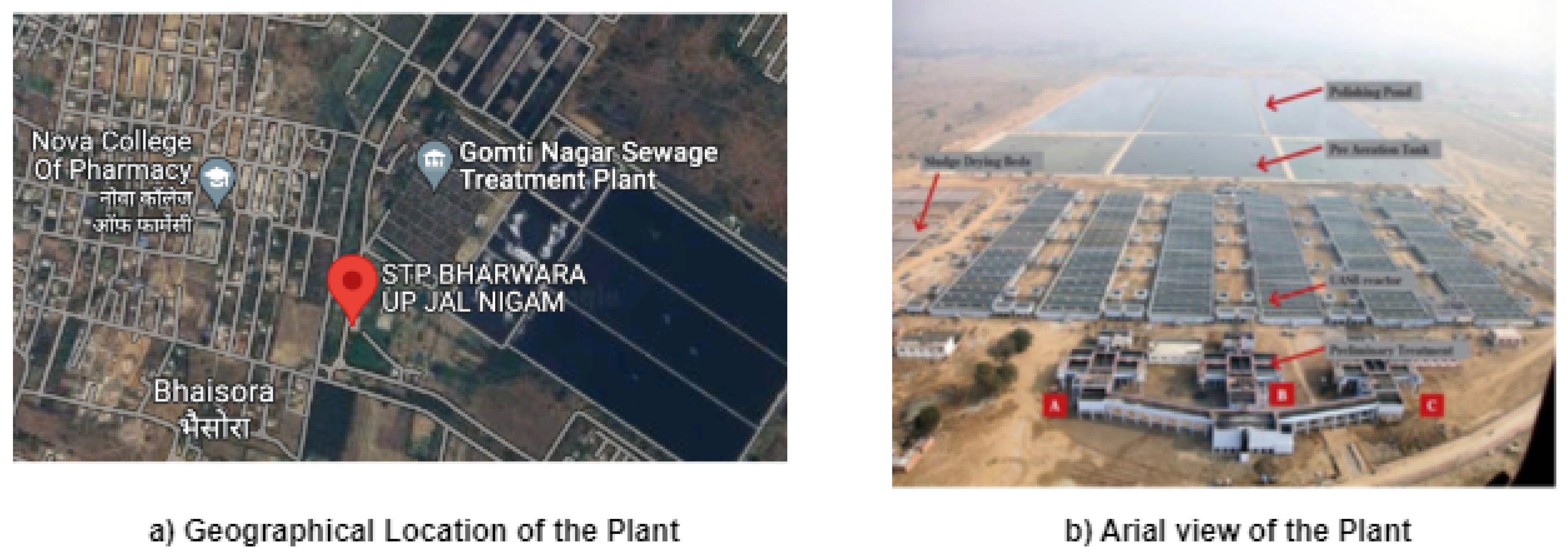
In this paper, we predict influent and effluent quality parameters of one of the largest UASB-based Wastewater Treatment Plants in Uttar Pradesh and the second largest in Asia, namely the Bharwara Wastewater Treatment Plant. A brief description of the plant is given below.

1.3. Bharwara Wastewater Treatment Plant

The Bharwara Wastewater Treatment Plant (WWTP) situated in Lucknow, as shown in Figure 1, is the second largest UASB-based wastewater treatment plant in Asia and can operate and process 345 MLD (million litres per day) on average with the capacity to handle a peak load of 517 MLD of sewage, which is processed from three different inlet chambers: A, B and C as shown in the Figure 1. A detailed description of the plant is presented in [10].

Bharwara WWTP has five zones, namely preliminary treatment, UASB reactor, polishing pond, pre-aeration tank and sludge drying beds as shown in Figure 1. Different parameters of water quality were recorded from the inlet chamber, the outlet of the UASB reactor, the polishing pond, the outlet of chlorine contact tank and the primary sludge as shown in

Table 1. Locations and measuring parameters [10].

Location	Parameters
Inlet Chamber	pH, BOD, Temperature, TSS, flow, COD, Phosphorous, oil and DO
Outlet of UASB Reactor	BOD, pH, Suspended Solids, COD
Polishing Pond	Dissolved Oxygen, pH
Outlet of Chlorine Contact Tank	BOD, pH, Suspended solids, COD, Residual Chlorine, Fecal Coliform, Dissolved Oxygen.
Primary Sludge	pH, Volatile solids, Total Solids.

. Table 1 presents the location as well as the parameters of each zone of the plant.

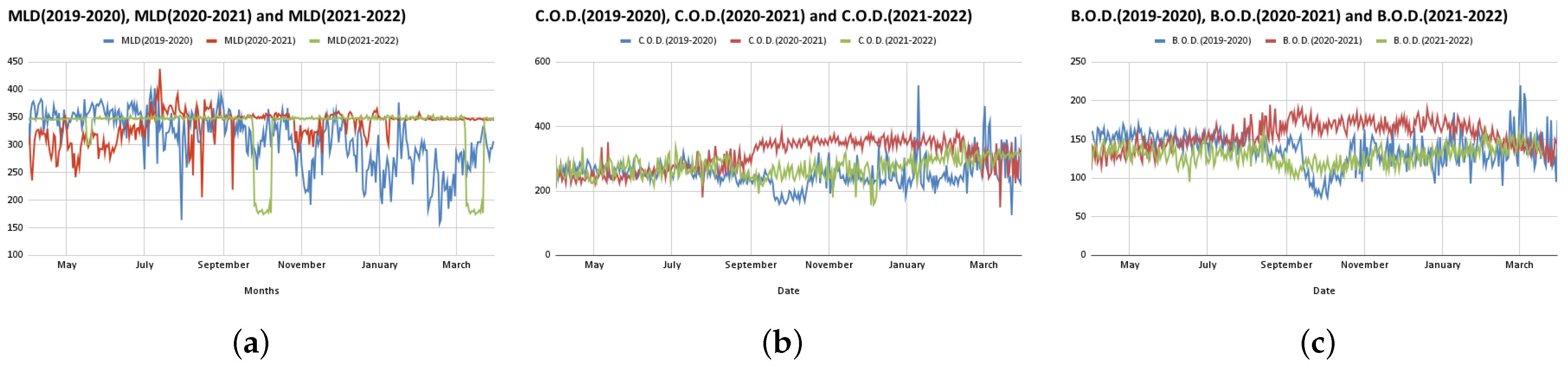
In this paper, we analyze the flow of influent as well as the quality parameters of effluent, namely pH value (pH), dissolved oxygen (DO), chemical oxygen demand (COD), total suspended solids (TSSs), biochemical oxygen demand (BOD) and myeloproliferative neoplasms (MPN) at the Bharwara WWTP and propose a novel model to predict these quality parameters of influent and effluent. The range and units of these parameters are shown in

Table 2. Influent and effluent quality parameter range [10].

Data Parameters	Units	Range (Influent)	Range (Effluent)
pH	No.	6–8	7–9
DO	mg/L	0	$>4$
TSS	mg/L	300–600	$<50$
COD	mg/L	200–500	$<100$
BOD	mg/L	150–250	$<30$
MPN	No./100 mL	106–109	106–109
Flow Rate	Millions of Litre per Day	250–400

.

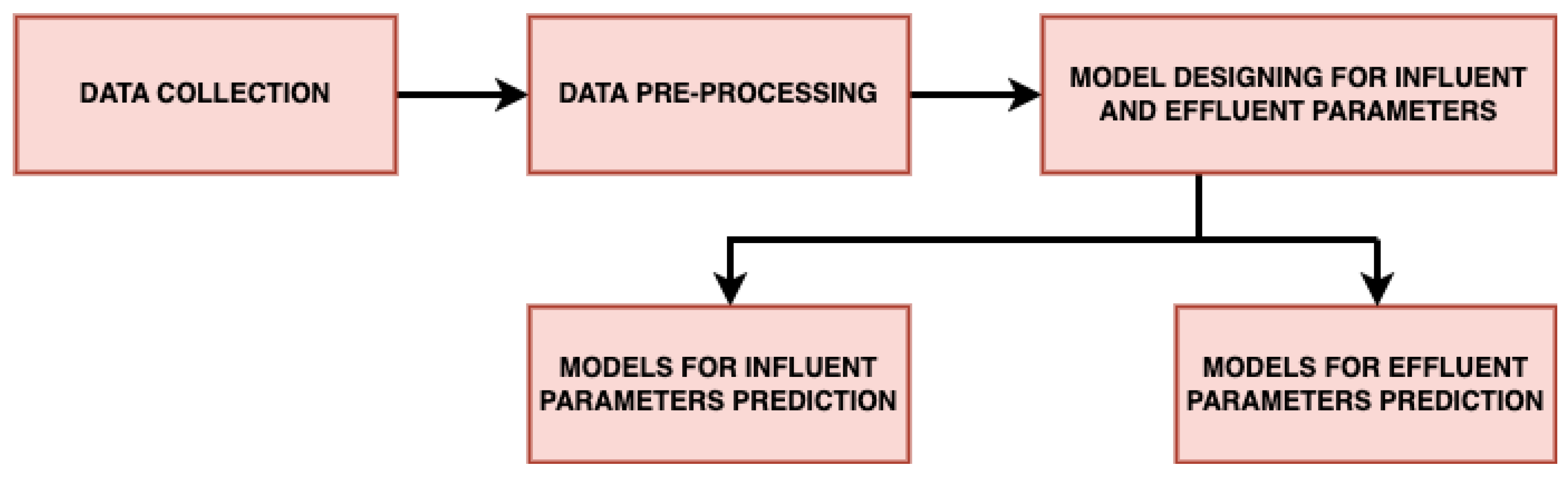
The novelty of this paper is to propose and implement a machine-learning-based model named wPred to predict influent and effluent quality parameters. The proposed model provides centralized monitoring of WWTP operations and processes. By understanding the influent and effluent quality parameters in advance, the model proposed in this paper enables cost-effective utilization of various resources at wastewater treatment plants. Another highlight of the paper is that in the proposed novel model we have collected real-time data which are taken from the various locations at the plant and trained the model using the data. These locations and parameters are given in Table 1. The total duration of the data collected for analysis purposes was from April 2019 to May 2022—a total of 38 months pre-, during and post-COVID-19 [10].

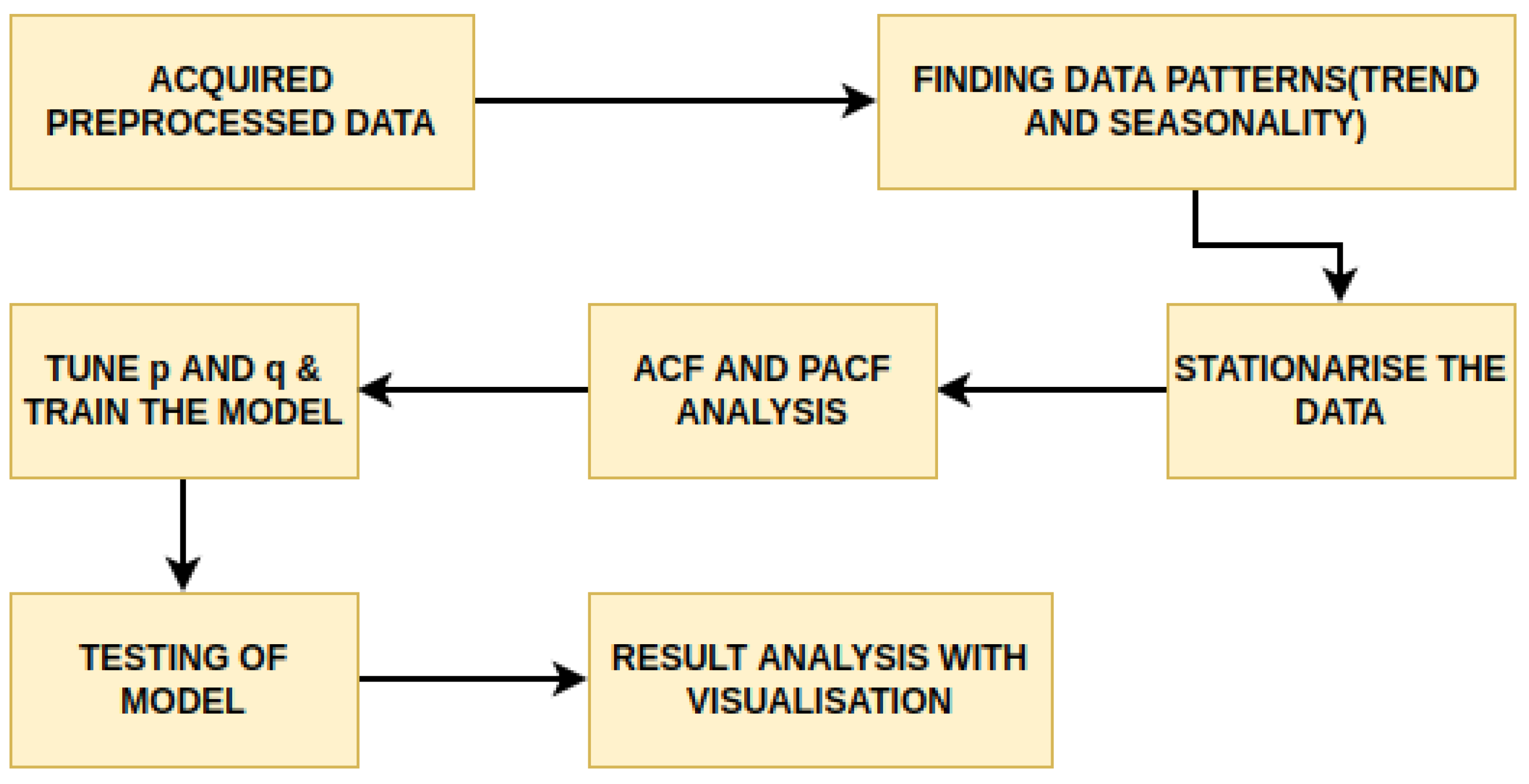
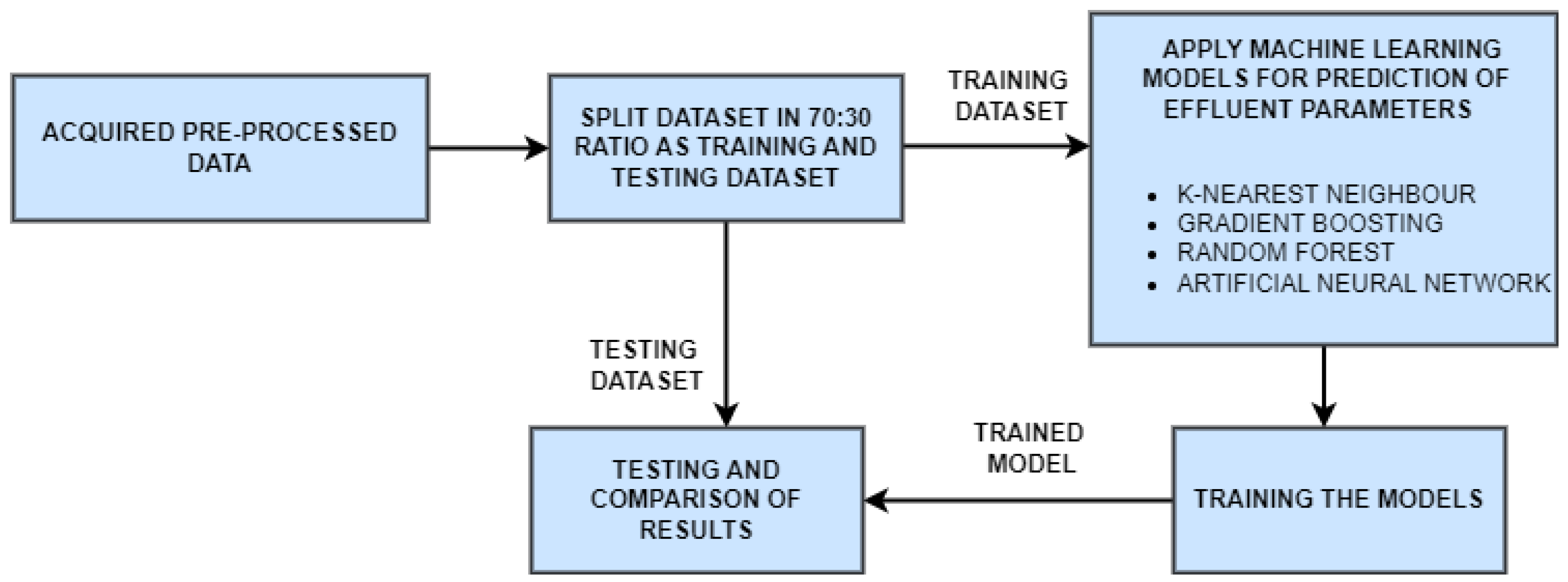
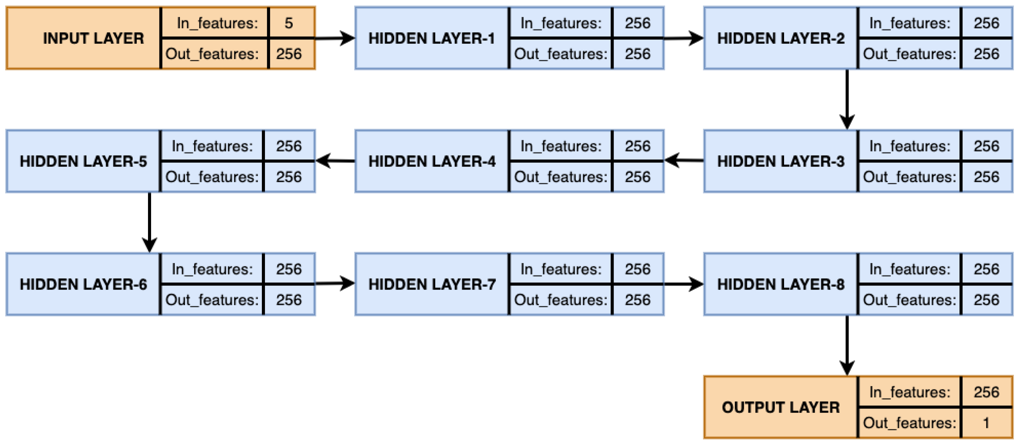
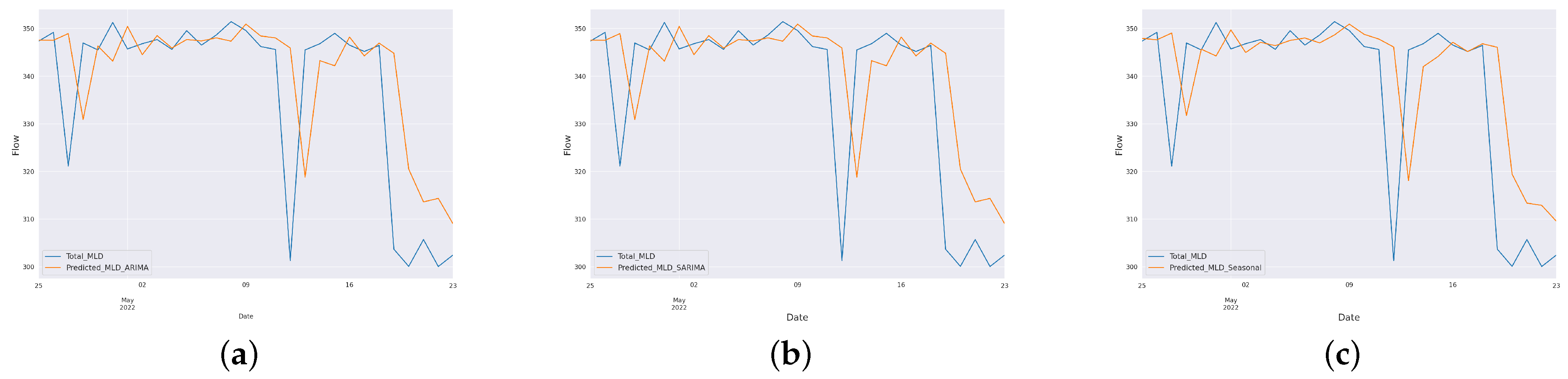
The paper aimed to predict the influent and effluent quality parameters of the WWTP using different machine learning models, namely ARIMA [11], SARIMA [12] and the proposed SARIMA with seasonal order. Among these models, the proposed SARIMA with seasonal order gave better predictions of influent parameters. For effluent parameter prediction, we used kNN [13], gradient boosting [14], random forest [15] and a proposed artificial neural network (ANN) [16] model. Among these, the proposed ANN outperformed the others. The proposed SARIMA with seasonal order and proposed artificial neural network models are the important components of the proposed model wPred which is elaborated in detail in Section 3.

The model wPred presented in this paper is specifically designed and implemented for the Bharwara WWTP. However, with a specific training component or perhaps after minor model improvements, the implemented model will be suitable for any wastewater treatment facility that is based on the UASB. This paper is organized as follows: Section 2 includes the related works in the field followed by methodology in Section 3, and the experimental findings are summarized with visualisation in Section 4. Section 5 discusses the conclusions and future works.

2. Related Works

This section outlines recent studies that have been conducted on the issue of wastewater treatment and parameter prediction. In [17], the authors explain the input parameters COD, BOD and TSS, based on an artificial neural network to propose a model for the prediction of TSS. For the Konya Wastewater treatment facility, model performance was shown using MSE and R value/correlation coefficient. With the use of neural networks with different hidden layers, the proposed model produced good results, with the training set’s correlation coefficient rising to 0.99.

In order to forecast the total nitrogen (T-N) concentration in the plant, ANN and SVM models were used in [18]. The $R^2$ value, relative efficiency and Nash–Sutcliff efficiency [19] criteria were applied to the model’s evaluation. Latin hypercube one factor at a time (LH-OAT) [20] and a pattern search method were used in a sensitivity analysis, which revealed that the ANN model outperformed the SVM model [16].

In [21], a study on rainwater discharge and a methodology for estimating BOD, TSS, COD and TDS in wastewater were also presented. Modeling was conducted using the support vector analysis and regression tree algorithms, and performance was measured using the $R^2$ value and the root-mean-squared error. The SVR model outperformed the regression tree for TSS, COD and TDS, while the regression tree outperformed SVR for BOD.

Online monitoring of wastewater quality was demonstrated in [22]. The concentrations of TSS, O&G and COD were monitored using a turbidimeter and UV/VIS spectroscopy. The signals from the two sensors were combined using a sensor fusion technique. The model was created using the boosting-partial least squares (boosting-PLS) method, which uses fused data to forecast wastewater quality.

In [23], the influent quality was predicted using four machine learning techniques: linear regression [24], ridge [25], ElasticNet [26], and lasso. Different techniques showed good accuracy for predicting influent parameters for various conditions. The outcomes reported in the reference made use of these models as warning modules to help with WWTP daily operations.

Ref. [27] explains the efficiency of the treatment plant for the removal of effluent particles, namely nitrogen was predicted by a model based on artificial intelligence. An SVM [28], ANFIS trapezoidal MF model [29], and an ANFIS Gbell MF model [29] were separate models created in Matlab. Parameters pH, $N{H}_3$, nitrogen, free ammonia and Kjeldahl $N_2$ were measured as influence parameters. By using the RMSE, NSE and correlation coefficient, performance was evaluated (R). An SVM networks model produced good outcomes.

The monitoring of intake and output parameters as well as the evaluation of STP’s efficacy were the main objectives in [30]. In order to identify similar sites, the cluster analysis technique was used to discover some connections between the present site and other sites. Measurements of the amounts of sulfate, nitrates, chloride, phosphate and bicarbonates revealed that STP efficiency was not up to par.

As the population increases rapidly, huge consumption of water is being recorded, leading to a drastic increase in the generation of wastewater; hence efficient wastewater treatment plants are needed. The authors in [17,18,22,23,27,30] have worked on the problem but their solutions are specific to their plants which are situated in different geographical locations. Therefore, a model is required for efficient utilization of a UASB-based wastewater treatment plant. The methodology for the proposed model is explained in the following section.

3. Methodology: wPred

To predict influent and effluent parameters, we propose our novel model named wPred that has three broad steps as given in Figure 2. A detailed description to each step is given in Section 3.1, Section 3.2 and Section 3.3.

Figure 2 explains the overall flow of the proposed model starting with data collection, followed by data preprocessing and then the influent and effluent quality parameters’ prediction.

3.1. Data Collection

From the Bharwara WWT Plant, we gathered a real-time data set comprising influent and effluent samples for the 38 months (April 2019 to May 2022) pre-, during and post-COVID-19. Selected influent and effluent samples were collected, captured, and recorded manually at the facility available at the plant. Table 1 shows the locations where the samples were gathered and their details. For influent samples, we recorded pH, DO, TSS, COD, BOD and Flow in MLD from all three inlet chambers for a total of 1138 days, while for effluent samples, we recorded pH, DO, TSS, COD and BOD for the same number of days.

3.2. Data Preprocessing

The dataset collected had a total of 1138 entries, which includes a certain number of missing values. Thereafter, we removed any row with a missing value. This leaves us with 1128 records with non-null values. The collected data set had MLD values for 3 different inlets, A, B and C, as shown in Figure 1. For data preprocessing, we added all 3 inlet loads to obtain total MLD as shown in

Table 3. Inlet description.

	Day	IN_PH	IN_DO	IN_TSS	IN_COD	IN_BOD	Total_MLD
mean	568	7	2	160	259	186	330
std	328	2	3	113	56	65	39
50%	566	7	0	214	251	160	347

. The statistical observations for the recorded influent and effluent samples are listed in Table 3 and

Table 4. Outlet description.

	Day	OUT_PH	OUT_DO	OUT_TSS	OUT_COD	OUT_BOD
mean	568	7	6	30	64	40
std	328	3	2	18	17	21
50%	566	7	5	40	68	27

, respectively.

Outlier analysis was conducted using a boxplot as shown in Figure 3 for total influent MLD corresponding to each day of the week. We can observe that nearly every week has the same amount of inflow, while days 0 and 1 have more outliers than the days 2–6, where 0 represents Sunday and 6 represents Saturday.

3.3. Model Designing

We desiged machine-learning-based models for the prediction of influent and effluent quality parameters separately. These models are elaborated in Section 3.3.1 and Section 3.3.2.

3.3.1. Model for Influent Parameter Prediction

The process flow for the proposed model for influent parameters is given in Figure 4. Firstly, on the acquired/preprocessed data, we analyzed the influent quality parameters in pre-COVID-19, during COVID-19 and post-COVID-19 durations. Further, we applied the model for time series forecasting of the influent parameter involving a series of steps as discussed here. We identified individual components of the time series such as trend and seasonality by decomposing the series. The auto correlation function (ACF) [31] and partial auto correlation function (PACF) [32] calculate the correlation between a current observed value and its lagged value. To check for stationarity of the data, we used the Dickey–Fuller Test [33] and rolling mean and standard deviation. Finally, the ARIMA [34] model and the SARIMA (to capture the seasonal behaviour) were applied to the total flow. Then, the predictions are made on the held out data from the last 29 days, i.e., from 25 April 2022 to 23 May 2022. The models are described briefly as follows.

ARIMA

A time series’ own prior values, especially its own lags and lagged prediction errors, are used in the auto regressive integrated moving average (ARIMA) [11] class of regression analysis models to “explain” the time series and predict future values. Any “non-seasonal” time series with patterns and more than random noise can be modelled using ARIMA models [34].

An ARIMA model is defined by the terms P, D and Q that are AR words arranged in P order of the MA term. Q and D stand for the amount of differencing required to make the time series stationary. The autoregressive (p) model of ARIMA (1,1,1) is as follows:

$$y_t=C+\varphi .y(t-1)+\dots +{\varphi }_p.y(t-p)+{ϵ}_t$$

(1)

where $y_t$ is the data, and $\varphi$ is the AR coefficient.

SARIMA

Seasonal ARIMA is applied when there is a seasonal fluctuation in a time series [12]. The seasonal moving average notation (Q) and the seasonal autoregressive notation (P) will be used to illustrate the multiplicative process of SARIMA [35]. The equation of SARIMA is as follow:

$$\begin{array}{c}\hfill y_t=C+\sum _{i=1}^P{\varphi }_i.y(t-1)+\sum _{i=1}^P.{\mathsf{\Phi }}_i.y(t-is)+{ϵ}_t..-\\ \hfill \sum _{i=1}^q{\varphi }_i.ϵ(t-i)+\sum _{i=1}^Q{\mathsf{\Theta }}_i.ϵ(t-is)\end{array}$$

(2)

where $y_t$ and $\varphi$ are as defined previously, $\theta$ is the MA coefficient, and $\mathsf{\Phi }$ and $\mathsf{\Theta }$ are the seasonal counterparts. Here, we applied SARIMA with seasonal order to predict influent parameters. The two evaluation metrics for the forecasting performance that we consider are mean absolute percentage error (MAPE) and symmetric mean absolute percentage error (sMAPE). Details of each are briefed below:

MAPE

It is given by the formula

$$MAPE=\frac{1}{n}\sum _{t=1}^n\left|\frac{A_t-F_t}{A_t}\right|$$

(3)

where A and F are actual and forecast values. It is often multiplied by 100 and expressed as a percentage which helps in comparing forecasts. Since it is asymmetric, it puts more penalty on negative errors (when forecast value is higher than actual value) than positive errors. Hence, MAPE favors the models that under-forecast rather than over-forecast.

sMAPE

It is a slightly modified form of MAPE and is given by the formula:

$$\begin{array}{c}\hfill sMAPE=\frac{1}{n}\sum _{t=1}^n\left|\frac{F_t-A_t}{\frac{A_t+F_t}{2}}\right|\end{array}$$

(4)

It overcomes the asymmetry problem of MAPE, where boundlessness of forecasts are higher than the actual.

3.3.2. Model for Effluent Parameter Predictions

A process flow of the overall proposed model for the effluent parameter prediction implemented in the paper is shown in Figure 5. The collected dataset is preprocessed followed by the design of the ML models. The next step is splitting the preprocessed data into the ratio of 70:30 labelled as training and testing datasets. The models are then trained on the training dataset, and then we tested the trained models on the unseen testing dataset.

In this paper, for predicting effluent parameters of the plant, different machine learning models, namely kNN [13], gradient boosting [14], random forest [15] and ANN [8] were used. The features description of these models are shown in

Table 5. ML algorithm details.

ML Algorithm	Feature Description
kNN	14 neighbours
	leaf size: 30
	Algorithm to compute neighbours: KDTree
Gradient Boosting Regression	Max Depth: 3
	100 estimators
	Loss Function: Squared Error
Random Forest Regression	100 estimators
	base estimator: Decision Tree Regressor
	Split criterion: Squared Error
Artificial Neural Network	1000 epochs
	Xavier Initialization Weights
	ReLU activation function
	sigmoid activation function

. The k-nearest neighbour [13] regression technique uses the shortest distance between nearest neighbours to forecast the effluent, using influents as the predicting factors. Here, the ideal nearest neighbour was found to be 14 as listed in Table 5. The gradient boosting regression [14] technique uses an ensemble of multiple separate decision trees, with the output from one layer serving as the input to the next to forecast the effluent using influents as the predicting variables. A depth of 3 and 100 estimators was used as listed in Table 5. The random forest regression [15] method employs an ensemble of multiple separate decision trees to predict effluent concurrently, while using influents as the predicting variables. The implementation of the model includes 100 estimators, and decision tree regressor is used as base estimator as listed in Table 5.

WWTP processes are modelled using artificial neural network (ANN) models due to their great adequacy, efficiency, and fairly promising applications in engineering. They can be used to improve process performance prediction [5,8,9]. Typically, an ANN makes use of process-relevant historical data. An information processing system, ANN is inspired by organic nerve systems. A neural network’s goal is to generate output values from input values using complex internal computations [16]. Pattern recognition, identification, classification, speech, vision, and automation are just a few of the complicated tasks that neural networks are trained to carry out [36]. Figure 6 describes the layers and the parameters used in the construction of the ANN-based prediction model for the effluent quality parameters.

The following is a list of model properties:

• Inputs to the model: BOD, pH, COD, TSS and MLD at the inlet.
• Model outputs include: Each parameter’s BOD, pH, COD, TSS, DO and MPN, one-by-one considering all input parameters listed above.
• Dataset split into 70:30 ratio for training and testing.
• Mean square error is an estimator function.

Mean square error (MSE) is used to gauge how well the model is performing. The following is the MSE formula:

$$MSE=\frac{1}{n}.\sum _{i=1}^n.{(y_i-y_i^{\wedge })}^2$$

(5)

The results and the evaluation of the proposed model wPred (for both influent and effluent parameters) are shown in Section 4.

4. Results and Evaluation

The result and evaluation of wPred as designed and implemented for prediction of both influent and effluent parameters are explained in Section 4.2 and Section 4.3 after the implementation details.

4.1. Implementation Details

The model wPred is developed in Python using ML libraries. Details of the implementation environment are given in

Table 6. Implementation environment.

Language	Python (version 3.11.0)
Tool	Google Colaboratory
Libraries	Pandas, NumPy, Scikit Learn, Matplotlib, Seaborn and SciPy

.

4.2. Results of Influent Parameter Prediction

We observed continuous fluctuating downfall in MLD from the end of March 2020 (during the peak of the first wave of COVID-19) to July 2021 as shown in Figure 7a, with a mean value of 337.34, standard deviation of 25.74 and variance of 662.46, respectively. Similarly, from January 2021 to March 2022 MLD values show little fluctuation except towards the end of September to mid-October 2021 and in March 2022. Moreover, BOD and COD influent parameters attained their minimum values during the peak of the first wave in Uttar Pradesh compared to the other durations as shown in Figure 7b,c, respectively.

Time-series data can be considered as a combination of four components, namely level (the average value), trend, seasonality (repeating cycles) and residual noise. The decomposition of flow in these four components is depicted in Figure 8. We observe that the trend in data changes from low to high in the middle months, and then it stays at a constant pace thereafter as can be seen from Figure 8.

Figure 9 shows the rolling mean and standard deviation of the data. We can clearly see the rolling standard deviation is not aligned with the original data, so we apply integration. After applying the integration, we can observe from Figure 9 that the rolling standard is in alignment with the integrated dataset. We need not to further apply the integration, and we achieve stationarity with d order of one. The p-value of 0.000085 is very good if we use the 5% critical value; this series has no continuous growing graph. After differencing, the p-value is extremely small. Thus, this series is very likely to be stationary.

Based on the ACF [31] and PACF [32] plots as shown in Figure 10 and Figure 11, we see a sudden cut to the PACF at Lag 3, and ACF gradually decreases from Lag 3. Thus, we infer the AR (p) value with three will give the better result, and for selecting the order of MA (q), we select just the opposite value, i.e., we select the MA (q) to be three.

A normality test for the residuals is conducted, respectively, for three models, and the test statistic and p-value are calculated. Based on these, plots are generated as shown in Figure 12, and the mean and standard deviation are recorded.

The forecasting results for the last 29 days of the dataset were obtained for the three models as shown in Figure 13. We can see that the wSARIMA model with seasonal order effectively predicts the actual flow with MAPE of 2.66 and sMAPE of 2.59 as shown in

Table 7. Evaluation metrics.

Metrics	Model
ARIMA	SARIMA	Seasonal Ordered SARIMA
MAPE	2.72	2.72	2.67
sMAPE	2.64	2.64	2.59

. Meanwhile, vanilla ARIMA and SARIMA models also perform well, and we obtain MAPE and sMAPE as 2.72 and 2.64, which is in the acceptable range of 0–5% and highly acceptable for time-series forecasts. The results of the effluent parameters using the proposed effluent prediction model is explained in Section 4.3.

4.3. Results of Effluent Parameter Prediction

The values of the effluent parameters are predicted based on the influent parameters, namely dissolved oxygen (DO), pH value (pH), chemical oxygen demand (COD), total suspended solids (TSSs), biochemical oxygen demand (BOD) and myeloproliferative neoplasms (MPN). For predicting effluent parameters of the plant, we implemented four machine learning models, namely kNN [13], gradient boosting [14], random forest [15] and the proposed ANN model as per the features as described in in the Table 5. Architecture for the proposed ANN model is given in Figure 6. We obtained the prediction accuracy for each effluent parameter, namely pH, BOD, COD, DO, TSS and MPN using all four machine learning models namely, kNN, Gradient Boosting, Random Forest and the proposed ANN model. These prediction test accuracy are recorded in the form of comparison chart as shown in

Table 8. Comparison table for the predicted testing accuracy for effluent parameters.

	KNN	Gradient Boosting	Random Forest	ANN
OUT_PH	70.45	71.23	71	74.55
OUT_BOD	8.40	9.29	12.83	56.12
OUT_COD	4.86	3.09	9.29	60.88
OUT_DO	15.48	14.60	11.50	51.11
OUT_TSS	6.63	8.40	9.39	65.41
OUT_MPN	4.42	3.53	4.86	52.65

.

Table 9. R and MSE values of ANN model on the testing dataset for the effluent parameters.

	OUT_PH	OUT_BOD	OUT_COD	OUT_DO	OUT_TSS	OUT_MPN
R	0.89	0.74	0.827	0.99	0.92	0.89
MSE	0.06	0.014	0.02	0.023	0.038	0.069

depicts proposed ANN model’s performance using the mean squared error and the correlation coefficient (R value). The minimum cost achieved in proposed ANNs is around 3e-3+5. The proposed model performed efficiently, when neural networks with different hidden layers were used. The correlation coefficient in the testing set rose as high as 0.99. After comparing the efficiency of the abovementioned models, we concluded that our proposed ANN model, which predicts more than 50% for each of the effluent correctly, is best for our use case.

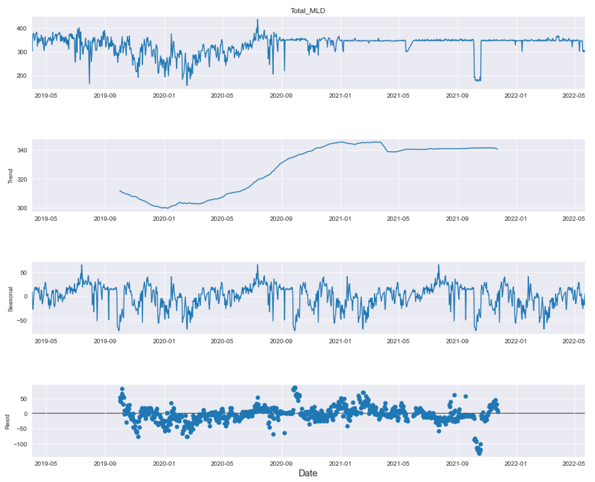
5. Conclusions and Future Works

In this paper, we have designed and implemented a novel model wPred to predict/forecast wastewater (influent) parameters, namely incoming load (total MLD), and effluent parameters, namely MPN, BOD, COD, DO, TSS and pH for the real-time data obtained pre-, during and post-COVID-19 period from a UASB-based Bharwara WWTP in Asia. The categorization of influent and effluent model design wPred further divides the problem into two sub-problems, where the influent total MLD value is forecasted using ARIMA and seasonal ARIMA models, whereas the effluent parameters are predicted and compared using four machine learning models: kNN, random forest, gradient boosting regression and the proposed artificial neural network model. Forecasting the incoming load gives promising results with an extremely low symmetric mean absolute prediction error of 2.59% indicating high prediction accuracy in the proposed model wPred. Moreover, the estimation of effluent parameters with the help of the proposed ANN model results in a significant rise in accuracy compared to the existing machine learning models, as high as 74.55% (for effluent pH), a significantly low mean squared error (0.014 for effluent BOD), and a strong correlation (R-value) up to 0.99 (for effluent DO) in the proposed model wPred. The results of the proposed model wPred provide a way forward in reducing the manual effort of recording the wastewater quality parameters and also helps in forecasting the incoming load based on seasonal variations effectively. Future works include the addition of a larger dataset which would more clearly explain how different parameters affect one another. We also plan to design a more generalized model applicable for a large class of UASB-based WWTPs.

References

1. Majumder, S.; Poornesh, M.B.; Reethupoonar, R.M. A review on working, treatment, and performance evaluation of sewage treatment plant. Int. Eng. Res. Appl. 2019, 9, 1–49. [Google Scholar]
2. Krewski, D.; Yokel, R.A.; Nieboer, E.; Borchelt, D.; Cohen, J.; Harry, J.; Kacew, S.; Lindsay, J.; Mahfouz, A.M.; Rondeau, V. Human health risk assessment for aluminium, aluminium oxide, and aluminium hydroxide. J. Toxicol. Environ. Health Part B 2007, 10, 1–269. [Google Scholar]
3. Asiwal, R.S.; Sar, S.K.; Singh, S.; Sahu, M. Wastewater treatment by effluent treatment plants. SSRG Int. J. Civil Eng. 2016, 3, 12. [Google Scholar]
4. Newhart, K.B.; Holloway, R.W.; Hering, A.S.; Cath, T.Y. Data-driven performance analyses of wastewater treatment plants: A review. Water Res. 2019, 157, 498–513. [Google Scholar] [CrossRef] [PubMed]
5. Maier, H.R.; Dandy, G.C. Neural networks for the prediction and forecasting of water resources variables: A review of modelling issues and applications. Environ. Model. Softw. 2000, 15, 101–124. [Google Scholar] [CrossRef]
6. Gernaey, K.V.; Van Loosdrecht, M.C.; Henze, M.; Lind, M.; Jørgensen, S.B. Activated sludge wastewater treatment plant modelling and simulation: State of the art. Environ. Model. Softw. 2004, 19, 763–783. [Google Scholar] [CrossRef]
7. Vesilind, P. Wastewater Treatment Plant Design; IWA Publishing: London, UK, 2003; Volume 2. [Google Scholar]
8. ASCE Task Committee on Application of Artificial Neural Networks in Hydrology. Artificial neural networks in hydrology. II: Hydrologic applications. J. Hydrol. Eng. 2000, 5, 124–137. [Google Scholar] [CrossRef]
9. Neelakantan, T.R.; Brion, G.M.; Lingireddy, S. Neural network modelling of Cryptosporidium and Giardia concentrations in the Delaware River, USA. Water Sci. Technol. 2001, 43, 125–132. [Google Scholar] [CrossRef] [PubMed]
10. Yadav, P.; Chaudhary, A.; Keshari, A.; Chaudhary, N.K.; Sharma, P.; Kumar, S.; Yadav, B.S. Data Visualization of Influent and Effluent Parameters of UASB-based Wastewater Treatment Plant in Uttar Pradesh. Int. J. Adv. Comput. Sci. Appl. 2022, 13, 1–10. [Google Scholar] [CrossRef]
11. Gilbert, K. An ARIMA supply chain model. Manag. Sci. 2005, 51, 305–310. [Google Scholar] [CrossRef]
12. Nobre, F.F.; Monteiro, A.B.S.; Telles, P.R.; Williamson, G.D. Dynamic linear model and SARIMA: A comparison of their forecasting performance in epidemiology. Stat. Med. 2001, 20, 3051–3069. [Google Scholar] [CrossRef] [PubMed]
13. Guo, G.; Wang, H.; Bell, D.; Bi, Y.; Greer, K. November. KNN model-based approach in classification. In OTM Confederated International Conferences “On the Move to Meaningful Internet Systems”; Springer: Berlin/Heidelberg, Germany, 2003; pp. 986–996. [Google Scholar]
14. Natekin, A.; Knoll, A. Gradient boosting machines, a tutorial. Front. Neurorobot. 2013, 7, 21. [Google Scholar] [CrossRef] [PubMed]
15. Biau, G.; Scornet, E. A random forest guided tour. Test 2016, 25, 197–227. [Google Scholar] [CrossRef]
16. Matala, A. Sample Size Requirement for Monte Carlo Simulations Using Latin Hypercube Sampling. Ph.D. Thesis, Helsinki University of Technology, Department of Engineering Physics and Mathematics, Systems Analysis Laboratory, Helsinki, Finland, 2008; p. 25. [Google Scholar]
17. Tumer, A.E.; Edebali, S. An artificial neural network model for wastewater treatment plant of Konya. Int. J. Intell. Syst. Appl. Eng. 2015, 3, 131–135. [Google Scholar] [CrossRef]
18. Guo, H.; Jeong, K.; Lim, J.; Jo, J.; Kim, Y.M.; Park, J.P.; Kim, J.H.; Cho, K.H. Prediction of effluent concentration in a wastewater treatment plant using machine learning models. J. Environ. Sci. 2015, 32, 90–101. [Google Scholar] [CrossRef]
19. McCuen, R.H.; Knight, Z.; Cutter, A.G. Evaluation of the Nash–Sutcliffe efficiency index. J. Hydrol. Eng. 2006, 11, 597–602. [Google Scholar] [CrossRef]
20. Chen, R.B.; Hsieh, D.N.; Hung, Y.; Wang, W. Optimizing Latin hypercube designs by particle swarm. Stat. Comput. 2013, 23, 663–676. [Google Scholar] [CrossRef]
21. Qin, X.; Gao, F.; Chen, G. Wastewater quality monitoring system using sensor fusion and machine learning techniques. Water Res. 2012, 46, 1133–1144. [Google Scholar] [CrossRef]
22. Wang, R.; Pan, Z.; Chen, Y.; Tan, Z.; Zhang, J. Influent Quality and Quantity Prediction in Wastewater Treatment Plant: Model Construction and Evaluation. Pol. J. Environ. Stud. 2021, 30, 4267–4276. [Google Scholar] [CrossRef]
23. Manu, D.S.; Thalla, A.K. Artificial intelligence models for predicting the performance of biological wastewater treatment plant in the removal of Kjeldahl Nitrogen from wastewater. Appl. Water Sci. 2017, 7, 3783–3791. [Google Scholar] [CrossRef]
24. Weisberg, S. Applied Linear Regression; John Wiley & Sons: Hoboken, NJ, USA, 2005; Volume 528. [Google Scholar]
25. McDonald, G.C. Ridge regression. Wiley Interdiscip. Rev. Comput. Stat. 2009, 1, 93–100. [Google Scholar] [CrossRef]
26. Zou, H.; Hastie, T. Regularization and variable selection via the elastic net. J. R. Stat. Soc. Ser. A 2005, 67, 301–320. [Google Scholar] [CrossRef]
27. Gautam, S.K.; Sharma, D.; Tripathi, J.K.; Ahirwar, S.; Singh, S.K. A study of the effectiveness of sewage treatment plants in Delhi region. Appl. Water Sci. 2013, 3, 57–65. [Google Scholar] [CrossRef]
28. Schuldt, C.; Laptev, I.; Caputo, B. Recognizing human actions: A local SVM approach. In Proceedings of the 17th International Conference on Pattern Recognition, ICPR, Washington, DC, USA, 23–26 August 2004; IEEE: New York, NY, USA, 2004; Volume 3, pp. 32–36. [Google Scholar]
29. Fragiadakis, N.G.; Tsoukalas, V.D.; Papazoglou, V.J. An adaptive neuro-fuzzy inference system (anfis) model for assessing occupational risk in the shipbuilding industry. Saf. Sci. 2014, 63, 226–235. [Google Scholar] [CrossRef]
30. Alnaa, S.E.; Ahiakpor, F. ARIMA (autoregressive integrated moving average) approach to predicting inflation in Ghana. J. Econ. Int. Financ. 2011, 3, 328–336. [Google Scholar]
31. Wise, J. The autocorrelation function and the spectral density function. Biometrika 1955, 42, 151–159. [Google Scholar] [CrossRef]
32. Ramsey, F.L. Characterization of the partial autocorrelation function. In The Annals of Statistics; Institute of Mathematical Statistics: Beachwood, OH, USA, 1974; pp. 1296–1301. [Google Scholar]
33. Cheung, Y.W.; Lai, K.S. Lag order and critical values of the augmented Dickey–Fuller test. J. Bus. Econ. Stat. 1995, 13, 277–280. [Google Scholar]
34. Piccolo, D. A distance measure for classifying ARIMA models. J. Time Ser. Anal. 1990, 11, 153–164. [Google Scholar] [CrossRef]
35. Valipour, M. Long-term runoff study using SARIMA and ARIMA models in the United States. Meteorol. Appl. 2015, 22, 592–598. [Google Scholar] [CrossRef]
36. Yegnanarayana, B. Artificial Neural Networks; PHI Learning Pvt. Ltd.: New Delhi, India, 2004. [Google Scholar]
Figure 1. The Bharwara Wastewater Treatment Plant.
Water 15 00710 g001
Figure 2. Process flow for the proposed wPred model.
Water 15 00710 g002
Figure 3. Total MLD flow based on weekdays.
Water 15 00710 g003
Figure 4. Process flow for the proposed influent parameter prediction.
Water 15 00710 g004
Figure 5. Process flow for the effluent parameter prediction.
Water 15 00710 g005
Figure 6. Architecture: ANN based influent prediction model.
Water 15 00710 g006
Figure 7. Total (a) MLD; (b) COD; (c) BOD.
Water 15 00710 g007
Figure 8. Seasonal Decompose.
Water 15 00710 g008
Figure 9. Rolling mean and standard deviation: (a) total flow; (b) first difference; (c) seasonal first difference.
Water 15 00710 g009
Figure 10. ACF (a) PACF (b) of total flow and first difference.
Water 15 00710 g010
Figure 11. ACF and PACF: (a) ARIMA; (b) SARIMA; (c) SARIMA with seasonal order.
Water 15 00710 g011
Figure 12. Residual for ARIMA (a), SARIMA (b) and SARIMA (c) with seasonal order.
Water 15 00710 g012
Figure 13. Prediction results: (a) ARIMA; (b) SARIMA; (c) SARIMA with seasonal order.
Water 15 00710 g013