Coupled Model for Assessing the Present and Future Watershed Vulnerabilities to Climate Change Impacts

Abstract

There is great uncertainty about the future effects of climate change on the global economic, social, environmental, and water sectors. This paper focuses on watershed vulnerabilities to climate change by coupling a distributed hydrological model with artificial neural networks and spatially distributed indicators for the use of a predictive model of such vulnerability. The analyses are complemented by a Monte Carlo evaluation of the uncertainty associated with the projections of the global circulation models, including how such uncertainty impacts the vulnerability forecast. To test the proposal, the paper uses current and future vulnerabilities of the Turbio River watershed, located in the semi-arid zone of Guanajuato (Mexico). The results show that nearly 50% of the watershed currently has medium and high vulnerabilities, and only the natural areas in the watershed show low vulnerabilities. In the future, an increase from medium to high vulnerability is expected to occur in urban and agricultural areas of the basin, with an associated uncertainty of ±15 mm in the projected precipitation.

1. Introduction

Watershed vulnerabilities to climate change in the economic, social, environmental, and water sectors, and their associated uncertainties in calculations, are great hydrological challenges in the 21st century [1]. Millions of people (and sectors) around the world, including the economic, social, environmental, and water sectors, are affected each year by climate disasters [2]. In recent decades, the impacts of climate change have already become visible, mainly in the increase in temperatures [3], and the increase and/or decrease in precipitation in various regions across the world [4,5]. Consequently, the already-stressed hydrological systems and resources are under greater pressure [6]. For instance, many world regions face issues due to water scarcity and flooding events [7]. Despite multiple scientific efforts [2], assessing the vulnerability to climate change is not an easy task due to the large number of variables involved and the associated growing uncertainty, especially in the future.

The most common methodology to quantify vulnerability to climate change is based on a set of indicators combined into a single index [8]. For example, multiple linear regression has been used to determine aquifer vulnerability to nitrate pollution in groundwater [9], principal component analysis to create spatially explicit aggregate indices of vulnerability [10], and analytical hierarchy processes mixed with fuzzy comprehensive evaluation methods have been applied to achieve the drought vulnerability assessment [11]. In particular, such composite indices are used in environmental and risk models integrated with geographic information. Among them, the following instances stand out: the sustainability synthetic territorial index, which is a composite indicator that includes the environmental, economic, and institutional nature [12]; the vulnerability of the area surrounding an industrial site using a multi-criteria decision approach [13]; the climate change vulnerability to predict the variation in risk perception [14]; and the prediction of groundwater vulnerability in a spatial context [15].

Vulnerability to climate change estimated by the existing state-of-the-art models does not consider all the variables involved in the system, limiting its accuracy. In an attempt to use climatic variables in the vulnerability assessment, general circulation models (GCMs) are the most used methods to project future climate [16,17,18]. GCMs simulate the climate variables by solving complex differential equations capable of basing their projections on representative concentration pathway (RCP) scenarios [19] that represent greenhouse gas emissions. GCMs are major sources used to explore the complexity of climate and give quantitative measures of future weather [18]. However, their uses are limited at the watershed scale because GCM projections are global in scale. Still, future projections of climate change are some of the main challenges regarding the correct quantifications (as they occur to watershed vulnerabilities). To this end, downscaling is a method that adapts climatic variables to local, fine-scaled conditions, such as those at a river basin scale [20].

GCM downscaling via flexible methods, such as artificial neural networks (ANNs), have become popular in recent years [20]. The downscaling technique has been applied to adapt the GCM projections to a basin scale [18,19,21]. Authors such as [22,23,24] recommend investigating the uncertainties associated with the projections of meteorological variables with ANN. Uncertainty in hydrological predictions can originate from several main sources, and it has been reported that the primary sources of uncertainty come from model input data [25,26,27]. Data uncertainty propagates to hydrological analyses that may lead to wrong interpretations. Hence, the generation of quantitative measures of confidence in a model’s results is essential to guiding the weight that should be given to the model in decision-making [28,29]. The Monte Carlo simulation is a statistical method used for the simulation of stochastic processes that can be used to calculate uncertainty. In hydrological analyses, the method draws samples of possible data values from defined uncertainty models. Each sample is used to compute the derived value of interest [28].

This paper proposes calculating the current watershed vulnerability to climate change by coupling a distributed hydrological model, artificial neural network, and spatially distributed indicator, as well as their evolution in the near future, according to the GCM projections and Intergovernmental Panel on Climate Change (IPCC) scenarios. The paper includes a combination of artificial neural networks and the Monte Carlo method to quantify the uncertainty associated with downscaling global circulation models and determine how this uncertainty affects the vulnerability forecast.

2. Methodology

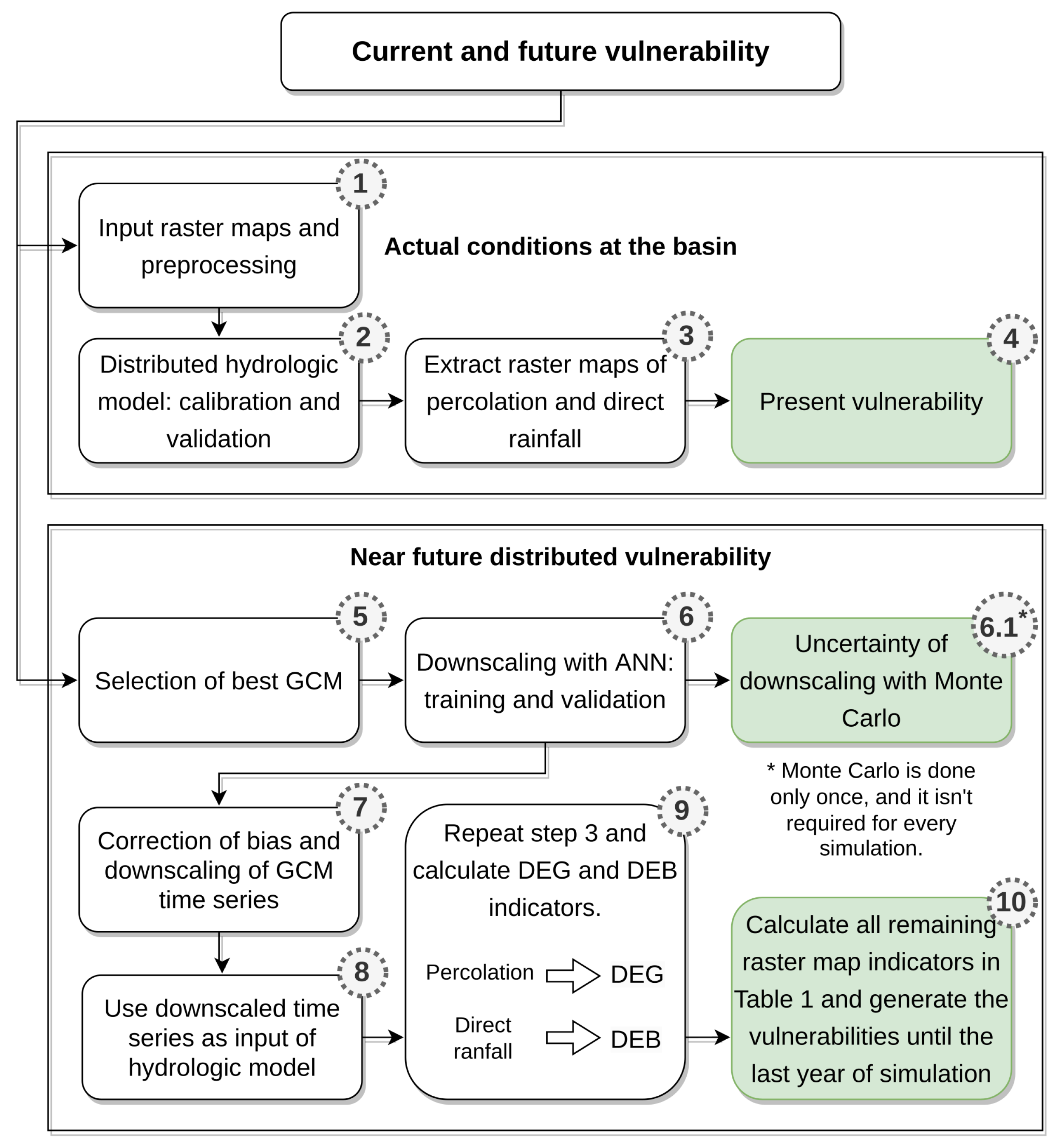
This paper proposes the creation of a distributed vulnerability to climate change by coupling a distributed hydrological model and an ANN model with spatially distributed indicators. Reference [30] can be considered an antecedent of this work. However, the current proposal incorporates a significant step forward as the downscaling is approached by the use of ANN models. In addition, the current paper works with historical weather station records and GCM projections directly and annually calculates distributed vulnerabilities for all simulation models. The downscaling process only considers the spatial resolution of the GCM precipitation projections for the Inter-Comparison of Coupled Models-Phase-5 Project (CMIP5), which include the RCP4.5, RCP6.0, and RCP8.5 emission scenarios [31]. In addition, we used the Monte Carlo simulation to model the uncertainty associated with such projections and an analysis of its impact on the vulnerability quantification. Ultimately, the work was developed within a framework that encompassed a predictive vulnerability model (MPDV2.0) and ANN downscaling, as well as integrated GCM projections in CMIP5 [32] and IPCC scenarios [33]. The foregoing followed the scheme shown in Figure 1, where the hydrological simulation for current conditions was conducted first and, as a result, the current vulnerability of the basin was assessed by taking the raster maps of percolation and direct rainfall. A second phase of this work addresses future watershed vulnerabilities to climate change. To this end, a GCM downscaling with ANN will correct the model bias in the training and validation processes by decreasing the error; moreover, the number of points with information was increased in the downscaling by taking the GCM nearest points to each station, but not all of the points. The input/output of the ANN was the downscaled time series for the selected station. If the process was repeated at each station and there were more stations than GCM points, then the number of output time series was the same as the available stations. This downscaled time series was used as the input of the hydrological model so future percolation and rainfall maps were generated during the simulation. Finally, the near future distributed vulnerability was calculated using the hydrological analysis of the projected weather input.

2.1. Distributed Vulnerability Assessment

A predictive vulnerability model, such as MPDV2.0, calculates the distributed vulnerability of the watershed (MPDV2.0 is described in [30]) in contrast to the other methodologies [34,35,36,37]. The effects of climate and land-use changes are included in the vulnerability expression. MPDV2.0 calculates vulnerability based on the IPCC vision [38], which generally explains it using the degree of exposure to a threat, $GE$, and the sensitivity to such a threat, S. The approach considers the basin features that make the system more vulnerable to climate change from the point of view of each sector, and the capacity of the adaptation of the system, $CA$. In this regard, $CA$ represents the features of the basin and the actions that mitigate the effects of climate change. Equation (1) combines all of these components to represent the watershed vulnerabilities to climate change impacts,

$$V=f(GE,S,CA).$$

(1)

The variables of Equation (1) were obtained experimentally upon the 25 drought indicators proposed by [39] and, consequently, adapted to estimate the vulnerability following the steps in [30]. The indicators include socioeconomic, environmental, and water contributions to climate change vulnerability estimation. Every indicator consists of a division of maps with unique features of the basin; the arithmetic division is made with each corresponding raster cell. Once the raster maps are divided and the indicators obtained, they are standardized for comparison purposes in case they are computed in multiple watersheds. If the indicator is of type $CA$, it includes all indicators that minimize the vulnerability to climate change; and the first case of Equation (2) shall be used; for the rest of the indicators that maximize vulnerability, the second case shall be used. The Equation implemented to perform standardization on a given dataset, $X=\{x_1,\dots x_n\}$, follows the expression of Equation (2),

$$x_i^{*}\left(x_i\right)=\left\{\begin{array}{c}\frac{x_{\max }-x_i}{x_{\max }-x_{\min }},\mathrm{If}\mathrm{indicator}\in \mathrm{CA},\mathrm{minimize}\mathrm{vulnerability}\hfill \\ \frac{x_i-x_{\min }}{x_{\max }-x_{\min }},\mathrm{otherwise},\mathrm{maximize}\mathrm{vulnerability}\hfill \end{array}\right.$$

(2)

where $x_i^{*}$ is the normalized value of the variable values, $x_i$ is the i-th value of dataset X, $x_{min}$ and $x_{max}$ are the minimum and maximum values of the dataset. For each normalized indicator, a weight will be obtained using Equation (3),

$$w_i=\frac{\sqrt{{\sigma }_i^2}}{{\sum }_{i=1}^m\sqrt{{\sigma }_i^2}},$$

(3)

where $w_i$ is the weight of the i-th normalized indicator; $\sqrt{{\sigma }_i^2}$ is the standard deviation of the set of the i-th indicator values, and n is the number of indicators selected. The MPDV2.0 calculates the weighted mean from the normalized indicators that belong to the same sector, the results are economic (EV), social (SV), environmental (AV), and water (HV) vulnerabilities using the expression of Equation (4),

$$V=\sum _{i=1}^n{x}_i^{*}{w}_{V_j}\mathrm{For}V=\{EV,SV,AV,HV\},$$

(4)

where $w_{V_j}$ is the weight of the j indicator in the V sector.

Percolation and direct runoff were considered for computing the indicators for the cases of AV and HV. Changes in water availability through hydrological simulation were represented in every raster cell of the basin. Finally, MPDV2.0 calculated the global vulnerability, averaging the vulnerabilities of Equation (4).

2.2. Spatially Distributed Indicators

We calculated each indicator using the formulations presented in [30]; the indicator values were spatially distributed in raster cells of $90\times 90$ m. The geographic information used in estimating the indicators was obtained from the National Institute of Statistics and Geography (INEGI) available at https://www.inegi.org.mx/ accessed on 8 February 2023 and from the National Water Information System of the National Water Commission (SINA-CONAGUA) available at http://sina.conagua.gob.mx/sina/ accessed on 8 February 2023. They are government departments that allow free downloading of information at scales of 1:50,000 and 1:250,000. As the available information covers the country, the maps are clipped with the watershed of the case study.

Table 1. Equations and sources of information used in the calculation of indicators [30].

Name, Equation, and Units
Indicators	Economic	Population density: $PD=\frac{\mathrm{Number}\mathrm{of}\mathrm{inhabitants}}{\mathrm{Area}\left({\mathrm{km}}^2\right)}$; (habkm−2)
		Economically active population: $EAP=\frac{\mathrm{EAP}\mathrm{unemployed}}{\mathrm{Total}\mathrm{EAP}}$; (%)
		Length of rural roads: $LRR=\mathrm{Length}$; (km)
		Agricultural area for irrigation: $AAI=\mathrm{Amount}$; (ha)
		Agriculture area with technified irrigation: $ATI=\mathrm{Amount}$; (ha)
	Social	Population without medical services: $PWMS=\frac{\mathrm{Population}\mathrm{with}\mathrm{medical}\mathrm{services}}{\mathrm{Total}\mathrm{population}}$; (%)
		Population in poverty: $PP=\frac{\mathrm{Population}\mathrm{in}\mathrm{poverty}}{\mathrm{Total}\mathrm{population}}$; (%)
		Illiterate population: $IP=\frac{\mathrm{Illiterate}\mathrm{population}\mathrm{of}\mathrm{the}\mathrm{same}\mathrm{age}}{\mathrm{Inhabitants}\mathrm{of}\mathrm{the}\mathrm{same}\mathrm{age}}$; (%)
		Houses without drinking water: $HDW=\frac{\mathrm{Houses}\mathrm{number}\mathrm{without}\mathrm{drinking}\mathrm{water}}{\mathrm{Total}\mathrm{number}\mathrm{of}\mathrm{houses}}$; (%)
		Houses without drainage and no restroom: $HDR=\frac{\mathrm{Houses}\mathrm{number}\mathrm{without}\mathrm{drainage}\mathrm{and}\mathrm{no}\mathrm{restroom}}{\mathrm{Total}\mathrm{number}\mathrm{of}\mathrm{houses}}$; (%)
		Houses without electricity: $HWE=\frac{\mathrm{Houses}\mathrm{number}\mathrm{without}\mathrm{electricity}}{\mathrm{Total}\mathrm{number}\mathrm{of}\mathrm{houses}}$; (%)
		Houses with land floor: $HLF=\frac{\mathrm{Houses}\mathrm{number}\mathrm{with}\mathrm{land}\mathrm{floor}}{\mathrm{Total}\mathrm{number}\mathrm{of}\mathrm{houses}}$; (%)
	Environmental	Degree of exploitation of the basin: $DEB=\frac{\mathrm{Annual}\mathrm{volume}\mathrm{of}\mathrm{surface}\mathrm{extractions}}{\mathrm{Average}\mathrm{annual}\mathrm{runoff}\mathrm{volume}}$; $\left(dimensionless\right)$
		Degree of exploitation of groundwater: $DEG=\frac{\mathrm{Annual}\mathrm{volume}\mathrm{of}\mathrm{groundwater}\mathrm{extractions}}{\mathrm{Average}\mathrm{annual}\mathrm{recharge}\mathrm{of}\mathrm{the}\mathrm{aquifer}}$; $\left(dimensionless\right)$
		Deforestation: $DEF=\frac{\mathrm{Deforested}\mathrm{area}\left({\mathrm{km}}^2\right)}{\mathrm{Total}\mathrm{area}\left({\mathrm{km}}^2\right)}$; (%)
		Protected natural areas: $ANP=\frac{\mathrm{Protected}\mathrm{vegetation}\mathrm{cover}\mathrm{area}\left({\mathrm{km}}^2\right)}{\mathrm{Total}\mathrm{area}\left({\mathrm{km}}^2\right)}$; (%)
	Water	Degree of exploitation of the basin: $DEB=\frac{\mathrm{Annual}\mathrm{volume}\mathrm{of}\mathrm{surface}\mathrm{extractions}}{\mathrm{Average}\mathrm{annual}\mathrm{runoff}\mathrm{volume}}$; $\left(dimensionless\right)$
		Degree of exploitation of groundwater: $DEG=\frac{\mathrm{Annual}\mathrm{volume}\mathrm{of}\mathrm{groundwater}\mathrm{extractions}}{\mathrm{Average}\mathrm{annual}\mathrm{recharge}\mathrm{of}\mathrm{the}\mathrm{aquifer}}$; $\left(dimensionless\right)$

shows the economic, social, environmental, and water indicators for calculating vulnerability.

2.3. Downscaling GCM Time Series

One of the problems associated with GCMs is their large-scale resolution [40]. Hence, a downscaling process is required to lower such a resolution, fitting the variables simulated in the atmosphere with the variables measured in the basin, where a precipitation regimen can be identified. Among the multiple ways to approach downscaling, these highlighted methods are based on machine learning. This is the case with the excellent results provided by the ANN [41,42,43].

This paper proposes the use of an ANN multi-layer perceptron (MLP). MLP is the artificial neural network most used for practical applications and it consists of layers of adaptive weights with full connectivity between layers. The ANN-MLP structure is composed of the input and hidden and output layers of interconnected neurons. Among the multiple activation functions for neuron-level operations, the most common for the hidden layer is a hyperbolic tangent function, i.e., a sigmoid function suitable for the output layer. An ANN-MLP training phase starts by initializing the weights of the neuron’s interconnections to small random values. Those weights interact with each other moving forward through the neuron connections, from the input to the output layers. Then, a backpropagation process recomputes the weight values from the output to the input. The backpropagation involves the evaluation of the derivatives of an error function, computed at the output layer, with respect to the neural connection weights and biases. This process reduces the error at each iteration [44].

The process continues through the application of a downscaling process to the future projections of the GCMs of the CMIP5 project using ANN models. The output of this method is expected to correct the bias and reduce the error of climatic variables in the GCM. The ANN model is a traditional multilayer perceptron (MLP), which has a structure of I-H-O; where the inputs are a climatic variable from I points in the GCM model, H is the size of the hidden layer and the output of the network is the observed climatic variable in O stations. The GCM time series are extracted from the available points that cover the surface of the basin and then the ANN is trained with the observed times series, taking only the GCM data near the group of stations.

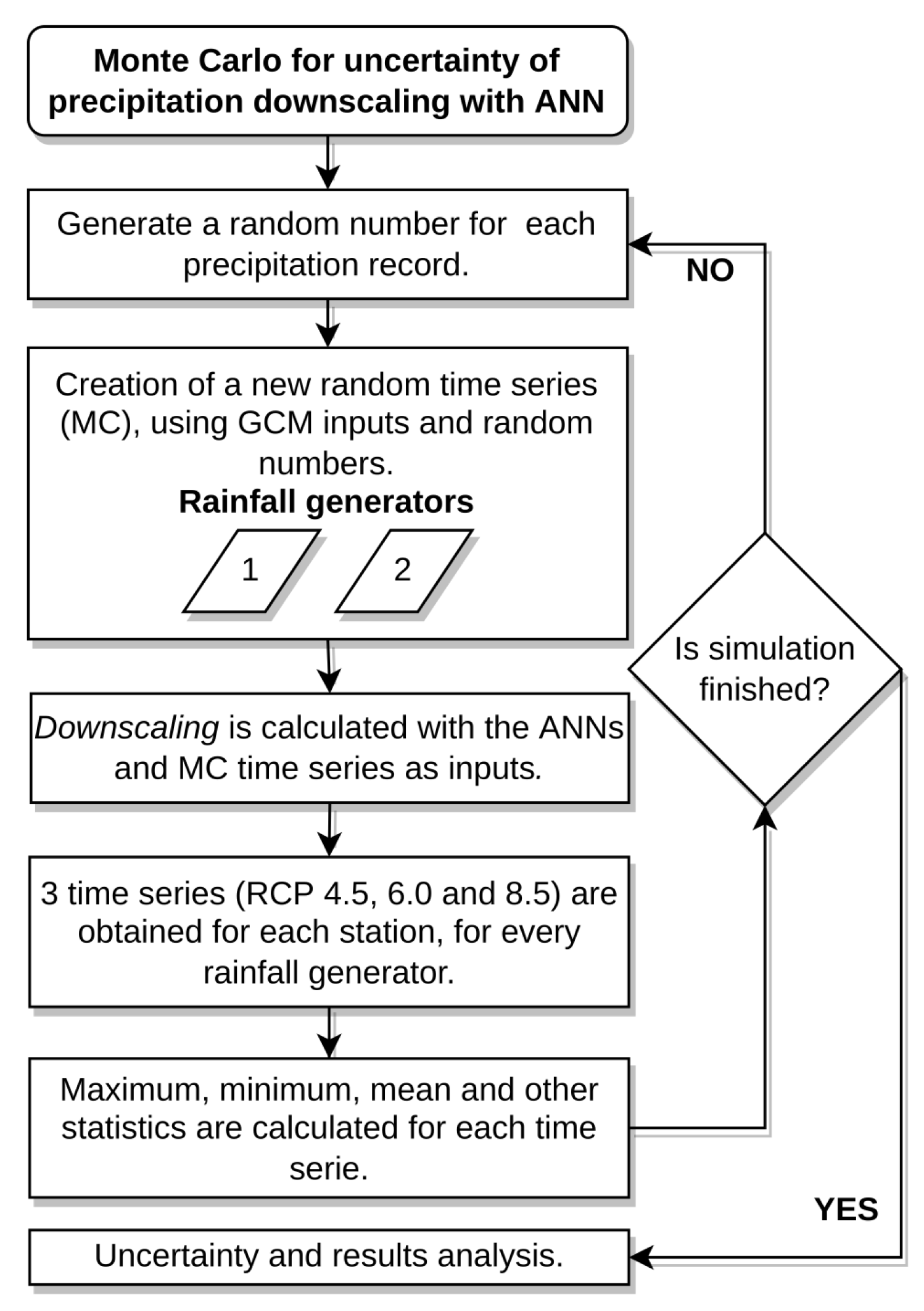
This paper proposes a Monte Carlo simulation, as shown in Figure 2, to estimate and control the uncertainty associated with the overall process. The proposal generates multiple random time series data from GCM projections, augmented by resampling.

Equations (5) and (6) show the case of using two rainfall generators to modify the input of the GCM rainfall time series. New Monte Carlo time series were created for each one. Particularly, Equation (5) represents the high uncertainty in rainfall inputs and (6) generates a similar time series to the GCM with a $\pm n$ of variation from the GCM,

$$G_{1i}=x_i\ast r_1,$$

(5)

$$G_{2i}=x_i+r_2,$$

(6)

where G is the random Monte Carlo precipitation for rainfall generators 1 and 2, $x_i$ is the GCM precipitation, $r_1$ is a random number generated between 0 and 1, $r_2$ is a random number generated in a range of $r_2\in [-n,n]$, and n is the uncertainty in the input precipitations to be tested.

The rainfall generators were applied to every precipitation record, changing the random number in each record to improve randomness. This process generates a new time series that is the input of the validated ANN. The structure of ANN is not modified in this process, so the generation of the downscaled time series is very fast. The procedure is replicated for each station and RCP4.5, RCP6.0, and RCP8.5 emission scenarios until the Monte Carlo process finishes (Figure 2).

3. Case Study

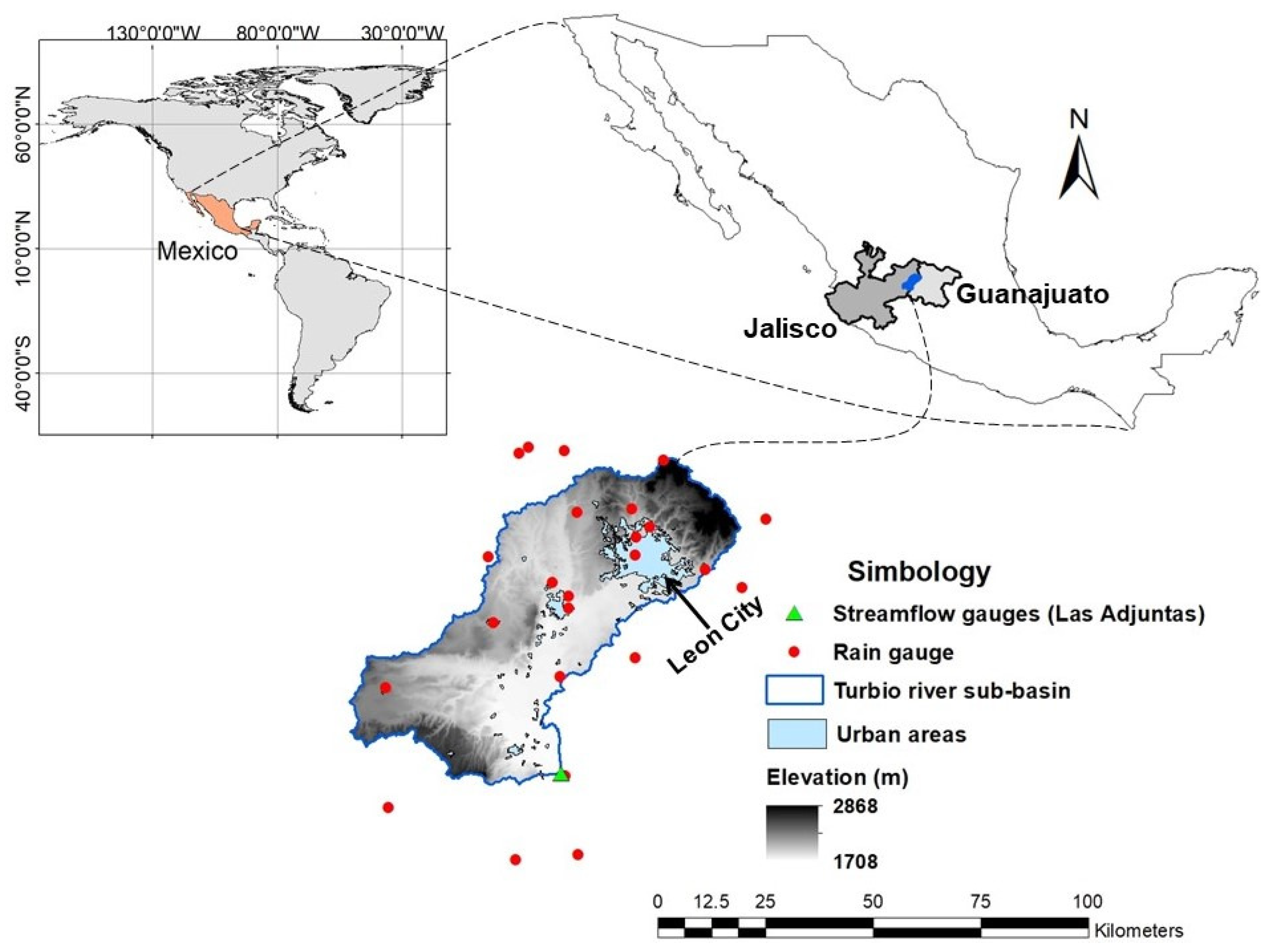
The Turbio River sub-basin is approximately located in the center of Mexico, as Figure 3 shows. This sub-basin is of particular relevance since it presented over-exploitation problems on the surface and groundwater in recent decades [30]. Overall, it is an important system for the country given its large agricultural and industrial production. In addition, the Turbio River sub-basin includes important urban areas. Figure 3 shows the case of Leon, a city with nearly 2 million inhabitants. Economic, industrial, and urban development significantly altered the ecosystems in the Turbio River sub-basin. Consequently, it has generated great uncertainty among decision-makers concerning the impact of climate change on future water, environmental, and socioeconomic aspects.

The sub-basin has an area of 2983 km² and is located between elevations 1708 and 2868 m. The accumulated average annual rainfall varies from 560 to 807 mm, with a very marked seasonality, peaking in the rainy season (June to September) with an occurrence of 90% of the annual rainfall. The mean variation of the minimum and maximum temperatures in the sub-basin is from 9.56 °C to 25.59 °C [30]. The particularly limited information at this sub-basin will allow for a better evaluation of the robustness of the proposed methodology.

Rainfall data were obtained from the National Weather Service (https://smn.conagua.gob.mx/es/ accessed on 8 February 2023) and we obtained the projections of the CMIP5 project GCMs from the Earth System Grid Federation (https://esgf-node.llnl.gov/projects/esgf-llnl/ accessed on 8 February 2023). In order to generate the downscaling, the inputs used to train and validate the ANN were the monthly rainfall obtained from the 24 meteorological stations (Figure 3) and the GCM projections. We used the monthly scale, so the seasonal tendency is clearly represented in the hydrological model; this study also focuses on the quantification of yearly water availability to estimate the vulnerabilities and feed the ANN with monthly data (to speed up the process of downscaling). The downscaling was computed for the period 1982–2006, considering the emission scenarios RCP4.5, RCP6.0, RCP8.5, and the projections of 13 GCM precipitation scenarios.

Hydrological modeling was conducted using the TETIS model (see [45,46] for more information about the TETIS model) and daily flow data were measured at the Las Adjuntas gauge, which is located at the mouth of the sub-basin (Figure 3). The flow data measured can be freely downloaded from the website of CONAGUA National Data Bank of Surface Waters (https://www.imta.gob.mx/bandas accessed on 8 February 2023). The calibration of the hydrological model was computed on a monthly scale using the flow data.

4. Results and Discussion

4.1. Hydrology Model Performance

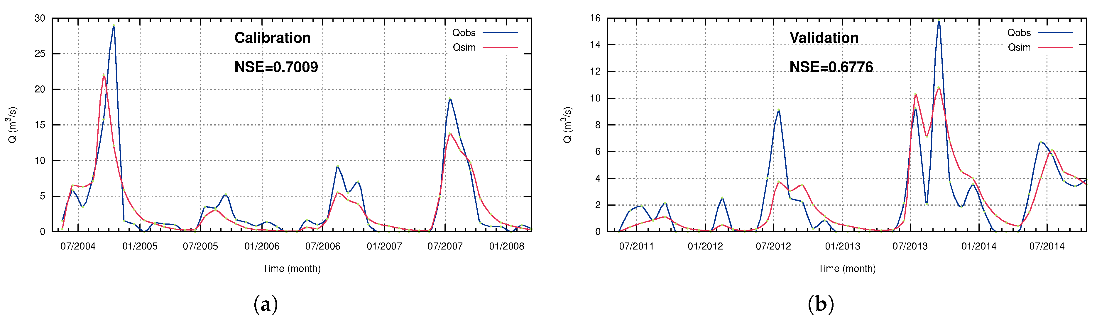
The selected calibration period ranged from May 2004 to March 2008. The NSE serves as the objective function of the hydrological model calibration [47] as it normalizes the model performance into an interpretable scale [48].

Table 2. Hydrological model’s effective mean parameters obtained by calibration.

Parameter	Correction Factor	Parameter Equation	Effective Parameter
Static storage	$F{C}_1$	$H_{u\left(i\right)}^{*}=F{C}_1·H_u$	382.090 (mm)
Vegetation cover index	$F{C}_2$	${\Lambda }^{*}=F{C}_2·{\lambda }_v$	0.008 $(-)$
Infiltration capacity	$F{C}_3$	$k_{s\left(i\right)}^{*}=F{C}_3·k_s$	113.981 (mmh−1)
Overland flow velocity	$F{C}_4$	$u_{\left(i\right)}^{*}=F{C}_4·u$	5.158 (ms−1)
Percolation capacity	$F{C}_5$	$k_{p\left(i\right)}^{*}=F{C}_5·k_p$	7.216 (mmh−1)
Interflow velocity	$F{C}_6$	$k_{ss\left(i\right)}^{*}=F{C}_6·k_{ss}$	124.17 (mmh−1)
Deep aquifer permeability	$F{C}_7$	$k_{ps\left(i\right)}^{*}=F{C}_7·k_s$	0.067 (mmh−1)
Connected aquifer permeability	$F{C}_8$	$k_{sa\left(i\right)}^{*}=F{C}_8·k_{ps}$	0.010 (mmh−1)
River channel velocity	$F{C}_9$	$v_{\left(t\right)}^{*}=F{C}_9·v_{\left(t\right)}$	0.031 (mms−1)

presents the average of the effective parameters resulting from the calibration process [45,46,49]. In terms of efficiency, Figure 4a shows that the model reaches a NSE of 0.70 for the calibration period. The model performance can be judged as satisfactory if the NSE > 0.5 for the watershed scale [50]. The validation process of the hydrological model uses the period from May 2011 to October 2014. Figure 4b shows the good performance of the model, with a NSE of 0.68 in extrapolating the flow estimation out of the calibration period.

4.2. GCM Models and Downscaling

According to the methodology, once the hydrological model was built, calibrated, and validated, downscaling was carried out with the ANN. From the 13 CMIP5 models shown in

Table 3. List of GCMs considered in the selection of the final model [30].

GCM Model	Country
BCC-CSM1	China
MIROC-ESM-CHEM MIROC-ESM MIROC5	Japan
CanESM2	Canada
CNRM-CM5	France
CSIRO-MK3-6	Australia
GFDL-CM3 GISS-E2-R	USA
HADGEM2-Es	United Kingdom
INM-CM4	Russia
MPI-ESM-LR	Germany
MRI-CGCM3	Japan
NCC-NorESM1	Norway
IPSL-CMA-LR	France

, the best GCM was selected [30]. We used only one GCM to reduce the complexity in the ANN structure, reduce computation time, and control ANN errors. For this, the Pearson correlations (R) are compared between measured and historical data from 13 GCM models. The control period ranges from 1982 to 2014. As a result of the comparison, the best correlation ($R>0.6$) was obtained with CSIRO-Mk3-6-0. Consequently, the analysis continues with the selection of the CSIRO-Mk3-6-0 model for the downscaling and climate projections.

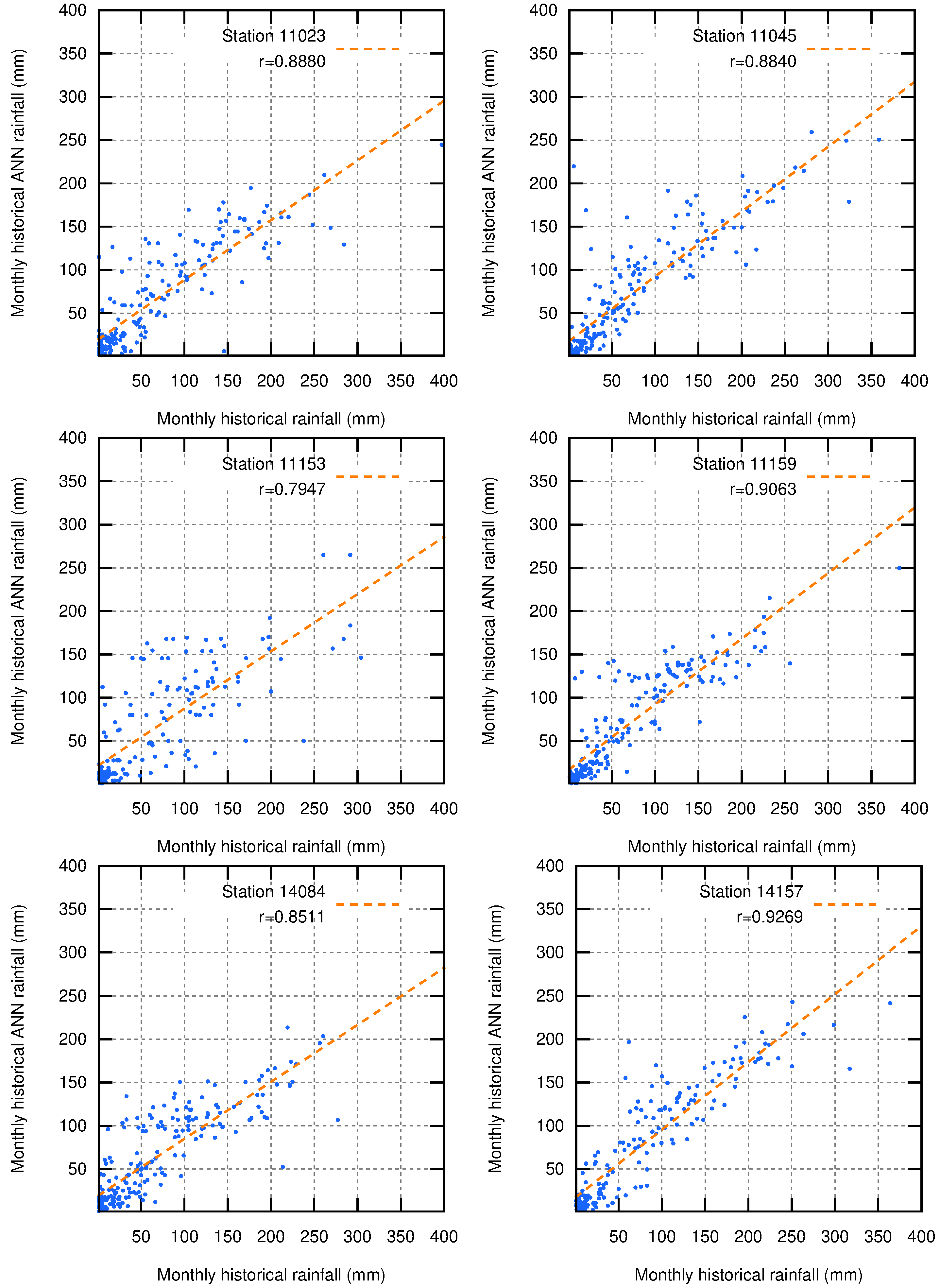
ANNs and CSIRO-Mk3-6-0 model projections for the RCP scenarios approached downscaling models for the daily data measured in the 24 rain gauges shown in Figure 3. The training period was confirmed by 24 years (1982–2014) for rainfall and 21 years (1982–2014) for evapotranspiration. The monthly rainfall was calculated from the daily observed and each station was trained individually. However, the model efficiency was considered as not good enough. To improve such a performance, the downscaling process used multiple combinations of information gathered at weather stations. The trained ANN had a total of 288 neurons in the hidden layer, which was equal to the months during the training period. The number of iterations was not limited and the average number of iterations required was 1500 for each ANN. The ANN training process was repeated until the convergence of the efficiency coefficients. The training results showed a maximum R equal to 0.92 as shown in Figure 5.

Downscaling with the ANNs managed to obtain a better fit to the measured rainfall data, and reduced the overestimation, this was confirmed with Monte Carlo (

Table 4. Comparison of average efficiency coefficients of CSIRO-Mk3-6-0 model and Monte Carlo downscaling for rainfall.

	CSIRO-Mk3-6-0	ANNs and Monte Carlo
		Minimum	Mean	Maximum
R	0.6156	0.6520	0.7121	0.7713
Bias	101.3	−4.9	2.0	9.1
Variance	13,538.2	3019.4	3430.2	3872.2
Underestimation	−39.5	−46.9	−40.7	−35.1
Overestimation	75.9	25.7	30.3	35.1
RMSE	100.2	43.8	48.6	53.1

) and projected precipitations (Figure 6). Hence, significant reductions in the training period (1982–2006) were observed at all the stations: RMSE varied at a range of 14 to 49.7, an F from 0.54 to 0.82, and a bias from −3.16% to 8.22%. In the case of evapotranspiration, the performance was acceptable, with an R of up to 0.82 and a bias between −1.06% and 0.08%.

The validation period was confirmed by 8 years (2006–2014) for precipitation, and 3 years (2003–2006) for evapotranspiration. For precipitation validation, climate change was considered and historical data were compared with RCP4.5, RCP6.0, and RCP8.5 emission scenarios. The results show a tendency for the ANNs to underestimate precipitations (Table 4 and

Table 5. Minimum, mean, and maximum coefficients of the monthly rainfall outputs for the Monte Carlo iterations, using random generator 2.

Rain Gauge		R	Bias	Variance	Underestimation	Overestimation	RMSE	Maximum	Mean
11,020	MIN	0.640	−6.0	2621.4	−44.8	24.0	44.9	176.7	46.3
	MEAN	0.695	0.6	3029.3	−39.3	28.6	49.5	205.9	49.5
	MAX	0.752	7.4	3425.3	−33.6	33.8	53.5	221.2	52.9
11,023	MIN	0.668	−5.6	2751.4	−47.0	25.7	41.3	217.0	50.1
	MEAN	0.730	1.7	3022.3	−39.4	29.1	45.8	241.0	53.2
	MAX	0.787	8.9	3302.2	−33.7	33.4	50.4	244.6	56.4
11,045	MIN	0.618	−13.2	3420.1	−52.4	26.8	49.8	206.4	50.0
	MEAN	0.689	−5.6	3972.4	−45.4	32.5	56.6	251.2	54.4
	MAX	0.764	2.4	4458.6	−40.2	38.2	62.2	259.2	59.0
11,049	MIN	0.600	−2.1	2818.6	−44.3	27.8	44.2	215.1	52.5
	MEAN	0.672	5.4	3342.4	−38.4	33.1	50.1	284.2	56.9
	MAX	0.745	12.9	3837.6	−32.3	39.5	55.7	371.9	60.9
11,159	MIN	0.715	−1.7	2881.8	−41.0	21.7	39.4	179.0	49.7
	MEAN	0.756	3.9	3179.6	−35.4	26.4	44.2	214.0	52.6
	MAX	0.809	9.1	3501.3	−30.9	29.8	47.6	249.7	55.2
14,083	MIN	0.405	−27.8	239.2	−23.3	8.3	22.0	65.4	13.9
	MEAN	0.539	−20.1	343.2	−20.5	10.4	24.7	131.0	15.2
	MAX	0.669	−9.4	501.5	−18.1	13.5	27.5	146.4	17.0

) in comparison to overestimation. However, ANNs maintain good efficiencies with coefficients ranging between 0.47 and 0.81. On the other hand, the model again underestimates evapotranspiration; downscaling with the ANNs achieves an average R of 0.52.

4.3. Uncertainty Analysis and Projections

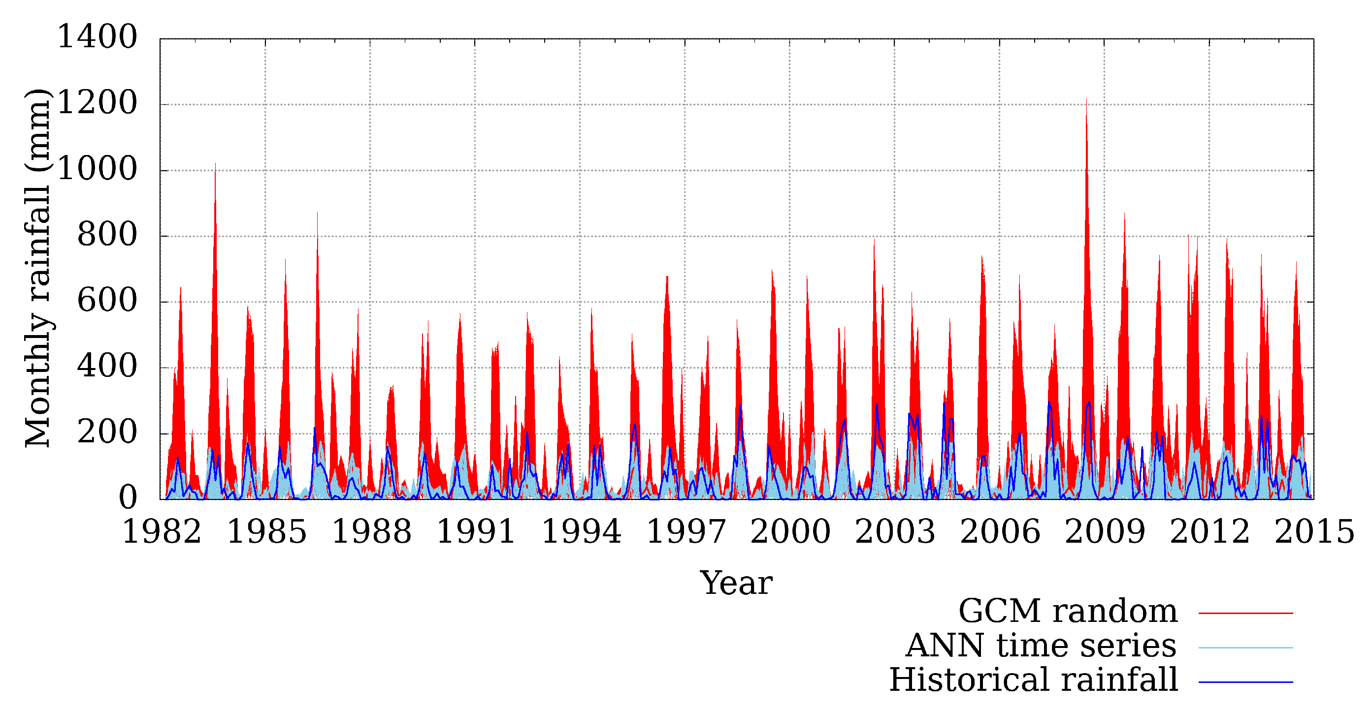
We evaluated the uncertainty associated with precipitation and evapotranspiration projections because previous research has shown that these projections have significant uncertainties associated with them [17]. However, we considered that it was essential for future research to include the uncertainty associated with the other components showcased by the methodology presented here. The evaluation period was from 1982 to 2015. Figure 7 and Figure 8 show the time series of a 1000-iteration Monte Carlo simulation calculated using random generator 1 from Equation (5), and random generator 2 from Equation (6). The Monte Carlo time series generated with Equation (5) has a bias between 55% and 115%. This interval shrunk to 82% and 90%, given Equation (6). Generator number 1 represents the highest uncertainty with a bias of the ANN time series between −10% and 4%. The bias calculated using generator number 2 is between −6% and 9%. Similar behaviors were observed with the RMSE coefficients for the other stations. Generator number 2 reduces the errors across the simulation in most of the cases (Table 5). These results prove that the error was reduced by at least three times when using ANN downscaling.

Underestimation/overestimation and maximum precipitation were calculated for each time series. The maximum value is always reached at different fixed points at every station and ANN does not predict the rainfall above that value. Overall, the average overestimation of all stations is 30.3 mm, while the average underestimation is 40.7 mm for generator number 2 with a proposed input uncertainty of ±15 mm. In contrast, generator number 1 estimates an overestimation of 28.8 mm and an underestimation of 47.7 mm. As a result of the proposed methodology, the ANN-combined approach reduces the overestimation by 60% in comparison to the CSIRO-Mk3-6-0 model and there is an underestimation of −5 mm in the average of the overall stations when using ANN downscaling (Table 4). RMSE and variance confirm the results. However, the underestimations of all stations did not improve as expected with the ANN-combined methodology and, in most cases, it remained at a similar level when compared to directly using the GCM model.

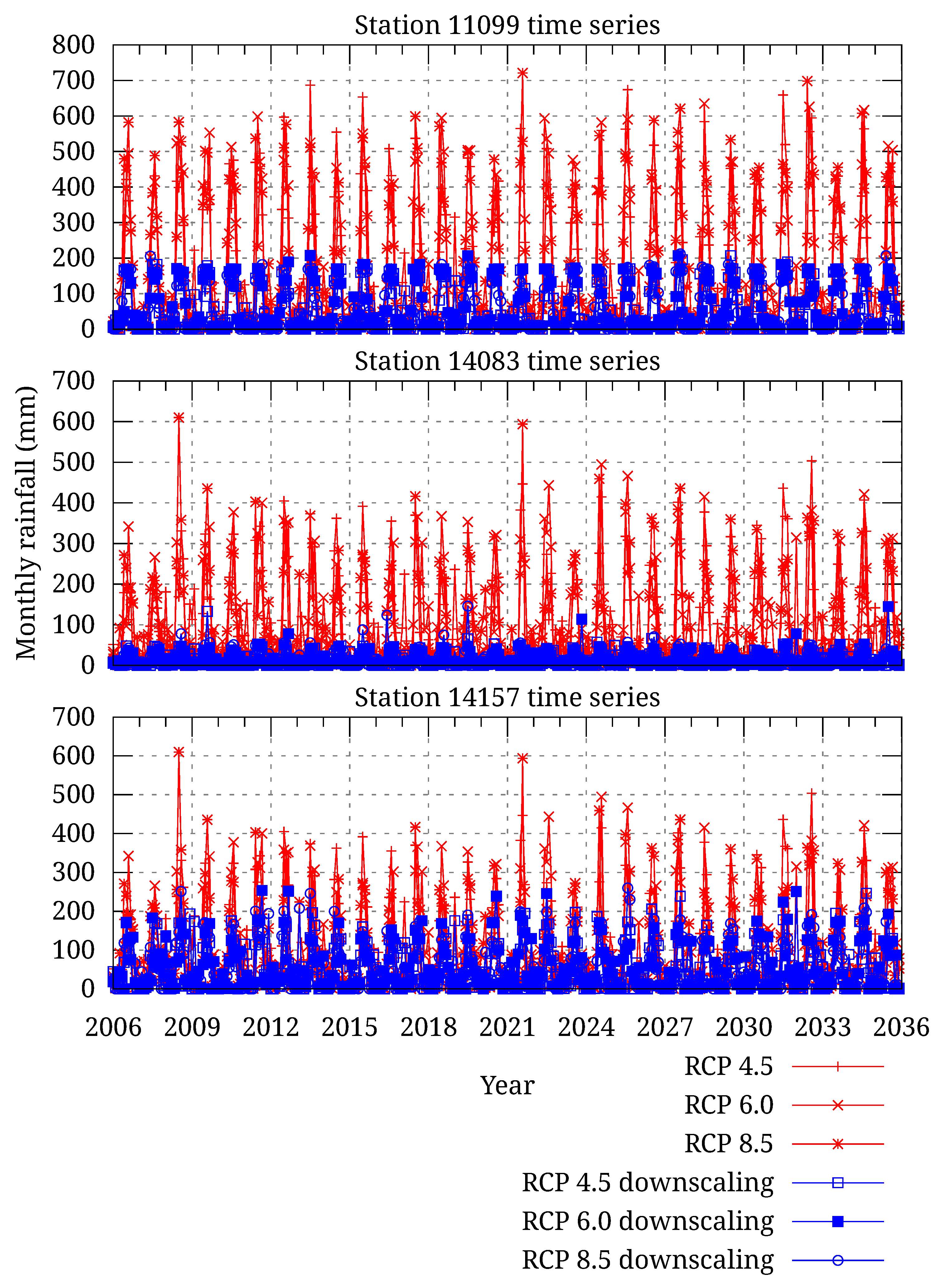
Finally, monthly climate projections using ANNs for the RCP4.5, RCP6.0, and RCP8.5 emission scenarios were generated for precipitation and evapotranspiration from 2015 to 2035. We only evaluated in the previous period (near future, the year 2035) to counteract the increased uncertainties of climate projections and achieve a better interpretation of the performances of the ANNs. However, it is important to continue investigating how the ANN performances behave when projecting into the distant future. Figure 6 and Figure 9 show the results of the projections using the ANNs. In both, it can be seen that the projections follow the same trends as in the training and validation for each rain gauge. We observed few changes over time; ANN corrects the overestimates of precipitation and the underestimates of evapotranspiration.

4.4. Vulnerability to Climate Change Impacts

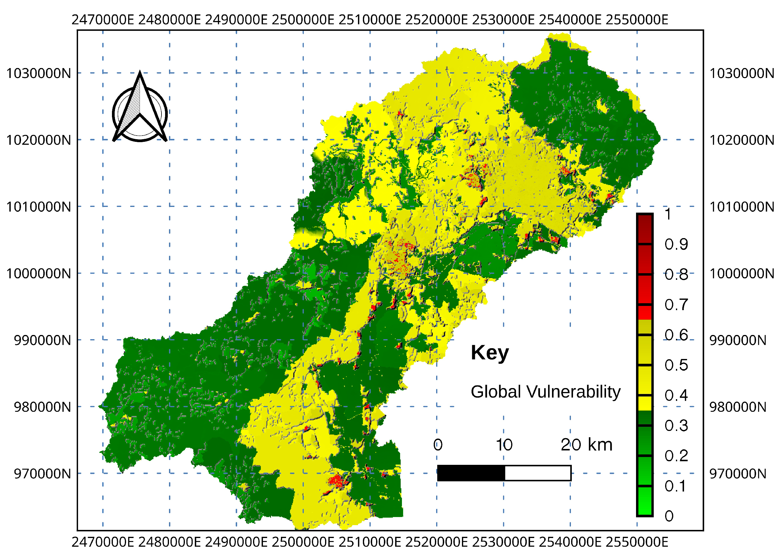
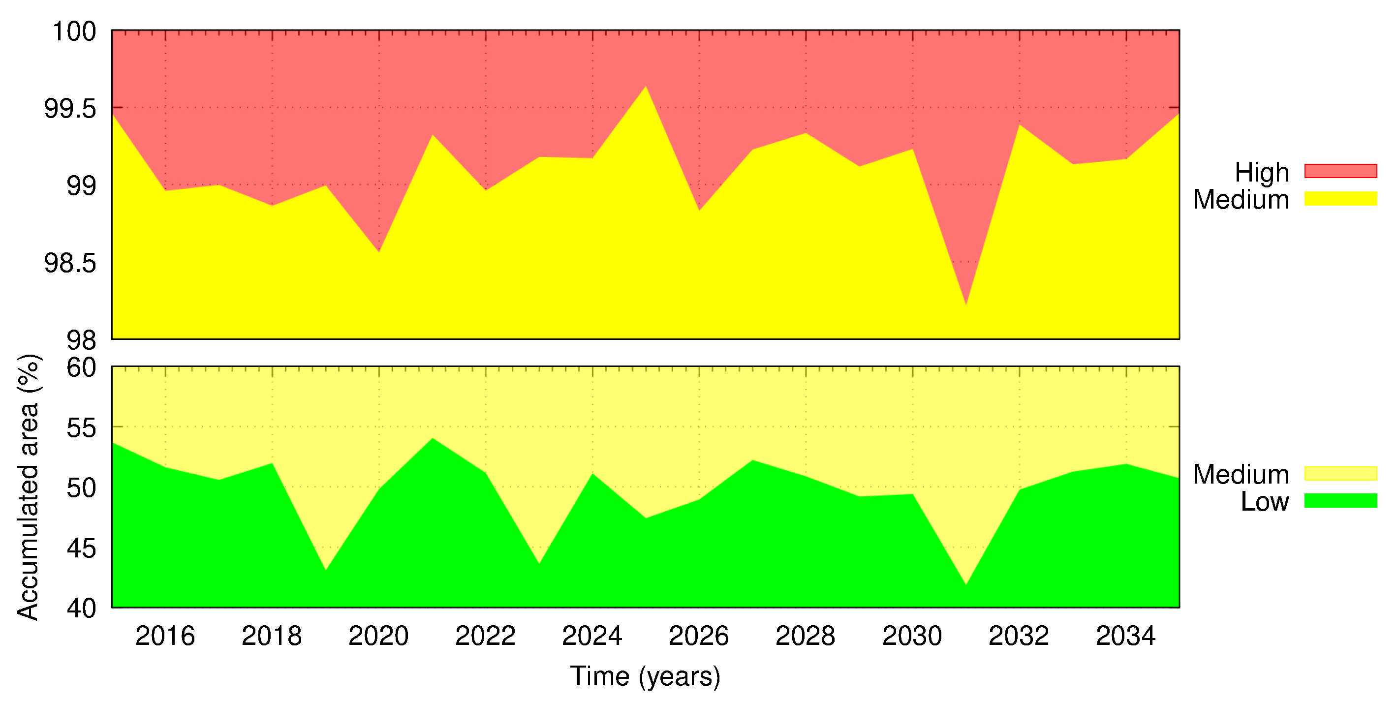
The current and future sub-basin water and environmental vulnerabilities were quantified and the social and economic sectors were added on top. The final result is the global vulnerability to the effects of climate change on precipitation and evapotranspiration considering the accumulated effects over the sectors. This process was done with the MPDV2.0 model for the years 2014 to 2035. MPDV2.0 classifies the vulnerability as low vulnerability (0 ≤ indices ≤ 0.35), medium vulnerability (0.36 ≤ indices ≤ 0.65), and high vulnerability (0.66 ≤ indices ≤ 1.0). Considering the uncertainty associated with the projections of the ANNs and CSIRO-Mk3-6-0 model, the results show that 51.2% of the area of the sub-basin represents low vulnerability, 47.8% represents medium vulnerability, and only 1% represents high vulnerability (Figure 10). The highest vulnerabilities usually occur in an urban environment, followed by agricultural areas (Figure 10). We can also observe that the sub-basin presents the lowest vulnerabilities in the protected areas, considering the great importance of conserving these natural habitats. The vulnerability shows insignificant increases in the near future, as could be expected, considering that in the three scenarios, there is no immediate action to further reduce greenhouse gas emissions than considering the uncertainty associated with the GCM projections for the RCP4.5, RCP6.0, and RCP8.5 emission scenarios. However, increases in the areas with high vulnerability are observed for the three RCP scenarios. For instance, the RCP6.0 scenario presents areas with medium vulnerability that were reduced and became high in the year 2031, as Figure 11 shows. It can also be seen that the largest increments in the area occupied by high vulnerability for each scenario were: RCP4.5 (0.83%, year 2023), RCP6.0 (1.01%, year 2031), y RCP8.5 (1.31%, year 2022). Consequently, the RCP8.5 emission scenario produces the greatest increments in vulnerability, which is the most extreme scenario. A comparison of the figures shows that the more extreme the RCP scenario, the more pronounced the changes in vulnerability.

The vulnerabilities of 2015, 2022, 2023, 2031, and 2035 are identified as critical for each RCP scenario. The first three years present similar spatial vulnerability distributions, mainly for the RCP4.0 and RCP6.0 emission scenarios. In 2023, the highest vulnerabilities increased by 0.83% in the RCP4.5 scenario; for RCP8.5 a decrease of 1.03% was observed. The year 2031 presented the greatest vulnerabilities for the sub-basin, and the RCP6.0 scenario had the highest rates (Figure 11). We observe a similar spatial distribution for 2035, where projected rainfall has very important influence. The assessment shows that the global vulnerability in a sub-basin region has high spatial and temporal variability. Hence, the area occupied by high vulnerability increases considerably in the next year, while it almost disappears in the following year.

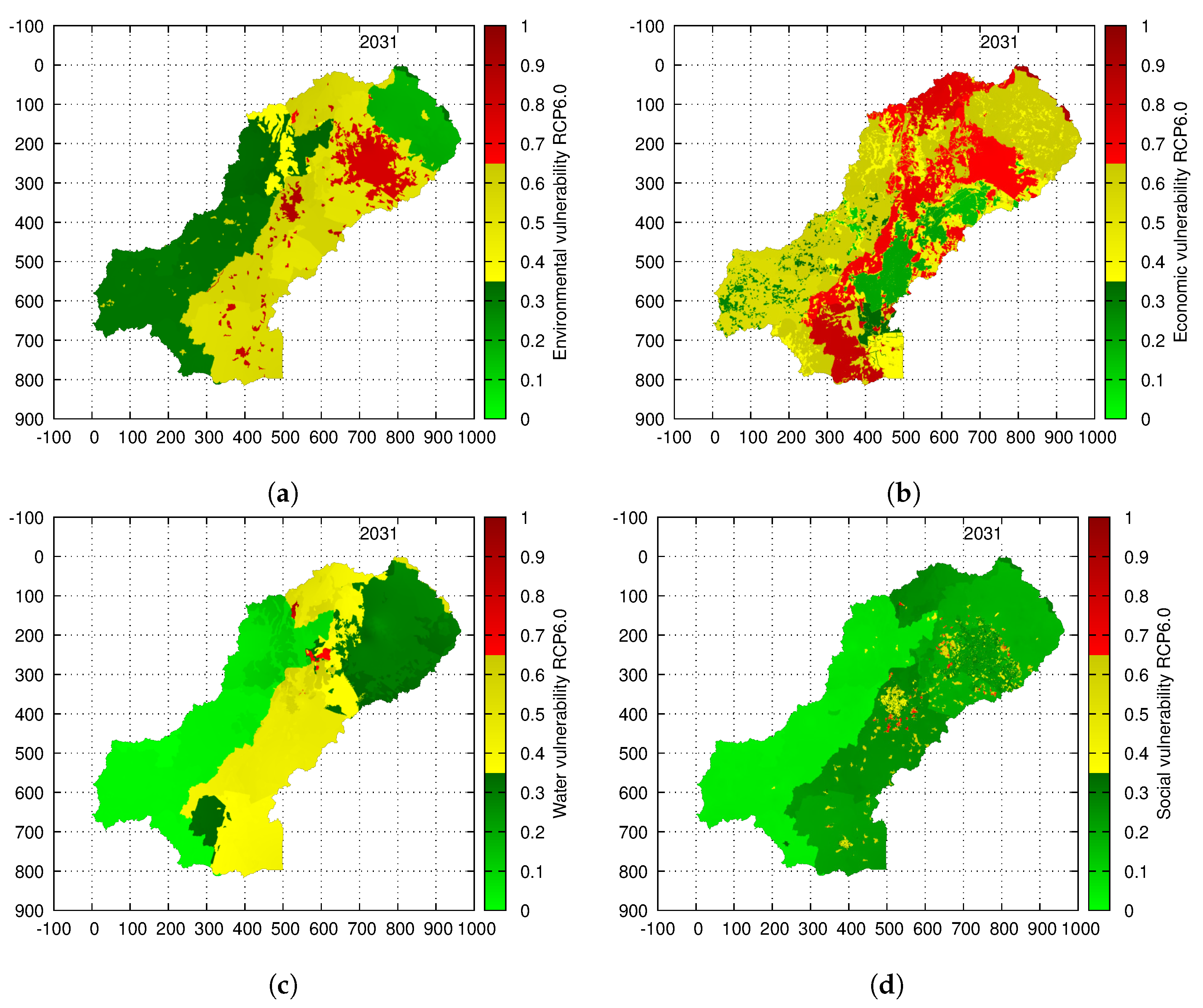
The environmental, socioeconomic, and water vulnerability evaluations allow us to estimate a global vision of vulnerability and determine the vulnerability particularly focused on the hydrological system. To carry this out, five vulnerability maps were generated for each year in the period from 2014 to 2035 (22 years). That is a total of 110 different maps for each RCP emission scenario. In addition, the change in the area occupied by each type of vulnerability was calculated to evaluate the differences between 2014 and 2031. In 2031, high vulnerability presented a 10% increase in economic vulnerability. Figure 12 shows that the greatest change occurred in the water vulnerability to climate change, less than a 21% of the area occupied by low vulnerability became medium vulnerability.

5. Conclusions

The main proposal of this paper revolves around the combination of distributed hydrological models and ANNs for assessing the evolution of spatially distributed indicators on the impacts of climate change in river basin areas. One of the main novelties of the current proposal is the use of a Monte Carlo simulation method to assess the uncertainty of the process, particularly the uncertainty associated with a GCM downscaling process that is not captured, in principle, by the ANN model.

The results obtained with the coupled MPDV2.0 model show that the 48.8% Turbio River sub-basin already presents medium and high vulnerability areas at the current climatic conditions, specifically in agricultural and urban areas. In addition, increases in medium and high vulnerabilities are projected for the near future, particularly in the aforementioned areas. Based on the current conditions, an increase of 9.3% in medium and highly vulnerable areas is projected for the year 2031. Above all, a significant increase in water and environmental vulnerability is projected due to the decrease in precipitation and a significant increase in evapotranspiration. The projections of precipitation with the ANNs and the CSIRO-Mk3-6-0 model present an uncertainty of 15 mm per month.

The uncertainty associated with the projections suggests that it will be necessary to continue the estimation and control of the watershed vulnerabilities in the long term. The recommendation is to evaluate the model in future intervals of five or ten years; this period is necessary for public organizations to obtain the required social, economic, and environmental data. Then the model should be updated, analyzing how the reality and the models behave and projecting it again under the corrections made and the latest data.

For this particular case study, the climate information was analyzed on a monthly time scale, while the social and economic information and the final vulnerabilities had an annual scale, so one of the disadvantages of the methodology is that the vulnerability time scale is set by the longest scale. In addition, the Monte Carlo simulation requires a large amount of computational resources to calculate each iteration and the data created in each random scenario should be analyzed. For this, future research will focus on the in-depth analysis on the use of computational statistical methods to improve the efficiency of the overall process.

References

- Green, T.R.; Taniguchi, M.; Kooi, H.; Gurdak, J.J.; Allen, D.M.; Hiscock, K.M.; Treidel, H.; Aureli, A. Beneath the surface of global change: Impacts of climate change on groundwater. J. Hydrol. 2011, 405, 532–560. [Google Scholar] [CrossRef]
- Lizarralde, G.; Bornstein, L.; Robertson, M.; Gould, K.; Herazo, B.; Petter, A.M.; Páez, H.; Díaz, J.H.; Olivera, A.; González, G.; et al. Does climate change cause disasters? How citizens, academics, and leaders explain climate-related risk and disasters in Latin America and the Caribbean. Int. J. Disaster Risk Reduct. 2021, 58, 102173. [Google Scholar] [CrossRef]
- Herrera, M.; Ferreira, A.A.; Coley, D.A.; De Aquino, R.R. SAX-quantile based multiresolution approach for finding heatwave events in summer temperature time series. AI Commun. 2016, 29, 725–732. [Google Scholar] [CrossRef]
- Hewitson, B.C.; Crane, R.G. Consensus between GCM climate change projections with empirical downscaling: Precipitation downscaling over South Africa. Int. J. Climatol. 2006, 26, 1315–1337. [Google Scholar] [CrossRef]
- Chung, E.S.; Park, K.; Lee, K.S. The relative impacts of climate change and urbanization on the hydrological response of a Korean urban watershed. Hydrol. Process. 2011, 25, 544–560. [Google Scholar] [CrossRef]
- Jun, K.S.; Chung, E.S.; Sung, J.Y.; Lee, K.S. Development of spatial water resources vulnerability index considering climate change impacts. Sci. Total. Environ. 2011, 409, 5228–5242. [Google Scholar] [CrossRef] [PubMed]
- Tulbure, M.G.; Broich, M. Spatiotemporal patterns and effects of climate and land use on surface water extent dynamics in a dryland region with three decades of Landsat satellite data. Sci. Total Environ. 2019, 658, 1574–1585. [Google Scholar] [CrossRef]
- Wiréhn, L.; Danielsson, Å.; Neset, T.S.S. Assessment of composite index methods for agricultural vulnerability to climate change. J. Environ. Manag. 2015, 156, 70–80. [Google Scholar] [CrossRef]
- Boy-Roura, M.; Nolan, B.T.; Menció, A.; Mas-Pla, J. Regression model for aquifer vulnerability assessment of nitrate pollution in the Osona region (NE Spain). J. Hydrol. 2013, 505, 150–162. [Google Scholar] [CrossRef]
- Abson, D.J.; Dougill, A.J.; Stringer, L.C. Using Principal Component Analysis for information-rich socio-ecological vulnerability mapping in Southern Africa. Appl. Geogr. 2012, 35, 515–524. [Google Scholar] [CrossRef]
- Cheng, J.; Ping Tao, J. Fuzzy Comprehensive Evaluation of Drought Vulnerability Based on the Analytic Hierarchy Process—An Empirical Study from Xiaogan City in Hubei Province. Agric. Agric. Sci. Procedia 2010, 1, 126–135. [Google Scholar] [CrossRef]
- Maiolo, M.; Martirano, G.; Morrone, P.; Pantusa, D. Assessment criteria for a sustainable management of the water resources. Water Pract. Technol. 2006, 1, wpt2006012. [Google Scholar] [CrossRef]
- Tixier, J.; Dandrieux, A.; Dusserre, G.; Bubbico, R.; Mazzarotta, B.; Silvetti, B.; Hubert, E.; Rodrigues, N.; Salvi, O. Environmental vulnerability assessment in the vicinity of an industrial site in the frame of ARAMIS European project. J. Hazard. Mater. 2006, 130, 251–264. [Google Scholar] [CrossRef] [PubMed]
- Brody, S.D.; Zahran, S.; Vedlitz, A.; Grover, H. Examining the Relationship Between Physical Vulnerability and Public Perceptions of Global Climate Change in the United States. Environ. Behav. 2008, 40, 72–95. [Google Scholar] [CrossRef]
- Dixon, B. Applicability of neuro-fuzzy techniques in predicting ground-water vulnerability: A GIS-based sensitivity analysis. J. Hydrol. 2005, 309, 17–38. [Google Scholar] [CrossRef]
- Cess, R.D.; Potter, G.L.; Blanchet, J.P.; Boer, G.J.; Del Genio, A.D.; Déqué, M.; Dymnikov, V.; Galin, V.; Gates, W.L.; Ghan, S.J.; et al. Intercomparison and interpretation of climate feedback processes in 19 atmospheric general circulation models. J. Geophys. Res. Atmos. 1990, 95, 16601–16615. [Google Scholar] [CrossRef]
- Song, Y.H.; Chung, E.S.; Shahid, S. Spatiotemporal differences and uncertainties in projections of precipitation and temperature in South Korea from CMIP6 and CMIP5 general circulation models. Int. J. Climatol. 2021, 41, 5899–5919. [Google Scholar] [CrossRef]
- Ali, S.; Eum, H.I.; Cho, J.; Dan, L.; Khan, F.; Dairaku, K.; Shrestha, M.L.; Hwang, S.; Nasim, W.; Khan, I.A.; et al. Assessment of climate extremes in future projections downscaled by multiple statistical downscaling methods over Pakistan. Atmos. Res. 2019, 222, 114–133. [Google Scholar] [CrossRef]
- Samanta, S.; Banerjee, S.; Patra, P.K.; Sehgal, V.K.; Chowdhury, A.; Kumar, B.; Mukherjee, A. Projection of future daily global horizontal irradiance under four RCP scenarios: An assessment through newly developed temperature and rainfall-based empirical model. Sol. Energy 2021, 227, 23–43. [Google Scholar] [CrossRef]
- Wilby, R.; Wigley, T. Downscaling general circulation model output: A review of methods and limitations. Prog. Phys. Geogr. Earth Environ. 1997, 21, 530–548. [Google Scholar] [CrossRef] [Green Version]
- Wang, J.; Nathan, R.; Horne, A.; Peel, M.C.; Wei, Y.; Langford, J. Evaluating four downscaling methods for assessment of climate change impact on ecological indicators. Environ. Model. Softw. 2017, 96, 68–82. [Google Scholar] [CrossRef]
- Govindaraju, R.S.; Rao, A.R. Artificial Neural Networks in Hydrology; Springer Science & Business Media: Berlin/Heidelberg, Germany, 2013; Volume 36. [Google Scholar]
- Tiwari, M.K.; Chatterjee, C. Uncertainty assessment and ensemble flood forecasting using bootstrap based artificial neural networks (BANNs). J. Hydrol. 2010, 382, 20–33. [Google Scholar] [CrossRef]
- Gaume, E.; Gosset, R. Over-parameterisation, a major obstacle to the use of artificial neural networks in hydrology? Hydrol. Earth Syst. Sci. 2003, 7, 693–706. [Google Scholar] [CrossRef]
- Ajami, N.K.; Duan, Q.; Gao, X.; Sorooshian, S. Multimodel Combination Techniques for Analysis of Hydrological Simulations: Application to Distributed Model Intercomparison Project Results. J. Hydrometeorol. 2006, 7, 755–768. [Google Scholar] [CrossRef]
- Dixon, B.; Earls, J. Effects of urbanization on streamflow using SWAT with real and simulated meteorological data. Appl. Geogr. 2012, 35, 174–190. [Google Scholar] [CrossRef]
- Tegegne, G.; Kim, Y.O.; Seo, S.B.; Kim, Y. Hydrological modeling uncertainty analysis for different flow quantiles: A case study in two hydro-geographically different watersheds. Hydrol. Sci. J. 2019, 64, 473–489. [Google Scholar] [CrossRef]
- McMillan, H.K.; Westerberg, I.K.; Krueger, T. Hydrological data uncertainty and its implications. WIREs Water 2018, 5, e1319. [Google Scholar] [CrossRef]
- Pechlivanidis, I.; Jackson, B.; Mcintyre, N.; Wheater, H. Catchment scale hydrological modeling: A review of model types, calibration approaches and uncertainty analysis methods in the context of recent developments in technology and applications. Glob. NEST J. 2011, 13, 193–214. [Google Scholar]
- Orozco, I.; Martínez, A.; Ortega, V. Assessment of the Water, Environmental, Economic and Social Vulnerability of a Watershed to the Potential Effects of Climate Change and Land Use Change. Water 2020, 12, 1682. [Google Scholar] [CrossRef]
- Das, J.; Nanduri, U.V. Assessment and evaluation of potential climate change impact on monsoon flows using machine learning technique over Wainganga River basin, India. Hydrol. Sci. J. 2018, 63, 1020–1046. [Google Scholar] [CrossRef]
- Fazeli Farsani, I.; Farzaneh, M.R.; Besalatpour, A.A.; Salehi, M.H.; Faramarzi, M. Assessment of the impact of climate change on spatiotemporal variability of blue and green water resources under CMIP3 and CMIP5 models in a highly mountainous watershed. Theor. Appl. Climatol. 2019, 136, 169–184. [Google Scholar] [CrossRef]
- Harrison, P.A.; Dunford, R.W.; Holman, I.P.; Cojocaru, G.; Madsen, M.S.; Chen, P.Y.; Pedde, S.; Sandars, D. Differences between low-end and high-end climate change impacts in Europe across multiple sectors. Reg. Environ. Chang. 2019, 19, 695–709. [Google Scholar] [CrossRef]
- Wilson, K.; Newton, A.; Echeverría, C.; Weston, C.; Burgman, M. A vulnerability analysis of the temperate forests of south central Chile. Biol. Conserv. 2005, 122, 9–21. [Google Scholar] [CrossRef]
- Wang, X.; Zhong, X.; Liu, S.; Liu, J.; Wang, Z.; Li, M. Regional assessment of environmental vulnerability in the Tibetan Plateau: Development and application of a new method. J. Arid. Environ. 2008, 72, 1929–1939. [Google Scholar] [CrossRef]
- Enea, M.; Salemi, G. Fuzzy approach to the environmental impact evaluation. Ecol. Model. 2001, 136, 131–147. [Google Scholar] [CrossRef]
- Nandy, S.; Singh, C.; Das, K.; Kingma, N.; Kushwaha, S. Environmental vulnerability assessment of eco-development zone of Great Himalayan National Park, Himachal Pradesh, India. Ecol. Indic. 2015, 57, 182–195. [Google Scholar] [CrossRef]
- Field, C.B.; Barros, V.; Stocker, T.F.; Dahe, Q. Managing the Risks of Extreme Events and Disasters to Advance Climate Change Adaptation: Special Report of the Intergovernmental Panel on Climate Change; Cambridge University Press: Cambridge, UK, 2012. [Google Scholar] [CrossRef]
- Ortega-Gaucin, D.; Cruz, J.; Castellano Bahena, H. Peligro, vulnerabilidad y riesgo por sequía en el contexto del cambio climático en México. In Agua y Cambio Climático, 1st ed.; Lobato, R., Pérez, A.A., Eds.; Instituto Mexicano de Tecnología del Agua: Jiutepec, Mexico, 2018; pp. 78–103. [Google Scholar]
- Neelin, J.D.; Langenbrunner, B.; Meyerson, J.E.; Hall, A.; Berg, N. California Winter Precipitation Change under Global Warming in the Coupled Model Intercomparison Project Phase 5 Ensemble. J. Clim. 2013, 26, 6238–6256. [Google Scholar] [CrossRef]
- Montenegro, D.D.; Pérez Ortiz, M.A.; Vargas Franco, V.; Franco, V.V. Predicción de precipitación mensual mediante Redes Neuronales Artificiales para la cuenca del río Cali, Colombia. DYNA 2019, 86, 122–130. [Google Scholar] [CrossRef]
- Nourani, V.; Jabbarian Paknezhad, N.; Sharghi, E.; Khosravi, A. Estimation of prediction interval in ANN-based multi-GCMs downscaling of hydro-climatologic parameters. J. Hydrol. 2019, 579, 124226. [Google Scholar] [CrossRef]
- Okkan, U.; Kirdemir, U. Downscaling of monthly precipitation using CMIP5 climate models operated under RCPs. Meteorol. Appl. 2016, 23, 514–528. [Google Scholar] [CrossRef] [Green Version]
- Lorrentz, P. Artificial Neural Systems: Principle and Practice; Bentham Science Publishers: Sharjah, United Arab Emirates, 2015. [Google Scholar]
- Orozco, I.; Francés, F.; Mora, J. Parsimonious Modeling of Snow Accumulation and Snowmelt Processes in High Mountain Basins. Water 2019, 11, 1288. [Google Scholar] [CrossRef]
- Francés, F.; Vélez, J.I.; Vélez, J.J. Split-parameter structure for the automatic calibration of distributed hydrological models. J. Hydrol. 2007, 332, 226–240. [Google Scholar] [CrossRef]
- Bauwe, A.; Eckhardt, K.U.; Lennartz, B. Predicting dissolved reactive phosphorus in tile-drained catchments using a modified SWAT model. Ecohydrol. Hydrobiol. 2019, 19, 198–209. [Google Scholar] [CrossRef]
- Knoben, W.J.M.; Freer, J.E.; Woods, R.A. Technical note: Inherent benchmark or not? Comparing Nash—Sutcliffe and Kling–Gupta efficiency scores. Hydrol. Earth Syst. Sci. 2019, 23, 4323–4331. [Google Scholar] [CrossRef]
- Ruiz-Pérez, G.; González-Sanchis, M.; Campo, A.D.; Francés, F. Can a parsimonious model implemented with satellite data be used for modeling the vegetation dynamics and water cycle in water-controlled environments? Ecol. Model. 2016, 324, 45–53. [Google Scholar] [CrossRef] [Green Version]
- Moriasi, D.N.; Gitau, M.W.; Pai, N.; Daggupati, P. Hydrologic and water quality models: Performance measures and evaluation criteria. Trans. ASABE 2015, 58, 1763–1785. [Google Scholar]
Figure 1.
Conceptual scheme of the assessment of present and future vulnerabilities, executed in MPDV2.0.
Figure 2.
Monte Carlo methodology.
Figure 3.
Location of the Turbio River sub-basin used as a study area including the rain gauges (°) and stream-flow gauge (Δ).
Figure 4.
Efficiencies of hydrological modeling in (a) the calibration period and (b) the validation (− Qobs = measure discharge and • Qsim = simulated discharge).
Figure 5.
Examples of correlations (R) showing the efficiency obtained by the ANNs in the training period.
Figure 6.
Projected precipitation using ANNs and the CSIRO-Mk3-6-0 model.
Figure 7.
Results of the Monte Carlo simulation for random generator 2 (rain gauge: 11,020).
Figure 8.
Results of Monte Carlo simulation for random generator 1 (rain gauge: 11,020).
Figure 9.
Projected evapotranspiration using ANNs and the CSIRO-Mk3-6-0 model.
Figure 10.
Global vulnerability indices in the Turbio River sub-basin (year 2022, RCP6.0).
Figure 11.
Cumulative area distribution occupied by the global vulnerability for the RCP6.0 (years 2015 to 2035).
Figure 12.
Environmental (a), economic (b), hydrological (c), and social (d) vulnerability indices for the year 2031 (RCP6.0).