Third-Monthly Hydropower Scheduling of Cascaded Reservoirs Using Successive Quadratic Programming in Trust Corridor

Abstract

The third-monthly (about 10 days in a time-step) hydropower scheduling, typically a challenging nonlinear optimization, is one of the essential tasks in a power system with operational storage hydropower reservoirs. This work formulates the problem into quadratic programming (QP), which is solved successively, with the linearization updated on the nonlinear constraint of the firm hydropower yield from all the cascaded hydropower reservoirs. Notably, the generating discharge is linearly concaved with two planes, and the hydropower output is defined as a quadratic function of reservoir storage, release, and generating discharge. The application of the model and methods to four cascaded hydropower reservoirs on the Jinsha River reveals several things: the successive quadratic programming (SQP) presented in this work can derive results consistent with those by the dynamic programming (DP), typically with the difference in water level within 0.01m; it has fast convergence and computational time increasing linearly as the number of reservoirs increases, with the most significant improvement in the objective at the second iteration by about 20%; and it is capable of coordinating the cascaded reservoir very well to sequentially maximize the firm hydropower yield and the total hydropower production.

1. Introduction

Seasonal or monthly hydropower scheduling is one of the essential tasks in a power system with operational storage hydropower reservoirs. As shown by Allen and Bridgeman (1986), a seasonal load dispatch problem could be formulated to provide a preliminary evaluation of the ability of hydropower reservoirs to revise their system operation to maximize potential savings [1]. Wang et al. (2015) employed a monthly scheduling model to analyze the compensation benefits of four hydropower stations on the Jinsha River, which coordinate to reduce spillages during flood seasons and improve generation efficiency in dry seasons [2]. A deterministic monthly hydropower scheduling can also be simulated over many years of historical inflows in an implicit stochastic optimization to derive the operational rule of a reservoir [3]. Zambelli et al. (2011) demonstrated that an operational strategy based on deterministic modeling, when appropriately applied, can achieve similar performance to that which is yielded with a stochastic approach [4].

The monthly hydropower scheduling is typically a nonlinear optimization where the nonlinearity imposes challenges for a method to deliver an efficient solution; in addition, it is a problem in high dimensions when involving many operational storage reservoirs. The nonlinearity mainly comes from the hydropower output, a nonlinear function of the water head and generating discharge, and the generating capacity, which is also a nonlinear function of the water head [5,6].

Dynamic programming (DP), well known as one of the most applied mathematical optimization methods, effectively derives the global optimum at a discrete precision by transforming a multi-stage problem into multiple single-stage problems. However, it still encounters the “dimensional difficulty” [7] when dealing with a reservoir system on a large scale and at a high discretization resolution. Many strategies were proposed to improve its solution efficiency, including the DDDP [8,9], POA [10,11], and DPSA [12], which reduce the number of trials by using iterative ways to approach the optimum and are sensitive to the initial solution. In some cases, the problem of “dimensional difficulty” can somehow be alleviated by using the metaheuristic algorithms, such as Genetic Algorithm [13], Differential Evolution [14], Artificial Neural Networks [15,16], Particle Swarm Optimization [17,18,19], and Ant Colony Optimization [2], which, however, all have difficulty dealing with complex constraints, are sensitive to specific problems, and are inconsistent in securing the optimum. The fact that one of the extreme points is the optimum to a linear programming problem allows it to be efficiently solved by checking only on these extreme points [20], only that a real-world nonlinear problem must be simplified by linearization. Indeed, nonlinear programming (NLP) can effectively deal with non-differentiable objective functions and nonlinear constraints [21]. However, it does not have an efficient solver that can be extensively applied to various nonlinear problems.

Previous works dealt differently with the nonlinearity of a medium/long-term hydropower scheduling problem. In discrete dynamic programming (DDP), the state and decision spaces are represented with a sample of discrete values, which determine the values of the hydropower output and its capacity [22]. However, the “dimensional difficulty” of the DDP has always been a significant challenge to the optimal operation of cascaded reservoirs, because the computational memory and time increase exponentially with the increasing number of reservoirs [23]. A linear objective that assigned weights to storage and release was used by Yoo (2009) to approximate the nonlinear hydropower output [24]. The errors of linearization, however, need to be reduced to an applicable extent by introducing integer variables for a piecewise linear approximation [25], which makes the problem a mixed integer linear programming (MILP) one that, in some cases, can be either too weak or too large to be effectively solved by state-of-the-art solvers [26]. Nonlinear programming (NP) is a natural choice to model a monthly hydropower scheduling problem, which often requires all constraints to be linear to allow it to be efficiently solved [27,28]. As adopted by Shang et al. (2017), nonlinear constraints were often dealt with by using penalty functions in a metaheuristic approach [29]. The solution quality, however, relies heavily on the penalty coefficient, whose value is difficult to determine [30].

A sensible strategy in dealing with the nonlinearity of the hydropower output is to apply successive linear programming (SLP), which may have its trajectory oscillating between extreme points without finding a maximum located in the interior of the feasible set, since an LP solver only searches for the optimum among extreme points. As demonstrated by Cheng et al. (2022), the searching process must be carefully guided by checking on the improvement of the original objective, for instance, to ensure the objective improving till its convergence [31,32].

As demonstrated by Catalao et al. (2010), using a nonlinear objective can improve the converging performance, leading to successive quadratic programming (SQP) which has attracted many researchers to experiment with hydropower scheduling [33]. Niu et al. (2018), for instance, formulated an hourly hydropower scheduling problem into standard quadratic programming at fixed water heads, which made the lower and upper bounds on the hydropower output to be linear and were frequently updated to update the quadratic programming, whereas the convergence, however, was not clearly investigated [34]. Diaz and Fontane (1989) successively approximated the original objective function with a quadratic expression by the second-order expansion around the previous solution, with the monthly hydropower scheduling problem involving only linear constraints [35]. Arnold et al. (1994) applied sequential quadratic programming to a monthly hydropower scheduling problem, which included only the linear constraints such as the water balance as well as the bounds on the storage, release, and spillage [36]. Most of these previous works, however, assumed either fixed water heads to linearize the nonlinear constraints or included only the conventional linear constraints, and it was not clear how incorporating more nonlinear constraints would affect the performances of the SQP.

This work will include more nonlinear constraints in a third-monthly (about 10 days in a time-step) hydropower scheduling problem, including the generating discharge capacity that will be linearly concaved with two lines defined by the water head, along with the firm hydropower output that will be linearized as a function of storages and releases. Based on what is observed, the relationship between the generating discharge capacity and the water head can be well-fitted to linear constraints, and the water head can be well represented with a linear function of storage and outflow, making the generating discharge capacity also a linear function of storage and outflow. Since the hydropower output can be estimated as the production of the water head and the generating discharge, it becomes a quadratic function of storage and outflow, leading to the objective function in a quadratic form. Having the storages variable during the solution process, a successive quadratic programming (SQP) strategy will be applied and compared with the well-known dynamic programming to see if they can produce consistent results in the third-monthly hydropower scheduling of a hydropower reservoir, and then will be experimented with in case studies involving at least four cascaded operational storage reservoirs to investigate its performances, convergence, and capability of securing the optimal solution.

2. Problem Formulation

The problem is formulated to maximize the firm power output and energy production sequentially during a planning horizon, expressed as:

$$\max {\mathrm{W}}_1\cdot F+{\mathrm{W}}_2\cdot {\displaystyle \sum _{i=1}^N{\displaystyle \sum _{t=0}^{T-1}{P}_{it}}}$$

(1)

where W₁ and W₂ are the weights with $W_1\gg W_2$ to prioritize the firm power output (F) over the energy production; i and t are subscripts for reservoir and time-step, respectively; P_it is the power output in MW in time-step t.

Constraints include:

(1)

The water balance,

$$V_{i,t+1}=V_{it}+({\displaystyle \sum _{j\in \Omega (i)}{Q}_{jt}}+I_{it}-Q_{it})\cdot \frac{\Delta t\cdot 24\times 3600}{1000000}$$

(2)

$$\{\begin{array}{l}{q}_{it}+sp{l}_{it}=Q_{it}\\ V_{i,0}=V_i^{\mathrm{ini}}\\ V_{i,T}=V_i^{\mathrm{end}}\end{array}$$

(3)

where V_it = storage in hm³ at the beginning of time-step t of reservoir i; Q_it = outflow in m³/s in time-step t from reservoir i; I_it = local inflow in m³/s in time-step t into reservoir i; q_it = generating discharge in m³/s in time-step t of hydroplant i; splt_it = spillage in m³/s in time-step t from reservoir i; I_it = local inflow in m³/s in time-step t into reservoir i; I_it = local inflow in m³/s in time-step t into reservoir i; $\Omega (i)$ = set of reservoirs immediately upstream of reservoir i; $\Delta t$ = the number of days in time-step t; V_iⁱⁿⁱ and V_i^end = initial and target storages in hm³ at the beginning and end of the planning horizon, respectively.

(2)

Upper and lower bounds on storage or release,

$$\{\begin{array}{l}{V}_i^{\mathrm{dead}}\le V_{it}\le V_{it}^{\max }\\ Q_i^{\min }\le Q_{it}\le Q_i^{\max }\end{array}$$

(4)

where $V_i^{\mathrm{dead}}$ = dead storage in hm³ of reservoir i; $V_{it}^{\max }$ = upper bound on the storage at the beginning of t of reservoir i, equal to the flood control limited storage during flooding seasons and the normal storage during dry seasons; Q_i^min and Q_i^max = lower and upper bounds on the release from reservoir i in time-step t.

(3)

Firm hydropower output,

$${\displaystyle \sum _{i=1}^N{P}_{it}}\ge F$$

(5)

where N = number or hydroplants/reservoirs.

(4)

The hydropower output determined by,

$$P_{it}=A_i\cdot q_{it}\cdot h_{it}$$

(6)

with the generating discharge limited to its capacity,

$$q_{it}\le G_i^{\max }(h_{it})=\min [(c_i^{(0)}{h}_{it}+d_i^{(0)}),(c_i^{(1)}{h}_{it}+d_i^{(1)})]$$

(7)

which, as illustrated in Figure 1, is equivalent to

$$\{\begin{array}{l}{q}_{it}\le c_i^{(0)}{h}_{it}+d_i^{(0)}\\ q_{it}\le c_i^{(1)}{h}_{it}+d_i^{(1)}\end{array}$$

(8)

with

$$\begin{array}{cc}{h}_{it}& =Z_i^{\mathrm{u}}({\overline{V}}_{it})-Z_i^{\mathrm{d}}(Q_{it})\hfill \\ & =[{\alpha }_i\cdot ({\overline{V}}_{it}-{\widehat{V}}_i^{(0)})+{\widehat{Z}}_i^{\mathrm{u}}]-[{\beta }_i\cdot (Q_{it}-{\widehat{Q}}_i^{(0)})+{\widehat{Z}}_i^{\mathrm{d}}]\hfill \end{array}$$

(9)

$${\overline{V}}_{it}=\frac{V_{it}+V_{i,t+1}}{2}$$

(10)

where A_i = power generating efficiency in MW.s/m⁴; h_it = water head in time-step t of hydroplant i; G_i^max (.) = capacity of hydropower output of i, a function of water head; $c_i^{(0)},c_i^{(1)},d_i^{(0)}$ and $d_i^{(1)}$ = coefficients to be estimated to fit the power output capacity with piecewise linearization; Z_i^u (.) and Z_i^d (.) = forebay and tailwater elevations, dependent on the water storage and release, respectively, of reservoir i; $a_i$, ${\widehat{V}}_i^{(0)}$ and ${\widehat{Z}}_i^{\mathrm{u}}$ = coefficients/parameters to be estimated for the relationship curve between storage and forebay water level; ${\beta }_i$, ${\widehat{Q}}_i^{(0)}$ and ${\widehat{Z}}_i^{\mathrm{d}}$ = coefficients/parameters to be estimated for the relationship curve between outflow and tailwater level.

The model outputs the firm hydropower yield, as well as the third-monthly releases, storages, water heads, power generations, and spillages, with inputs including the weights assigned to prioritize the objectives, local inflows, hydrological connections among reservoirs, initial and end storages, lower and upper bounds, and the coefficients used to estimate the relationship functions. It does not incorporate any pump storage reservoirs, which will complicate the modeling since variables must be included to represent the flow pumped up into the reservoirs from a downstream pool.

3. Solution Techniques

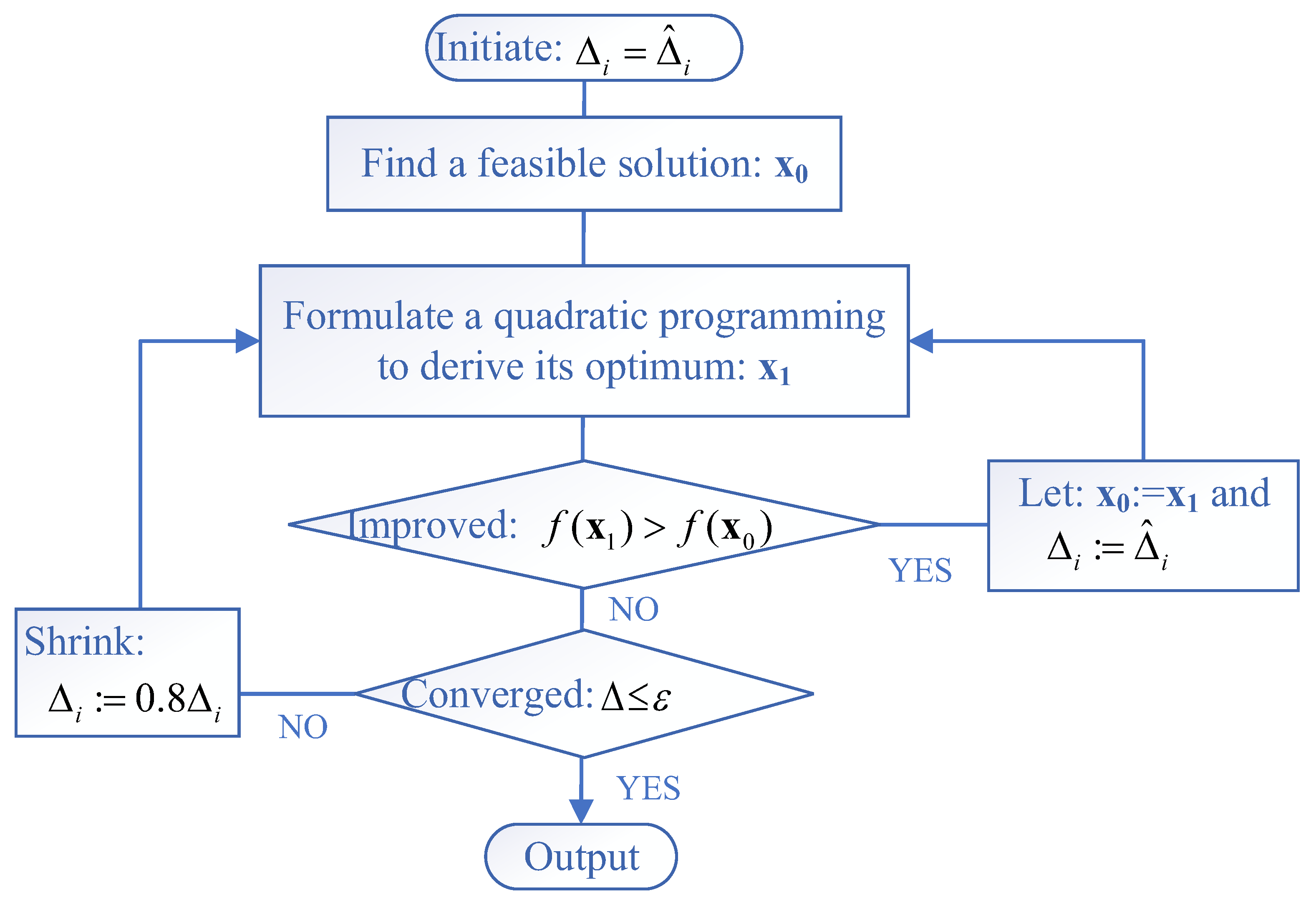
Figure 2 illustrates the flowchart of the solution procedure at a high level. With a trust level (${\Delta }_i$) initiated, the procedure starts with finding a feasible solution (x) to the problem, around which the original problem is approximated with quadratic programming (QP) to derive its optimum (x₁), which, if better than the base solution (x₀) on the original objective, will serve as the base solution, with the trust level restored to its initial one. If the solution has not been improved, then either terminate the procedure if the convergence has been achieved or shrink the trust level by a percentage, for instance, 80%.

3.1. Formulation of a QP Problem

Replacing the water head in (6) and (8) with (9) gives:

$$\begin{array}{l}{P}_{it}=P_i(q_{it},{\overline{V}}_{it},Q_{it})\\ =(A_i{\alpha }_i)\cdot q_{it}{\overline{V}}_{it}-(A_i{\beta }_i)\cdot q_{it}{Q}_{it}+A_i\cdot ({\widehat{Z}}_i^{\mathrm{u}}-{\alpha }_i{\widehat{V}}_i^{(0)}+{\beta }_i{\widehat{Q}}_i^{(0)}-{\widehat{Z}}_i^{\mathrm{d}})\cdot q_{it}\\ =A_i^{(\mathrm{p})}{q}_{it}{\overline{V}}_{it}+B_i^{(\mathrm{p})}{q}_{it}{Q}_{it}+C_i^{(\mathrm{p})}{q}_{it}\end{array}$$

(11)

and

$$\{\begin{array}{l}{q}_{it}\le c_i^{(0)}{h}_{it}+d_i^{(0)}\\ =(c_i^{(0)}{\alpha }_i)\cdot {\overline{V}}_{it}-(c_i^{(0)}{\beta }_i)\cdot Q_{it}+c_i^{(0)}\cdot ({\widehat{Z}}_i^{\mathrm{u}}-{\alpha }_i{\widehat{V}}_i^{(0)}+{\beta }_i{\widehat{Q}}_i^{(0)}-{\widehat{Z}}_i^{\mathrm{d}})+d_i^{(0)}\\ =A_i^{(0)}\cdot {\overline{V}}_{it}+B_i^{(0)}\cdot Q_{it}+C_i^{(0)}\\ q_{it}\le c_i^{(1)}{h}_{it}+d_i^{(1)}\\ =(c_i^{(1)}{\alpha }_i)\cdot {\overline{V}}_{it}-(c_i^{(1)}{\beta }_i)\cdot Q_{it}+c_i^{(1)}\cdot ({\widehat{Z}}_i^{\mathrm{u}}-{\alpha }_i{\widehat{V}}_i^{(0)}+{\beta }_i{\widehat{Q}}_i^{(0)}-{\widehat{Z}}_i^{\mathrm{d}})+d_i^{(1)}\\ =A_i^{(1)}\cdot {\overline{V}}_{it}+B_i^{(1)}\cdot Q_{it}+C_i^{(1)}\end{array}$$

(12)

Substituting (11) for the hydropower output in (1) gives an equivalent objective,

$$\max f(x)={\mathrm{W}}_1\cdot F+{\mathrm{W}}_2\cdot {\displaystyle \sum _{i=1}^N{\displaystyle \sum _{t=0}^{T-1}[A_i^{(\mathrm{p})}{q}_{it}{\overline{V}}_{it}+B_i^{(\mathrm{p})}{q}_{it}{Q}_{it}+C_i^{(\mathrm{p})}{q}_{it}]}}$$

(13)

with x representing the decision variables including: ${\overline{V}}_{it}$, $Q_{it}$, $q_{it}$, etc.

The firm hydropower output (5) will be linearized around the base solution (x₀) that represents the values of decision variables: ${\overline{V}}_{it}^{(0)},Q_{it}^{(0)},q_{it}^{(0)}\mathrm{and}{V}_{it}^{(0)}$, and updated with

$$\begin{array}{l}{\displaystyle \sum _{i=1}^N[A_i^{(\mathrm{p})}{q}_{it}^{(0)}{\overline{V}}_{it}+B_i^{(\mathrm{p})}{q}_{it}^{(0)}{Q}_{it}}\\ +[A_i^{(\mathrm{p})}{\overline{V}}_{it}^{(0)}+B_i^{(\mathrm{p})}{Q}_{it}^{(0)}+C_i^{(\mathrm{p})}](q_{it}-q_{it}^{(0)})+C_i^{(\mathrm{p})}{q}_{it}^{(0)}]\ge F\end{array}$$

(14)

Thus, the QP problem will have a quadratic objective (13) subject to linear constraints: (2)–(4), (10), (12), (14) and a trust corridor,

$$V_{it}^{(0)}-{\Delta }_i\le V_{it}\le V_{it}^{(0)}+{\Delta }_i$$

(15)

where the trust level (${\Delta }_i$) can be initiated as

$${\hat{\Delta }}_i=0.5\left(V_i^{\mathrm{dead}}+\frac{1}{T}{\displaystyle \sum _{t=1}^T{V}_{it}^{\max }}\right)$$

(16)

Solving the QP problem will give its optimum, denoted as x₁ to represent the decision variables: ${\overline{V}}_{it}^{(1)},Q_{it}^{(1)}\mathrm{and}{q}_{it}^{(1)}$, which will determine the original objective with,

$$F^{(1)}=\underset{t}{\min }{\displaystyle \sum _{i=1}^N[A_i^{(\mathrm{p})}{q}_{it}^{(1)}{\overline{V}}_{it}^{(1)}+B_i^{(\mathrm{p})}{q}_{it}^{(1)}{Q}_{it}^{(1)}+C_i^{(\mathrm{p})}{q}_{it}^{(1)}]}$$

(17)

3.2. Finding a Feasible Solution

A feasible solution to the quadratic programming will be determined by solving a problem that

$$\max {\mathrm{W}}_1\cdot Y-{\mathrm{W}}_2\cdot {\displaystyle \sum _{i=1}^N{\displaystyle \sum _{t=1}^{T-1}{\left(V_{it}-V_{it}^{\max }\right)}^2}}$$

(18)

subject to: (2)–(4), (10), (12), (14) and the generating yield (Y),

$${\displaystyle \sum _{i=1}^N{q}_{it}}\ge Y$$

(19)

aimed to approximately maximize the firm hydropower output and the generating efficiency by operating reservoirs at their maximum water levels.

4. Case Studies

4.1. Engineering Background

The models and solution techniques presented in this work are applied to four cascaded hydroplants on the Lower Jinsha River in China, as summarized in

Table 1. Basic parameters of cascaded hydropower reservoirs.

Number	Name	Installed Capacity (MW)	Storage Capacity (GL)	Dam Height (m)	Water Level (m)			Operability
					Flood	Normal	Dead
1	Wudongde	10,200	7408	270	952	975	950	Seasonal
2	Baihetan	16,000	20,600	289	785	825	760	Annual
3	Xiluodu	12,600	12,670	285.5	560	600	540	Annual
4	Xiangjiaba	6400	5163	380	370	380	370	Seasonal

. The Jinsha River has an annual runoff of 4750 m³/s on average, abundant and stable over the years. It is rich in hydropower resources, with a total drop of 3300 m, dropping more than 1 m every kilometer. It flows downstream and contributes to a total exploitable hydropower resource of 100 TW. The lower reaches of the Jinsha River are the most important transportation and regional economic centers in southwest China. Two major storage reservoirs, Baihetan and Xiluodu, have annual operability, making it very important to coordinate the cascaded reservoirs to maximize the benefits of the third-monthly hydropower scheduling.

4.2. Comparison with Dynamic Programming (DP)

The results derived from the SQP will be compared with those produced by the well-known dynamic programming (DP), which, unfortunately, is not favorable for handling multiple reservoirs and therefore applied to only the Wudongde Hydroplant for comparison purposes. Two methods will calculate the water head, hydropower output, and the generating discharge capacity in the same way to ensure a fair and accurate comparison. The DP problem is solved twice: first to maximize the firm power output since it is the top priority, and second to maximize the hydropower production while meeting the firm hydropower output derived the first time, that is, the total hydropower output of all the hydroplants must be no less than the firm hydropower output in each third of a month.

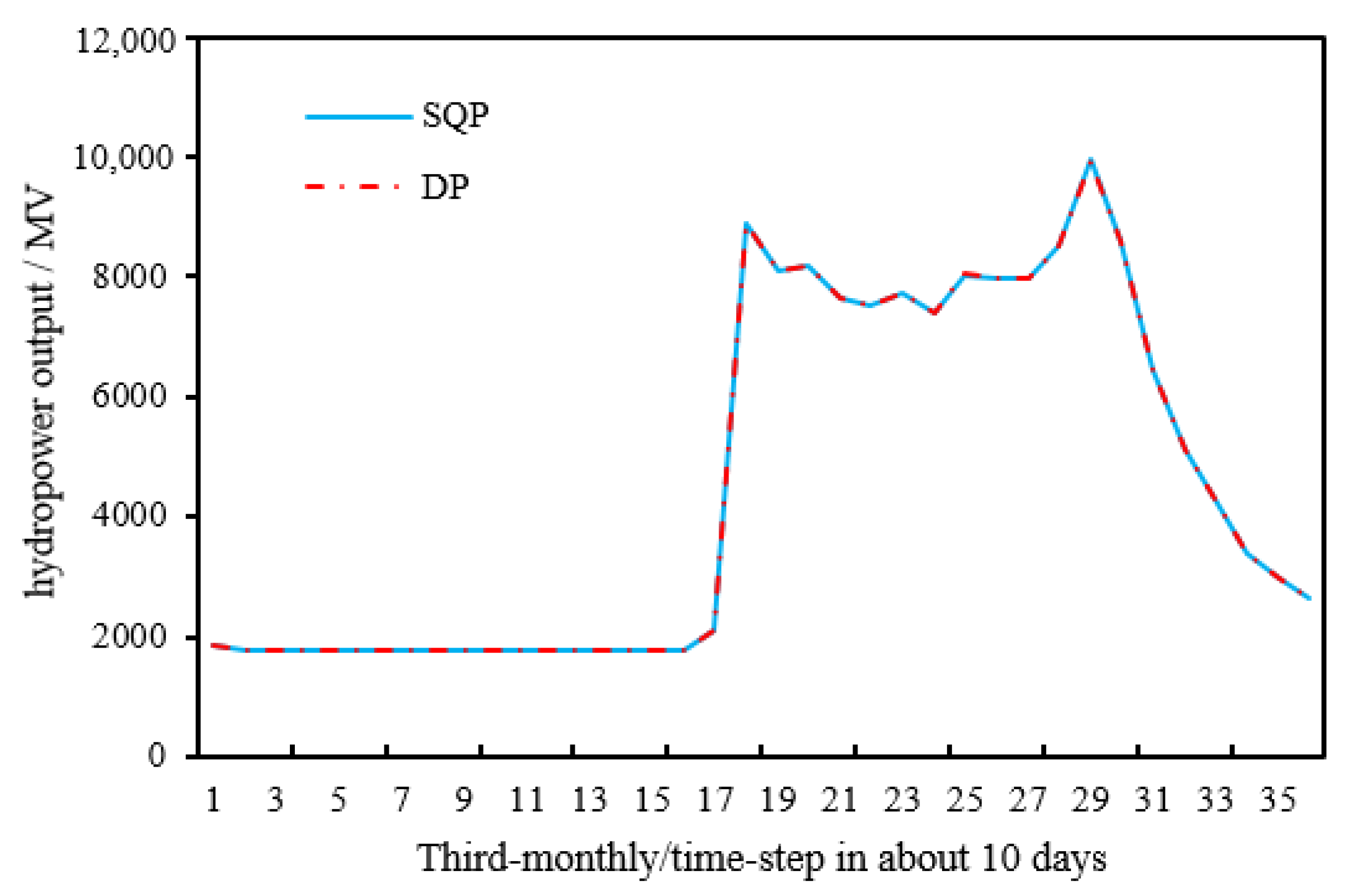
Figure 3 illustrates the results of the third-monthly hydropower outputs derived with the SQP and DP methods, which are very consistent, with only 0.2% at maximum of the difference between the two processes. The hydropower output of Wudongde Hydroplant is flat in dry seasons to maximize the firm hydropower yield and generates more during flood seasons to maximize the annual hydropower production.

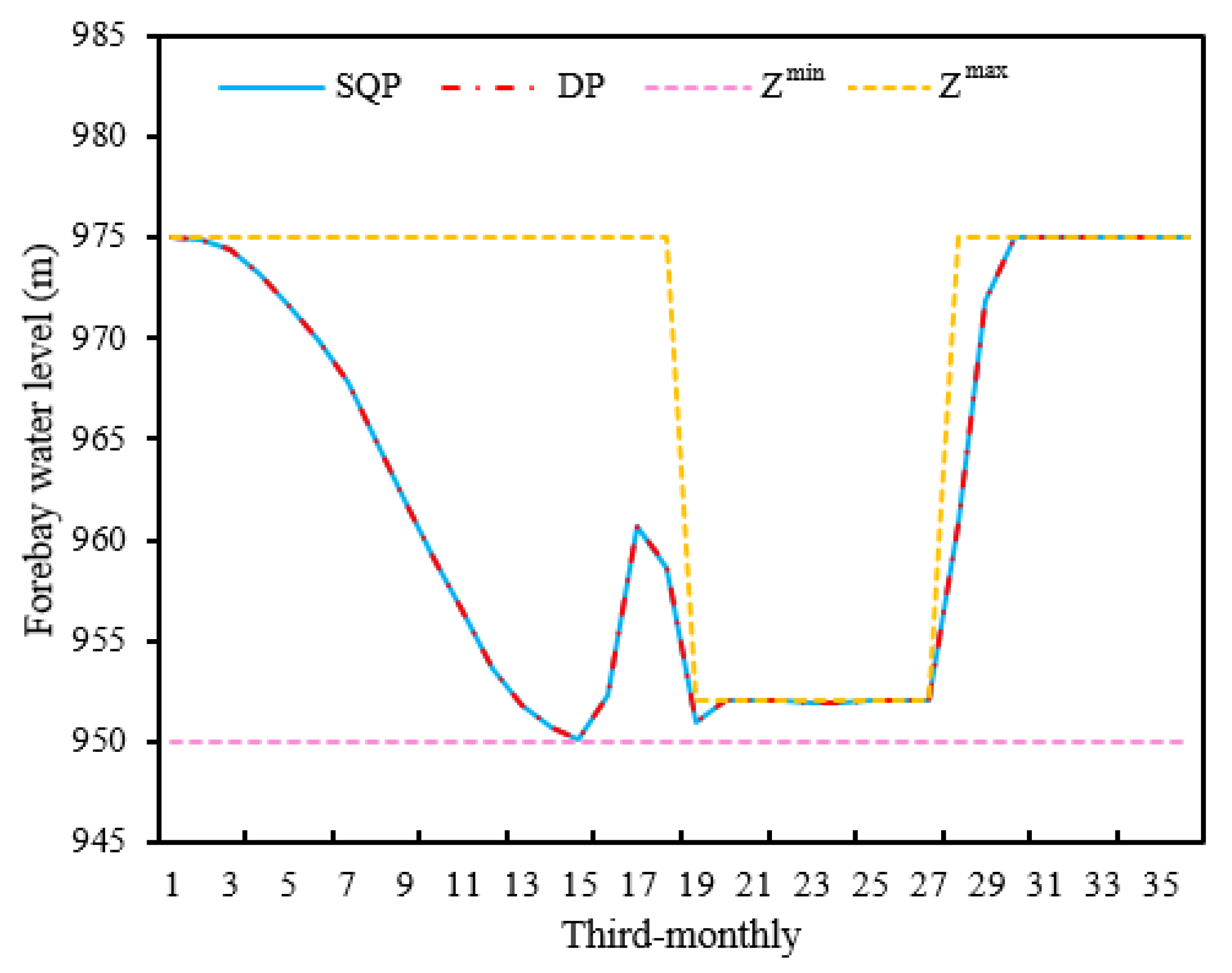
As demonstrated in Figure 4, the third-monthly forebay water levels derived by the DP and SQP for Wudongde Reservoir during the year are also very consistent, with the difference between them within 0.01m. The water level changes within the lower and upper bounds (dotted red lines) and follows a regular pattern: drawing down during dry seasons and then refilling the storage to its full capacity at the end of the flood season. The DP is well known and capable of securing the global optimum for a small-scale problem, and the consistent results suggest that the present SQP is also capable of securing the global optimum.

4.3. Solution Efficiency

The models and procedures are coded in C++ on Microsoft Visual Studio 2019 and run under the Intel Core i5-8250U computer environment, with the Gurobi 9.5.1 as the quadratic programming solver.

Table 2. Algorithm performance index parameters.

Number of Reservoirs	Computing Time(s)	Number of Variables		Number of Constraints
		Model 1	Model 2	Model 1	Model 2
4	61.784	725	725	1348	1644
3	46.478	544	544	1020	1242
2	17.981	363	363	1242	840
1	7.444	182	182	364	438

summarizes the problem scales and the solution efficiency in four case studies, with one, two, three, and four reservoirs included. Each case study involves two models to be solved: Model 1 to derive an initial solution, and Model 2 to be a quadratic programming problem that is successively solved. The two models have the same number of variables, but Model 2, with the trust corridor constraints included, has more constraints than Model 1. The results show that the computational time increases somewhat linearly as the number of reservoirs increases, and it takes about 1 min to solve the problem involving all four cascaded hydropower reservoirs, while the DP takes about 4 min to secure the optimum to the problem involving only one reservoir.

4.4. Convergence of the Method

Figure 5 illustrates the converging process of the objective function value, which is monotonically increasing and ensured a fast convergence to a limit, with the second iteration contributing to the most significant improvement by about 20% while the following iterations improved by only about 1%, and the convergence is achieved at the fourth or fifth iteration.

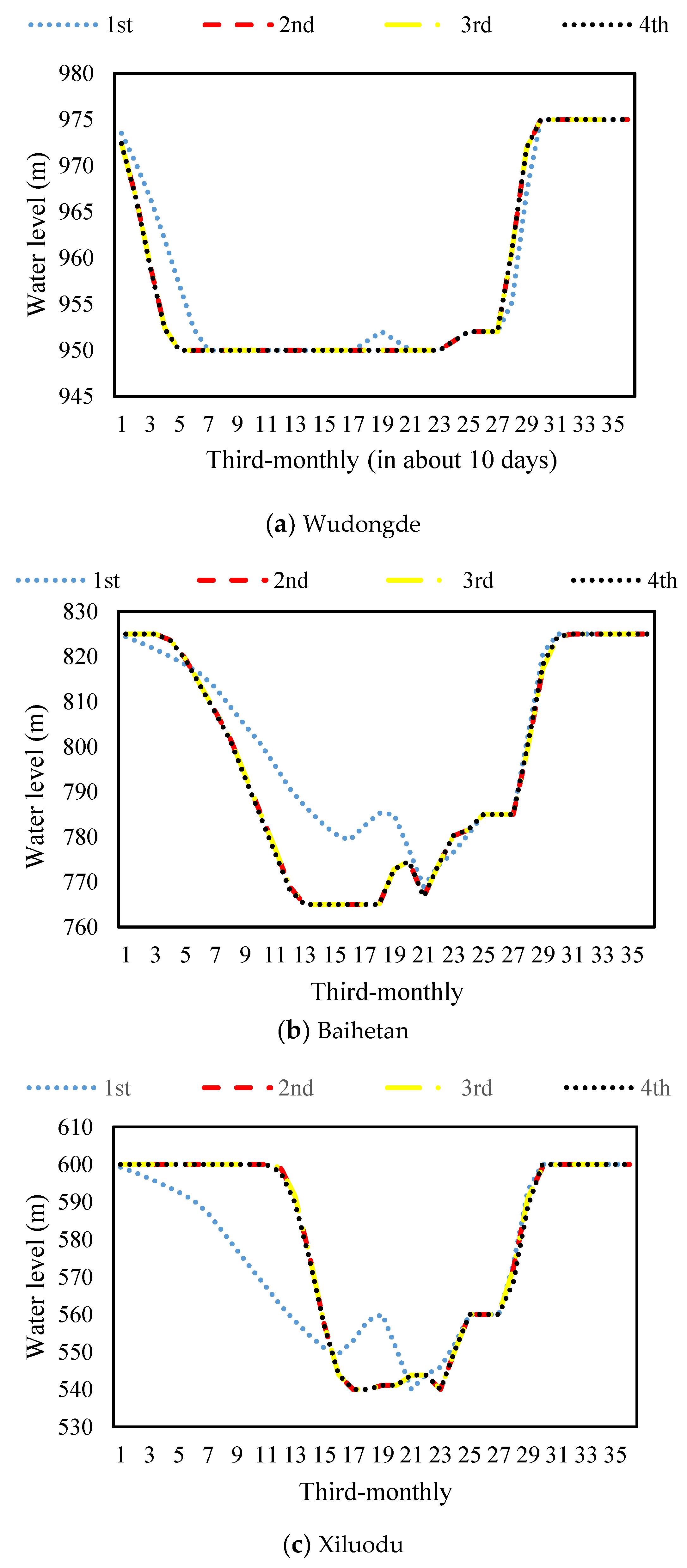
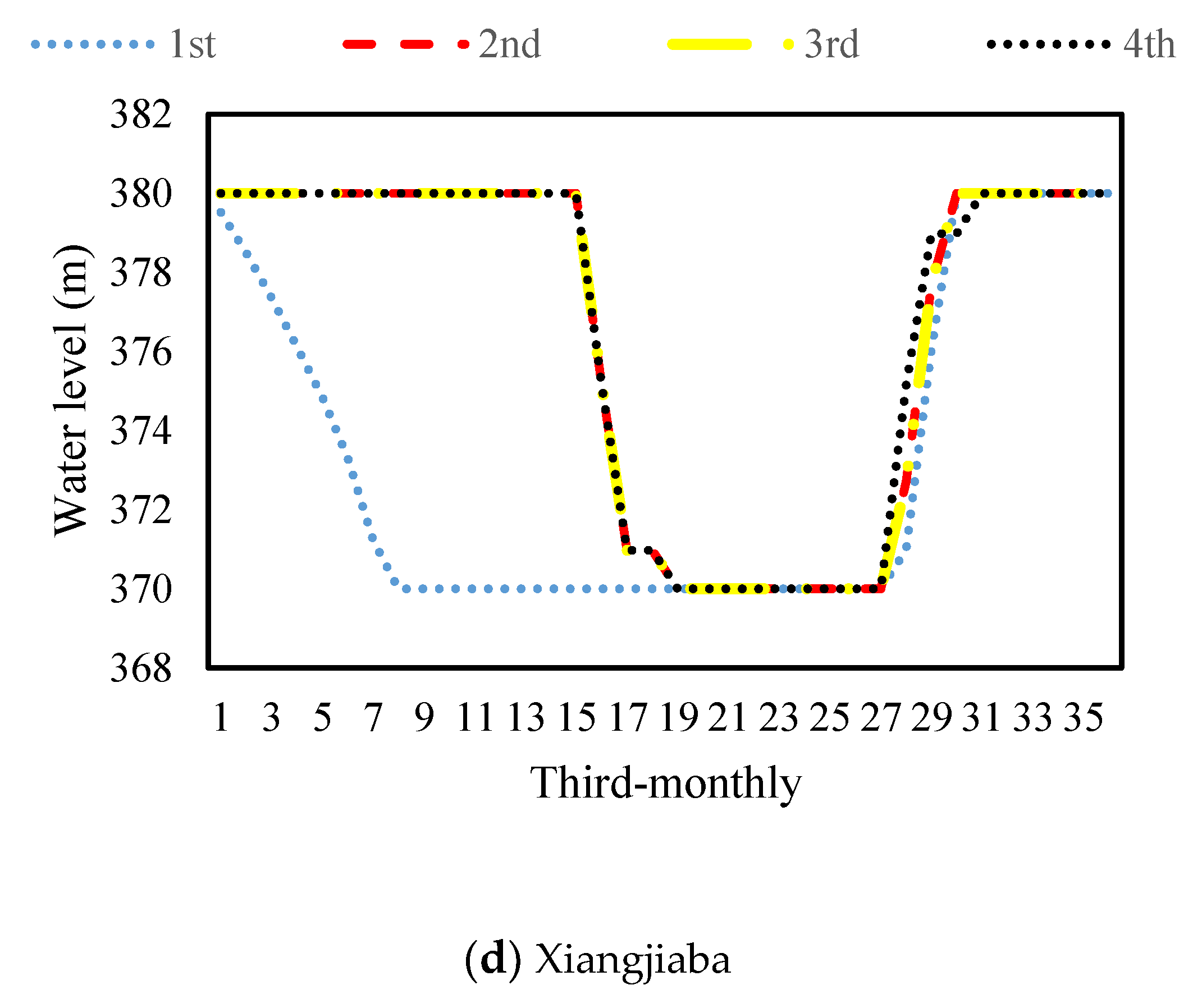
Figure 6 shows the convergence process of water levels in the first four iterations. For all four reservoirs, the third-monthly water levels converge to be in a narrow corridor after only one iteration, suggesting a very fast convergence of the procedure.

4.5. Results in Detail

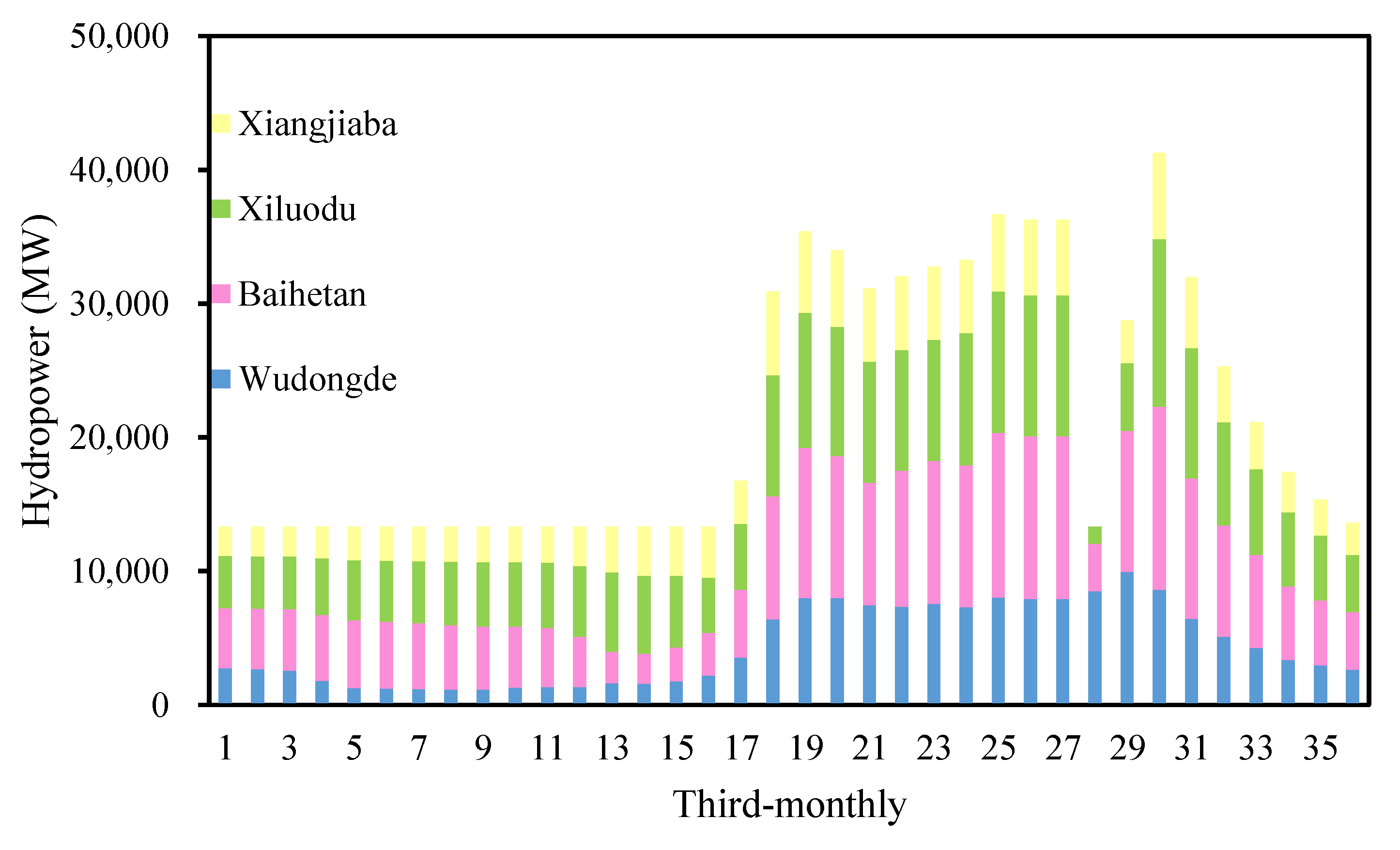
Figure 7 shows the third-monthly hydropower outputs scheduled over a year for cascaded individual hydroplants on the Jinsha River. The cascaded hydropower reservoirs coordinate very well to maximize the firm hydropower output at the top priority by regulating their storage capacities to give a constant power yield during the dry seasons, and then make full use of their installed capacities to convert the coming inflows into hydropower energy as much as possible during the flood seasons.

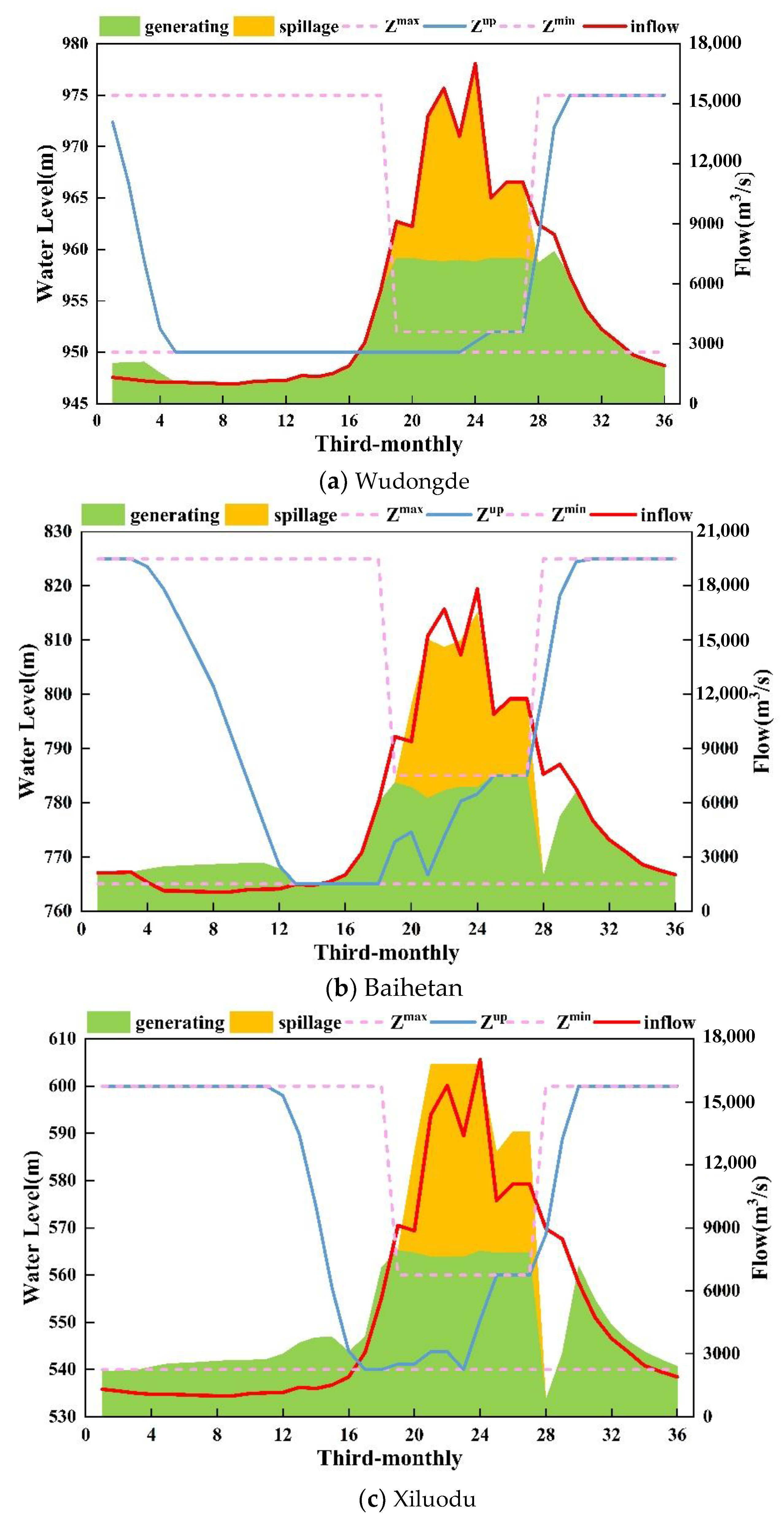
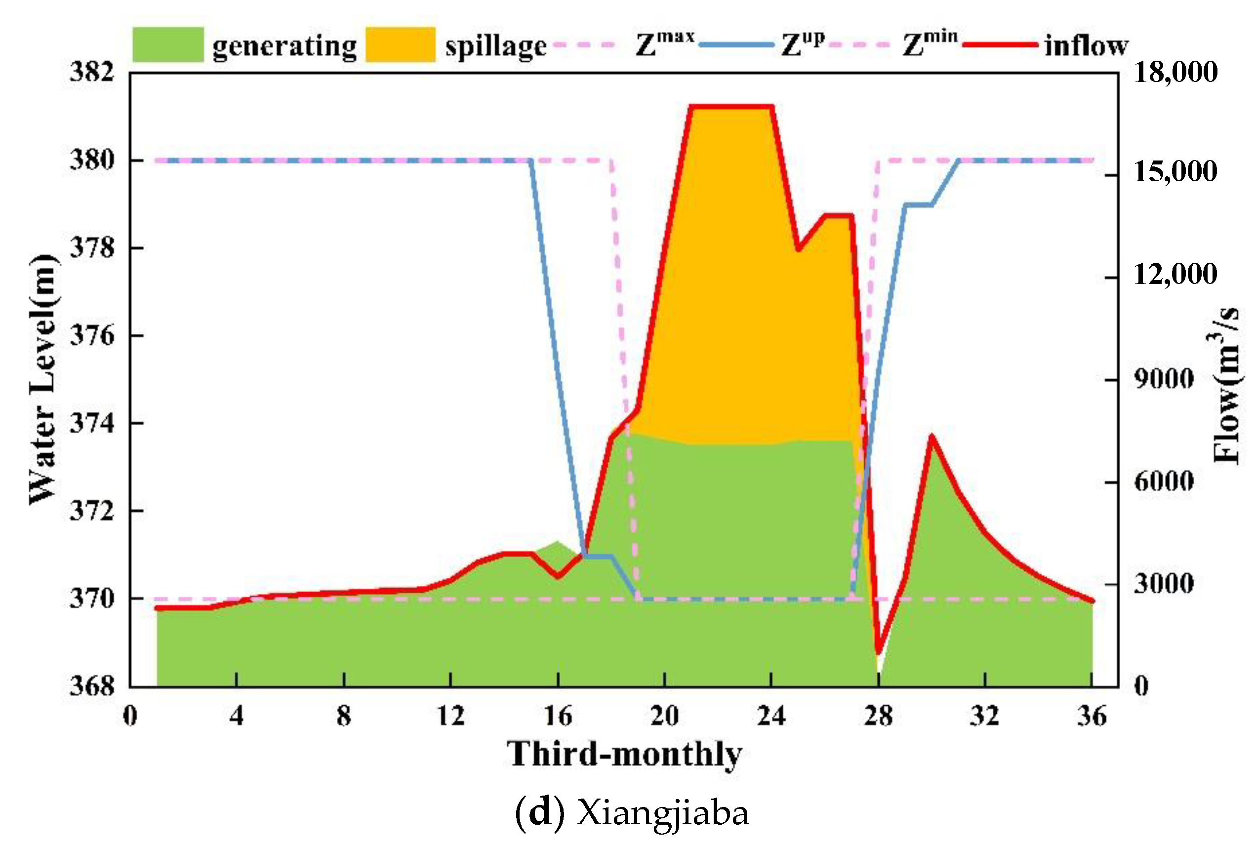
Figure 8 illustrates the optimal scheduling process of the four cascaded hydropower reservoirs. The cumulative area of the generating discharge (marked green) and the spillage (marked orange) represents the outflow from the reservoir. As indicated by the water balance, a reservoir draws down its storage when the outflow is greater than the inflow, or keeps it unchanged when they are the same, or refills its storage capacity when the inflow is larger than the outflow. Each reservoir regulates its water level between the lower bound, which is enforced at the dead level, and the upper bound, which is enforced at its normal level during dry seasons, and at its flood-control level during flood seasons, following a reasonable pattern of emptying its storage capacity during dry seasons and then refilling it during flood seasons. The Baihetan and Xiluodu demonstrate greater flexibility in regulating their storages, which change more smoothly to their full extent over the year. The plentiful runoffs during flood seasons incur spillages in large amounts, which cannot be avoided since the hydroplants have fully used their storage and installed capacities.

5. Conclusions

This work formulates a third-monthly hydropower scheduling model into a quadratic programming (QP) problem, which incorporates nonlinear functions, including the generating discharge capacity that is linearly concaved with two planes defined as functions of storage and release of a reservoir, the total firm hydropower output that is approximated with the first-order expansion and successively updated before solving the QP problem, along with the hydropower output that is expressed as a quadratic function of three variables: the storage, the release, and the generating discharge.

The models and procedures are applied to four cascaded hydropower reservoirs on the Jinsha River, with the results suggesting:

(1)

Successive quadratic programming (SQP) can derive results consistent with dynamic programming (DP), which is well known and capable of securing the global optimal solution to a small-scale problem.

(2)

The present procedure has the computational time increasing linearly as the number of reservoirs increases, taking about 1 min to solve the problem involving all four cascaded hydropower reservoirs.

(3)

The convergence of the SQP can be achieved at the fifth iteration, with objective functional value monotonically increasing and improving the most significantly in the second iteration by about 20%, while in the following iterations by only about 1%.

(4)

The cascaded hydropower reservoirs coordinate very well to maximize the firm hydropower output at the top priority by regulating their storage capacities to give a constant power yield during the dry seasons, and then making full use of their installed capacities to convert the coming inflows into hydropower energy as much as possible during the flood seasons.

It is worth noting that the present model only presents a simplified real-world problem, based on which the present solution procedure is verified to ensure consistent results with the DP formulation that may have strength over the present modeling in approaching a real-world problem.

Under a deterministic optimization framework, the present model and procedure are more recommended in preliminary assessment with historical inflows observed than in a year-ahead hydropower scheduling, since the monthly inflows in a coming year are often too uncertain to be accurately forecasted. However, it is possible that the modeling techniques and procedure in this work can be extended to an hourly hydropower scheduling problem, since the hourly inflows can now be forecasted at very high accuracy.

References

- Allen, R.B.; Bridgeman, S.G. Dynamic Programming in Hydropower Scheduling. J. Water Resour. Plan. Manag. 1986, 112, 339–353. [Google Scholar] [CrossRef]
- Wang, C.; Zhou, J.; Lu, P.; Yuan, L. Long-term scheduling of large cascade hydropower stations in Jinsha River, China. Energy Convers. Manag. 2015, 90, 476–487. [Google Scholar] [CrossRef]
- Yang, Z.; Liu, P.; Cheng, L.; Wang, H.; Ming, B.; Gong, W. Deriving operating rules for a large-scale hydro-photovoltaic power system using implicit stochastic optimization. J. Clean. Prod. 2018, 195, 562–572. [Google Scholar] [CrossRef]
- Zambelli, M.S.; Soares, S.; Silva, D.D. Deterministic versus stochastic dynamic programming for long term hydropower scheduling. In Proceedings of the 2011 IEEE Trondheim PowerTech, Trondheim, Norway, 19–23 June 2011; pp. 1–7. [Google Scholar]
- Martins, L.S.A.; Azevedo, A.T.; Soares, S. Nonlinear Medium-Term Hydro-Thermal Scheduling With Transmission Constraints. IEEE Trans. Power Syst. 2014, 29, 1623–1633. [Google Scholar] [CrossRef]
- Zheng, H.; Feng, S.; Chen, C.; Wang, J. A new three-triangle based method to linearly concave hydropower output in long-term reservoir operation. Energy 2022, 250, 123784. [Google Scholar] [CrossRef]
- Yakowitz, S. Dynamic programming applications in water resources. Water Resour. Res. 1982, 18, 673–696. [Google Scholar] [CrossRef]
- Heidari, M.; Chow, V.T.; Kokotović, P.V.; Meredith, D.D. Discrete Differential Dynamic Programing Approach to Water Resources Systems Optimization. Water Resour. Res. 1971, 7, 273–282. [Google Scholar] [CrossRef]
- Li, C.; Zhou, J.; Ouyang, S.; Ding, X.; Chen, L. Improved decomposition–coordination and discrete differential dynamic programming for optimization of large-scale hydropower system. Energy Convers. Manag. 2014, 84, 363–373. [Google Scholar] [CrossRef]
- Turgeon, A. Optimal short-term hydro scheduling from the principle of progressive optimality. Water Resour. Res. 1981, 17, 481–486. [Google Scholar] [CrossRef]
- Cheng, C.; Shen, J.; Wu, X.; Chau, K.-w. Short-Term Hydroscheduling with Discrepant Objectives Using Multi-Step Progressive Optimality Algorithm1: Short-Term Hydroscheduling with Discrepant Objectives Using Multi-step Progressive Optimality Algorithm. J. Am. Water Resour. Assoc. 2012, 48, 464–479. [Google Scholar] [CrossRef]
- Zhou, Y.; Guo, S.; Chang, F.-J.; Xu, C.-Y. Boosting hydropower output of mega cascade reservoirs using an evolutionary algorithm with successive approximation. Appl. Energy 2018, 228, 1726–1739. [Google Scholar] [CrossRef]
- Ahmed, J.A.; Sarma, A.K. Genetic Algorithm for Optimal Operating Policy of a Multipurpose Reservoir. Water Resour. Manag. 2005, 19, 145–161. [Google Scholar] [CrossRef]
- Jothiprakash, V.; Arunkumar, R. Optimization of Hydropower Reservoir Using Evolutionary Algorithms Coupled with Chaos. Water Resour. Manag. 2013, 27, 1963–1979. [Google Scholar] [CrossRef]
- Chang, Y.T.; Chang, L.C.; Chang, F.J. Intelligent control for modeling of real-time reservoir operation, part II: Artificial neural network with operating rule curves. Hydrol. Process. 2005, 19, 1431–1444. [Google Scholar] [CrossRef]
- Chaves, P.; Chang, F.J. Intelligent reservoir operation system based on evolving artificial neural networks. Adv. Water Resour. 2008, 31, 926–936. [Google Scholar] [CrossRef]
- Reddy, M.J.; Nagesh Kumar, D. Multi-objective particle swarm optimization for generating optimal trade-offs in reservoir operation. Hydrol. Process. 2007, 21, 2897–2909. [Google Scholar] [CrossRef]
- Zhang, X.; Yu, X.; Qin, H. Optimal operation of multi-reservoir hydropower systems using enhanced comprehensive learning particle swarm optimization. J. Hydro-Environ. Res. 2016, 10, 50–63. [Google Scholar] [CrossRef]
- Bai, T.; Kan, Y.B.; Chang, J.X.; Huang, Q.; Chang, F.J. Fusing feasible search space into PSO for multi-objective cascade reservoir optimization. Appl. Soft. Comput. 2017, 51, 328–340. [Google Scholar] [CrossRef]
- Needham, J.T.; Watkins, D.W.; Lund, J.R.; Nanda, S.K. Linear Programming for Flood Control in the Iowa and Des Moines Rivers. J. Water Resour. Plan. Manag. 2000, 126, 118–127. [Google Scholar] [CrossRef]
- Consoli, S.; Matarazzo, B.; Pappalardo, N. Operating rules of an irrigation purposes reservoir using multi-objective optimization. Water Resour. Manag. 2008, 22, 551–564. [Google Scholar] [CrossRef]
- Feng, Z.-K.; Niu, W.-J.; Jiang, Z.-Q.; Qin, H.; Song, Z.-G. Monthly Operation Optimization of Cascade Hydropower Reservoirs with Dynamic Programming and Latin Hypercube Sampling for Dimensionality Reduction. Water Resour. Manag. 2020, 34, 2029–2041. [Google Scholar] [CrossRef]
- Zhang, Y.; Jiang, Z.; Ji, C.; Sun, P. Contrastive analysis of three parallel modes in multi-dimensional dynamic programming and its application in cascade reservoirs operation. J. Hydrol. 2015, 529, 22–34. [Google Scholar] [CrossRef]
- Yoo, J.-H. Maximization of hydropower generation through the application of a linear programming model. J. Hydrol. 2009, 376, 182–187. [Google Scholar] [CrossRef]
- dos Santos Abreu, D.L.; Finardi, E.C. Continuous Piecewise Linear Approximation of Plant-Based Hydro Production Function for Generation Scheduling Problems. Energies 2022, 15, 1699. [Google Scholar] [CrossRef]
- Vielma, J.P. Mixed Integer Linear Programming Formulation Techniques. SIAM Rev. 2015, 57, 3–57. [Google Scholar] [CrossRef]
- Azevedo, A.T.; Oliveira, A.R.L.; Soares, S. Interior point method for long-term generation scheduling of large-scale hydrothermal systems. Ann. Oper. Res. 2008, 169, 55. [Google Scholar] [CrossRef]
- Zhou, B.; Feng, S.; Xu, Z.; Jiang, Y.; Wang, Y.; Chen, K.; Wang, J. A Monthly Hydropower Scheduling Model of Cascaded Reservoirs with the Zoutendijk Method. Water 2022, 14, 3978. [Google Scholar] [CrossRef]
- Shang, Y.; Lu, S.; Gong, J.; Liu, R.; Li, X.; Fan, Q. Improved genetic algorithm for economic load dispatch in hydropower plants and comprehensive performance comparison with dynamic programming method. J. Hydrol. 2017, 554, 306–316. [Google Scholar] [CrossRef]
- Zheng, J.; Yang, K.; Lu, X. Limited adaptive genetic algorithm for inner-plant economical operation of hydropower station. Hydrol. Res. 2013, 44, 583–599. [Google Scholar] [CrossRef]
- Grygier, J.C.; Stedinger, J.R. Algorithms for optimizing hydropower system operation. Water Resour. Res. 1985, 21, 1–10. [Google Scholar] [CrossRef]
- Cheng, X.; Feng, S.; Zheng, H.; Wang, J.; Liu, S. A hierarchical model in short-term hydro scheduling with unit commitment and head-dependency. Energy 2022, 251, 123908. [Google Scholar] [CrossRef]
- Catalão, J.P.S.; Pousinho, H.M.I.; Mendes, V.M.F. Scheduling of head-dependent cascaded hydro systems: Mixed-integer quadratic programming approach. Energy Convers. Manag. 2010, 51, 524–530. [Google Scholar] [CrossRef]
- Niu, W.-J.; Feng, Z.-K.; Cheng, C.-T. Optimization of variable-head hydropower system operation considering power shortage aspect with quadratic programming and successive approximation. Energy 2018, 143, 1020–1028. [Google Scholar] [CrossRef]
- Díaz, G.E.; Fontane, D.G. Hydropower Optimization Via Sequential Quadratic Programming. J. Water Resour. Plan. Manag. 1989, 115, 715–734. [Google Scholar] [CrossRef]
- Arnold, E.; Tatjewski, P.; Wołochowicz, P. Two methods for large-scale nonlinear optimization and their comparison on a case study of hydropower optimization. J. Optim. Theory Appl. 1994, 81, 221–248. [Google Scholar] [CrossRef]
Figure 1.
Capacity of generating discharge due to water head.
Figure 2.
Flowchart of the solution procedure.
Figure 3.
Third-monthly hydropower outputs from two methods.
Figure 4.
Third-monthly water levels derived with two methods.
Figure 5.
The converging process of the objective function value.
Figure 6.
The convergence of water levels of the reservoirs.
Figure 7.
Third-monthly hydropower schedules in a year.
Figure 8.
Results of third-monthly water levels and flows over a year.