
Spatial Variations of Fabric and Microstructure of Blue Ice Cores at the Shear Margin of Dalk Glacier, Antarctica
by
 , , and
Siyu Lu
1,2,
Nan Zhang
1,*,
Danhe Wang
3,
Guitao Shi
3,
Tianming Ma
4,
Hongmei Ma
2,
Chunlei An
2 and
Yuansheng Li
1,2,* 1
Polar Research Center, Institute for Polar Science and Engineering, College of Construction Engineering, Jilin University, Changchun 130021, China
2
Polar Research Institute of China, Shanghai 200136, China
3
Key Laboratory of Geographic Information Science, School of Geographic Sciences, East China Normal University, Shanghai 200241, China
4
School of Earth and Space Sciences, University of Science and Technology of China, Hefei 230026, China
*
Authors to whom correspondence should be addressed.
Water 2023, 15(4), 728; https://doi.org/10.3390/w15040728
Submission received: 23 January 2023
/
Revised: 8 February 2023
/
Accepted: 9 February 2023
/
Published: 12 February 2023
(This article belongs to the Special Issue Sea, River, Lake Ice Properties and Their Applications in Practices)
Abstract
:The study of the fabric and microstructure of ice at the shear margin of the Antarctic ice sheet is of great significance for understanding the ice flow and its contributions to sea level rise. In this study, twenty-three one-meter-long ice cores were drilled from blue ice areas at the shear margin of the Dalk Glacier, Antarctica. The ice fabric and microstructure of these ice cores are analyzed using a G50 fabric analyzer. This study shows that the shallow ice cores in this region present a cluster fabric as a consequence of shear stress. The grain size decreases following the direction of the ice flow towards the exposed bedrock at the end of the glacier, due to the blocking and squeezing by the bedrock. The formation mechanism of the shallow ice layers is that the ice from the original accumulation area flows here, lifted by the bedrock and shaped by the summer ablation and denudation. The basal ice at the shear margin of the Dalk Glacier is strongly rubbed by the bedrock and demonstrates a cluster fabric. The analysis of stable water isotopes shows a weak negative correlation between shallow ice fabric and stable water isotopes with depth. Bedrock topography and shear stress have a greater influence on grain microstructure among different ice cores over long distances at shear margins.
1. Introduction
The Antarctic and Greenland ice sheets are the most important contributors to sea level rise this century as a result of global warming [1,2,3]. The Antarctic ice sheet is formed by the accumulation of snow, which is transformed into firn and ice by a process called densification. After this process, ice is anisotropic under the initial natural conditions. During the process of ice sheet flow, large-scale anisotropy is formed in the ice, which is called fabric (also described in the literature as ‘Crystallographic Preferred Orientation’, ‘lattice preferred orientation’, or ‘texture’) [4,5,6,7]. Ice sheet flow comprises internal deformation and external deformation, which is mainly the basal slip caused by gravity and tidal forces [5,8,9]. Antarctic ice flow velocity is slow at the dome and fast at the shear margin. The shear margin also accelerates the melting of the ice shelf [10]. The fabric and microstructure of natural ice change under the influence of deformation during its movement from the dome to the margin of the ice sheet. This process comprises the formation and evolution of fabric, changes in grain size, and the dynamic recrystallization of microstructures [5,11,12,13,14].
Currently, researches on the ice fabric of Antarctic ice cores mainly focus on deep ice cores, such as the Vostok deep ice core, Dome C deep ice core, EDML deep ice core, and Dome Fuji deep ice core [15,16,17,18,19]. An ice sheet moves more slowly at domes and ice divides, where ice cores are less affected by ice flow. The flow of ice streams strongly affects the stability of the polar ice sheet [5,20,21,22]. The basal and lateral shear margins are the key regions that affect the dynamics of glacier flow [23,24]. The subglacial bedrock and the shear margin bedrock create drag forces at the interface with the glacier that impede the movement of the ice flow, which has a strong influence on an ice flow and mass transport. Especially in blue ice areas near the margin of the ice sheet, where the thickness of the ice sheet is rapidly getting thinner, the bedrock has a greater effect on the microstructure of the ice. In addition to the evolution of ice fabric, the bubbles trapped in ice also undergo significant changes such as elongation, shearing, and fragmentation during the glacial movement. The microscopic morphology and evolution of bubbles can be affected by the ice grains, and in turn, impact the development of ice grains.
In laboratory experiments, the deformation process of pure polycrystalline ice under shear forces simulates the fabric and microstructure of ice flow in the ice sheet margin region [25,26,27,28,29]. Under natural conditions, the ice fabric development in the ice sheet margin region is affected by temperature, impurity content, and structural heterogeneity, with depth and spatial variations [30,31,32,33]. To date, few studies have directly studied fabric from temperate and polar glacier margin regions [11,34,35,36,37,38,39]. In geophysical studies, ice radar-sounding techniques are used to detect large-scale ice fabric in glaciers [22,40,41,42,43,44,45,46,47]. For mountain glaciers, a study on fabric and microstructures of ice could provide a micro perspective for understanding the ice flow and predicting related disasters such as ice avalanches [48]. Solar radiative transfer [49], synthetic aperture radar, and optical satellite monitoring [50,51,52] are also sensitive to ice microstructures at different scales.
In this study, by using the G50 fabric analyzer [53], we analyzed the ice fabric and microstructure of twenty-tree one-meter-long ice cores drilled from the shear margin of the Dalk Glacier, Antarctica. In addition, the stable water isotopes were analyzed by a Picarro L-2130i Water Isotope Analyzer. The depth and spatial variations of the fabrics, microstructures, and stable water isotopes of ice cores in this shear margin were studied. Then, the formation mechanism and the influence of the subglacial bedrock on the ice were discussed. The results of this study can be used as a reference for comparisons between field study and laboratory experiments and improving the ice flow models at the shear margins of the ice sheet.
2. Materials and Methods
2.1. Sample Collection
The twenty-three 1 m-long shallow ice cores used in this study were drilled during 2019–2020 field season of 36th Chinese National Antarctic Research Expedition. The sampling site, as shown in Figure 1, was selected from the fast-flow area at the margin of the Dalk Glacier, East Antarctic. As seen in Figure 1, the ice flows in the direction from inland toward the coast. Drill sites IC, IW, and OIW were selected based on the ice flow direction. Ice cores numbered IC1 to IC7 were drilled in the direction of ice flow, from far to near the exposed subglacial bedrock. Ice cores labeled IC were drilled vertically downward from the glacier surface to a depth of 1 m. The IW and OIW ice cores were drilled from the basal regions of the ice flow at two different locations, in a horizontal direction, drilled into the ice ‘wall’. The IW ice cores consisted of five separate cores in the front of an exposed bedrock. IW1 to IW3 are three cores from bottom to top at the same location, with adjacent cores spaced 20 cm apart, while IW4 to IW6 are three cores from bottom to top at another location, with adjacent cores spaced 20 cm apart. IW7 was a separate core from a third location. Nine OIW ice cores were taken from another three locations in a similar way, as shown in Figure 1. Detailed information about the basic information of the drill sites is shown in Table 1.
All ice cores were drilled using a portable hand-held gasoline drill. After the ice cores were drilled, basic information was measured and recorded in the field. Afterward, the ice cores were put into insulated foam boxes and shipped back to the Ice Laboratory of the Polar Research Institute of China in a low-temperature container; throughout this process, the temperature of the ice was maintained at −20 °C. Unfortunately, we did not mark the relative direction between the cores and the ice flow when the ice cores were recovered in the field. It was no longer possible to determine the orientation information of the ice cores relative to the direction of ice flow. Furthermore, there were occasional breaks in the drilling process of each core, and the relative rotation angles of the upper and lower ice cores could not be identified since no mark was made at these breaks.
2.2. Thin Sections Preparation and Fabric Analysis
In the low-temperature laboratory at −20 °C, the ice cores were cut and subsampled using a band saw. The ice core samples were cut 1 cm thick and then made into thin sections by the microtome. The thin sections were glued to glass plates by dropping ultrapure water at four corners or all around them. Thin sections of IC ice cores were continuously made for the whole 1 m-long ice cores, and the direction was vertical to the surface (parallel to the drilling direction). For IW and OIW ice cores, only one sample was taken from each core for thin sections preparation since the rest of the cores were used for analysis of other proxies, such as gas analysis. Both horizontal and vertical thin sections were made for IW7 and OIW6.
The length of the thin sections ranges from 3 to 10 cm depending on the actual conditions of the ice samples. The thickness of thin sections was 200–400 μm. A total of 98 thin sections were made for all 23 ice cores for ice fabric and microstructure studies. Afterward, the thin sections were scanned and analyzed using a G50 ice fabric analyzer to obtain image data such as c-axes orientation maps and microstructure maps of the ice.
2.3. Stable Water Isotope Analysis
Stable water isotope analysis of the IC ice cores was performed by continuous sampling of the whole ice cores. IW and OIW ice cores took only 1 sample per core for isotope analysis. Ice samples for stable water isotope analysis were prepared during the process of making thin sections. Each of the samples were approximately 5–10 g. Then, the samples were melted in the ultra-clean laboratory. A total of 2 mL of the melted water samples were taken into clean sampling bottles and analyzed using Picarro L-2130i Water Isotope Analyzer.
We used 1 set of standard samples for quality control. Six secondary standard samples were prepared by mixing V-SMOW (absolute ratio 18O/16O = (2005.20 ± 0.43) × 10−6, relative ratios δ18O = 0‰ and δD = 0‰) and V-SLAP (δ18O = −55.50‰ and δD = −428‰) in different ratios, and three of them with corresponding δ18O were at −14.22‰, −19.88‰ and −27.53‰, respectively, and the corresponding δD was at −104.71‰, −148.62‰ and −208.63‰.
2.4. Image Data Processing Methods
The images obtained by the G50 fabric analyzer were used for grain and bubble microstructure analysis using MorphoLibJ [54], a deep learning plugin in Fiji Image J [55] software, and Trainable Weka Segmentation [56], a machine learning plugin in Fiji Image J software. To reduce noises, bubbles with area less than 0.1 mm2 were removed. Incomplete small ice grains at the cutting edges of thin sections were removed when calculating grain sizes. The results of the grain and bubble analysis were also checked with the manually counted number of grains and bubbles.
3. Results
A total of 98 thin section samples were analyzed in this study. In this section, the results of six representative ice cores are presented in detailed figures. For IC1 and IC3 samples, the topmost and bottommost two samples of ice cores were selected, and IW5 and OIW5 ice cores were selected from horizontally drilled ice cores at the basal regions. In total, ten thin sections were chosen as typical samples, as shown from Figure 2, Figure 3, Figure 4, Figure 5 and Figure 6. Data from all other samples were also analyzed and presented in other figures and curves in this paper.
3.1. Microstructures of Ice Thin Sections
The microstructure maps of the selected 10 typical thin sections are shown in Figure 2. As shown in the figure, the surrounding ice band is frozen pure water, which is used to fix the thin section. The areas that show different colors are ice grains. The transparent parts surrounded by ice grains are bubbles.
3.2. Ice Fabrics
The fabric data were analyzed using a G50 Fabric Investigator. The c-axis orientation of each grain was determined by manually selecting each ice grain, and the c-axis orientation histograms are shown in Figure 3a. The c-axis orientation data were plotted in polar coordinates to obtain the kernel contour maps, as shown in Figure 3b. Figure 3c shows the microstructure maps with colored orientations of each grain. Normally, when analyzing the fabric of deep ice cores, samples will be selected at an interval of dozens of meters. In this study, the IC1–IC7 ice cores were sampled continuously for fabric analysis. According to the kernel contour maps of the ice fabric, ice is mainly presented as a cluster fabric, and the clusters are usually 0° and 180°. However, the samples in different layers show some angular shift of cluster orientation.
3.3. Microstructure of Grains
Figure 4a shows the grain size frequency distributions. Grain circularity frequency distributions are presented in Figure 4b. Grain ellipse elongation frequency distributions are presented in Figure 4c. Circularity = 4π(A/P2), where A = area, P = perimeter, and 1.0 is a perfect circle.
As shown in Figure 4a, the grain size distributions are skewed, with the majority of grains plotting toward finer grain sizes and a tail extending toward larger grain sizes. As shown in Figure 4c, grain ellipse elongation (dlong axis/dshort axis) plots are skewed toward lower values, with some ratios extending toward values > 3. The averages of the grain axial ratio in these samples range from 1.5 to 1.8.
3.4. Microstructure of Bubbles
In general, the large-area scanning macroscope (LASM) method is used to analyze the properties of bubbles trapped in ice cores. In this study, the bubble characteristics were analyzed by analyzing microscopic images of ice thin sections scanned by a G50 fabric analyzer.
Bubble diameter frequency diagrams are skewed toward smaller bubble sizes. Most bubbles have diameters <1 mm, except the very shallow ice samples of IC ice cores (Figure 5a). Bubble circularity frequency diagrams are skewed to 1, with a small percentage of bubbles <0.5 (Figure 5b). The axial ratio (dlong axis/dshort axis) of bubbles distributes on a large scale, which means the bubbles have a more elongated shape characteristic.
3.5. Shape-Preferred Orientations (SPOs) of Ice Grains and Bubbles
Shape-preferred orientations (SPOs) are defined as the major axis orientation of each grain. In this study, the direction of the maximum Feret diameter is used to represent the shape preference orientations. The diameter passing through the center of a grain in any direction is called a Feret diameter. As shown in Figure 6, the angles of the maximum Feret diameters of ice grains and bubbles in the selected ten representative thin sections are plotted in the rose diagrams. Samples such as IW5 and OIW5 have a relatively strong grain SPO at angles around 20° anti-clockwise of the c-axis maximums. The SPOs of IC ice cores are at random angles compared with the direction of c-axis maximums.
3.6. Stable Water Isotopes of Ice
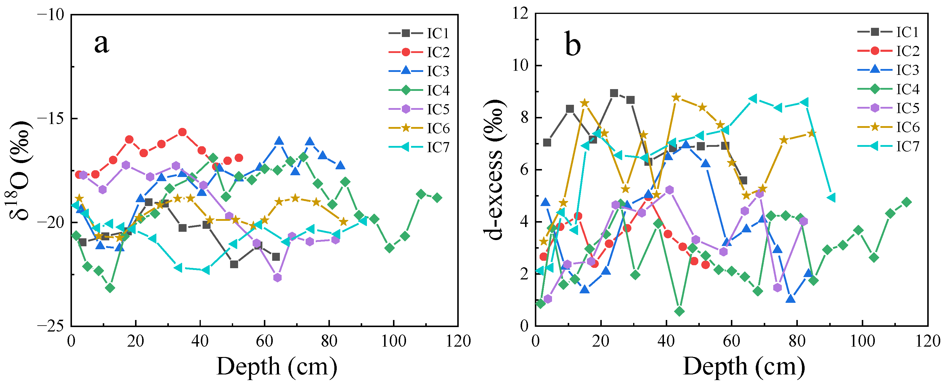
The variation trends of stable water isotopes (δ18O and δD) of ice cores are generally consistent with atmospheric temperature changes. As a result, stable water isotopes are often used as a proxy to indicate paleoclimate change. Meanwhile, stable water isotopes of ice cores have been used to compare with the grain size of ice cores [39,57]. Based on the global atmospheric precipitation line GMWL, excess deuterium (d-excess) can be defined as d-excess = Δd − 8 × δ18O [58]. The variations of stable isotopes of IC cores with depth are plotted in Figure 7. The stable water isotopes fluctuate with depth.
4. Discussion
4.1. Evolution and Spatial Variations of Ice Fabrics
The deformation-induced fabric has a deformation kinematic symmetry [59]. Most of the IC thin sections show a cluster fabric with two c-axis maximum orientations. The strength of the fabric is not obviously correlated with the variation in depth. The angle of the c-axis maximum evolves with depth at an angle within 10° in most cases. Double cluster fabrics have been observed in shear-dominated regimes where discontinuous dynamic recrystallization is active, both in experimental deformation tests [26,29] and in natural conditions [34,37,39]. Like what is shown in studies of Whillans [34], shear margin ice has coarse grains, irregular grain boundaries, and double-maximum c-axes orientations, which indicate that grain boundary migration is the dominant process. Meanwhile, force and morphological analyses of the cluster fabric were also performed in the ice radar-sounding study [60]. The fabric of basal ice shows one or two c-axis maximums and has a significant difference between each ice core.
Although the fabric of ice cores is weak in many thin sections, there still exists an evolution trend of ice fabric even within a small scale of 1 m depth. Therefore, in fabric studies of deeper ice cores, especially in areas with fast ice flow velocity, there may be potential uncertainties using ice samples at an interval of tens or hundreds of meters. As a result, we should be more careful about the variations of ice fabric within a small depth scale when explaining the fabric evolution mechanism. It is suggested that when studying critical depth zones of deep ice cores, continuous thin section sampling of several meters should be conducted to analyze the evolution of fabric.
4.2. Depth and Spatial Variations of Grain Size of IC Ice Cores
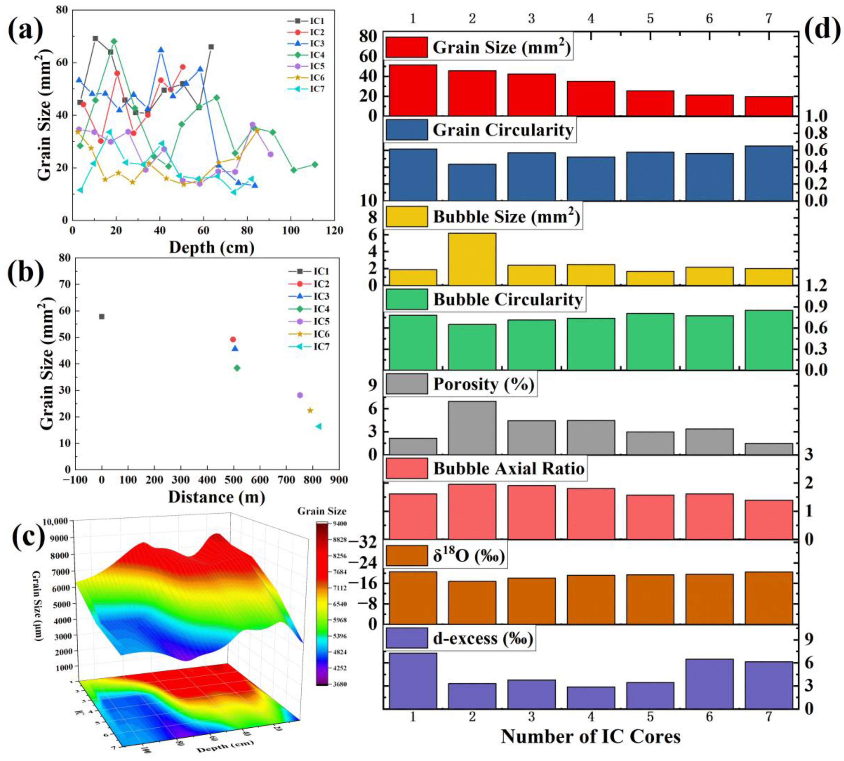
Figure 8a shows the variations of IC grain sizes with depth. As shown in Figure 8a, the grain size of each ice core fluctuates with the increase in depth. Variations of averaged grain sizes with the relative distances among different IC ice cores are shown in Figure 8b. The averaged proxies of each IC ice core, including grain size, grain circularity, bubble size, bubble circularity, porosity, bubble axial ratio, δ18O, and d-excess, are shown in Figure 8d. From Figure 8d, it can be seen that the grain size of the seven IC ice cores shows a decreasing trend. It is further shown in Figure 8b that the decreasing rate of grain size from IC2 to IC4 ice cores is relatively fast, and the decreasing rate of grain size from IC5 to IC7 ice cores is relatively slow. The decreasing rates of grain size with distance are 0.71 mm2/m from IC2 to IC4 and 0.16 mm2/m from IC5 to IC7. These two sets of ice cores correspond to two different shear margin sites of exposed bedrock, and both decreasing rates of grain size are faster than that from IC1 to IC2 (0.012 mm2/m).
Figure 8c shows a 3D-smooth projection of grain size to depth and ice flow (expressed by the number of IC ice cores). The smoothing method is adjacent-averaging with a smoothing parameter of 0.05 and a growth factor of 100. As shown in Figure 8c, the overall trend of grain size decreases with the increase in depth. The overall trend of grain size decreases as the ice cores get closer to the exposed bedrock. This result coincides with what we find in Figure 8b. In summary, the subglacial topography has a significant influence on the grain size in shallow glaciers at the shear margin.
4.3. Depth and Spatial Variations of Bubble Size of IC Ice Cores
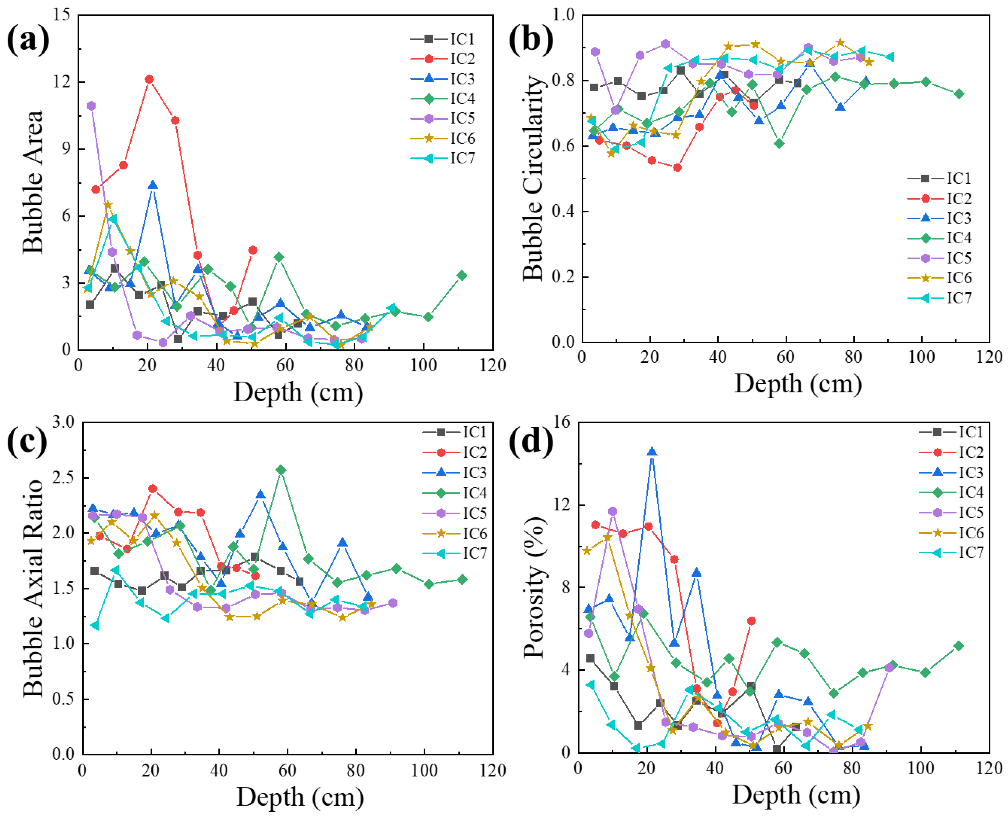
During the process of densification, snow and firn transform into ice and trap the air into bubbles. Blue ice areas at the margin of the ice sheet are usually in ablation zones, and the surface layers of the glacier are denuded in the summer season [61]. Variations of bubble size, circularity, axial ratio, and porosity with depth are shown in Figure 9. With the increase in depth, the bubble size decreases, and the bubble circularity increases.
According to the bubble size data of IC ice cores shown in Figure 8, the bubble sizes of IC1, IC3, and IC7 fluctuate around 2 mm2, while the bubble size of the IC2 ice core is much larger than all the other six ice cores, up to 6.177 mm2. It is shown in Figure 9 that at the shear margin of the Dalk Glacier, the bubbles become smaller and rounder, with increasing depth from the surface to 1 m-depth ice layer.
It is worth noting that this study is based on 2D thin sections for bubble analysis, which simplifies the 3D ice morphology. As a result, the original bubble characteristics in the 3D world are simplified into 2D profiles.
4.4. The Mechanism of the Formation of Shallow Bubble Tunnels
The bubble morphology of the IC ice cores shows that there are strip-shaped bubble channels in the shallow ice. Moreover, compared with the IC1 sample, IC2–IC7 contains more bubbles with larger bubble areas and longer bubble long-axis lengths. From the microscopic images and bubble area statistics, it is clear that the bubble channels are mostly distributed at the location of ice crystal boundaries. There are two possible reasons for the formation of shallow bubble channels. Firstly, the temperature of the surface layer of blue ice increases due to solar radiation in summer. Melting and denudation of the topmost ice layers can occur, and the increase in surface temperature leads to the increase in ice grain size, movement, and connection of bubbles. Even refreezing of the surface ice occurs, leading to the formation of larger bubble channels. Secondly, as the glacier flows, the deeper blue ice is lifted to the surface by the subglacial topography, the bubble size increases to release pressure, and bubble channels form.
By comparing the studies on ice samples with melting and refreezing interference [36], it shows that the grain sizes are larger if there is melting and refreezing. As shown in Figure 8a, the grain sizes of the shallowest ice layers are not obviously larger than the deeper layers. As a result, ablation but no refreezing happens to surface ice layers in this region. In addition, microstructure and fabric studies of shear margin ice of the Taylor Glacier [35] and the subsequent dating and studies on blue ice [62,63,64,65] show that blue ice from deep layers of ice sheet flows towards the exposed bedrock and forms the Taylor Glacier shear margin. It can be inferred that in this study, the blue ice layer flows from the original accumulation area and is uplifted by the bedrock to the surface. In conclusion, under the influence of ablation and bubble pressure release, the ice surface is denudated and bubble channels form in shallow ice layers.
4.5. Characteristics and Formation Mechanisms of Basal Ice Cores
As shown in Figure 10, the grain size of OIW ice cores is smaller than that of IW ice cores, especially for OIW1–OIW6. This results from the different properties between the ice layers since IW and OIW ice cores were drilled at two different sites according to Figure 1. Combined with the fact that the grain circularity of OIW is also smaller than that of IW ice cores, it can be concluded that OIW ice cores experience much more basal sliding and the grains were sheared into small and elongated properties. Meanwhile, this finding also coincides with the SPO properties. As shown in Figure 6, the SPOs of bubbles are in the same direction with the SPOs of grains in OIW ice cores. It means that bubbles and grains of OIW ice cores are stretched in the same direction by the shear stress conducted by the bedrock during glacier movement. There is intense friction and shear stress between the OIW basal ice and the bedrock. Since the ice cores are drilled horizontally, the grains and bubbles are stretched in the direction of the ice flow.
4.6. Correlations between Stable Water Isotopes and Grain Size
In studies of deep ice cores, grain size correlates with stable water isotopes in some cases to reveal layer information, such as folded ice layers [57]. For shallow ice cores at shear margins, conditions are more complicated due to ice flow and the influence of bedrock. The correlation between the IC1–IC7 ice core stable water isotope δ18O and grain size with depth is shown in Figure 11. It can be seen from the figure that, except for IC7, the stable water isotope δ18O has a weak negative correlation trend with the grain size of the other six ice cores. In this study, the grain size and stable water isotope of the ice cores fluctuate with depth. The seasonal/interannual variations of the original accumulation region are still preserved after the ice migrated to the surface shear margin. As shown in Figure 8d, the stable isotope δ18O decreases from IC2 to IC7, which is in positive correlation with the decrease in grain size, contrary to the findings in depth variations. Combined with the information we have found in the previous sections, it can be concluded that bedrock topography and shear stress have a greater influence on grain size than stable isotope δ18O among different ice cores over long distances. More studies are needed to further investigate the correlation between ice fabric and chemical proxies.
5. Conclusions
In this study, we investigated the fabric, microstructure, and stable water isotope of ice cores from the shear margin of the Dalk Glacier, Antarctica. Based on the analysis and comparison of the depth and spatial variations of these proxies, we evaluated the properties and formation mechanisms of the ice layers in this region. The conclusions are as follows:
1. This study shows that the ice cores at the shear margin of the Dalk Glacier mostly have a cluster fabric. There exist rotations of the c-axis maximum and fabric evolution in the shallow ice layer at a depth of 1 m;
2. The formation mechanism of blue ice in this study region is that the ice from the original accumulation area flows to these sites, then it is lifted to the surface by the subglacial bedrock and shaped by the influence of summer ablation and denudation;
3. Spatial variations of ice grain size show that the grain size becomes smaller as the ice cores get closer to the exposed bedrock. This means that the blocking and squeezing of the bedrock topography have a significant influence on the ice microstructure;
4. The basal ice at the glacier shear margin was strongly affected by the intense friction of the bedrock during the glacial movement. The basal ice mostly shows a cluster fabric, with one or two c-axis maximums. Ice grains and bubbles have a very strong shear-stretching characteristic in one of the basal sites;
5. With the increase in depth, the grain size of shallow ice cores has a weak negative correlation with the stable water isotope. Bedrock topography and shear stress have a greater influence on grain microstructure among different ice cores over long distances at shear margins.
The conclusions of this paper can help understand the properties of shallow and basal ice at the shear margins of the East Antarctic ice sheet and provide a reference for improving the Antarctic ice flow model. Admittedly, there are limitations to this paper. The relative directions between each ice sample and the ice flow were not well recorded when drilling in the field. Studies on more proxies of deeper ice cores are needed in the future to better understand the properties of blue ice at the shear margin of the Antarctic ice sheet.
Author Contributions
Conceptualization, S.L., D.W. and G.S.; investigation, S.L., D.W., T.M. and C.A.; methodology, S.L.; data curation, S.L.; writing—original draft, S.L.; writing—review and editing, N.Z., G.S., T.M., H.M. and Y.L.; funding acquisition, N.Z., G.S., T.M. and H.M. All authors have read and agreed to the published version of the manuscript.
Funding
This research was funded by the National Natural Science Foundation of China (No. 42176232, 41876225, 42276243, 41922046) and the Fundamental Research Funds for the Central Universities (WK2080000161).
Data Availability Statement
The data presented in this study are available upon request from the first author.
Acknowledgments
The authors are grateful to the members of the 36th CHINARE members for technical support and assistance. The authors thank the editor and anonymous reviewers for their valuable comments and suggestions to this paper.
Conflicts of Interest
The authors declare no conflict of interest.
References
- Willis, J.K.; Church, J.A. Regional Sea-Level Projection. Science 2012, 336, 550–551. [Google Scholar] [CrossRef] [PubMed]
- Gregory, J.M.; White, N.J.; Church, J.A.; Bierkens, M.F.P.; Box, J.E.; den Broeke, M.R.; Cogley, J.G.; Fettweis, X.; Hanna, E.; Huybrechts, P.; et al. Twentieth-Century Global-Mean Sea Level Rise: Is the Whole Greater than the Sum of the Parts? J. Clim. 2013, 26, 4476–4499. [Google Scholar] [CrossRef]
- Shepherd, A.; Fricker, H.A.; Farrell, S.L. Trends and connections across the Antarctic cryosphere. Nature 2018, 558, 223–232. [Google Scholar] [CrossRef] [PubMed]
- Goodman, D.J.; Frost, H.J.; Ashby, M.F. The plasticity of polycrystalline ice. Philos. Mag. A 1981, 43, 665–695. [Google Scholar] [CrossRef]
- Alley, R.B. Flow-law Hypotheses for Ice-Sheet Modeling. J. Glaciol. 1992, 38, 245–256. [Google Scholar] [CrossRef]
- Faria, S.H.; Weikusat, I.; Azuma, N. The microstructure of polar ice. Part II: State of the art. J. Struct. Geol. 2014, 61, 21–49. [Google Scholar] [CrossRef]
- Hunter, N.J.R.; Wilson, C.J.L.; Luzin, V. Crystallographic preferred orientation (CPO) patterns in uniaxially compressed deuterated ice: Quantitative analysis of historical data. J. Glaciol. 2022, 1–12. [Google Scholar] [CrossRef]
- Marshall, S.J. Recent advances in understanding ice sheet dynamics. Earth Planet. Sci. Lett. 2005, 240, 191–204. [Google Scholar] [CrossRef]
- Aster, R.C.; Winberry, J.P. Glacial seismology. Rep. Prog. Phys. 2017, 80, 126801. [Google Scholar] [CrossRef]
- Feldmann, J.; Reese, R.; Winkelmann, R.; Levermann, A. Shear-margin melting causes stronger transient ice discharge than ice-stream melting in idealized simulations. Cryosphere 2022, 16, 1927–1940. [Google Scholar] [CrossRef]
- Hudleston, P.J. Progressive Deformation and Development of Fabric Across Zones of Shear in Glacial Ice. In Energetics of Geological Processes: Hans Ramberg on His 60th Birthday; Saxena, S.K., Bhattacharji, S., Annersten, H., Stephansson, O., Eds.; Springer: Berlin/Heidelberg, Germany, 1977; pp. 121–150. [Google Scholar]
- Budd, W.F.; Jacka, T.H. A review of ice rheology for ice sheet modelling. Cold Reg. Sci. Technol. 1989, 16, 107–144. [Google Scholar] [CrossRef]
- Duval, P.; Montagnat, M.; Grennerat, F.; Weiss, J.; Meyssonnier, J.; Philip, A. Creep and plasticity of glacier ice: A material science perspective. J. Glaciol. 2010, 56, 1059–1068. [Google Scholar] [CrossRef]
- Montagnat, M.; Buiron, D.; Arnaud, L.; Broquet, A.; Schlitz, P.; Jacob, R.; Kipfstuhl, S. Measurements and numerical simulation of fabric evolution along the Talos Dome ice core, Antarctica. Earth Planet. Sci. Lett. 2012, 357–358, 168–178. [Google Scholar] [CrossRef]
- Lipenkov, V.Y.; Barkov, N.I.; Duval, P.; Pimienta, P. Crystalline Texture of the 2083 m Ice Core at Vostok Station, Antarctica. J. Glaciol. 1989, 35, 392–398. [Google Scholar] [CrossRef]
- Azuma, N.; Wang, Y.; Yoshida, Y.; Narita, H.; Hondoh, T.; Shoji, H.; Watanabe, O. Crystallographic analysis of the Dome Fuji ice core. In Physics of Ice Core Records; Hokkaido University Press: Sapporo, Japan, 2000; pp. 45–61. [Google Scholar]
- Durand, G.; Svensson, A.; Persson, A.; Gagliardini, O.; Gillet-Chaulet, F.; Sjolte, J.; Montagnat, M.; Dahl-Jensen, D. Evolution of the texture along the EPICA Dome C ice core. Low Temp. Sci. 2009, 68, 91–105. [Google Scholar]
- Weikusat, I.; Kipfstuhl, S.; Azuma, N.; Faria, S.H.; Miyamoto, A. Deformation Microstructures in an Antarctic Ice Core (EDML) and in Experimentally Deformed Artificial Ice. Low Temp. Sci. 2009, 68, 115–123. [Google Scholar]
- Faria, S.H.; Weikusat, I.; Azuma, N. The microstructure of polar ice. Part I: Highlights from ice core research. J. Struct. Geol. 2014, 61, 2–20. [Google Scholar] [CrossRef]
- Bamber, J.L.; Vaughan, D.G.; Joughin, I. Widespread Complex Flow in the Interior of the Antarctic Ice Sheet. Science 2000, 287, 1248–1250. [Google Scholar] [CrossRef] [PubMed]
- Bennett, M.R. Ice streams as the arteries of an ice sheet: Their mechanics, stability and significance. Earth-Sci. Rev. 2003, 61, 309–339. [Google Scholar] [CrossRef]
- Rignot, E.; Mouginot, J.; Scheuchl, B. Ice Flow of the Antarctic Ice Sheet. Science 2011, 333, 1427–1430. [Google Scholar] [CrossRef]
- Echelmeyer, K.A.; Harrison, W.D.; Larsen, C.; Mitchell, J.E. The role of the margins in the dynamics of an active ice stream. J. Glaciol. 1994, 40, 527–538. [Google Scholar] [CrossRef]
- Hruby, K.; Gerbi, C.; Koons, P.; Campbell, S.; Martín, C.; Hawley, R. The impact of temperature and crystal orientation fabric on the dynamics of mountain glaciers and ice streams. J. Glaciol. 2020, 66, 755–765. [Google Scholar] [CrossRef]
- Kamb, W.B. Experimental Recrystallization of Ice Under Stress. In Flow and Fracture of Rocks; Geophysical Monograph Series; California Institute of Technology: Pasadena, CA, USA, 1972; pp. 211–241. [Google Scholar]
- Bouchez, J.-L.; Duval, P. The Fabric of Polycrystalline Ice Deformed in Simple Shear: Experiments in Torsion, Natural Deformation and Geometrical Interpretation. Textures Microstruct. 1982, 5, 171–190. [Google Scholar] [CrossRef]
- Jun, L.; Jacka, T.H.; Budd, W.F. Strong single-maximum crystal fabrics developed in ice undergoing shear with unconstrained normal deformation. Ann. Glaciol. 2000, 30, 88–92. [Google Scholar] [CrossRef]
- Journaux, B.; Chauve, T.; Montagnat, M.; Tommasi, A.; Barou, F.; Mainprice, D.; Gest, L. Recrystallization processes, microstructure and crystallographic preferred orientation evolution in polycrystalline ice during high-temperature simple shear. Cryosphere 2019, 13, 1495–1511. [Google Scholar] [CrossRef]
- Qi, C.; Prior, D.J.; Craw, L.; Fan, S.; Llorens, M.G.; Griera, A.; Negrini, M.; Bons, P.D.; Goldsby, D.L. Crystallographic preferred orientations of ice deformed in direct-shear experiments at low temperatures. Cryosphere 2019, 13, 351–371. [Google Scholar] [CrossRef]
- Lawson, W.J.; Sharp, M.J.; Hambrey, M.J. The structural geology of a surge-type glacier. J. Struct. Geol. 1994, 16, 1447–1462. [Google Scholar] [CrossRef]
- Harrison, W.D.; Echelmeyer, K.A.; Larsen, C.F. Measurement of temperature in a margin of Ice Stream B, Antarctica: Implications for margin migration and lateral drag. J. Glaciol. 1998, 44, 615–624. [Google Scholar] [CrossRef]
- Barnes, P.R.F.; Wolff, E.W. Distribution of soluble impurities in cold glacial ice. J. Glaciol. 2004, 50, 311–324. [Google Scholar] [CrossRef]
- Pettit, E.C.; Whorton, E.N.; Waddington, E.D.; Sletten, R.S. Influence of debris-rich basal ice on flow of a polar glacier. J. Glaciol. 2014, 60, 989–1006. [Google Scholar] [CrossRef]
- Jackson, M.; Kamb, B. The marginal shear stress of Ice Stream B, West Antarctica. J. Glaciol. 1997, 43, 415–426. [Google Scholar] [CrossRef]
- Samyn, D.; Svensson, A.; Fitzsimons, S. Dynamic implications of discontinuous recrystallization in cold basal ice: Taylor Glacier, Antarctica. J. Geophys. Res. 2008, 113, F03S90. [Google Scholar] [CrossRef] [Green Version]
- Gerbi, C.; Mills, S.; Clavette, R.; Campbell, S.; Bernsen, S.; Clemens-Sewall, D.; Lee, I.; Hawley, R.; Kreutz, K.; Hruby, K. Microstructures in a shear margin: Jarvis Glacier, Alaska. J. Glaciol. 2021, 67, 1163–1176. [Google Scholar] [CrossRef]
- Monz, M.E.; Hudleston, P.J.; Prior, D.J.; Michels, Z.; Fan, S.; Negrini, M.; Langhorne, P.J.; Qi, C. Full crystallographic orientation (c and a axes) of warm, coarse-grained ice in a shear-dominated setting: A case study, Storglaciären, Sweden. Cryosphere 2021, 15, 303–324. [Google Scholar] [CrossRef]
- Hellmann, S.; Kerch, J.; Weikusat, I.; Bauder, A.; Grab, M.; Jouvet, G.; Schwikowski, M.; Maurer, H. Crystallographic analysis of temperate ice on Rhonegletscher, Swiss Alps. Cryosphere 2021, 15, 677–694. [Google Scholar] [CrossRef]
- Thomas, R.E.; Negrini, M.; Prior, D.J.; Mulvaney, R.; Still, H.; Bowman, M.H.; Craw, L.; Fan, S.; Hubbard, B.; Hulbe, C.; et al. Microstructure and Crystallographic Preferred Orientations of an Azimuthally Oriented Ice Core from a Lateral Shear Margin: Priestley Glacier, Antarctica. Front. Earth Sci. 2021, 9. [Google Scholar] [CrossRef]
- Bentley, C.R. Seismic-wave velocities in anisotropic ice: A comparison of measured and calculated values in and around the deep drill hole at Byrd Station, Antarctica. J. Geophys. Res. 1972, 77, 4406–4420. [Google Scholar] [CrossRef]
- Kohnen, H.; Gow, A.J. Ultrasonic Velocity Investigations of Crystal Anisotropy in Deep Ice Cores from Antarctica. J. Geophys. Res. -Ocean. Atmos. 1979, 84, 4865–4874. [Google Scholar] [CrossRef]
- Harland, S.R.; Kendall, J.M.; Stuart, G.W.; Lloyd, G.E.; Baird, A.F.; Smith, A.M.; Pritchard, H.D.; Brisbourne, A.M. Deformation in Rutford Ice Stream, West Antarctica: Measuring shear-wave anisotropy from icequakes. Ann. Glaciol. 2013, 54, 105–114. [Google Scholar] [CrossRef]
- Smith, E.C.; Baird, A.F.; Kendall, J.M.; Martín, C.; White, R.S.; Brisbourne, A.M.; Smith, A.M. Ice fabric in an Antarctic ice stream interpreted from seismic anisotropy. Geophys. Res. Lett. 2017, 44, 3710–3718. [Google Scholar] [CrossRef]
- Jordan, T.M.; Schroeder, D.M.; Elsworth, C.W.; Siegfried, M.R. Estimation of ice fabric within Whillans Ice Stream using polarimetric phase-sensitive radar sounding. Ann. Glaciol. 2020, 61, 74–83. [Google Scholar] [CrossRef]
- Lutz, F.; Eccles, J.; Prior, D.J.; Craw, L.; Fan, S.; Hulbe, C.; Forbes, M.; Still, H.; Pyne, A.; Mandeno, D. Constraining Ice Shelf Anisotropy Using Shear Wave Splitting Measurements from Active-Source Borehole Seismics. J. Geophys. Res. Earth Surf. 2020, 125, e2020JF005707. [Google Scholar] [CrossRef]
- Hellmann, S.; Grab, M.; Kerch, J.; Löwe, H.; Bauder, A.; Weikusat, I.; Maurer, H. Acoustic velocity measurements for detecting the crystal orientation fabrics of a temperate ice core. Cryosphere 2021, 15, 3507–3521. [Google Scholar] [CrossRef]
- Rathmann, N.M.; Lilien, D.A.; Grinsted, A.; Gerber, T.A.; Young, T.J.; Dahl-Jensen, D. On the Limitations of Using Polarimetric Radar Sounding to Infer the Crystal Orientation Fabric of Ice Masses. Geophys. Res. Lett. 2022, 49, e2021GL096244. [Google Scholar] [CrossRef]
- Shugar, D.H.; Jacquemart, M.; Shean, D.; Bhushan, S.; Upadhyay, K.; Sattar, A.; Schwanghart, W.; McBride, S.; de Vries, M.V.W.; Mergili, M.; et al. A massive rock and ice avalanche caused the 2021 disaster at Chamoli, Indian Himalaya. Science 2021, 373, 300–306. [Google Scholar] [CrossRef] [PubMed]
- Smedley, A.R.D.; Evatt, G.W.; Mallinson, A.; Harvey, E. Solar radiative transfer in Antarctic blue ice: Spectral considerations, subsurface enhancement, inclusions, and meteorites. Cryosphere 2020, 14, 789–809. [Google Scholar] [CrossRef]
- Muhuri, A.; Manickam, S.; Bhattacharya, A.; Snehmani. Snow Cover Mapping Using Polarization Fraction Variation With Temporal RADARSAT-2 C-Band Full-Polarimetric SAR Data Over the Indian Himalayas. IEEE J. Sel. Top. Appl. Earth Obs. Remote Sens. 2018, 11, 2192–2209. [Google Scholar] [CrossRef]
- Tsai, Y.-L.S.; Dietz, A.J.; Oppelt, N.; Kuenzer, C. Remote Sensing of Snow Cover Using Spaceborne SAR: A Review. Remote. Sens. 2019, 11, 1456. [Google Scholar] [CrossRef]
- Qiao, H.; Zhang, P.; Li, Z.; Liu, C. A New Geostationary Satellite-Based Snow Cover Recognition Method for FY-4A AGRI. IEEE J. Sel. Top. Appl. Earth Obs. Remote Sens. 2021, 14, 11372–11385. [Google Scholar] [CrossRef]
- Wilson, C.J.L.; Russell-Head, D.S.; Kunze, K.; Viola, G. The analysis of quartz c-axis fabrics using a modified optical microscope. J. Microsc. 2007, 227, 30–41. [Google Scholar] [CrossRef]
- Legland, D.; Arganda-Carreras, I.; Andrey, P. MorphoLibJ: Integrated library and plugins for mathematical morphology with ImageJ. Bioinformatics 2016, 32, 3532–3534. [Google Scholar] [CrossRef]
- Schindelin, J.E.; Arganda-Carreras, I.; Frise, E.; Kaynig, V.; Longair, M.; Pietzsch, T.; Preibisch, S.; Rueden, C.T.; Saalfeld, S.; Schmid, B.; et al. Fiji: An open-source platform for biological-image analysis. Nat. Methods 2012, 9, 676–682. [Google Scholar] [CrossRef] [Green Version]
- Arganda-Carreras, I.; Kaynig, V.; Rueden, C.; Eliceiri, K.W.; Schindelin, J.; Cardona, A.; Sebastian Seung, H. Trainable Weka Segmentation: A machine learning tool for microscopy pixel classification. Bioinformatics 2017, 33, 2424–2426. [Google Scholar] [CrossRef]
- Montagnat, M.; Azuma, N.; Dahl-Jensen, D.; Eichler, J.; Fujita, S.; Gillet-Chaulet, F.; Kipfstuhl, S.; Samyn, D.; Svensson, A.; Weikusat, I. Fabric along the NEEM ice core, Greenland, and its comparison with GRIP and NGRIP ice cores. Cryosphere 2014, 8, 1129–1138. [Google Scholar] [CrossRef]
- Dansgaard, W. Stable isotopes in precipitation. Tellus 1964, 16, 436–468. [Google Scholar] [CrossRef]
- Wenk, H.R.; Christie, J.M. Comments on the interpretation of deformation textures in rocks. J. Struct. Geol. 1991, 13, 1091–1110. [Google Scholar] [CrossRef]
- Young, T.J.; Schroeder, D.M.; Jordan, T.M.; Christoffersen, P.; Tulaczyk, S.M.; Culberg, R.; Bienert, N.L. Inferring Ice Fabric From Birefringence Loss in Airborne Radargrams: Application to the Eastern Shear Margin of Thwaites Glacier, West Antarctica. J. Geophys. Res. Earth Surf. 2021, 126, e2020JF006023. [Google Scholar] [CrossRef]
- Cuffey, K.; Paterson, W. The Physics of Glaciers, 4th ed.; Butterworth-Heinemann: Oxford, UK, 2010; pp. 11–28. [Google Scholar]
- Buizert, C.; Baggenstos, D.; Jiang, W.; Purtschert, R.; Petrenko, V.V.; Lu, Z.T.; Muller, P.; Kuhl, T.; Lee, J.; Severinghaus, J.P.; et al. Radiometric Kr 81 dating identifies 120,000-year-old ice at Taylor Glacier, Antarctica. Proc. Natl. Acad. Sci. USA 2014, 111, 6876–6881. [Google Scholar] [CrossRef]
- Bauska, T.K.; Baggenstos, D.; Brook, E.J.; Mix, A.C.; Marcott, S.A.; Petrenko, V.V.; Schaefer, H.; Severinghaus, J.P.; Lee, J.E. Carbon isotopes characterize rapid changes in atmospheric carbon dioxide during the last deglaciation. Proc. Natl. Acad. Sci. USA 2016, 113, 3465–3470. [Google Scholar] [CrossRef]
- Baggenstos, D.; Bauska, T.K.; Severinghaus, J.P.; Lee, J.E.; Schaefer, H.; Buizert, C.; Brook, E.J.; Shackleton, S.; Petrenko, V.V. Atmospheric gas records from Taylor Glacier, Antarctica, reveal ancient ice with ages spanning the entire last glacial cycle. Clim. Past 2017, 13, 943–958. [Google Scholar] [CrossRef]
- Menking, J.A.; Brook, E.J.; Shackleton, S.A.; Severinghaus, J.P.; Dyonisius, M.N.; Petrenko, V.; McConnell, J.R.; Rhodes, R.H.; Bauska, T.K.; Baggenstos, D.; et al. Spatial pattern of accumulation at Taylor Dome during Marine Isotope Stage 4: Stratigraphic constraints from Taylor Glacier. Clim. Past 2019, 15, 1537–1556. [Google Scholar] [CrossRef] [Green Version]
Figure 1.
Maps of the drilling sites. (a) Map of Antarctica; (b) map of Dalk Glacier region; (c) map of the drill sites of the ice cores (the blue arrow represents the direction of ice flow); (d) drill sites of IW ice cores; (e) drill sites of OIW ice cores; (f) IW1-IW3; (g) IW4-IW6; (h) IW7; (i) OIW1-OIW3; (j) OIW4-OIW6; (k) OIW7-OIW9.

Figure 2.
Microstructure maps of thin sections. (a) IC1-1; (b) IC1-2; (c) IC1-9; (d) IC1-10; (e) IC3-1; (f) IC3-2; (g) IC3-12; (h) IC3-13; (i) IW5; (j) OIW5.
Figure 2.
Microstructure maps of thin sections. (a) IC1-1; (b) IC1-2; (c) IC1-9; (d) IC1-10; (e) IC3-1; (f) IC3-2; (g) IC3-12; (h) IC3-13; (i) IW5; (j) OIW5.

Figure 3.
(a) The Schmidt diagrams (equatorial projections of c-axis orientations), each point represents the c-axis orientation of each grain; (b) the kernel contour maps of c-axis orientations of ice, the density of c-axes represents the strength of the fabric; (c) the microstructure maps with colored orientations of each grain, the legend of the map is shown in the color wheel at the top left of Figure 3. The left side shows the basic information for each thin section, including sample number, depth (D), and number of c-axis (N), one c-axis per grain.


Figure 4.
Grain frequency distribution diagrams. ‘D’ means depth, ‘N’ means number of grains. (a) Frequency distributions of grain size (mm2); (b) frequency distributions of grain circularity; (c) frequency distributions of grain ellipse elongation.
Figure 4.
Grain frequency distribution diagrams. ‘D’ means depth, ‘N’ means number of grains. (a) Frequency distributions of grain size (mm2); (b) frequency distributions of grain circularity; (c) frequency distributions of grain ellipse elongation.


Figure 5.
Bubble frequency distribution diagrams. ‘D’ means depth, ‘n’ means number of bubbles. (a) Frequency distributions of bubble size (mm2); (b) frequency distributions of bubble circularity; (c) frequency distributions of bubble axial ratio.
Figure 5.
Bubble frequency distribution diagrams. ‘D’ means depth, ‘n’ means number of bubbles. (a) Frequency distributions of bubble size (mm2); (b) frequency distributions of bubble circularity; (c) frequency distributions of bubble axial ratio.


Figure 6.
(a) Rose diagrams of shape-preferred orientations of ice grains; (b) rose diagrams of shape-preferred orientations of bubbles. ‘D’ means depth of the sample.
Figure 6.
(a) Rose diagrams of shape-preferred orientations of ice grains; (b) rose diagrams of shape-preferred orientations of bubbles. ‘D’ means depth of the sample.

Figure 7.
(a) Variations of δ18O with depth of IC ice cores; (b) variations of d-excess with depth of IC ice cores.
Figure 7.
(a) Variations of δ18O with depth of IC ice cores; (b) variations of d-excess with depth of IC ice cores.

Figure 8.
(a) Variations of IC grain sizes with depth; (b) variations of averaged grain sizes with the relative distances among different IC ice cores; (c) 3D smooth surface projection of grain size (μm), sample number and depth (cm). Grain size is the equivalent diameter corresponding to the grain average area. Smoothing method is adjacent-averaging, smoothing parameter is 0.05, total growth factor is 100; (d) averaged proxies of each IC core including grain size, grain circularity, bubble size, bubble circularity, porosity, bubble axial ratio, δ18O, and d-excess.

Figure 9.
(a) Variations of bubble size with depth; (b) variations of bubble circularity with depth; (c) variations of bubble axial ratio with depth; (d) variations of porosity with depth.
Figure 9.
(a) Variations of bubble size with depth; (b) variations of bubble circularity with depth; (c) variations of bubble axial ratio with depth; (d) variations of porosity with depth.

Figure 10.
Grain and bubble characteristics of IW (I1-I7H) and OIW (O1–O9) ice cores. ‘H’ means horizontal thin sections, which cut perpendicularly to the drilling direction.
Figure 10.
Grain and bubble characteristics of IW (I1-I7H) and OIW (O1–O9) ice cores. ‘H’ means horizontal thin sections, which cut perpendicularly to the drilling direction.

Figure 11.
Correlations between ice grain sizes and stable water isotope δ18O.


Table 1.
Basic information of sampling sites.
| Name | Longitude (E) | Latitude (S) | Altitude (m) | Drilling Direction |
|---|---|---|---|---|
| IC1 | 76°20′17.78″ | 69°24′54.68″ | 143 | Vertical |
| IC2 | 76°20′25.05″ | 69°24′40.09″ | 139 | Vertical |
| IC3 | 76°20′25.03″ | 69°24′39.85″ | 139 | Vertical |
| IC4 | 76°20′24.79″ | 69°24′39.74″ | 143 | Vertical |
| IC5 | 76°20′31.89″ | 69°24′33.59″ | 159 | Vertical |
| IC6 | 76°20′32.46″ | 69°24′34.69″ | 161 | Vertical |
| IC7 | 76°20′32.59″ | 69°24′35.83″ | 161 | Vertical |
| IW1-IW3 | 76°20′28.23″ | 69°24′26.35″ | 27 | Horizontal |
| IW4-IW6 | 76°20′29.43″ | 69°24′25.50″ | 20 | Horizontal |
| IW7 | 76°20′24.69″ | 69°24′24.48″ | 19 | Horizontal |
| OIW1-OIW3 | 76°20′46.72″ | 69°24′29.55″ | 155 | Horizontal |
| OIW4-OIW6 | 76°20′46.87″ | 69°24′29.05″ | 151 | Horizontal |
| OIW7-OIW9 | 76°20′45.39″ | 69°24′28.23″ | 152 | Horizontal |
Disclaimer/Publisher’s Note: The statements, opinions and data contained in all publications are solely those of the individual author(s) and contributor(s) and not of MDPI and/or the editor(s). MDPI and/or the editor(s) disclaim responsibility for any injury to people or property resulting from any ideas, methods, instructions or products referred to in the content. |
© 2023 by the authors. Licensee MDPI, Basel, Switzerland. This article is an open access article distributed under the terms and conditions of the Creative Commons Attribution (CC BY) license (https://creativecommons.org/licenses/by/4.0/).
Share and Cite
MDPI and ACS Style
Lu, S.; Zhang, N.; Wang, D.; Shi, G.; Ma, T.; Ma, H.; An, C.; Li, Y. Spatial Variations of Fabric and Microstructure of Blue Ice Cores at the Shear Margin of Dalk Glacier, Antarctica. Water 2023, 15, 728. https://doi.org/10.3390/w15040728
AMA Style
Lu S, Zhang N, Wang D, Shi G, Ma T, Ma H, An C, Li Y. Spatial Variations of Fabric and Microstructure of Blue Ice Cores at the Shear Margin of Dalk Glacier, Antarctica. Water. 2023; 15(4):728. https://doi.org/10.3390/w15040728
Chicago/Turabian StyleLu, Siyu, Nan Zhang, Danhe Wang, Guitao Shi, Tianming Ma, Hongmei Ma, Chunlei An, and Yuansheng Li. 2023. "Spatial Variations of Fabric and Microstructure of Blue Ice Cores at the Shear Margin of Dalk Glacier, Antarctica" Water 15, no. 4: 728. https://doi.org/10.3390/w15040728
Note that from the first issue of 2016, this journal uses article numbers instead of page numbers. See further details here.