
How to Statistically Disentangle the Effects of Environmental Factors and Human Disturbances: A Review
1
Illinois Natural History Survey, Prairie Research Institute, University of Illinois, Champaign, IL 61820, USA
2
International Joint Commission, P.O. Box 32869, Detroit, MI 48232, USA
3
Institute for Fisheries Research, University of Michigan, Ann Arbor, MI 48109, USA
*
Author to whom correspondence should be addressed.
Water 2023, 15(4), 734; https://doi.org/10.3390/w15040734
Submission received: 16 January 2023
/
Revised: 7 February 2023
/
Accepted: 9 February 2023
/
Published: 13 February 2023
(This article belongs to the Special Issue Disentangling Influences of Natural and Human Factors on Aquatic Ecosystems)
Abstract
:Contemporary biological assemblage composition and biodiversity are often shaped by a range of natural environmental factors, human disturbances, and their interactions. It is critical to disentangle the effects of individual natural variables and human stressors in data analysis to support management decision-making. Many statistical approaches have been proposed and used to estimate the biological effects of individual predictors, which often correlated and interacted with one another. In this article, we review nine of those approaches in terms of their strengths, limitations, and related r packages. Among those are hierarchical partitioning, propensity score, the sum of AIC weights, structural equation modeling, and tree-based machine learning algorithms. As no approach is perfect, we offer two suggestions: (1) reducing the number of predictors as low as possible by carefully screening all candidate predictors based on biological and statistical considerations; (2) selecting two or more approaches based on the characteristics of the given dataset and specific research goals of a study, and using them in parallel or sequence. Our review could help ecologists to navigate through this challenging process.
1. Introduction
Natural environmental factors (e.g., climate and elevation) and human disturbances (e.g., land use, fine sediment, and mining) are often found to jointly affect species abundance and communities in survey-based studies. It is critical to identify the real effects of individual factors or groups of factors for understanding the environmental process and making management decisions. In a controlled experiment, the effect of different factors and their interactions can be estimated with a randomized block design [1,2]. However, such a design only can accommodate a small number of factors at relatively small scales of space and time. Most ecological processes operate at broad spatial and time scales, such as urbanization, agricultural practices, river damming, and climate changes, and are not possible to experiment with [3]. Ecological surveys and modeling based on field data are essential to infer or test hypothesized casual-effects relationships between environment and biological responses.
In practice, the statistical difficulty in disentangling the effects of individual environmental factors and human stressors mainly comes from two sources. First, different biotic and abiotic predictors often co-vary with one another in a given study. When the co-variation is linear, it is referred to as collinearity. When three or more predictors are linearly correlated with one another, it is referred to as multicollinearity. Collinearity occurs for a number of reasons, such as being different descriptors of the same ecological and physical process. For example, mean, max, and min monthly temperatures are often highly correlated because they all describe thermal regimes. Collinearity may also happen because of a causal-effect relationship. For example, both agricultural land use and natural environmental factors such as soil permeability and watershed slope affect aquatic biodiversity. They are also highly correlated as crops often grow better in watersheds of low slopes and permeable soil. Similarly, the elevation and % of forests in the watershed are also positively correlated because deforestation mainly occurs at low altitudes [4]. Nutrients, fine sediments, and water temperature can all be increased by agricultural land use [5]. Finally, environmental factors and disturbances simply co-vary by chance in some regions or over a given period. For example, climate (e.g., air temperature, precipitation), land use in the watershed, soil property, and depth of bedrock strongly co-vary with one another from North to South in Illinois, USA (Table 1, also see [6]), although such correlations may not hold at a broader scale.
Ignoring collinearity in data analysis can lead to many consequences [7]. First, the effect of a given factor can be misinterpreted. For example, species diversity and biological index values may be low at a site because of harsh natural environmental conditions, such as unstable flow and low productivity. Without accounting for the compounding effects of the natural factors, one may mistake the low values as an indication of degraded habitats and biological communities (Type II error). In contrast, species diversity and biological indices may be relatively high at a stream due to natural causes (e.g., larger stream size, rocky substrates, and close to a high-quality stream), and the site may be considered to be healthy, although it has been significantly compromised by human disturbances (Type I error). Similarly, low species diversity under a warm and wet climate may be interpreted as the effects of a warm and wet climate is negative without considering the positive correlation of climate with land use and geology [6]. In aquatic bioassessment, multiple stressors (e.g., nutrients, fine sediment, high temperature, and altered flow) often simultaneously affect biological communities [8,9]. It is critical to separate the impacts of stressors for management decisions. Misidentification of main anthropological stressors can be highly costly in both the economy and the environment. In ecological modeling, collinearity can lead to a large error in coefficient estimation, unstable performance, and difficulty in assessing predictor importance [7].
The second source of the difficulty is the fact that the effect of one predictor on the response variable may depend on other predictors, i.e., interactions. For example, the toxicity of a heavy metal to aquatic species is often dependent on pH, alkalinity, and other heavy metals [10], while the effect of dissolved oxygen varies with temperature and flow velocity [11]. The interactions further complicate our efforts to estimate the biological effect of a given environmental factor or human stressor. Most conventional statistical approaches require explicitly including interaction terms in a model, while some other methods may automatically account for interactions. When a large number of environmental variables are considered, the number of possible interactions is vast. It is important to identify significant interactions and take them into account in disentangling the effects of environmental factors and human disturbances.
Many statistical approaches have been used to separate the effects of different factors from one another (for typological approaches, see [12,13]). One can use those approaches to investigate a wide range of ecological responses. This review focuses on univariate response variables of biological communities, such as species diversity and multi-metric indices used for freshwater bioassessment [14,15]. The methods for the multivariate response, such as biological community composition, are only briefly discussed. We made two more restrictions to our review on this broad topic. First, reducing data redundancy is often the first step in statistical modeling. A variety of approaches are available, including correlation analysis, cluster analysis, variance inflation factor, and latent variables [7,16,17,18]. We shall not discuss those approaches (see [7] for review) but highlight the importance of ecological consideration for variable selection at the end of the article. Second, our review shall also exclude many commonly-used approaches to disentangling the effects of individual predictors, including averaging regression coefficients, regression of residuals, and stepwise regression. This is because these methods have been thoroughly reviewed and found to be often inadequate (see [19,20]). For example, the stepwise selection can lead to sub-optimal models, inflated R2, and the inclusion of random variables in a model [19]. In comparison, the regression of residuals tends to underestimate the effects of the targeted predictor, as the variance explained in the first regression is attributed to the co-variables alone [21]. Subsequently, we select nine approaches that are relatively new, promising but less used, commonly used but controversial, or specifically designed for freshwater studies. We review the concept, applications, potentials-limitations, and related r-packages for each of the approaches.
2. Modeling Based on Stratified Randomized Survey
Environmental variables and human stressors are often highly correlated with one another when sampling units are randomly selected. The best way to reduce the inter-correlation is probably through a proper study design. Redlich et al. [22] proposed a stratified randomization design to reduce or eliminate the collinearity among climate and land use variables. In this design, one first delineates a study region, then chooses strata for different spatial scales to create small spatial units, and finally randomly selects a set of spatial units that minimize the correlation between the predictor of interest and its co-variables. In Redlich et al. [22], the goal is to reduce the correlation between climate and regional land use and between the local habitat types and the edging effectsof habitats. Two strata are used at the regional scale, major land-use (three types, near-natural, agricultural, and urban), and climate (five zones) to create 15 combinations. Four quadrats (5.8 × 5.8 km) are then randomly chosen for each combination. This step keeps the correlation between land use and climate variables (temperature and precipitation) to be generally low (|r| < 0.3). At the landscape scale (1 km radius), the local habitat is used as the stratum (forests, grassland, arable land, and settlement). Each of the 60 quadrants selected is divided into grid cells of 320 × 320 m. The habitat composition and edging effect on vertebrate communities are calculated for a plot of a 1 km radius around the center of each 10,000 cells randomly selected for each quadrat selected. Then a subset of plots is selected to minimize the correlation between habitat and edging effects. The correlation between habitat composition and edging effect is substantially reduced compared with simple-random design. With much-reduced multicollinearity, a variety of statistical models can be applied, such as the generalized linear model (GLM.) or the Generalized Additive Model (GAM), to reliably estimate the effects of targeted predictors, i.e., the climate in this case.
The stratified random design has been successfully applied to a number of terrestrial studies on plants and arthropods [23,24,25]. It may be applied to aquatic studies to overcome the difficulty associated with multicollinearity, as shown in Table 1. However, how to incorporate stream networks into this design needs to be figured out because the environmental conditions (e.g., water temperature and nutrients) at a given stream site are strongly affected by environmental processes operating at the watershed level [26,27]. A more general challenge is that when applied to existing datasets, one may have to give up a large proportion of information available, such as species records or field samples, because their cells are not selected. This information loss may not be acceptable in many cases, particularly for rare species studies.
3. Structured Equation Model (SEM)
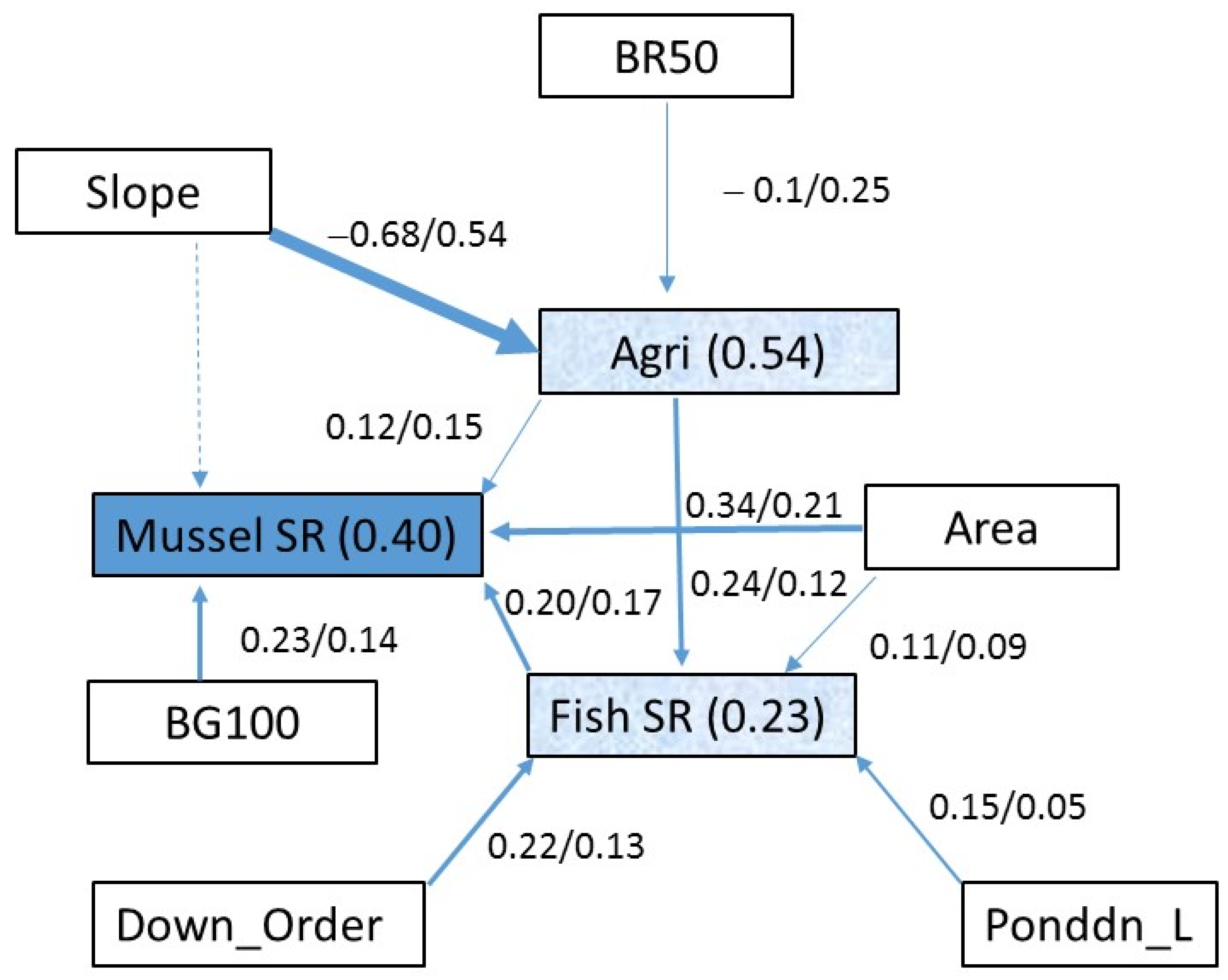
SEM unites multiple predictors and response variables in a single causal network. Two features distinguish it from other statistical models (e.g., GLM and GAM): (1) each path in the network represents an assumed or hypothesized relationship between a predictor and its response variables; (2) a response variable can be the predictor of other response variables. These features give SEM several advantages, such as testing multiple hypotheses simultaneously and accounting for measurement errors [28]. Thus, SEM is particularly powerful in disentangling the direct and indirect effects of predictors as well as cascade effects. For example, many natural environmental variables (e.g., surficial geology and watershed topography) affect mussel species directly and indirectly through land use and fish hosts [6,29]. In this case, land use and fish are the response variables of natural environmental factors and the predictors of mussel species diversity (Figure 1).
In SEM, each path is typically fitted with a linear model and tested for statistical significance. Interactions between predictors can be added as separate paths. Those insignificant paths are then removed. The causal network can be further simplified based on AIC. The model performance can be assessed based on a Chi-square test on the observed and predicted covariance matrix and the importance of each path based on the standardized regression coefficient. A number of r-packages are available to implement SEM, such as LAVAAN and sem. The approach has been applied to many freshwater studies [30]. The standard SEM is limited to linear regressions, and all paths have to be fit simultaneously, which is computationally demanding. A recent development, piecewise SEM [31] has extended the path fitting to GLM and fitting individually while the significance test of a path and AIC-based model selection remains applicable. A r-pacage, pSEM is used to perform this extended SEM. This extension also allows including the effect of auto-correlation, something that often compounds the effects of predictors. Several recent aquatic studies have successfully applied SEM or pSEM to assess the impacts of human disturbances on aquatic ecosystems [32,33,34].
There are a number of challenges in SEM [28]. Appropriately building of an SEM requires a thorough understanding of the study system and the establishment of a meaningful causal network. The number of possible paths rapidly increases with the number of predictors considered and thus needs to be carefully screened. Overly-complex networks are time-demanding to model and hard to interpret, while overly-simple networks can misrepresent the system and lead to poor model fitting. Nevertheless, SEM is a highly valuable tool for disentangling the effects of natural environmental factors and human disturbances.
4. Propensity Scores (PS)
In the real world, the predictor of interest (e.g., fine sediment loading) co-varies with many other predictors (e.g., water temperature, nutrients, stream slope, and flow). The propensity score is designed to cope with this difficulty. It is either the probability of treatment or the value of the targeted predictor conditioned upon all co-variables. The score is not observable, and it needs to be estimated with a model, such as logistic regression for binary treatment, GLM, or GAM. PS is then used to divide a whole dataset into subsets so that the co-variables are similar across sites of a subset and the effect of the targeted predictor can be more accurately estimated than based on the whole dataset [35].
Other propensity methods are available and may be more appropriate for a given study [36]. We here focus on the data matching method described above. After one divides all sampling sites into a number of bins based on the propensity scores, the correlation between the targeted predictor and other co-variables should be substantially reduced, and so is the compounding effects of the co-varaibles. The r-package, matchit is commonly used to implement this procedure. Other packages such as Matching, PSAgraphics, and twang are also available. Keller and Tipton [37] summarized and compared the features of these packages.
The propensity approach has been wildly used in social, economic, and epidemic studies but much less so in ecological studies [36]. Yuan [38] used it to estimate the effects of nutrients on stream macroinvertebrates with precipitation, watershed sizes, substrates, land cover, and several other environmental variables as co-variables and used GAM to estimate propensity scores. Similarly, Pearson et al. [39] used GLM to estimate propensity scores for nutrients with climate and geology as co-variables. More recently, Ramsey et al. [36] reviewed the concepts and different ways to use the propensity scores and demonstrated the efficiencies of the approach using both simulated and real data. In addition, the classification tree [40] and Random-forest regression [41] are also increasingly used for propensity scores in medical studies [42,43]. Both algorithms are commonly used in ecology and should help to boost the applications of the propensity scores in ecology.
One key assumption of propensity scores is all important co-variables are included in the modeling. This assumption may not always hold in practice because some co-variables may be unrecognized, unobservable, or unavailable. In the last two cases, surrogates, indices, or latent variables of these co-variables may be used to capture their effects to some extent. A number of other factors also could affect the effectiveness of the approach: (1) the size of datasets [36]; (2) the choice of modeling algorithms for propensity score estimation, and (3) the number of data bins [38]. The best choices for the last two factors are likely to be dataset-specific. One may need to try a number of algorithms and data-splitting schemes to maximize the model performance.
5. Hierarchical Partitioning (HP)
Hierarchical partitioning is a protocol to estimate the unique and joint effects of a predictor on the response variable based on GLM [44]. It was introduced into ecological studies by Mac Nally [19] The protocol starts with generating all possible models for n predictors. The goodness of fit can be measured with a number of measures, such as R2 for linear regression or χ2 for logistic regression. The unique effect is measured as the average increase in model fit across all models that contain the predictor of interest compared with the models without it. If the predictor has a high independent effect, the increase should be substantial, and vice versa. The averaging should alleviate the compounding effects [19]. Three steps are needed to estimate the joint effect. First, one calculates the goodness-of-fit for the model based on a predictor j alone as Rj, based on a subset of other predictors, e.g., l and k as Rlk, and based on all the predictors (j, l, k) as Rjlk. Second, the joint effect of predictor j with the given subset of predictors is calculated as (Rj + Rlk − Rjlk). Third, the joint effects for predictor j and all possible subsets of other predictors are averaged as the final estimate of predictor j. If a predictor is highly correlated with the response variable as well as with other predictors, the joint effect will be high; however, the unique effect will be low. As a result, the result may not be too informative. Thus, it is critical to reduce multicollinearity by selecting meaningful and relatively independent predictors at the first palce.
R-package, hier.part has been widely used to estimate the effects of different environmental variables in aquatic habitats (e.g., [45]). The package also offers a randomization test on the unique and joint effects and calculates the ratio between the unique and joint effects, which can be useful to assess the importance of a given predictor in ecosystem management [19,46]. Hierarchical partitioning is currently applicable to linear effects of up to 12 predictors (hier.part v1.06). However, a recent package, rdacca.hp, removes this limitation [47]. Lai et al. [48] further extended the approach to Generalized Linear Mixed Model (GLMM), which fits both fixed and random effects, with an R-package glmm.hp. However, this variance partitioning approach cannot handle non-linear responses and interactions among predictors, which are common in ecological studies. Olea et al. [49] also reported the order of predictors in the dataset could affect the relative importance of predictors when more than nine predictors are used and suggested multiple runs to assess the stability of the outcome. Smith et al. [20] found that hierarchical partitioning tended to underestimate the effect of predictors correlated with other variables but overestimated the effects of unrelated predictors. Warton [50] further criticized averaging R2 as its value is not comparable among different models. Users should be aware of these criticisms or weaknesses. Nevertheless, when used approperaitely, this approach is a valuable tool for ecologists.
6. Commonality Analysis (CA)
The commonality analysis approach was proposed in the late 1960s [51] and has been commonly used in social and psychological studies [52]. It was introduced to ecology much late but its application is increasing [46]. The basic idea is simple. One can estimate the R2 of a GLM based on n predictors and n − 1 predictors (predictor i is removed). The unique effect of predictor i will be the difference in R2 between the two models. The common effect will be estimated as R2 of the full model minus the unique effect of each predictor. Similarly, one can estimate the unique and common effects of any 2, 3, 4… n − 1 predictors. An r-package, yhat [53] can be used to implement this analysis.
When the number of predictors is controlled, this approach can provide valuable insights into the effects of different predictors. Ray-Mukherjee et al. [54] showed that a predictor might be correlated with other predictors but not the response variables; however, the predictor can help other predictors to estimate the response better. Such a predictor is likely dropped by some other approaches (e.g., correlation analysis). The use of this approach in ecology, particularly aquatic studies, is limited so far. However, a number of studies showed its usefulness. For example, Prunier et al. [55] used commonality analysis to estimate the effects of river network structure, stocking, and human stressors on the genetic diversity of two fish species, and they found that the first two factors played a much bigger role. Alahuhta et al. [56] used commonality analysis to compare the effects of local environments, climate, and geographic locations on lake macrophyte meta-communities and concluded that local environments drive the variation within meta-communities, but climate and geographic locations are influential for the variation across meta-communities.
This approach is similar to hierarchical partitioning, including their weakness. When n is large, the decomposition becomes complex and hard to interpret [57]. The inclusion of predictor interactions only increases the difficulty of calculation and interpretation. It is subject to other limitations of the hierarchical partitioning mentioned earlier.
7. Sums of AIC Weight (SW)
SW is a conventional approach to ranking predictors for importance. When multiple models are created based on all subsets of predictors, AIC weight is the probability of a model approximating the best model ([58], but see [59]). Sums of AIC weight is the summation of AIC weight across all models where a given predictor is included. SW also can be estimated based on the best subset of models, i.e., ∆AIC < 2 ([60]), instead of all possible models. A number of r packages are available to calculate SW, including qPCR and MuMin.
SW has been widely used as the standard approach to evaluating the relative importance of predictors. However, it has been criticized recently ([20,61,62]) for its poor performance in ranking predictors of varying influences because the SW of any given predictor can vary substantially among different realizations of simulation and sample size; and the SW of irrelevant predictor can be quite high. Giam and Olden [63] challenged the criticisms using their own simulations. However, in a rebuttal, Galipaud et al. [59] confirmed the weakness of SW and recommended averaging standardized regression coefficients as an alternative, which is also subject to criticism, as mentioned earlier. While SW may remain a useful tool, it appears clear that ecologists need to be cautious in interpreting the resultant ranking of predictors and better to use it together with other approaches.
Li and Kou [64] recently developed a new method, namely WiBB, which combines SW, the standard regression coefficient, and bootstrapping. The basic idea is to (1) use the ratio between the coefficients of a predictor and the sum of the coefficients of all predictors in a model as a weight in calculating the SW of a predictor (i.e., weighted SW) instead of giving the AIC weight of a model to all its predictors, (2) bootstrap the whole dataset to generate multiple sub-datasets for weighted SW estimation; (3) average the weighted SW across all sub-datasets. In a simulation, the authors showed WiBB outperformed SW and the weighted SW. Giam and Olden [63] also proposed two new criteria for predictor importance, which combine the AIC weight of models or the best approximating model and the unique R2 of a predictor derived from the commonality analysis described earlier. The effectiveness of these three new approaches appears promising but needs to be further tested with both simulation and empirical data.
8. Tree-Based Approaches: Random Forest (RF) and Boosted Regression Tree (BRT)
Both RF and BRT are tree-based approaches but differ greatly in how to apply the tree model [40]. In a tree model, a group of sites is split into two sub-groups based on a selected predictor and its value to minimize the average variance. Each subgroup can be further split based on a value of the same or a different predictor. This recursive process continues until a specified criterion, such as prediction error, is met through across-validation. A tree model can take different types of variables (continuous, binary, or categorical variables), make no assumption on the response curve, and automatically accounts for predictor interactions.
RF is an ensemble modeling approach. The whole set of predictors is bootstrapped to create a large number of subsets, each of which is used to build a tree model [41]. The average of predictions from all tree models is taken as the final estimate of the response, and the model accuracy is assessed based on a set of sites set aside before the RF model is built (out-of-bag sample). The size of predictor subsets used for splitting (mtry in randomForest) can be chosen based on the pseudo-R2. The optimal mtry may vary with datasets but is rarely greater than ten and often less than five. The number of trees can be specified by a user, and the default is 500. A higher number (e.g., 2000) may be needed to achieve a stable prediction if the sample size and/or the number of predictors are large.
The relative importance of a given predictor can be estimated with different metrics, including a percent increase in mean standard Error (% Incre MSE.) after the original values of the predictor are randomized (i.e., permutation accuracy), and the Gini Index [41]. If a predictor is important, the metrics will be high, and vice versa. One can rank all predictors accordingly. The permutation accuracy is more intuitive and more commonly used in ecological studies; however, the Gini Index was reported to capture the effects of predictor interactions better [65]. The estimation of predictor importance in the package randomForest has been found to be biased, and a fix was proposed with required r-codes [66]. The ranking of predictors can also be affected by the number of trees and mtry. A larger number of trees is needed to reach a stable predictor ranking than a stable prediction, while the effects of mtry appear to depend on which importance metric is used [67].
BRT starts with a single tree model. The residuals from the model prediction are fit with a second tree, and the prediction is then updated. A third tree is built to fit the residuals from the 2nd tree, and so on. In this way, a new model is always focused on the variance not explained by previous trees [68]. The final model is a chain of trees (often hundreds or thousands), with each tree but the first one fitting the residuals from all previous trees. The BTR optimization is quite a bit more complicated than RF. Three parameters are used to control the sequential fitting process: the learning rate (lr), tree complexity (tc), and the number of trees (nt). The parameter lr determines the contribution of each tree to the growing model (shrinkage factor), and tc controls the complexity of each tree or the number of splitting and interactions. These two parameters decide nt in the whole model. These parameters are dataset-specific and need to be jointly selected based on cross-validation. R-package, gbm, can implement the BRT as described above.
In BRT, the relative importance of a predictor is estimated in three steps: (1) calculating the number of times for splitting by a given predictor; (2) averaging the squared improvements of model fitting by each splitting across all trees; and (3) weighting the times with the average. BRT also can be used to identify important predictor interactions. The application of BRT to disentangling the effects of environmental factors and human disturbances is rapidly increasing. For example, Paumier et al. [69] used BRT to differentiate the effects of discharge, temperature, and day length on fish spawning in streams. Waite [70] used BRT to identify the key stressors from agriculture to benthic macroinvertebrates and algal assemblages in streams.
Similar to RF, BRT is not very effective in modeling smooth response curves, including simple linear relationships [68]. It is also sensitive to the training dataset used because it uses a single tree at each stage. In comparison, RF uses a large number of separate trees, and it is thus insensitive to how a dataset is split into the training and validation subsets. Both BRT and RF are machine learning algorisms, and their estimations of predictor importance are difficult to interpret precisely.
9. Assessing the Observation against the Expectation (O/E)
In this approach, one uses a set of reference sites to establish the biological or physical conditions expected with no or little human disturbances. Minimally disturbed ecosystems (e.g., streams, lakes, and wetlands) are often used as references, although historical sampling data are also used for the purpose [71]. In the original study [14], E (expected) is estimated in four steps: (1) samples collected from reference sites are first classified into N groups based on species composition with cluster analysis; (2) the probability of a site belonging to each of the N groups is estimated with discriminant analysis (P1) with predictors as natural environmental factors (e.g., watershed size, topography, and climate); (3) the relative occurrence frequency of each species in a group is calculated (P2); and (4) the probability of a species expected at a site is the sum of P1 × P2 across all groups, and the number of species expected (E) is the sum of species probability over all species [72]. The number of species observed at a site and also included in E estimation is referred to as O (observed). The ratio O/E thus measures the effect of human disturbances, conditioned upon the natural environmental settings [14,73]. This approach has been widely used to assess the biological conditions of freshwaters and, to a lesser extent, to other habitats, such as grasslands and marine systems.
The original approach has been subject to a number of changes, including (1) using random-forest classification to predict the membership probability (P1) [73]; (2) estimating O/E for species composition [74]; and (3) estimating E based on species distribution model through species stacking [75]. The idea of estimating E based on reference sites has also expanded to individual biotic metrics (e.g., the number of sensitive invertebrate species and % of scrappers) [4,76,77], stream flow [78], habitat quality [79], and water chemistry to some extent [77,80]. The estimation of E for these response variables is simpler than for species richness—a regression of a metric against a set of natural environmental predictors based on reference sites.
As with any other approaches, the reference-condition approach is subject to a number of limitations: (1) reference sites are not always available in developed regions and/or not representative of diverse ecosystems (e.g., large rivers and low-land streams); (2) it is costly to sample a large number of reference sites required to predict E; (3) choice of modeling methods could affect the prediction [77]. Species distribution modeling based on museum species records can overcome some of these challenges for estimating E of species richness [75]. However, species distribution modeling is subject to a different set of limitations. For example, species records are often presence-only and are hard to model and validate [81,82]. Stacking the predictions of species models to estimate species richness is also subject to much criticism [83].
10. Ordination-Based Variance Partitioning for Multivariate Responses
When the response variable is multivariate, such as the taxonomic composition of biological communities, constrained ordination techniques are often used to assess the effects of natural environmental variables and human stressors. The approaches include Redundancy Analysis (RDA) or distance-based RDA (dbRDA) and Canonical Correspondence Analysis (CCA) ([84,85]). The variance explained can be partitioned among the groups of predictors (e.g., water quality, habitat quality, and spatial component) as the unique and shared effects (e.g., [29,86]). When the shared proportions are high, the interpretation of the result is difficult. Alternatively, one can assess how one group of variables (often human disturbances) affects community composition after the effects of other variables (often natural environmental variables) are portioned out using partial-RDA or partial-CCA ([87,88]). However, neither approach is designed to estimate the unique and joint effects of individual predictors (e.g., nutrients vs. fine sediment) on community composition. They are also subject to the shortcomings of residual regressions mentioned earlier and the rule of no more predictors than the number of samples, just as in GLM.
Recently, Lai et al. [47] expanded the hierarchical partitioning to RDA and CCA to overcome the above-mentioned difficulty. In this approach, one can estimate the total effect of each predictor by adding its unique effects on community composition and the average contribution to the regression where the predictor is used. R-package, rdacca.hp is used to implement the approach. This new approach appears promising, but its effectiveness remains to be tested.
11. Summary and Remarks
Many approaches are available to disentangle the effects of individual environmental factors in ecological surveys. However, it appears clear that no approach is perfect or universally best, as each has its advantages, limitations, and challenges. The designed-based approach resembles the randomized block design and should be preferred whenever applicable. LM- or GLM-based approaches, such as HP, CA, and SW are appropriate if the number of predictors is relatively small, few interactions are likely, and the assumed biological responses are linear. If many predictors are used, and their biological implications may be complex, one may choose RF or BRT for ranking predictor importance. In any case, efforts should be made to reduce the number of predictors as much as possible based on the best understanding of their study systems and the biological significance of the predictors. For example, thermal and flow regimes can be described in many ways. Annual mean, Max, Min, and Growth-Degree-Day are often highly correlated. The distributions of cold-water species likely are limited by max temperature in the spawning season, and this predictor may be preferred. Similarly, drought severity is often a much greater threat to aquatic species and communities than high flow. One may thus focus on the low-flow predictors over others. A carefully structured conceptual model is often very valuable in identifying a range of potential predictors and their interactions. Machine learning algorithms can handle a large number of predictors and are helpful or critical to screening all predictors available before modeling.
It also should be beneficial to use two or three approaches that are selected based on research needs and dataset characteristics to assess the effects of different predictors. When different approaches yield similar results, one would be able to assess the significance of predictors more reliably than otherwise. Alternatively, one may use machine learning techniques, such as RF or BRT, to select potentially most important predictors and then use HP, CA, or SEM to quantify their effects. The Least Absolute Shrinkage and Selection Operator (Lasso) also is useful for selecting predictors [89]. It is a challenge to include predictor interactions in a model when many predictors are used and the number of possible interactions is large. One may use a simple tree model or BRT to identify the most important interactions and use GLM-based approaches to quantify their effects. Finally, we like to emphasize that this is a rapidly-developing research area with new approaches being proposed from time to time, particularly in artificial intelligence and machine learning. We encourage ecologists to follow the progress and empirically and rigorously test new approaches before applying those to their studies.
Author Contributions
Both Y.C. and L.W. contributed to the conceptualization and writing of this article. All authors have read and agreed to the published version of the manuscript.
Funding
The article Processing Charge is funded by the Illinois Natural History Survey, Prairie Research Institute, University of Illinois.
Data Availability Statement
No original data is involved in this article.
Acknowledgments
We are grateful to the reviewers for their constructive comments.
Conflicts of Interest
The authors declare no conflict of interest.
References
- Hurlbert, S.H. Pseudoreplication and the design of ecological field experiments. Ecol. Monogr. 1984, 54, 187–211. [Google Scholar] [CrossRef]
- Quinn, G.P.; Keough, M.J. Experimental Design and Data Analysis for Biologist; Cambridge University Press: New York, NY, USA, 2002. [Google Scholar]
- Tredennick, A.T.; Hooker, G.; Ellner, S.P.; Adler, P.B. A practical guide to selecting models for exploration, inference, and prediction in ecology. Ecology 2021, 102, e03336. [Google Scholar] [CrossRef]
- Cao, Y.; Hawkins, C.P.; Olson, J.R.; Kosterman, M.A. Modeling natural environmental gradients improves the accuracy and precision of diatom-based indicators for Idaho streams. J. N. Am. Benthol. Soc. 2007, 26, 566–585. [Google Scholar] [CrossRef]
- Cao, Y.; Hinz, L.; Taylor, C.; Metzke, B.; Cummings, K. Species richness of mussel assemblages and trait guilds in relation to environment and fish diversity in streams of Illinois, the U.S.A. Hydrobiologia 2022, 849, 2193–2208. [Google Scholar] [CrossRef]
- Piggott, J.J.; Lange, K.; Townsend, C.R.; Matthaei, C.D. Multiple stressors in agricultural streams: A mesocosm study of interactions among raised water temperature, sediment addition and nutrient enrichment. PLoS ONE 2012, 7, e49873. [Google Scholar] [CrossRef]
- Dormann, C.F.; Elith, J.; Bacher, S.; Buchmann, C.; Carl, G.; Carré, G.; Marquéz, J.R.G.; Gruber, B.; Lafourcade, B.; Leitão, P.J.; et al. Collinearity: A review of methods to deal with it and a simulation study evaluating their performance. Ecography 2013, 36, 27–46. [Google Scholar] [CrossRef]
- Ormerod, S.J.; Dobson, M.; Hildrew, A.G.; Towsend, C.R. Multiple stressors in freshwater ecosystems. Freshwater Biology 2010, 55 (Suppl. 1), 1–4. [Google Scholar] [CrossRef]
- USEPA. A Practitioner’s Guide to the Biological Condition Gradient: A Framework to Describe Incremental Change in Aquatic Ecosystems; EPA-842-R-16-001; U.S. Environmental Protection Agency: Washington, DC, USA, 2016.
- Clements, W.H.; Kashian, D.R.; Kiffney, P.M.; Zuellig, R.E. Perspectives on the context-dependency of stream community responses to contaminants. Freshw. Biol. 2016, 61, 2162–2170. [Google Scholar] [CrossRef]
- Statzner, B.; Bêche, L.A. Can biological invertebrate traits resolve effects of multiple stressors on running water ecosystems? Freshwatewer Biol. 2010, 55, 80–119. [Google Scholar] [CrossRef]
- Pyne, M.I.; Russell, B.; Christensen, W.F. Predicting local biological characteristics in streams: A comparison of landscape classifications. Freshwater Biol. 2007, 52, 1302–1321. [Google Scholar] [CrossRef]
- McManmay, R.A.; Christopher, R.D. Data descriptor: A stream classification system for the conterminous United States. Sci. Data 2019, 6, 190017. [Google Scholar] [CrossRef] [PubMed]
- Wright, J.F.; Sutcliffe, D.W.; Furse, M.T. Assessing the Biological Quality of Fresh Waters: RIVPACS and Other Techniques; Freshwater Biological Association: Ambleside, UK, 2000. [Google Scholar]
- Friberg, N.; Bonada, N.; Bradley, D.C.; Dunbar, M.J.; Edwards, F.K.; Grey, J.; Hayes, R.B.; Hildrew, A.G.; Lamouroux, N.; Trimmer, M.; et al. Biomonitoring of Human Impacts in Freshwater Ecosystems: The Good, the Bad and the Ugly. In Advances in Ecological Research; Academic press: Cambridge, MA, USA, 2011; Volume 44, pp. 1–68. [Google Scholar]
- Kuhn, M.; Johnson, K. Appled Preditive Modeling; Springer: New York, NY, USA, 2016. [Google Scholar]
- Schartel, T.; Cao, Y.; Hennings, B.; Feng, E.; Hinz, L. Modeling and predicting freshwater mussel distributions in the Midwestern United States. Aquatic Conservation: Freshw. Mar. Ecosyst. 2021, 31, 3370–3385. [Google Scholar] [CrossRef]
- SAS, Inc. Visual Data Mining and Machine Learning. 2022. Available online: https://documentation.sas.com/doc/en/vdmmlcdc/v_014/vdmmlref/n12jcjwia3hb21n1104tdpkl9d1v.htm (accessed on 8 February 2023).
- Mac Nally, R. Regression and model-building in conservation biology, biogeography and ecology: The distinction between-and reconciliation of -’predictive’ and ‘explanatory’ models. Biodivers. Conserv. 2000, 9, 655–671. [Google Scholar] [CrossRef]
- Smith, A.C.; Koper, N.; Francis, C.M.; Fahrig, L. Confronting collinearity: Comparing methods for disentangling the effects of habitat loss and fragmentation. Landsc. Ecol. 2009, 24, 1271–1285. [Google Scholar] [CrossRef]
- Freckleton, R.P. On the misuse of residuals in ecology: Regression of residuals vs. multiple regression. J. Anim. Ecol. 2002, 71, 542–545. [Google Scholar] [CrossRef]
- Redlich, S.; Zhang, J.; Benjamin, C.; Dhillon, M.S.; Englmeier, J.; Ewald, J.; Fricke, U.; Ganuza, C.; Haensel, M.; Hovestadt, T.; et al. Disentangling effects of climate and land use on biodiversity and ecosystem services—A multi-scale experimental design. Methods Ecol. Evol. 2021, 13, 514–527. [Google Scholar] [CrossRef]
- Fricke, U.; Redlich, S.; Zhang, J.; Tobisch, C.; Rojas-Botero, S.; Benjamin, C.S.; Englmeier, J.; Ganuza, C.; Riebl, R.; Uhler, J.; et al. Plant richness, land use and temperature differently shape invertebrate leaf-chewing herbivory on plant functional groups. Oecologia 2022, 199, 407–417. [Google Scholar] [CrossRef]
- Ganuza, C.; Redlich, S.; Uhler, J.; Tobisch, C.; Rojas-Botero, S.; Peters, M.K.; Zhang, J.; Benjamin, C.S.; Englmeier, J.; Ewald, J.; et al. Interactive effects of climate and land use on pollinator diversity differ among taxa and scales. Sci. Adv. 2022, 8, eabm9359. [Google Scholar] [CrossRef] [PubMed]
- Englmeier, J.; von Hoermann, C.; Rieker, D.; Benbow, M.E.; Benjamin, C.; Fricke, U.; Ganuza, C.; Haensel, M.; Lackner, T.; Mitesser, O.; et al. Dung-visiting beetle diversity is mainly affected by land use, while community specialization is driven by climate. Ecol. Evol. 2022, 12, e9386. [Google Scholar] [CrossRef]
- Hynes, H.B.N. The Ecology of Running Waters; University of Toronto Press: Toronto, ON, Canada, 1970. [Google Scholar]
- Wang, L.; Lyons, J.; Rasmussen, P.; Seelbach, P.; Simon, T.; Wiley, M.; Kanehl, P.; Baker, E.; Niemela, S.; Stewart, P.M. Watershed, reach, and riparian influences on stream fish assemblages in the Northern Lakes and Forest Ecoregion, U.S.A. Can. J. Fish. Aquat. Sci. 2003, 60, 491–505. [Google Scholar] [CrossRef]
- Werner, C.; Schermelleh-Engel, K. Structural Equation Modeling: Advantages, Challenges, and Problems. In Introduction to Structural Equation Modeling with LISREL; Goethe University: Frankfurt, Germany, 2009. [Google Scholar]
- Vaughn, C.C.; Taylor, C.M. Macroecology of a host-parasite relationship: Distribution patterns of mussels and fishes. Ecography 2000, 23, 11–20. [Google Scholar] [CrossRef]
- Leitão, R.P.; Zuanon, J.; Mouillot, D.; Leal, C.G.; Hughes, R.M.; Kaufmann, P.R.; Villéger, S.; Pompeu, P.S.; Kasper, D.; de Paula, F.R.; et al. Disentangling the pathways of land use impacts on the functional structure of fish assemblages in Amazon streams. Ecography 2018, 41, 219–232. [Google Scholar] [CrossRef]
- Lefcheck, J.S. PIECEWISESEM: Piecewise structural equationmodelling in R for ecology, evolution, and systematics. Methods Ecol. Evol. 2016, 7, 573–579. [Google Scholar] [CrossRef]
- Schmidt, T.S.; Van Metre, P.C.; Carlisle, D.M. Linking the agricultural landscape of the Midwest to stream health with Structural Equation Modeling. Environ. Sci. Technol. 2019, 53, 452–462. [Google Scholar] [CrossRef]
- Alvarenga, L.R.P.; Pompeu, P.S.; Leal, C.G.; Hughes, R.M.; Fagundes, D.C.; Leitão, R.P. Land-use changes affect the functional structure of stream fish assemblages in the Brazilian Savanna. Neotrop. Ichthyol. 2021, 19, e210035. [Google Scholar] [CrossRef]
- Mao, Z.; Cao, Y.; Gu, X.; Zeng, Q.; Chen, H.; Jeppesen, E. Response of zooplankton to nutrient reduction and enhanced fish predation in a shallow eutrophic lake. Ecol. Appl. 2023, 33, e2750. [Google Scholar] [CrossRef] [PubMed]
- Rosenbaum, P.R.; Rubin, D.B. The central role of the propensity score in observational studies for causal effects. Biometrika 1983, 70, 41–55. [Google Scholar] [CrossRef]
- Ramsey, D.S.L.; Forsyth, D.M.; Wright, E.; McKay, M.; Westbrooke, I. Using propensity scores for causal inference in ecology: Options, considerations, and a case study. Methods Ecol. Evol. 2019, 10, 320–331. [Google Scholar] [CrossRef]
- Keller, B.; Tipton, E. Propensity score analysis in R: A software review. J. Educ. Behav. Stat. 2016, 41, 326–348. [Google Scholar] [CrossRef]
- Yuan, L.L. Estimating the effects of excess nutrients on stream invertebrates from observational data. Ecol. Appl. 2010, 20, 110–125. [Google Scholar] [CrossRef] [PubMed]
- Pearson, C.E.; Ormerod, S.J.; Symondson, W.O.; Vaughan, I.P. Resolving large-scale pressures on species and ecosystems: Propensity modelling identifies agricultural effects on streams. J. Appl. Ecol. 2016, 53, 408–417. [Google Scholar] [CrossRef]
- Breiman, L. Random forests. Mach. Learn. 2001, 45, 5–32. [Google Scholar] [CrossRef]
- Breiman, L.; Ffriedman, J.H.; Olshen, R.A.; Stone, C.G. Classification and Regression Trees; Wadsworth Statistics/Probability Series; Chapman and Hall: New York, NY, USA, 1984. [Google Scholar]
- Shimose, S.; Tanaka, M.; Iwamoto, H.; Niizeki, T.; Shirono, T.; Aino, H.; Noda, Y.; Kamachi, N.; Okamura, S.; Nakano, M.; et al. Prognostic impact of transcatheter arterial chemoembolization (TACE) combined with radiofrequency ablation in patients with unresectable hepatocellular carcinoma: Comparison with TACE alone using decision-tree analysis after propensity score matching. Hepatol. Res. 2019, 49, 919–928. [Google Scholar] [CrossRef] [PubMed]
- Li, L.; Levine, R.A.; Fan, J.J. Causal effect random forest of interaction trees for learning individualized treatment regimes with multiple treatments in observational studies. Stat 2022, 11, e457. [Google Scholar] [CrossRef]
- Chevan, A.; Sutherland, M. Hierarchical partitioning. Am. Stat. 1991, 45, 90–96. [Google Scholar]
- South, E.J.; DeWalt, R.E.; Cao, Y. Relative importance of Conservation Reserve programs to aquatic insects in an agricultural landscape. Hydrobiologia 2018, 829, 327–340. [Google Scholar]
- Walsh, C.J.; Papas, P.J.; Crowther, D.; Sim, P.T.; Yoo, J. Stormwater drainage pipes as a threat to a streamdwelling amphipod of conservation significance, Austrogammarus australis, in southeastern Australia. Biodivers. Conserv. 2004, 13, 781–793. [Google Scholar] [CrossRef]
- Lai, J.-S.; Zou, Y.; Zhang, J.-L.; Peres-Neto, P.R. Generalizing hierarchical and variation partitioning in multiple regression and canonical analyses using the rdacca.hp R package. Methods Ecol. Evol. 2022, 13, 782–788. [Google Scholar] [CrossRef]
- Lai, J.-S.; Zou, Y.; Zhang, S.; Zhang, X.-G.; Mao, L.-F. glmm.hp: An R package for computing individual effect of predictors in generalized linear mixed models. J. Plant Ecol. 2022, 15, 1302–1307. [Google Scholar] [CrossRef]
- Olea, P.P.; Mateo-Tomas, P.; de Frutos, A. Estimating and modelling bias of the hierarchical partitioning public-domain software: Implications in environmental management and conservation. PLoS ONE 2010, 5, e11698. [Google Scholar] [CrossRef]
- Warton, D.I. Eco-Stats: Data Analysis in Ecology from t-Tests to Multivariate Abundances; Springer Nature: Cham, Switzerland, 2022. [Google Scholar]
- Newton, R.G.; Spurell, D.J. Examples of the use of elements for classifying regression analysis. Appl. Stat. 1967, 16, 165–172. [Google Scholar] [CrossRef]
- Nimon, K.; Reio, T. Regression commonality analysis: A technique for quantitative theory building. Hum. Resour. Dev. 2011, 10, 329–340. [Google Scholar] [CrossRef]
- Nimon, K.; Oswald, F.L.; Roberts, J.K. Yhat: Interpreting Regression Effects. R Package Version 2.0–3. 2022. Available online: https://cran.r-project.org/web/packages/yhat/yhat.pdf (accessed on 8 February 2023).
- Ray-Mukherjee, J.; Nimon, K.; Mukherjee, S.; Morris, D.W.; Slotow, R.; Hamer, M. Using commonality analysis in multiple regressions: A tool to decompose regression effects in the face of multicollinearity. Methods Ecol. Evol. 2014, 5, 320–328. [Google Scholar] [CrossRef]
- Prunier, J.G.; Dubut, V.; Loot, G.; Tudesque, L.; Blanchet, S. The relative contribution of river network structure and anthropogenic stressors to spatial patterns of genetic diversity in two freshwater fishes: A multiple-stressors approach. Freshw. Biol. 2018, 63, 6–21. [Google Scholar] [CrossRef]
- Alahuhta, J.; Lindholm, M.; Bove, C.P.; Chappuis, E.; Clayton, J.; de Winton, M.; Feldmann, T.; Ecke, F.; Gacia, E.; Grillas, P.; et al. Global patterns in the metacommunity structuring of lake macrophytes: Regional variations and driving factors. Oecologia 2018, 188, 1167–1182. [Google Scholar] [CrossRef]
- Schneider, W.J. Playing statistical ouija board with commonality analysis: Good questions, wrong assumptions. Appl. Neuropschol. 2008, 15, 44–53. [Google Scholar] [CrossRef]
- Anderson, D.R.; Burnham, K.P. Avoiding pitfalls when using information-theoretic methods. J. Wildl. Manag. 2002, 66, 912–918. [Google Scholar] [CrossRef]
- Galipaud, M.; Gillingham, M.A.F.; Dechaume-Moncharmont, F.-X. A farewell to the sum of Akaike weights: The benefits of alternative metrics for variable importance estimations in model selection. Methods Ecol. Evol. 2017, 8, 1668–1678. [Google Scholar] [CrossRef]
- Burnham, K.P.; Anderson, D.R.; Huyvaert, K.P. AIC model selection and multimodel inference in behavioral ecology: Some background, observations, and comparisons. Behav. Ecol. Sociobiol. 2011, 65, 23–35. [Google Scholar] [CrossRef]
- Murray, K.; Conner, M.M. Methods to quantify variable importance: Implications for the analysis of noisy ecological data. Ecology 2009, 90, 348–355. [Google Scholar] [CrossRef]
- Galipaud, M.; Gillingham, M.A.F.; David, M.; Dechaume-Moncharmont, F.-X. Ecologists overestimate the importance of predictor variables in model averaging: A plea for cautious interpretations. Methods Ecol. Evol. 2014, 5, 983–991. [Google Scholar] [CrossRef]
- Giam, X.-L.; Olden, J.D. Quantifying variable importance in a multimodel inference framework. Methods Ecol. Evol. 2016, 7, 388–397. [Google Scholar] [CrossRef]
- Li, W.Q.; Kou, X.J. WiBB: An integrated method for quantifying the relative importance of predictive variables. Ecography 2022, 44, 1557–1567. [Google Scholar] [CrossRef]
- Wright, M.N.; Ziegler, A.; Köning, I.R. Do little interactions get lost in dark random forests? B.M.C. Bioinform. 2016, 17, 145. [Google Scholar] [CrossRef]
- Strobl, C.; Boulesteix, A.-L.; Zeileis, A.; Hothorn, T. Bias in random forest variable importance measures: Illustrations, sources and a solution. B.M.C. Bioinform. 2017, 8, 25. [Google Scholar] [CrossRef]
- Probst, P.; Wright, M.N.; Boulesteix, A.-L. Hyperparameters and tuning strategies for random forest. Wires Data Min. Knowl. Discov. 2019, 9, e1301. [Google Scholar] [CrossRef]
- Elith, J.; Leathwick, J.R.; Hastie, T. A working guide to boosted regression trees. J. Anim. Ecol. 2008, 77, 803–813. [Google Scholar] [CrossRef]
- Paumier, A.; Drouineau, H.; Boutry, S.; Sillero, N.; Lambert, P. Assessing the relative importance of temperature, discharge, and day length on the reproduction of an anadromous fish (Alosa alosa). Freshw. Biol. 2020, 65, 253–263. [Google Scholar] [CrossRef]
- Waite, I. Agricultural disturbance response models for invertebrate and algal metrics from streams at two spatial scales within the U.S. Hydrobiologia 2014, 726, 285–303. [Google Scholar] [CrossRef]
- Stoddard, J.L.; Larsen, D.P.; Hawkins, C.P.; Johnson, R.K.; Norris, R.H. Setting expectations for the ecological condition of running waters: The concept of reference conditions. Ecol. Appl. 2006, 16, 1267–1276. [Google Scholar] [CrossRef]
- Clarke, R.T.; Wright, J.F.; Furse, M.T. RIVPACS models for predicting the expected macroinvertebrate fauna and assessing the ecological quality of rivers. Ecol. Model. 2003, 160, 219–233. [Google Scholar] [CrossRef]
- Hawkins, C.P. Maintaining and restoring the ecological integrity of freshwater ecosystems: Refining biological assessments. Ecol. Appl. 2006, 16, 1249–1250. [Google Scholar] [CrossRef]
- Van Sickle, J. An index of compositional dissimilarity between observed and expected assemblages. J. N. Am. Benthol. Soc. 2008, 27, 227–235. [Google Scholar] [CrossRef]
- Cao, Y.; Hinz, L.; Cummings, K.; Douglass, S.; Price, A.; Holtrop, A. Reconstructing historic distributions of mussel species and diversity patterns in Illinois streams. Freshw. Sci. 2017, 36, 669–682. [Google Scholar] [CrossRef]
- Pont, D.; Hugueny, B.; Beier, U.; Goffaux, D.; Melcher, A.; Noble, R.; Rogers, C.; Roset, N.; Schmutz, S. Assessing river biotic condition at a continental scale: A European approach using functional metrics and fish assemblages. J. Appl. Ecol. 2006, 43, 70–80. [Google Scholar] [CrossRef]
- Hawkins, C.P.; Cao, Y.; Roper, R. Method of predicting reference conditions affects the performance and interpretation of ecological indices. Freshw. Biol. 2010, 55, 1066–1085. [Google Scholar] [CrossRef]
- Carlisle, D.M.; Falcone, J.; Wolock, D.M.; Meador, M.R.; Norris, R.H. Predicting the natural flow regime: Models for assessing hydrological alterantion in streams. River Res. Appl. 2010, 26, 118–136. [Google Scholar] [CrossRef]
- Kaufmann, P.R.; Hughes, R.M.; Paulsen, S.G.; Peck, D.V.; Seeliger, C.W.; Kincaid, T.; Mitchell, R.M. Physical habitat in conterminous U.S. streams and Rivers, part 2: A quantitative assessment of habitat condition. Ecol. Indic. 2022, 141, 109047. [Google Scholar] [CrossRef]
- Hawkins, C.P.; Olson, J.R.; Hill, R.A. The reference condition: Predicting benchmarks for ecological and water-quality assessments. J. N. Am. Benthol. Soc. 2010, 29, 312–343. [Google Scholar] [CrossRef]
- Elith, J.; Phillips, S.J.; Hastie, T.; Dudík, M.; Chee, Y.E.; Yates, C.J. A statistical explanation of MaxEnt for ecologists. Diversity and Distributions 2011, 17, 43–57. [Google Scholar] [CrossRef]
- Hastie, T.; Fithian, W. Inference from presence-only data: The ongoing controversy. Ecography 2013, 36, 864–867. [Google Scholar] [CrossRef] [PubMed]
- Merow, C.; Smith, M.J.; Silander, J.A., Jr. A practical guide to MaxEnt for modeling species’ distributions: What it does, and why inputs and settings matter. Ecography 2013, 36, 1058–1069. [Google Scholar] [CrossRef]
- Legendre, P.; Legendre, L. Numerical Ecology, 3rd ed.; Elsevier: New York, NY, USA, 2012. [Google Scholar]
- Borcard, D.; Lengendre, P.; Drapeau, P. Partitioning out the spatial component of ecological variation. Ecology 1992, 73, 1045–1055. [Google Scholar] [CrossRef]
- Weigel, B.M.; Wang, L.; Rasmussen, P.W.; Butcher, J.T.; Stewart, P.M.; Simon, T.P.; Wiley, M.J. Relative influence of variables at multiple spatial scales on stream macroinvertebrates in the Northern Lakes and Forest ecoregion, U.S.A. Freshw. Biol. 2003, 48, 1440–1461. [Google Scholar] [CrossRef]
- Meißner, T.; Sures, B.; Feld, C.K. Multiple stressors and the role of hydrology on benthic invertebrates in mountainous streams. Sci. Total Environ. 2019, 663, 841–851. [Google Scholar] [CrossRef] [PubMed]
- Morales-Molino, C.; Steffen, M.; Samartin, S.; van Leeuwen, J.F.N.; Hürlimann, D.; Vescovi, E.; Tinner, W. Long-term responses of mediterranean mountain forests to climate change, fire and human activities in the Northern Apennines (Italy). Ecosystems 2021, 24, 1361–1377. [Google Scholar] [CrossRef]
- Hastie, T.; Tibsherian, R.; Wainright, M. Statistical Leaning with Sparsity: Lasso and Generations; CRC Press: Boca Raton, FL, USA, 2016. [Google Scholar]
Figure 1.
The paths of SEM show the standardized regression coefficient vs. marginal R2 of individual physical predictors (x/y) for each of the three response variables across 459 stream sites in Illinois. Mussel SR is the ultimate response variable (blue). Fish species richness (SR) and percent agricultural land in the watershed (Agri) are response variables of other environmental factors, as well as the predictors of mussel SR (light blue). All other variables are predictors (blanks) (Down_Order = order of downstream reach, Ponddn_L = distance from downstream pond, see Table 1 for the abbreviations of other predictors). The R2 for the overall model is shown in each of the blue boxes (see [6] for data sources), and its value is symbolized by the width of the arrow (solid line = statistically significant; dotted line = insignificant).


Table 1.
Pearson correlations among key natural environment, climate, and land-use variables for 459 stream sites at the watershed scale in the State of Illinois, USA. (modified from [6]) with Long = longitude, Lat = latitude, Slope = average slop of the watershed (WT), Agri = percent agricultural land in WT, Forest = percent forests in WT, BG100 = percent WT with bedrock deeper than 100 feet (30.48 m), BR50 = percent WT with a bedrock of <50 feet, Temp = average annual air temperature in WT, Precip = average annual precipitation of WT, and Perm = average soil permeability of WT.
| Lat | long | Slope | Agri | Forest | BG100 | BR50 | Temp | Precip | |
|---|---|---|---|---|---|---|---|---|---|
| Long | 0.09 | ||||||||
| Slope | −0.43 | −0.33 | |||||||
| Agri | 0.34 | 0.06 | −0.73 | ||||||
| Forest | −0.61 | −0.13 | 0.87 | −0.83 | |||||
| BG100 | 0.42 | 0.37 | −0.44 | 0.36 | −0.43 | ||||
| BR50 | −0.48 | −0.36 | 0.59 | −0.50 | 0.57 | −0.83 | |||
| Temp | −0.99 | −0.08 | 0.39 | −0.30 | 0.57 | −0.40 | 0.44 | ||
| Precip | −0.90 | 0.08 | 0.57 | −0.52 | 0.74 | −0.40 | 0.50 | 0.87 | |
| Perm | 0.28 | 0.16 | −0.09 | 0.05 | −0.11 | 0.17 | −0.20 | −0.28 | −0.16 |
Disclaimer/Publisher’s Note: The statements, opinions and data contained in all publications are solely those of the individual author(s) and contributor(s) and not of MDPI and/or the editor(s). MDPI and/or the editor(s) disclaim responsibility for any injury to people or property resulting from any ideas, methods, instructions or products referred to in the content. |
© 2023 by the authors. Licensee MDPI, Basel, Switzerland. This article is an open access article distributed under the terms and conditions of the Creative Commons Attribution (CC BY) license (https://creativecommons.org/licenses/by/4.0/).
Share and Cite
MDPI and ACS Style
Cao, Y.; Wang, L. How to Statistically Disentangle the Effects of Environmental Factors and Human Disturbances: A Review. Water 2023, 15, 734. https://doi.org/10.3390/w15040734
AMA Style
Cao Y, Wang L. How to Statistically Disentangle the Effects of Environmental Factors and Human Disturbances: A Review. Water. 2023; 15(4):734. https://doi.org/10.3390/w15040734
Chicago/Turabian StyleCao, Yong, and Lizhu Wang. 2023. "How to Statistically Disentangle the Effects of Environmental Factors and Human Disturbances: A Review" Water 15, no. 4: 734. https://doi.org/10.3390/w15040734
Note that from the first issue of 2016, this journal uses article numbers instead of page numbers. See further details here.