
Detection of Background Water Leaks Using a High-Resolution Dyadic Transform
 ,
, 
Abstract
:1. Introduction
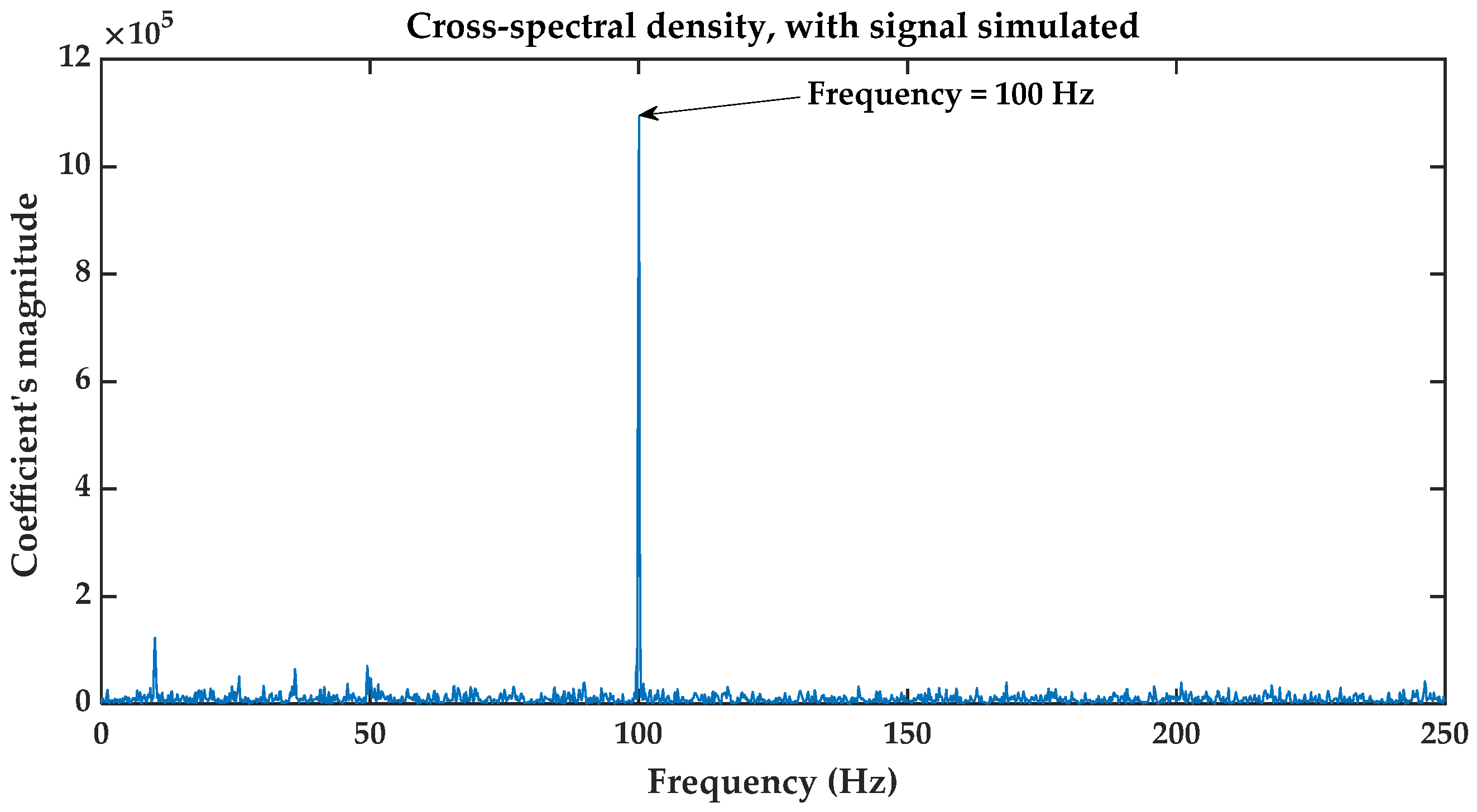
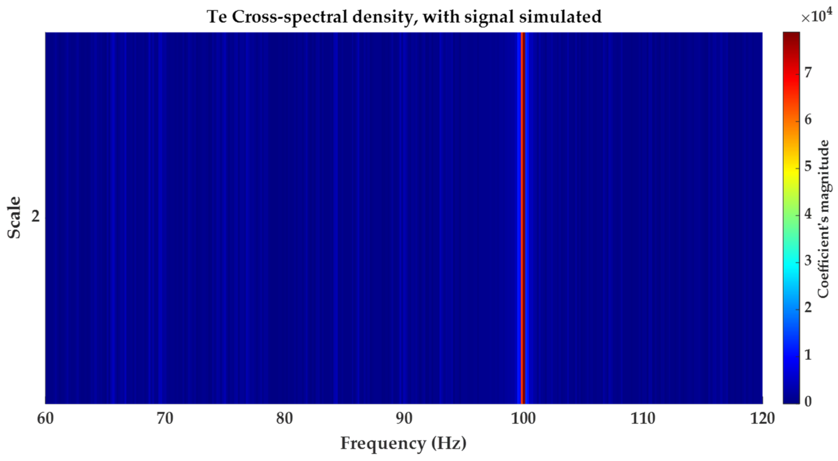
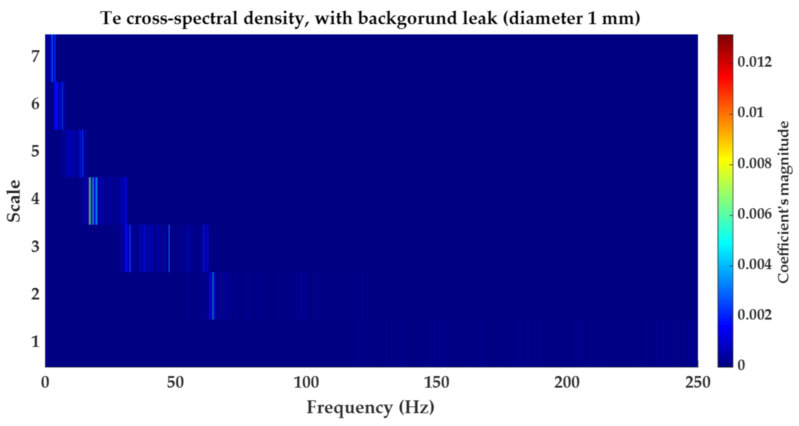
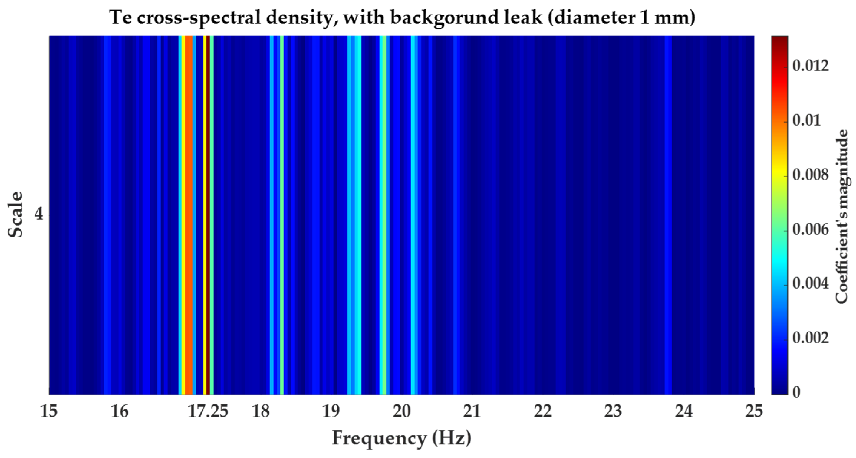
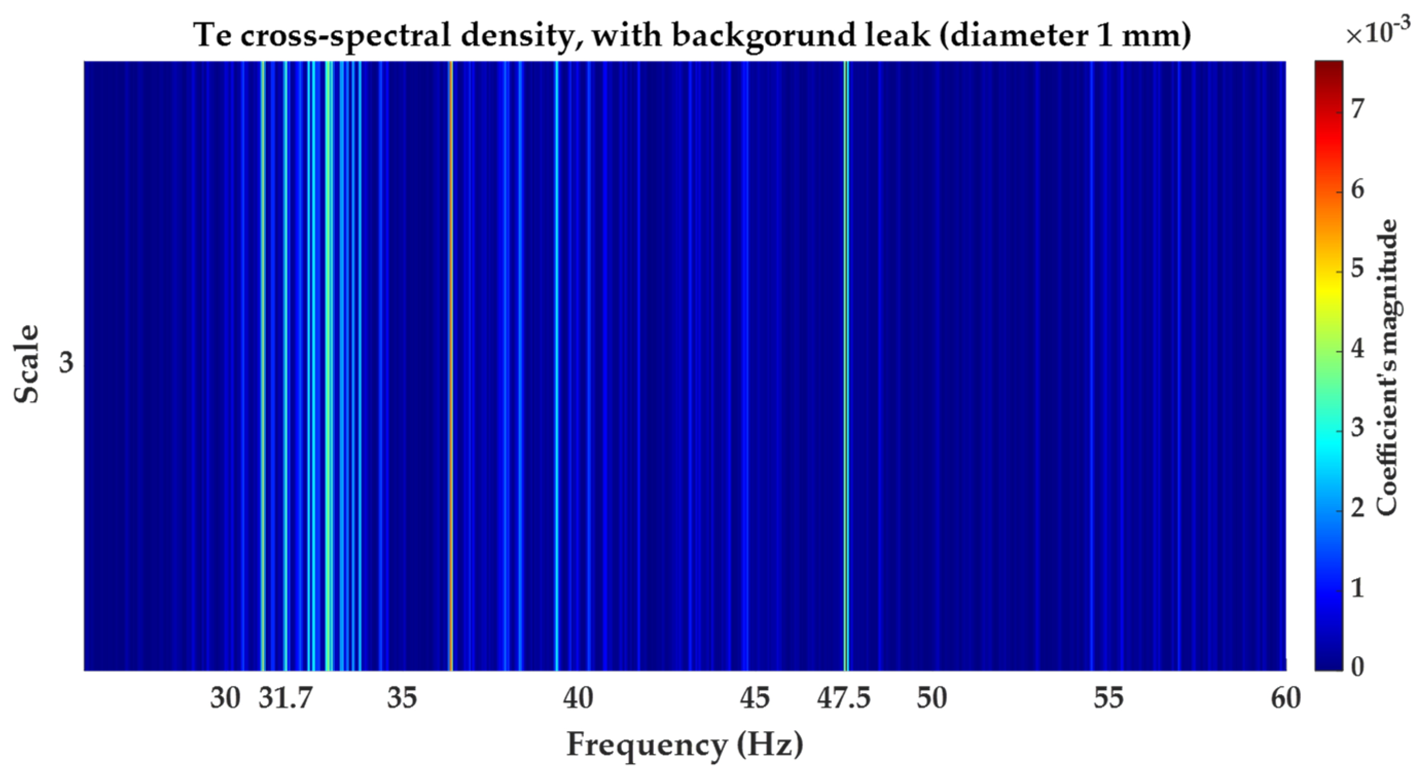
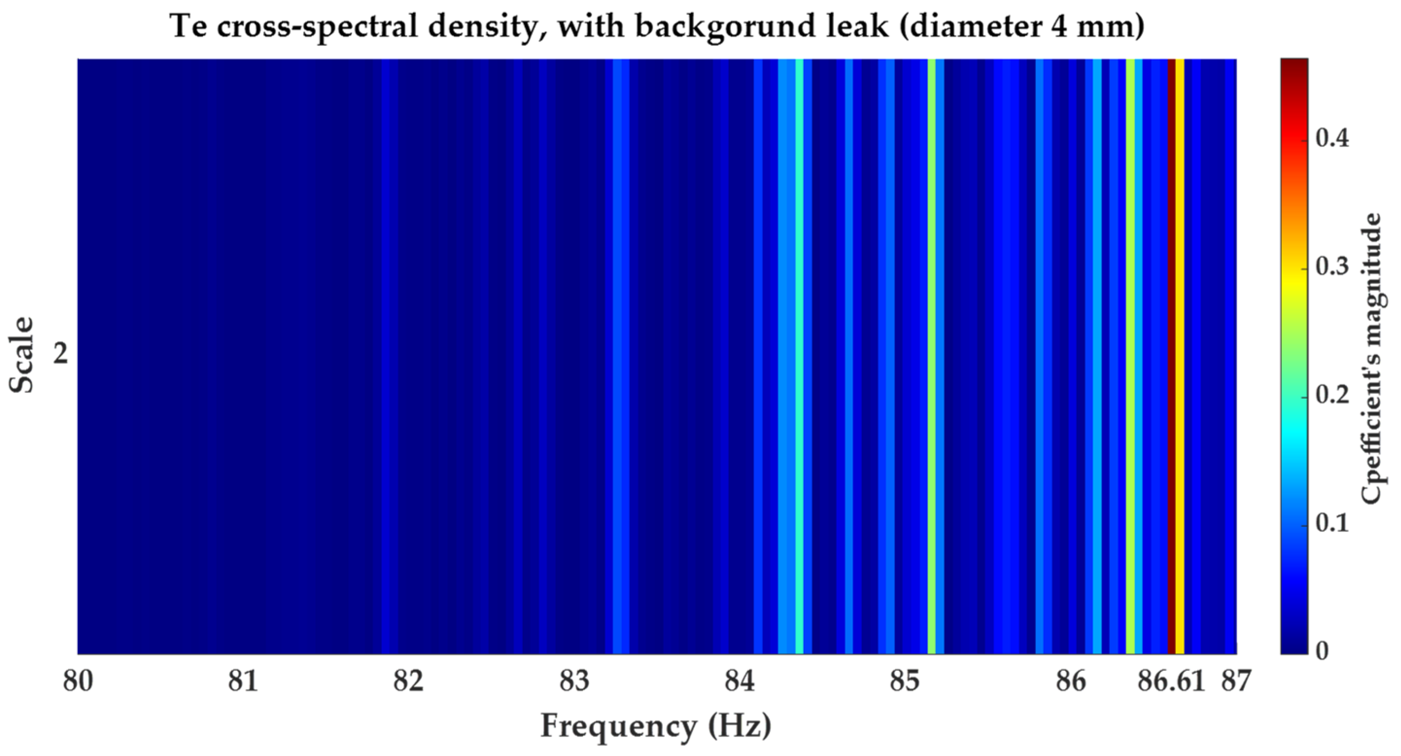
- The first is the cross-spectral density.
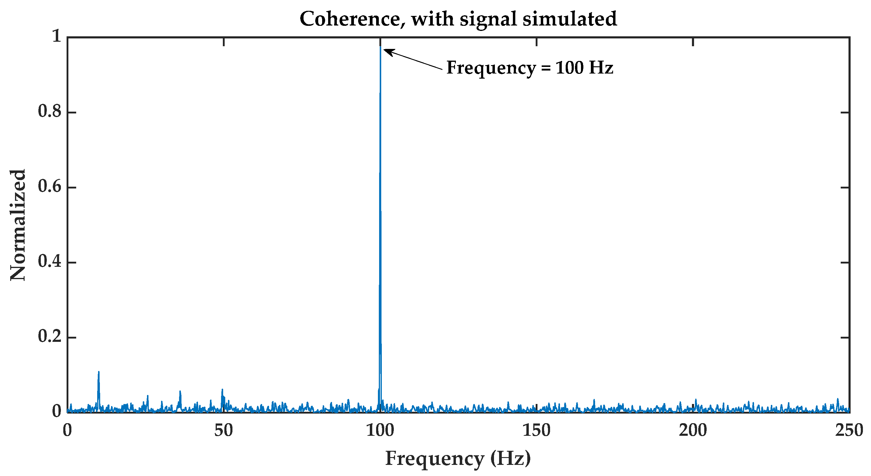
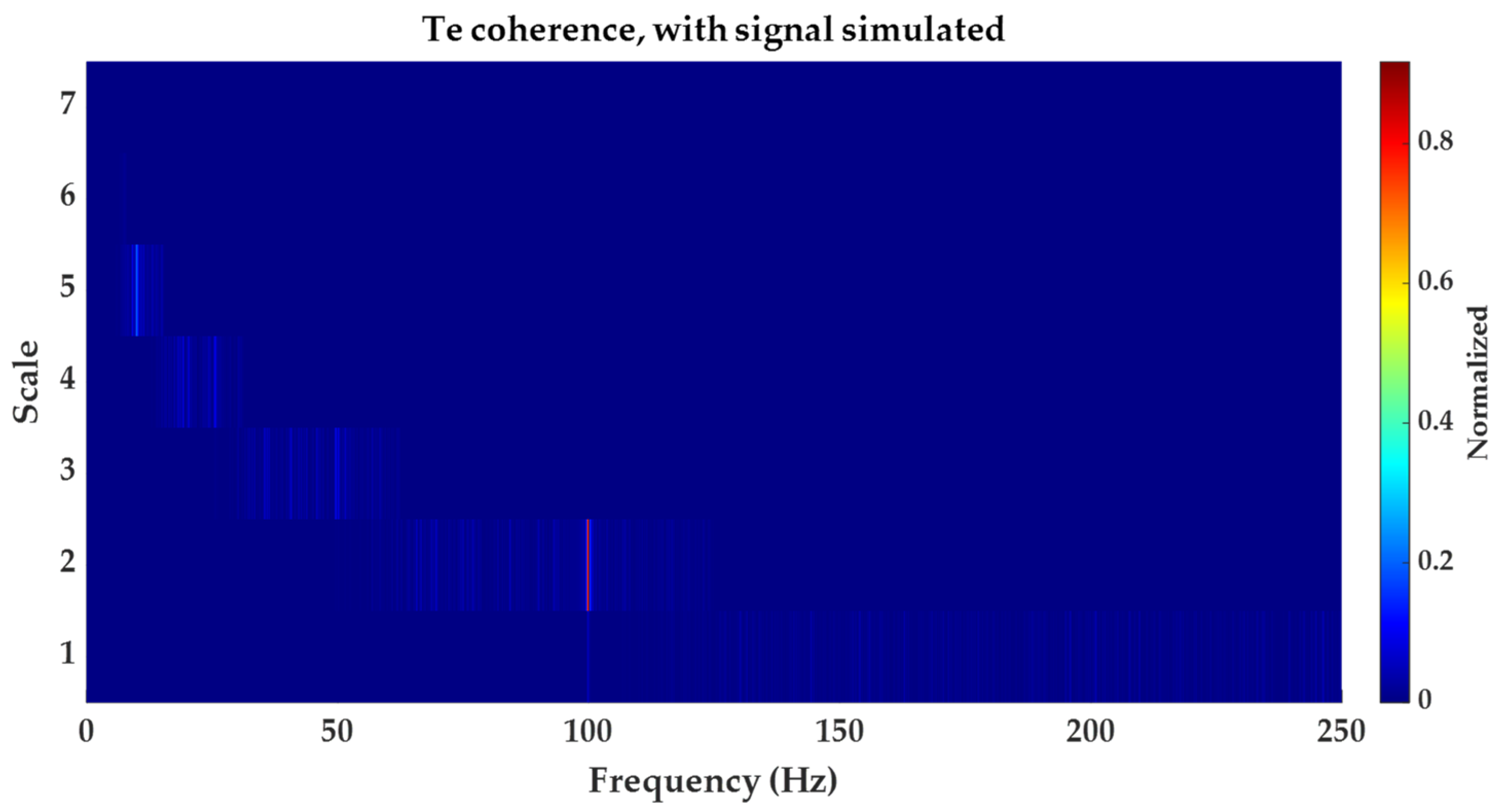
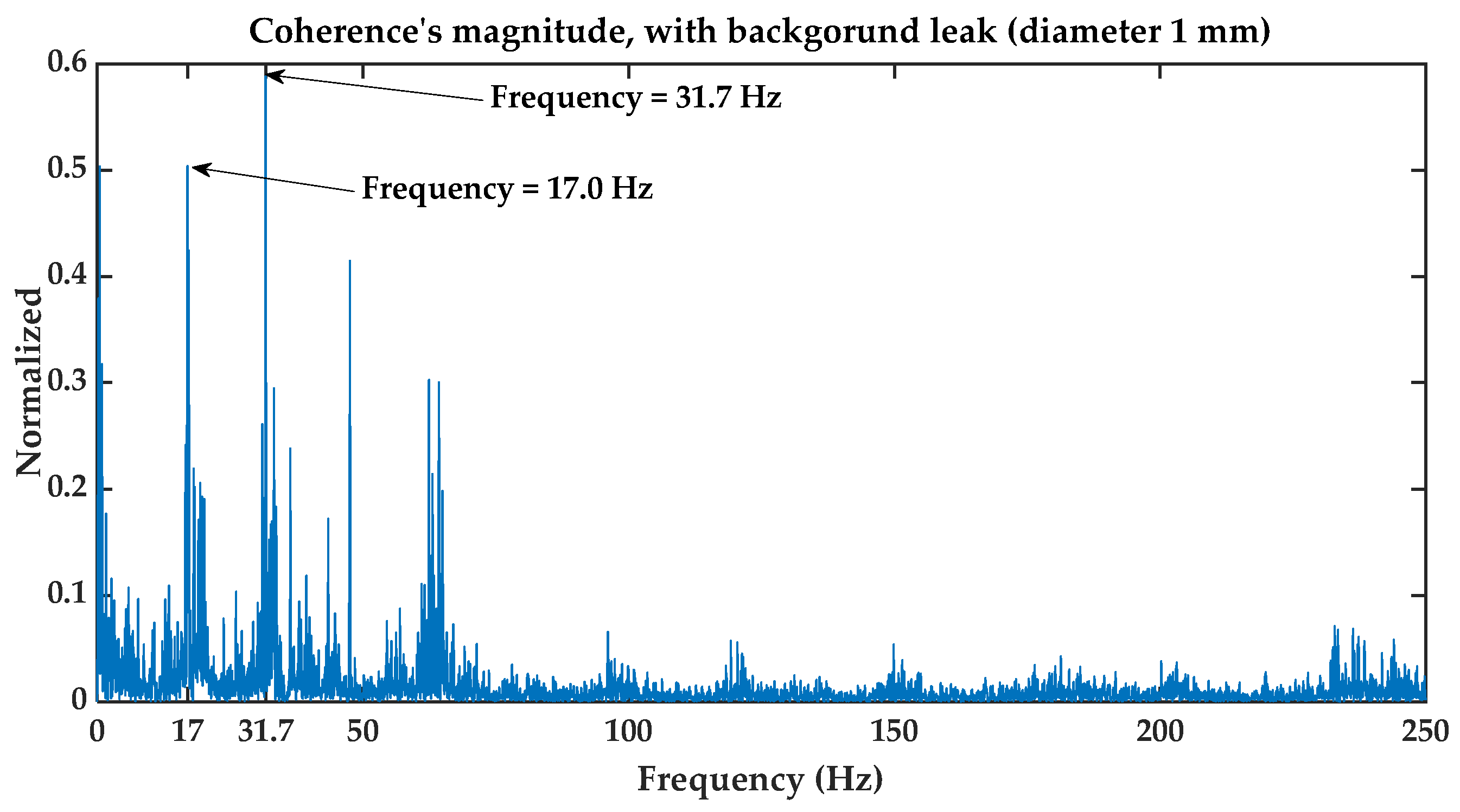
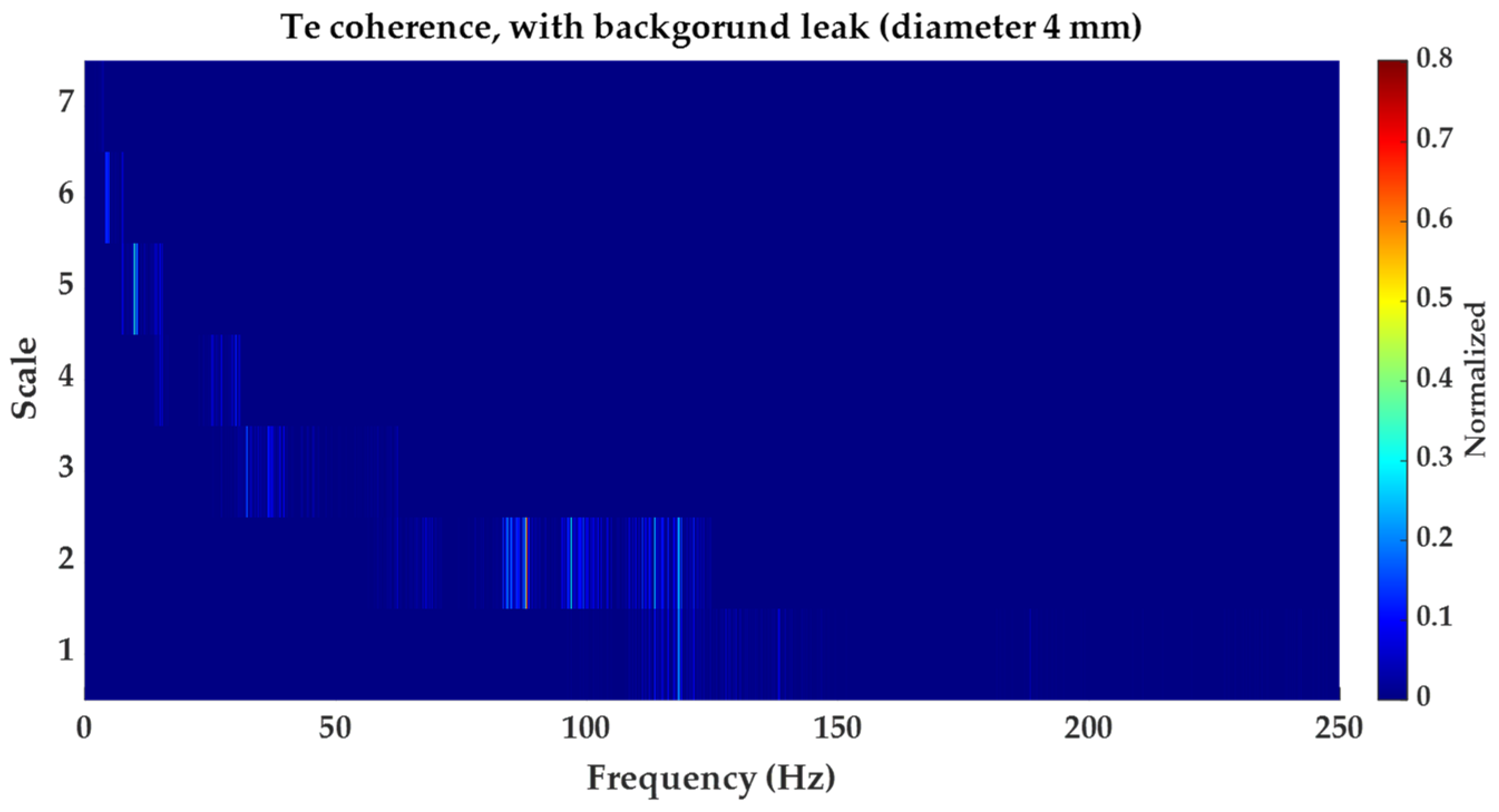
- The second is coherence.
2. Theoretical Background
2.1. Cross-Correlation Function
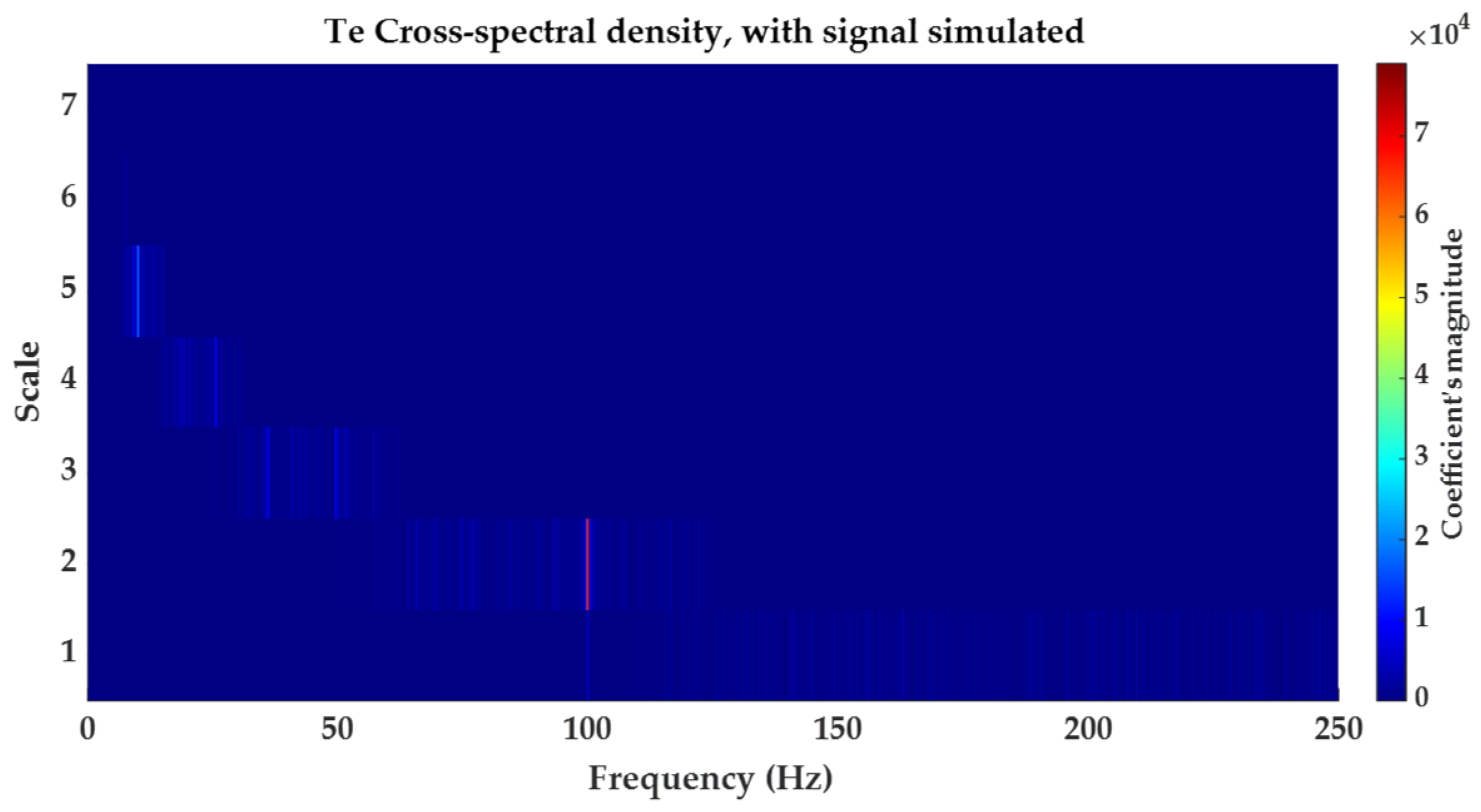
2.2. Transform
2.3. Cross-Spectral Density Function
2.4. Coherence Function
3. Method for the Detection of Water Background Leakage
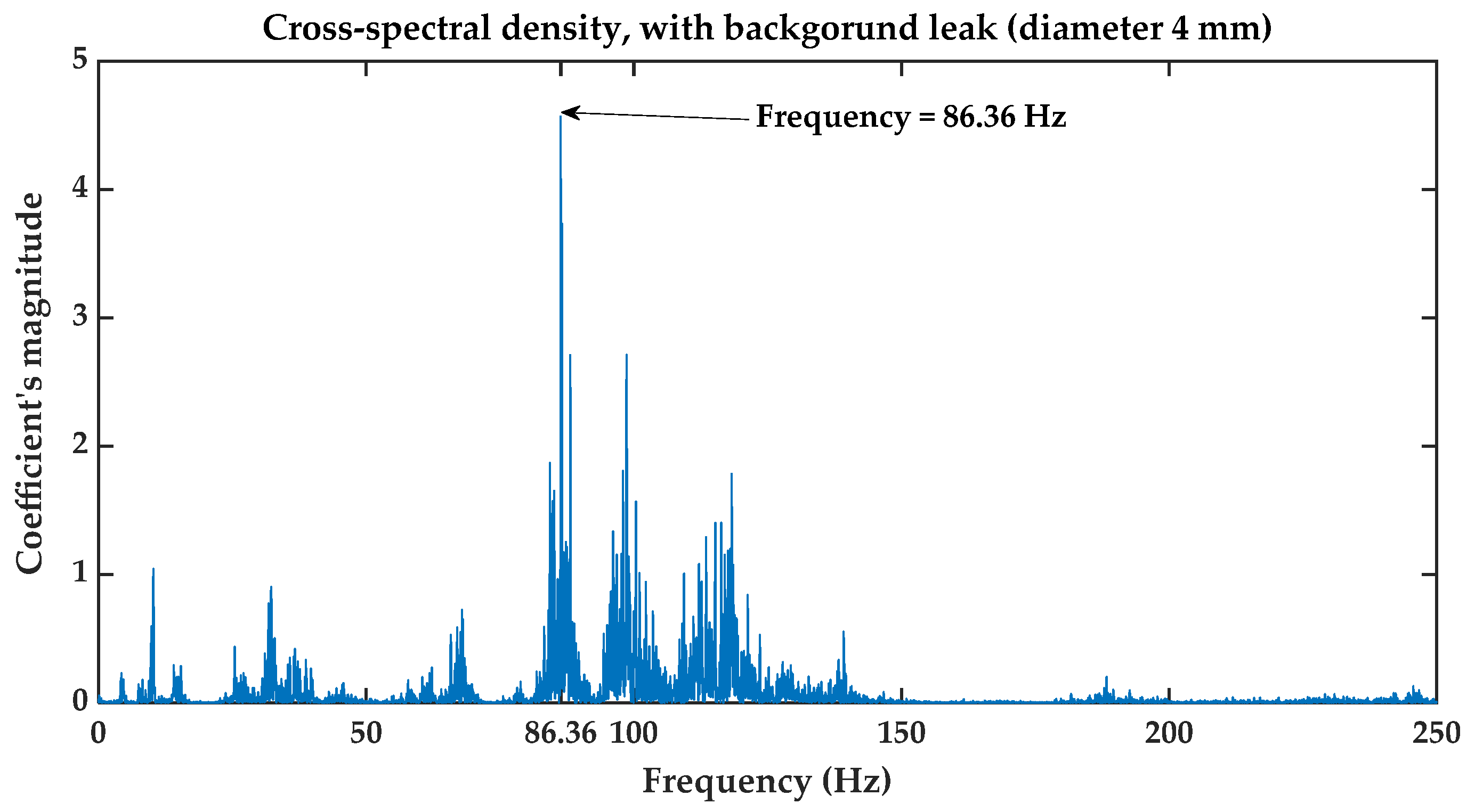
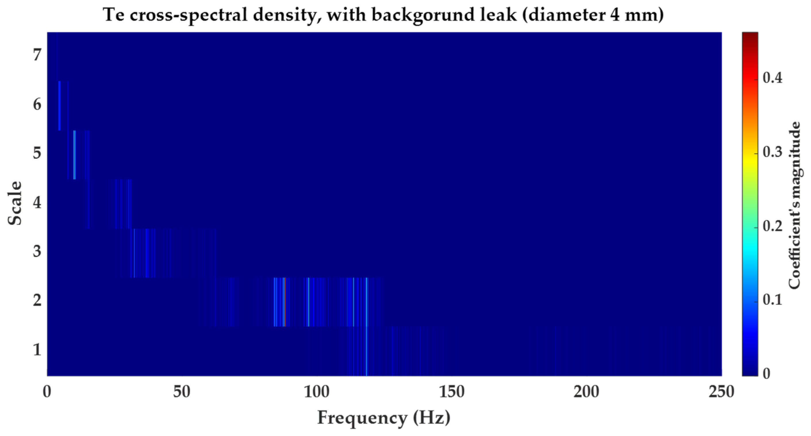
3.1. Cross-Spectral Density Function
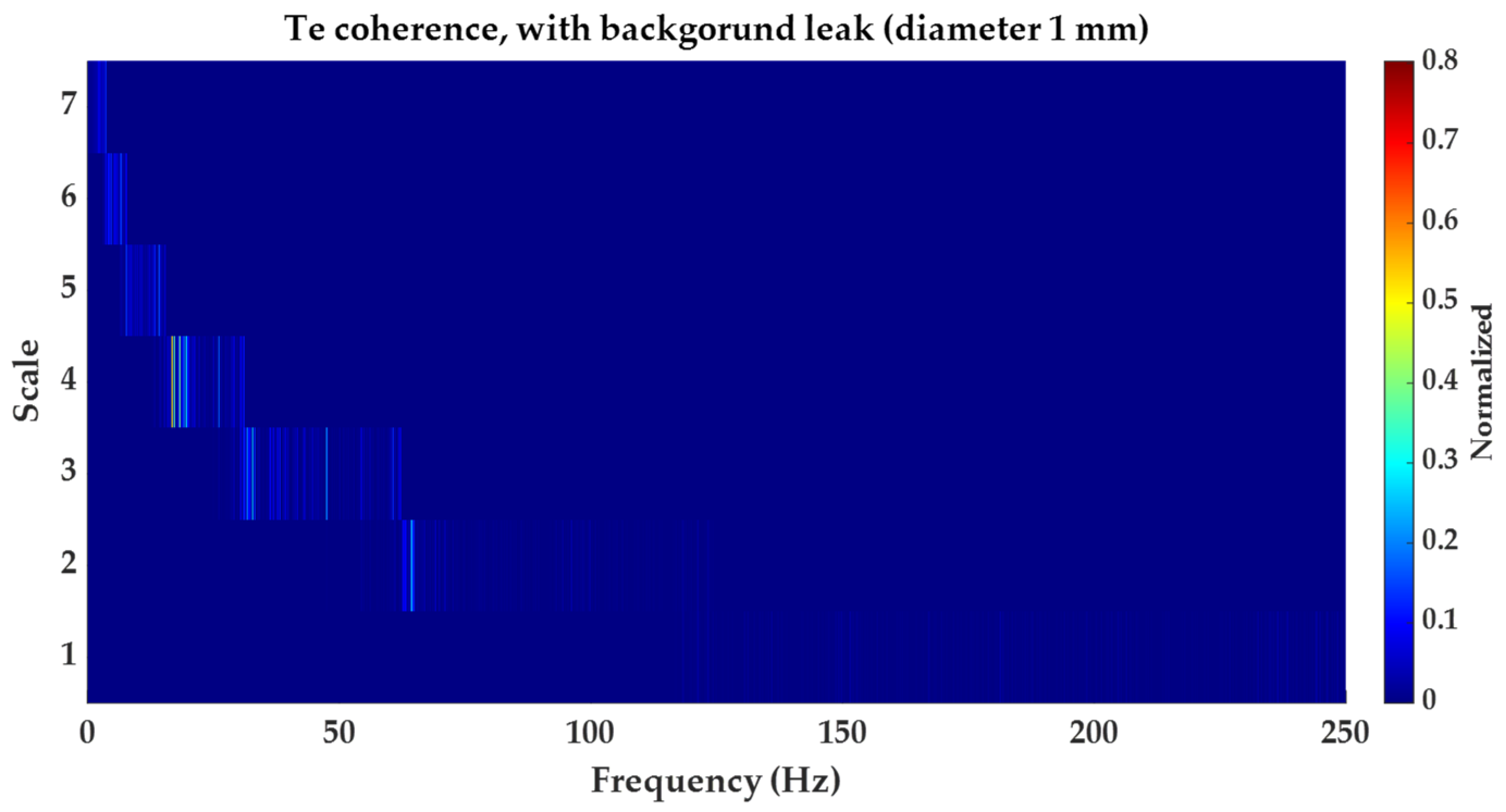
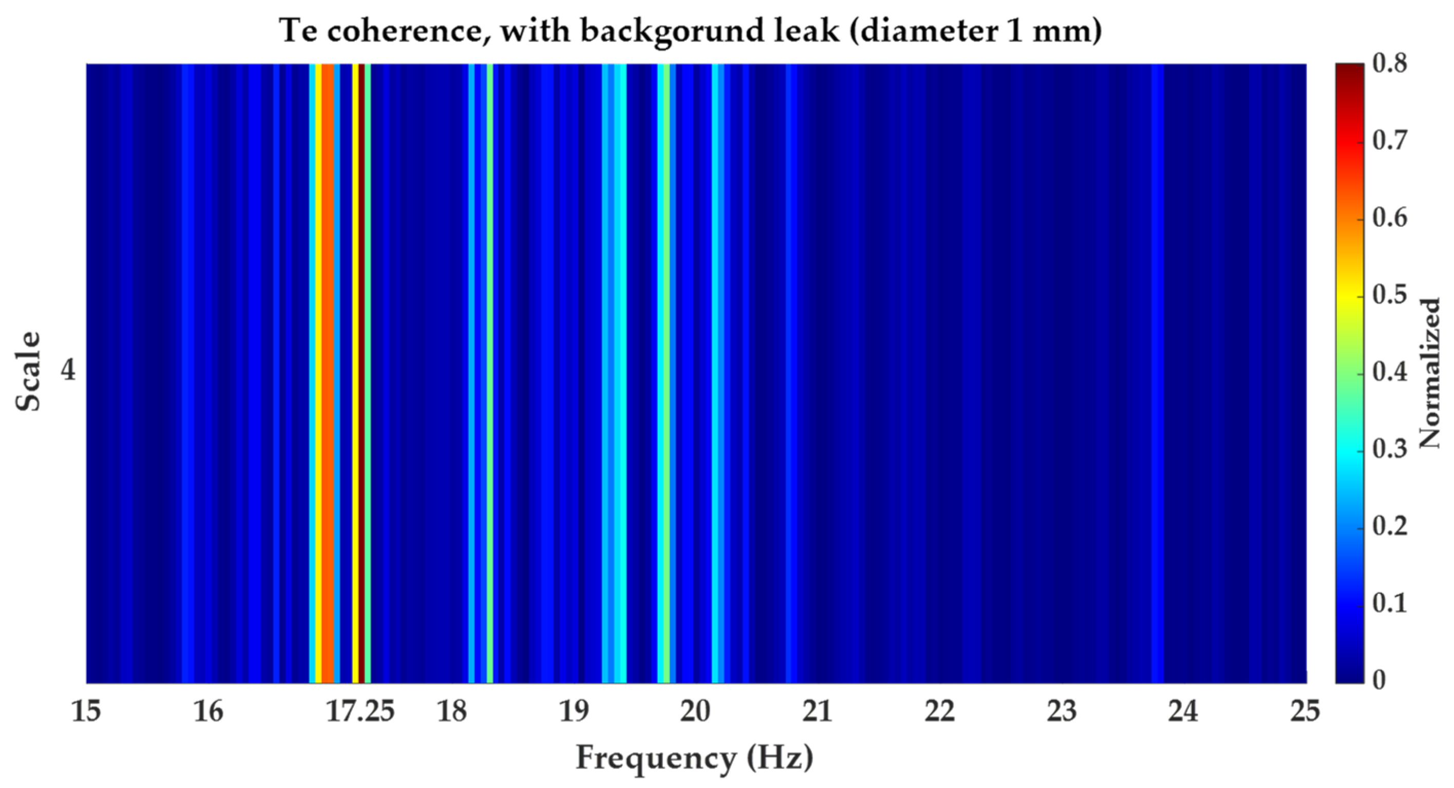
3.2. Coherence Function
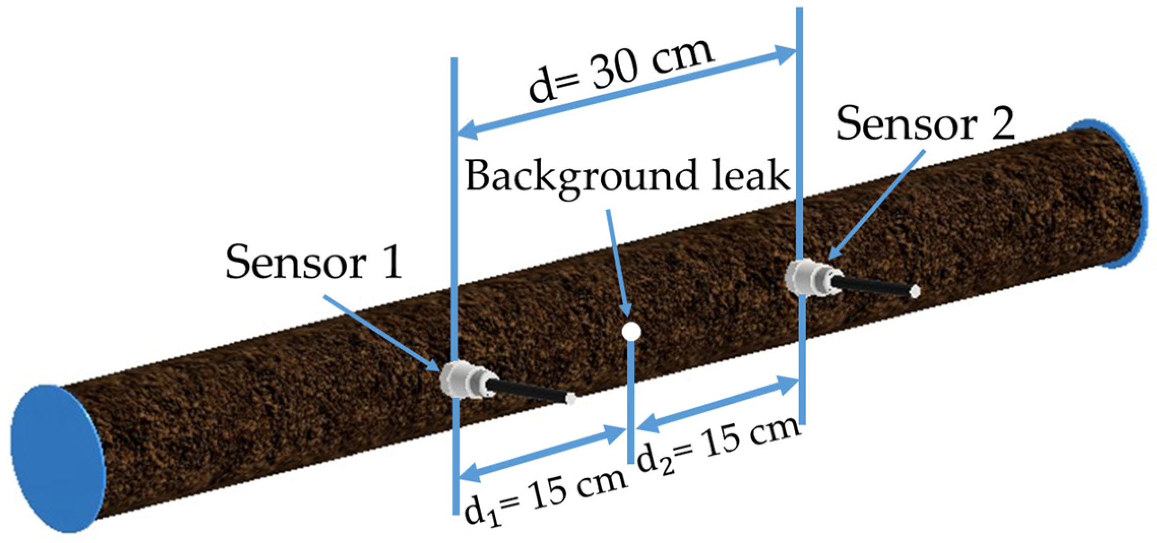
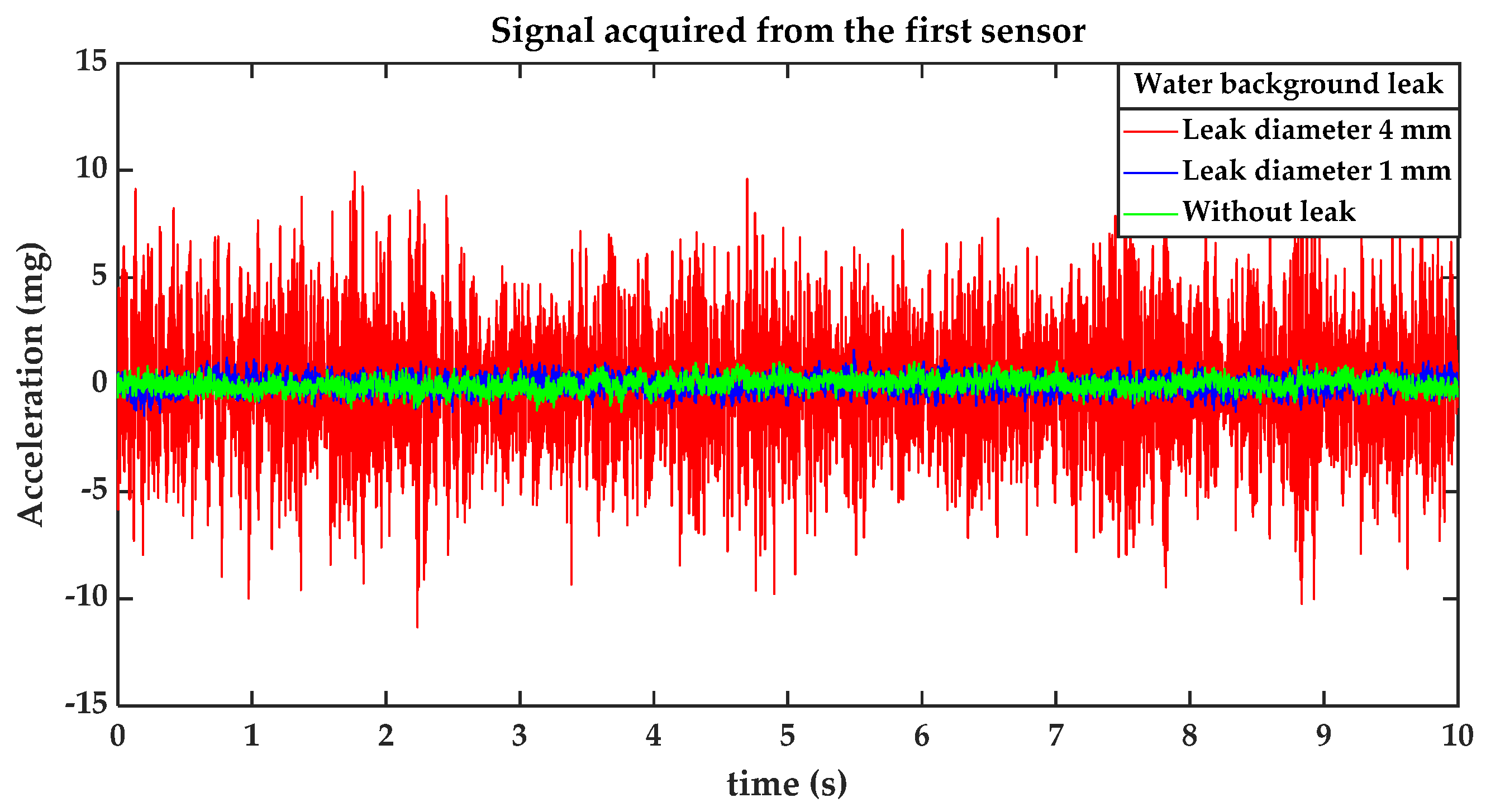
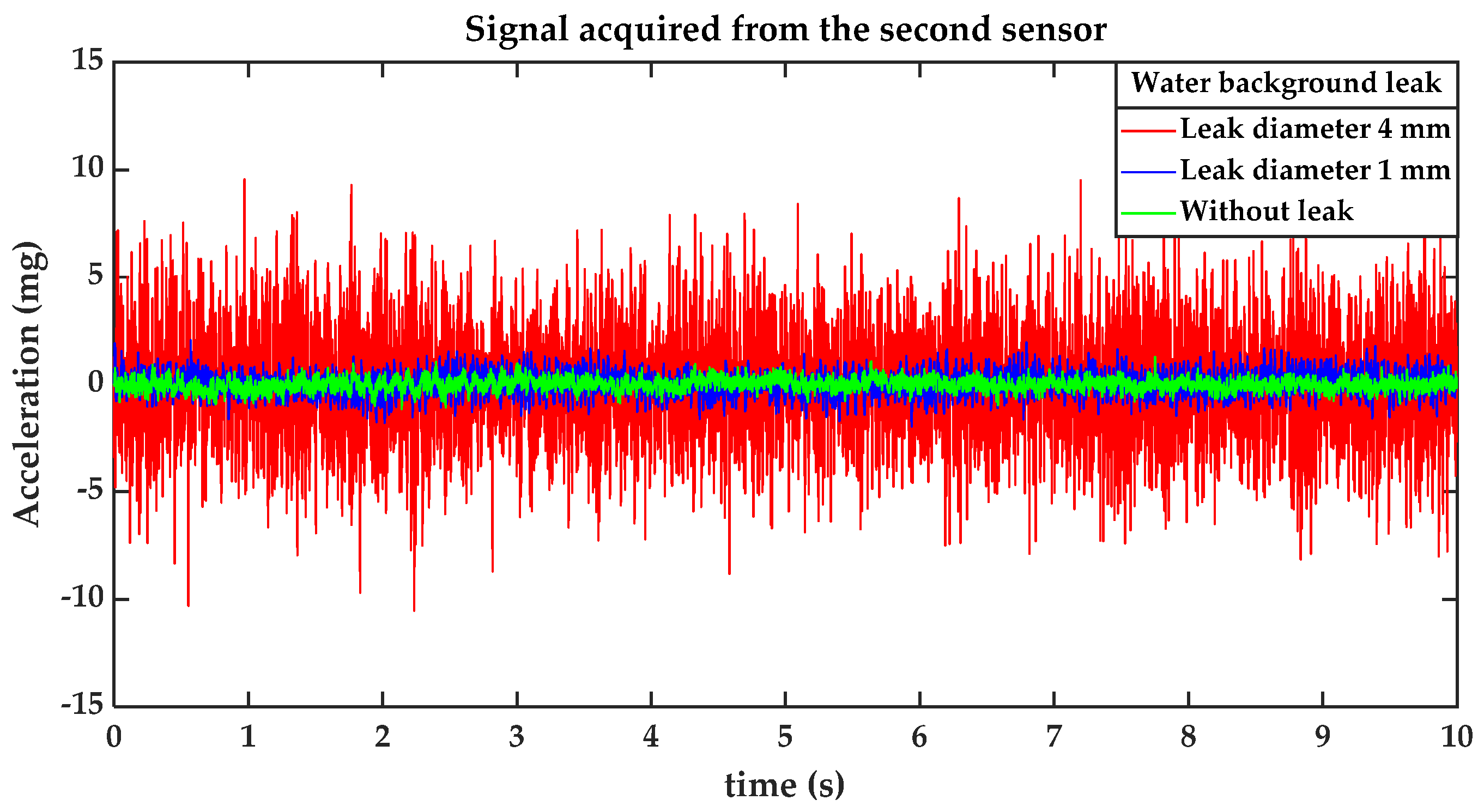
4. Experimental Design
5. Results and Discussion
5.1. Simulated Signal Scenario
5.2. Real Experimentation Scenarios
5.2.1. Results Obtained for Background Leakage of in Diameter
5.2.2. Results Obtained for Background Leakage of in Diameter
6. Conclusions
Author Contributions
Funding
Data Availability Statement
Acknowledgments
Conflicts of Interest
References
- Trutié-Carrero, E.; Seuret-Jimenez, D.; Nieto-Jalil, J.M. A high-resolution dyadic transform for non-stationary signal analysis. Mathematics 2021, 9, 3041. [Google Scholar] [CrossRef]
- Bang, S.S.; Lee, Y.H.; Shin, Y.J. Defect detection in pipelines via guided wave-based time-frequency-domain reflectometry. IEEE Trans. Instrum. Meas. 2021, 70, 9505811. [Google Scholar] [CrossRef]
- Keramat, A.; Karney, B.; Ghidaoui, M.S.; Wang, X. Transient-based leak detection in the frequency domain considering fluid–structure interaction and viscoelasticity. Mech. Syst. Signal Process. 2021, 153, 107500. [Google Scholar] [CrossRef]
- Wang, W.; Sun, H.; Guo, J.; Lao, L.; Wu, S.; Zhang, J. Experimental study on water pipeline leak using In-Pipe acoustic signal analysis and artificial neural network prediction. Meas. J. Int. Meas. Confed. 2021, 186, 110094. [Google Scholar] [CrossRef]
- Guo, C.; Shi, K.; Chu, X. Cross-correlation analysis of multiple fibre optic hydrophones for water pipeline leakage detection. Int. J. Environ. Sci. Technol. 2022, 19, 197–208. [Google Scholar] [CrossRef]
- Kothandaraman, M.; Law, Z.; Ezra, M.A.G.; Pua, C.; Rajasekaran, U. Water Pipeline Leak Measurement Using Wavelet Packet-based Adaptive ICA. Water Resour. Manag. 2022, 36, 1973–1989. [Google Scholar] [CrossRef]
- Jiang, W.; Du, L.; Luo, Z.; Wang, Z.; Song, H. Impact localization with a weighted spectral cross correlation method. Aerosp. Sci. Technol. 2022, 126, 107591. [Google Scholar] [CrossRef]
- Trutié-Carrero, E.; Valdés-Santiago, D.; León-Mećias, Á.; Ra, J. Burst detection and localization using discrete wavelet transform and cross-correlation. RIAI—Rev. Iberoam. Autom. e Inform. Ind. 2018, 15, 211–216. [Google Scholar] [CrossRef]
- Martini, A.; Troncossi, M.; Rivola, A. Vibration Monitoring as a Tool for Leak Detection in Water Distribution Networks. In: Ciri Din. 2014, p. 1. Available online: http://www.scopus.com/inward/record.url?eid=2-s2.0-84937219271&partnerID=tZOtx3y1 (accessed on 1 January 2023).
- Trutié-Carrero, E.; Cabrera-Hernández, Y.; Hernández-González, A.; Ramírez-Beltrán, J. Automatic detection of burst in water distribution systems by Lipschitz exponent and Wavelet correlation criterion. Meas. J. Int. Meas. Confed. 2020, 151, 107195. [Google Scholar] [CrossRef]
- Rathnayaka, S.; Shannon, B.; Rajeev, P.; Kodikara, J. Monitoring of pressure transients in water supply networks. Water Resour. Manag. 2015, 30, 471–485. [Google Scholar] [CrossRef]
- Ravisangar, V.; Charles, T. Special considerations for protecting very long transmission mains from hydraulic transients. In Pipelines 2011 A Sound Conduit for Sharing Solutions; ASCE: Reston, VA, USA, 2011; pp. 1215–1224. [Google Scholar] [CrossRef]
- Kumar, D.; Tu, D.; Zhu, N.; Shah, R.A.; Hou, D.; Zhang, H. The free-swimming device leakage detection in plastic water-filled pipes through tuning the wavelet transform to the underwater acoustic signals. Water 2017, 9, 731. [Google Scholar] [CrossRef]
- Ayala, P.; Brennan, M.; Almeida, F.; Kroll, F.; Obata, D.; Tabone, A. Vibroacoustic characteristics of leak noise in buried water pipes in Brazil. In Proceedings of the I Jornada Peruana Internacional de Investigación en Ingeniería, Lima, Peru, 11–13 January 2017. [Google Scholar]
- Butterfield, J.D.; Krynkin, A.; Collins, R.P.; Beck, S.B.M. Experimental investigation into vibro-acoustic emission signal processing techniques to quantify leak flow rate in plastic water distribution pipes. Appl. Acoust. 2017, 119, 146–155. [Google Scholar] [CrossRef]
- Butterfield, J.D.; Collins, R.P.; Beck, S.B.M. Influence of Pipe Material on the Transmission of Vibroacoustic Leak Signals in Real Complex Water Distribution Systems: Case Study. J. Pipeline Syst. Eng. Pract. 2018, 9, 05018003. [Google Scholar] [CrossRef]
- Gao, Y.; Liu, Y.; Ma, Y.; Cheng, X.; Yang, J. Application of the differentiation process into the correlation-based leak detection in urban pipeline networks. Mech. Syst. Signal Process. 2018, 112, 251–264. [Google Scholar] [CrossRef]
- Trutié-Carrero, E.; Delgado-Hernández, L.A.; González-Zamora, C.; Ramírez-Beltrán, J. Detección y localización de fuga de fondo en tuberías plásticas de agua bajo un ambiente ruidoso. Rev. Ing. Electrón. Autom. Comun. 2019, 40, 1–15. [Google Scholar]
- Kassab, S.; Michel, F.; Maxit, L. Water experiment for assessing vibroacoustic beamforming gain for acoustic leak detection in a sodium-heated steam generator. Mech. Syst. Signal Process. 2019, 134, 106332. [Google Scholar] [CrossRef]
- Xue, Z.; Tao, L.; Fuchun, J.; Riehle, E.; Xiang, H.; Bowen, N.; Prasad, R. Application of acoustic intelligent leak detection in an urban water supply pipe network. J. Water Supply Res. Technol.—AQUA 2020, 69, 512–520. [Google Scholar] [CrossRef]
- Cody, R.A.; Dey, P.; Narasimhan, S. Linear Prediction for Leak Detection in Water Distribution Networks. J. Pipeline Syst. Eng. Pract. 2020, 11, 04019043. [Google Scholar] [CrossRef]
- Gao, L.; Li, D.; Yao, L.; Gao, Y. Sensor drift fault diagnosis for chiller system using deep recurrent canonical correlation analysis and k-nearest neighbor classifier. ISA Trans. 2022, 122, 232–246. [Google Scholar] [CrossRef]
- Liu, Z.; Fang, L.; Jiang, D.; Qu, R. A Machine-Learning-Based Fault Diagnosis Method With Adaptive Secondary Sampling for Multiphase Drive Systems. IEEE Trans. Power Electron. 2022, 37, 8767–8772. [Google Scholar] [CrossRef]
- Chen, B.; Cheng, Y.; Zhang, W.; Mei, G. Investigation on enhanced mathematical morphological operators for bearing fault feature extraction. ISA Trans. 2022, 126, 440–459. [Google Scholar] [CrossRef] [PubMed]
- Oppenheim, A.V.; Schafer, R.W. Digital Signal Processing; Research supported by the Massachusetts Institute of Technology, Bell Telephone Laboratories, and Guggenheim Foundation, Englewood Cliffs, N.J.; Prentice-Hall, Inc.: Hoboken, NJ, USA, 1975; p. 598. [Google Scholar]
- Gao, Y.; Brennan, M.J.; Joseph, P.F. On the effects of reflections on time delay estimation for leak detection in buried plastic water pipes. J. Sound Vib. 2009, 325, 649–663. [Google Scholar] [CrossRef]
- Li, S.; Cai, M.; Han, M.; Dai, Z. Noise Reduction Based on CEEMDAN-ICA and Cross-Spectral Analysis for Leak Location in Water-supply Pipelines. IEEE Sens. J. 2022, 22, 13030–13042. [Google Scholar] [CrossRef]
- Wen, H.; Zhang, L.; Sinha, J. Adaptive Band Extraction Based on Low Rank Approximated Nonnegative Tucker Decomposition for Anti-Friction Bearing Faults Diagnosis Using Measured Vibration Data. Machines 2022, 10, 694. [Google Scholar] [CrossRef]
- Wang, Z.; Yang, J.; Li, H.; Zhen, D.; Gu, F.; Ball, A. Improved cyclostationary analysis method based on TKEO and its application on the faults diagnosis of induction motors. ISA Trans. 2022, 128, 513–530. [Google Scholar] [CrossRef]
- Medina, R.; Garrido, M. Improving impact-echo method by using cross-spectral density. J. Sound Vib. 2007, 304, 769–778. [Google Scholar] [CrossRef]
- Manolakis, D.G.; Ingle, V.K.; Kogon, S.M. Spectral Estimation, Signal Modeling, Adaptive Filtering, and Array Processing; ARTECH HOUSE: Boston, MA, USA, 2005. [Google Scholar]
- Chen, B.; Cheng, Y.; Zhang, W.; Gu, F. Enhanced bearing fault diagnosis using integral envelope spectrum from spectral coherence normalized with feature energy. Meas. J. Int. Meas. Confed. 2022, 189, 110448. [Google Scholar] [CrossRef]
- Zhang, B.; Miao, Y.; Lin, J.; Li, H. Weighted envelope spectrum based on the spectral coherence for bearing diagnosis. ISA Trans. 2022, 123, 398–412. [Google Scholar] [CrossRef]
- Allemang, R.J.; Patwardhan, R.S.; Kolluri, M.M.; Phillips, A.W. Frequency response function estimation techniques and the corresponding coherence functions: A review and update. Mech. Syst. Signal Process. 2022, 162, 108100. [Google Scholar] [CrossRef]
- Dragos, K.; Magalhães, F.; Manolis, G.D.; Smarsly, K. Cross-Spectrum-Based Synchronization of Structural Health Monitoring Data. In European Workshop on Structural Health Monitoring: EWSHM 2022-Volume 2; Springer: Cham, Switzerland, 2023; pp. 927–936. [Google Scholar] [CrossRef]
- Kyophilavong, P.; Abakah, E.J.A.; Tiwari, A.K. Cross-spectral coherence and co-movement between WTI oil price and exchange rate of Thai Baht. Resour. Policy 2023, 80, 103160. [Google Scholar] [CrossRef]
- Bo, T.L.; Li, F. Multi-scale characteristics of the spatial distribution of space charge density that determines the vertical electric field during dust storms. Granul. Matter. 2023, 25, 6. [Google Scholar] [CrossRef]
- Grinsted, A.; Moore, J.C.; Jevrejeva, S. Application of the cross wavelet transform and wavelet coherence to geophysical time series. Nonlinear Process. Geophys. 2004, 11, 561–566. [Google Scholar] [CrossRef]
- Olanrewaju, V.O.; Adebayo, T.S.; Akinsola, G.D.; Odugbesan, J.A. Determinants of Environmental Degradation in Thailand: Empirical Evidence from ARDL and Wavelet Coherence Approaches. Pollution 2021, 7, 181–196. [Google Scholar] [CrossRef]
- Mohammadzadeh, L.; Latifi, H.; Khaksar, S.; Feiz, M.S.; Motamedi, F.; Asadollahi, A.; Ezzatpour, M. Measuring the Frequency-Specific Functional Connectivity Using Wavelet Coherence Analysis in Stroke Rats Based on Intrinsic Signals. Sci. Rep. 2020, 10, 9429. [Google Scholar] [CrossRef] [PubMed]
- Gao, Z.; Lin, J.; Wang, X.; Liao, Y. Grinding Burn Detection Based on Cross Wavelet and Wavelet Coherence Analysis by Acoustic Emission Signal. Chin. J. Mech. Eng. 2019, 32, 68. [Google Scholar] [CrossRef]
- Carrera-Avendaño, E.; Urquiza-Beltrán, G.; Trutié-Carrero, E.; Nieto-Jalil, J.M.; Carrillo-Pereyra, C.; Seuret-Jiménez, D. Detection of crankshaft faults by means of a modified Welch-Bartlett periodogram. Eng. Fail. Anal. 2022, 132, 105938. [Google Scholar] [CrossRef]


Disclaimer/Publisher’s Note: The statements, opinions and data contained in all publications are solely those of the individual author(s) and contributor(s) and not of MDPI and/or the editor(s). MDPI and/or the editor(s) disclaim responsibility for any injury to people or property resulting from any ideas, methods, instructions or products referred to in the content. |
© 2023 by the authors. Licensee MDPI, Basel, Switzerland. This article is an open access article distributed under the terms and conditions of the Creative Commons Attribution (CC BY) license (https://creativecommons.org/licenses/by/4.0/).
Share and Cite
Trutié-Carrero, E.; Seuret-Jiménez, D.; Nieto-Jalil, J.M.; Herrera-Díaz, J.C.; Cantó, J.; Escobedo-Alatorre, J.J. Detection of Background Water Leaks Using a High-Resolution Dyadic Transform. Water 2023, 15, 736. https://doi.org/10.3390/w15040736
Trutié-Carrero E, Seuret-Jiménez D, Nieto-Jalil JM, Herrera-Díaz JC, Cantó J, Escobedo-Alatorre JJ. Detection of Background Water Leaks Using a High-Resolution Dyadic Transform. Water. 2023; 15(4):736. https://doi.org/10.3390/w15040736
Chicago/Turabian StyleTrutié-Carrero, Eduardo, Diego Seuret-Jiménez, José M. Nieto-Jalil, Julio C. Herrera-Díaz, Jorge Cantó, and J. Jesús Escobedo-Alatorre. 2023. "Detection of Background Water Leaks Using a High-Resolution Dyadic Transform" Water 15, no. 4: 736. https://doi.org/10.3390/w15040736