
Long-Term Trend and Variability of Volume Transport and Advective Heat Flux through the Boundaries of the Java Sea Based on a Global Ocean Circulation Model (1950–2013)
Abstract
:1. Introduction
2. Materials and Methods
2.1. Data
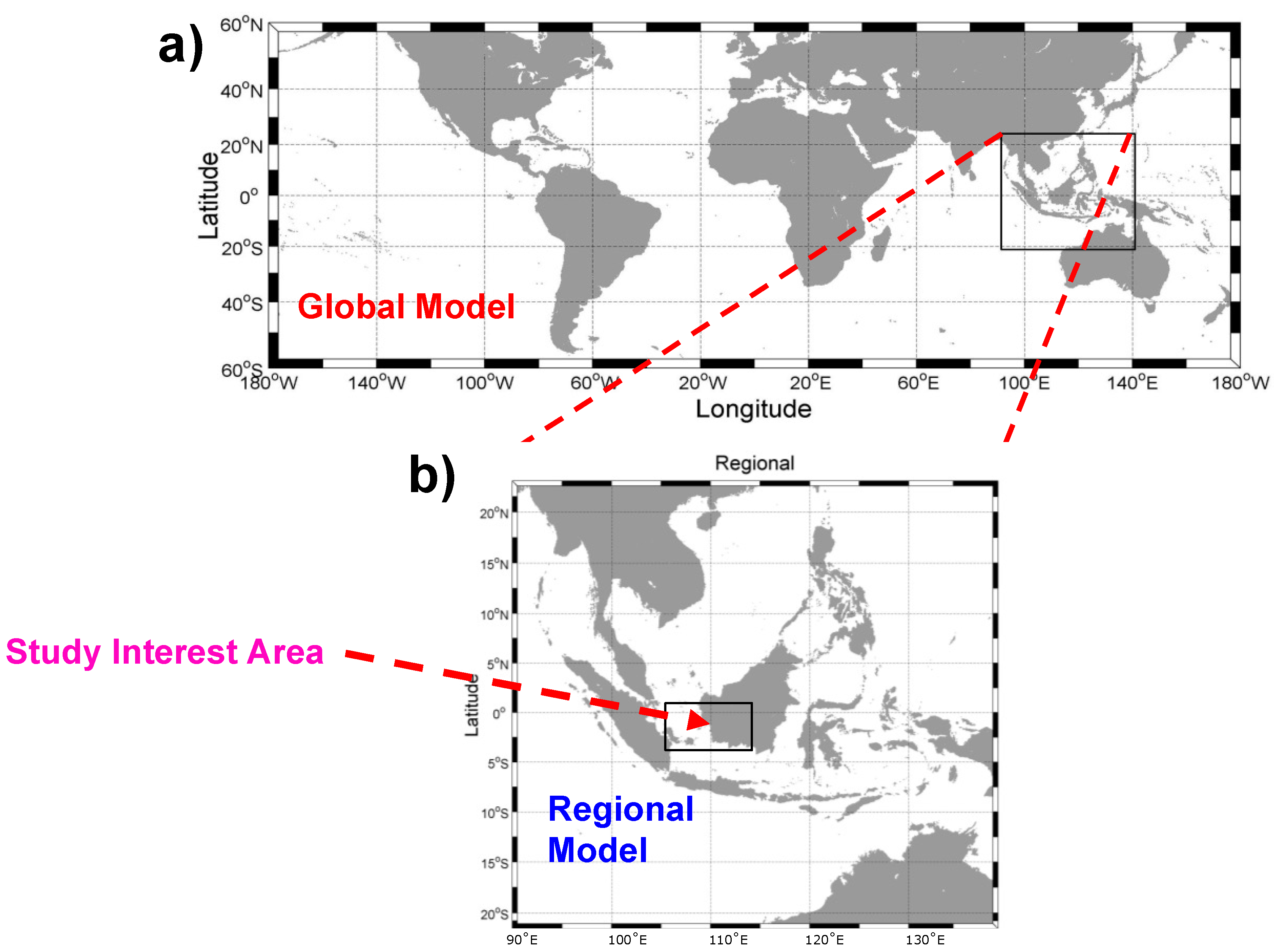
2.2. Model Setup Experiment
3. Results
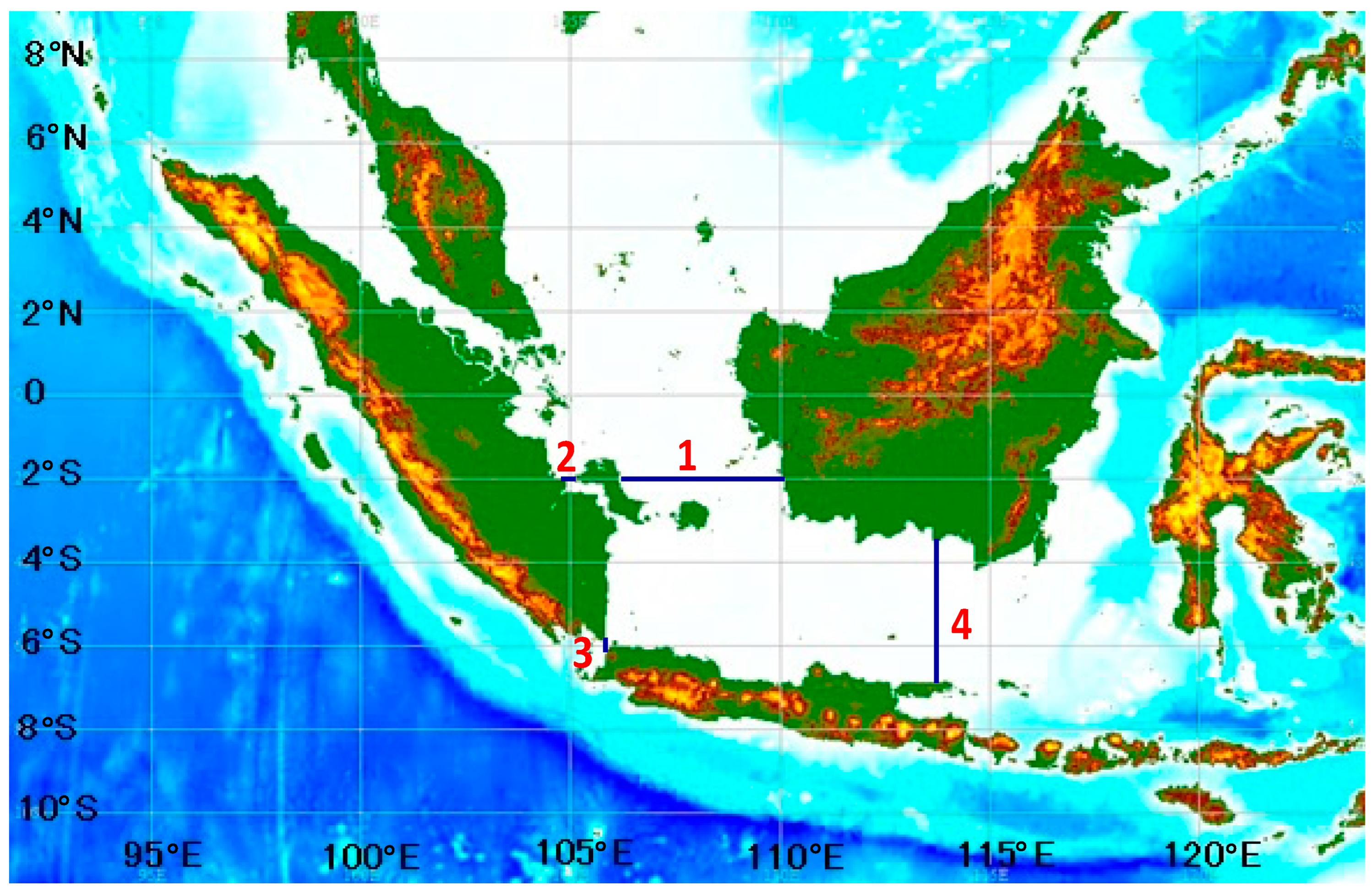
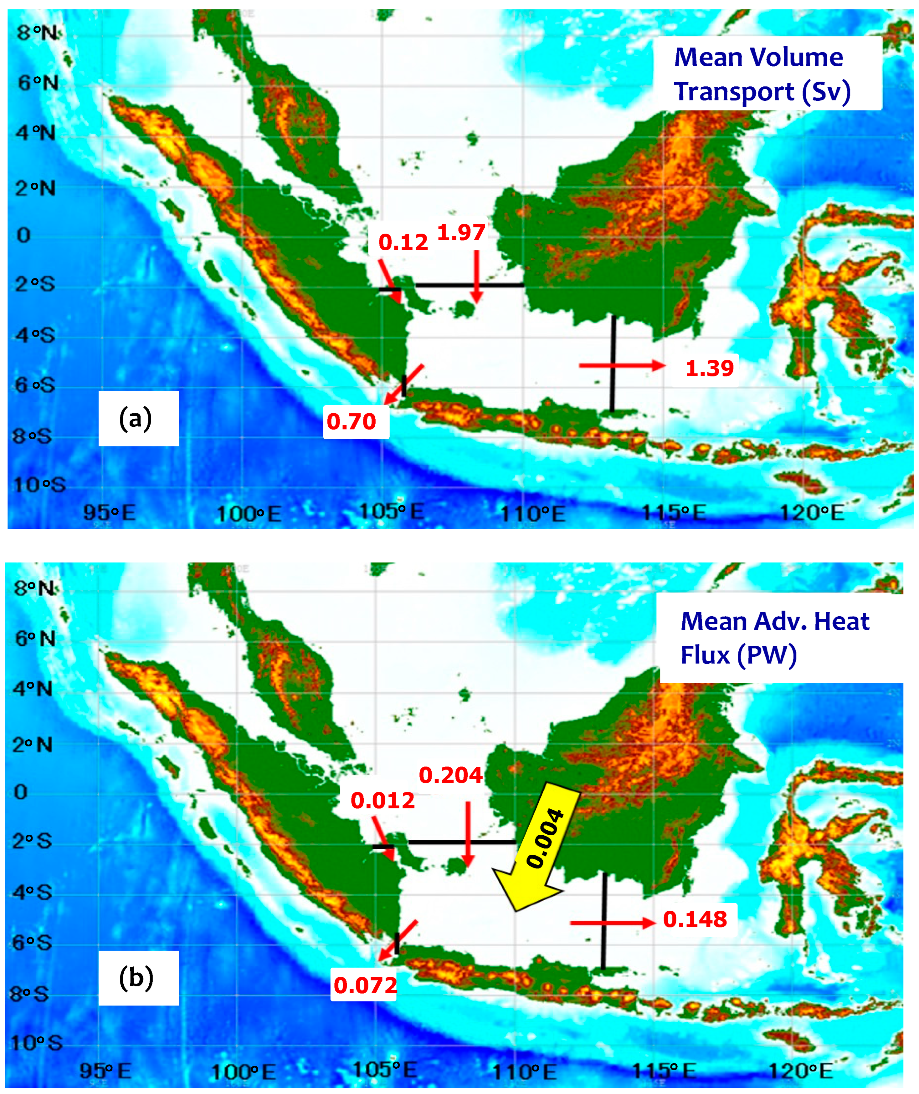
3.1. Zonal and Meridional Volume Transport and Advective Heat Flux through the Boundaries of the Java Sea
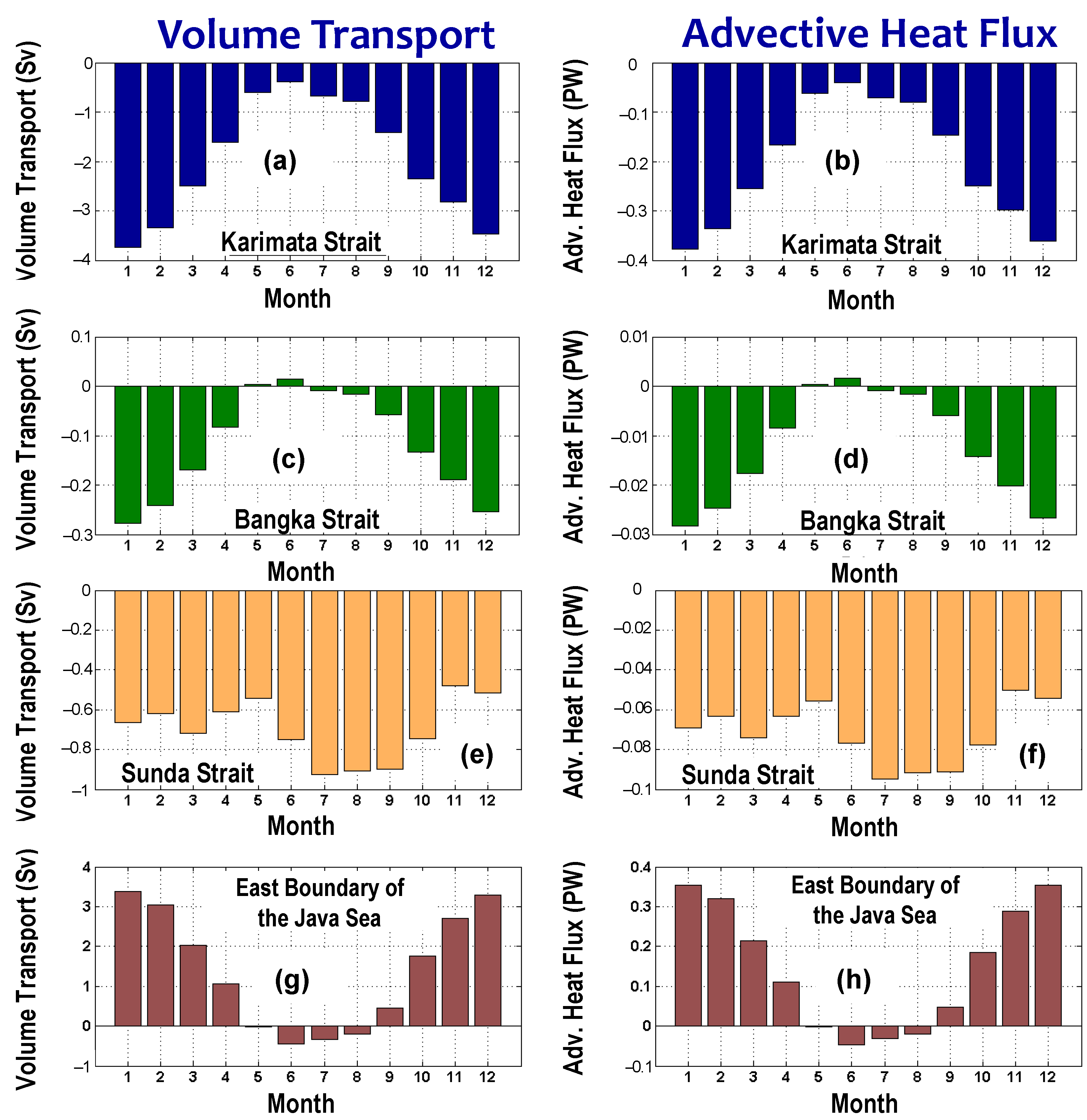
3.2. Seasonal Variations of Volume Transport and Advective Heat Flux
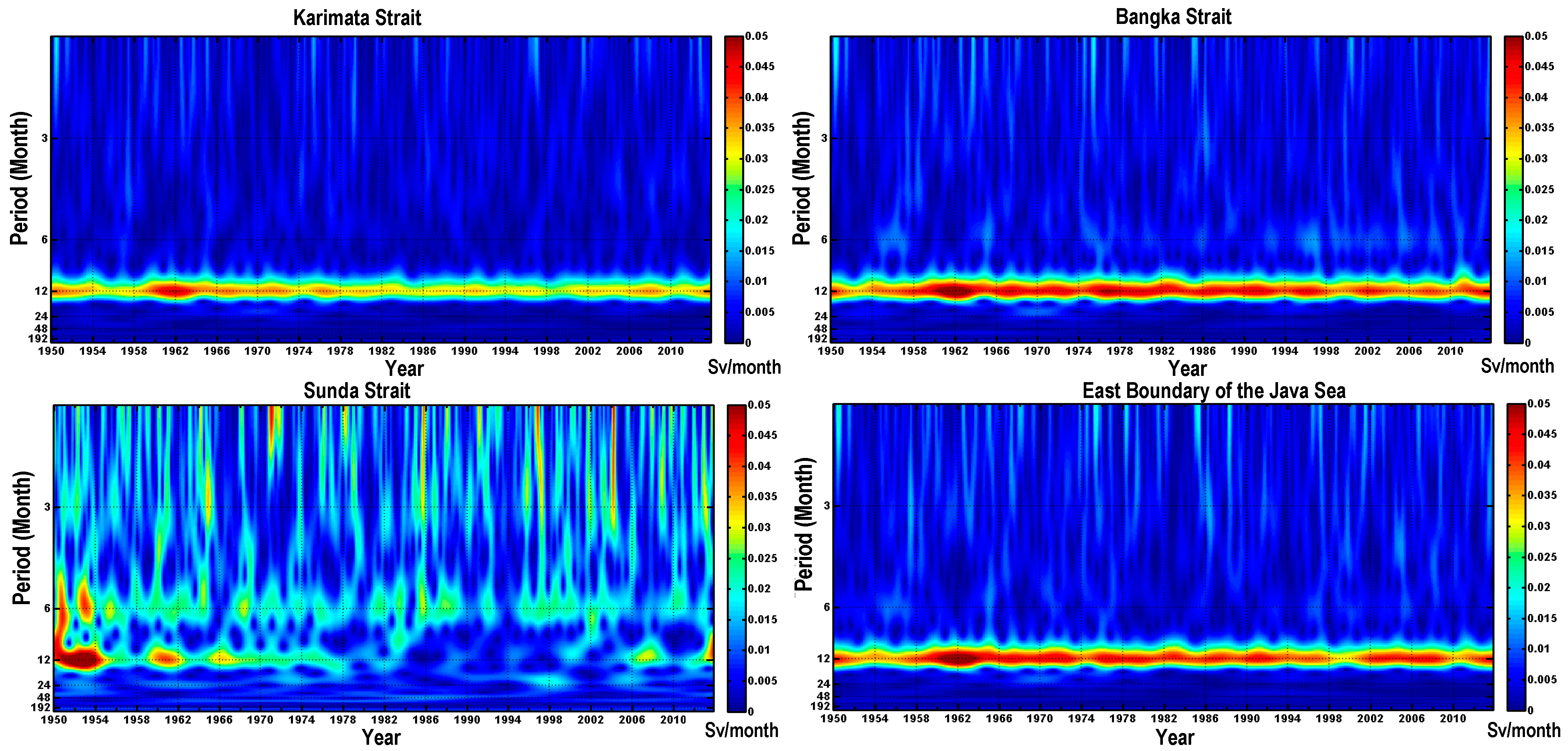
3.3. Time-Frequency Distributions (Power Spectral Density) of the Volume Transport
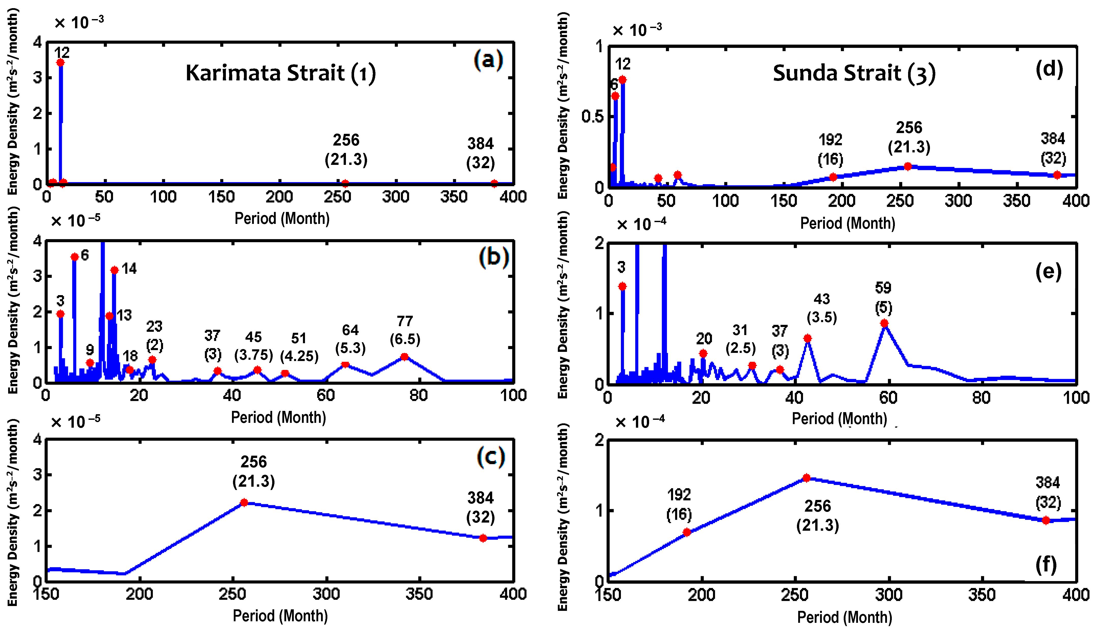
3.4. Energy Spectra of the Volume Transport
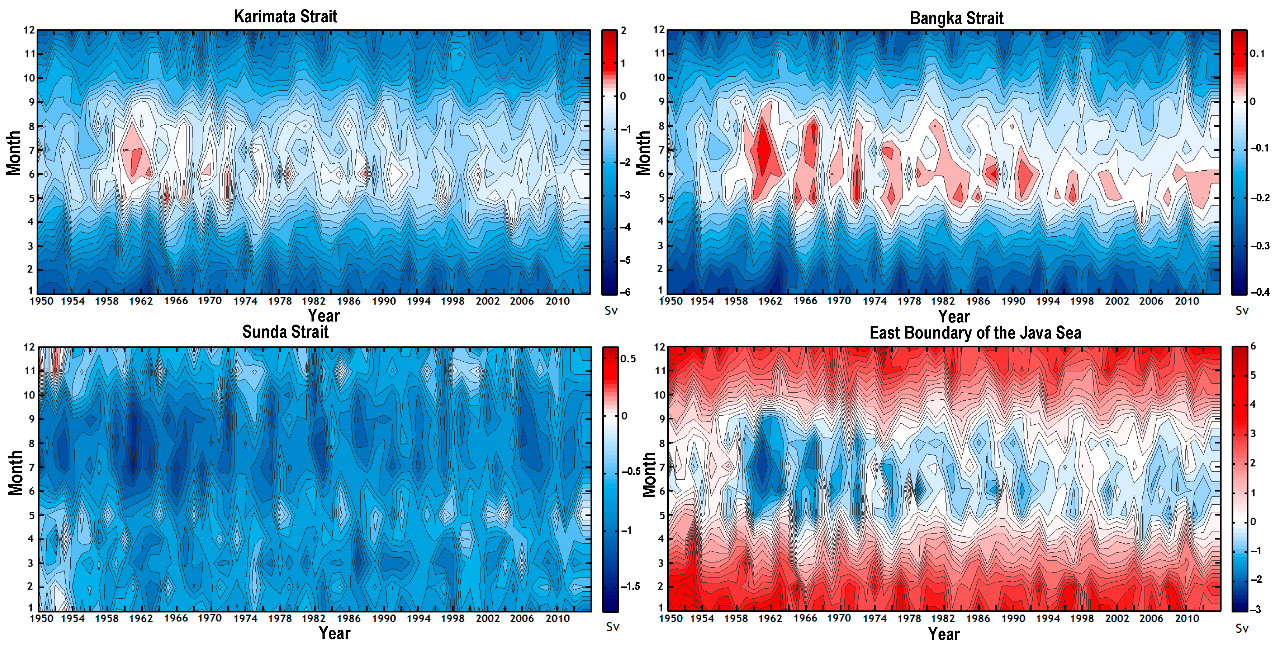
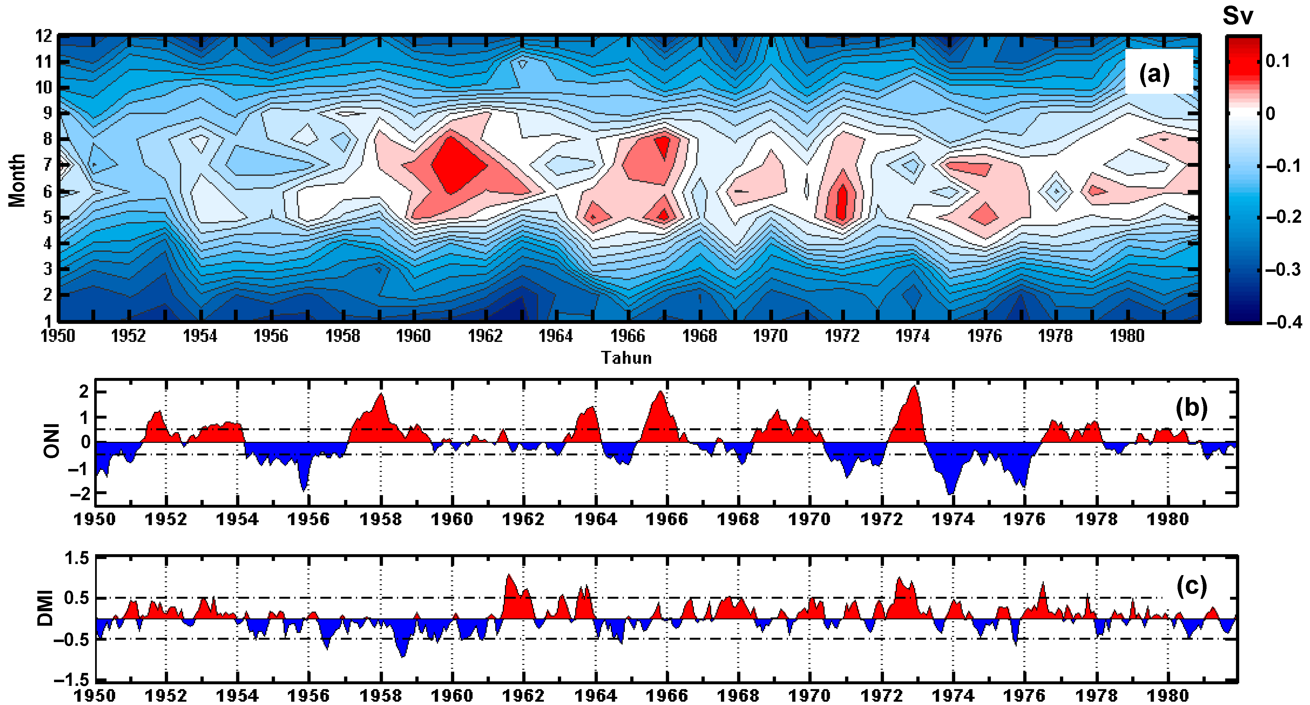
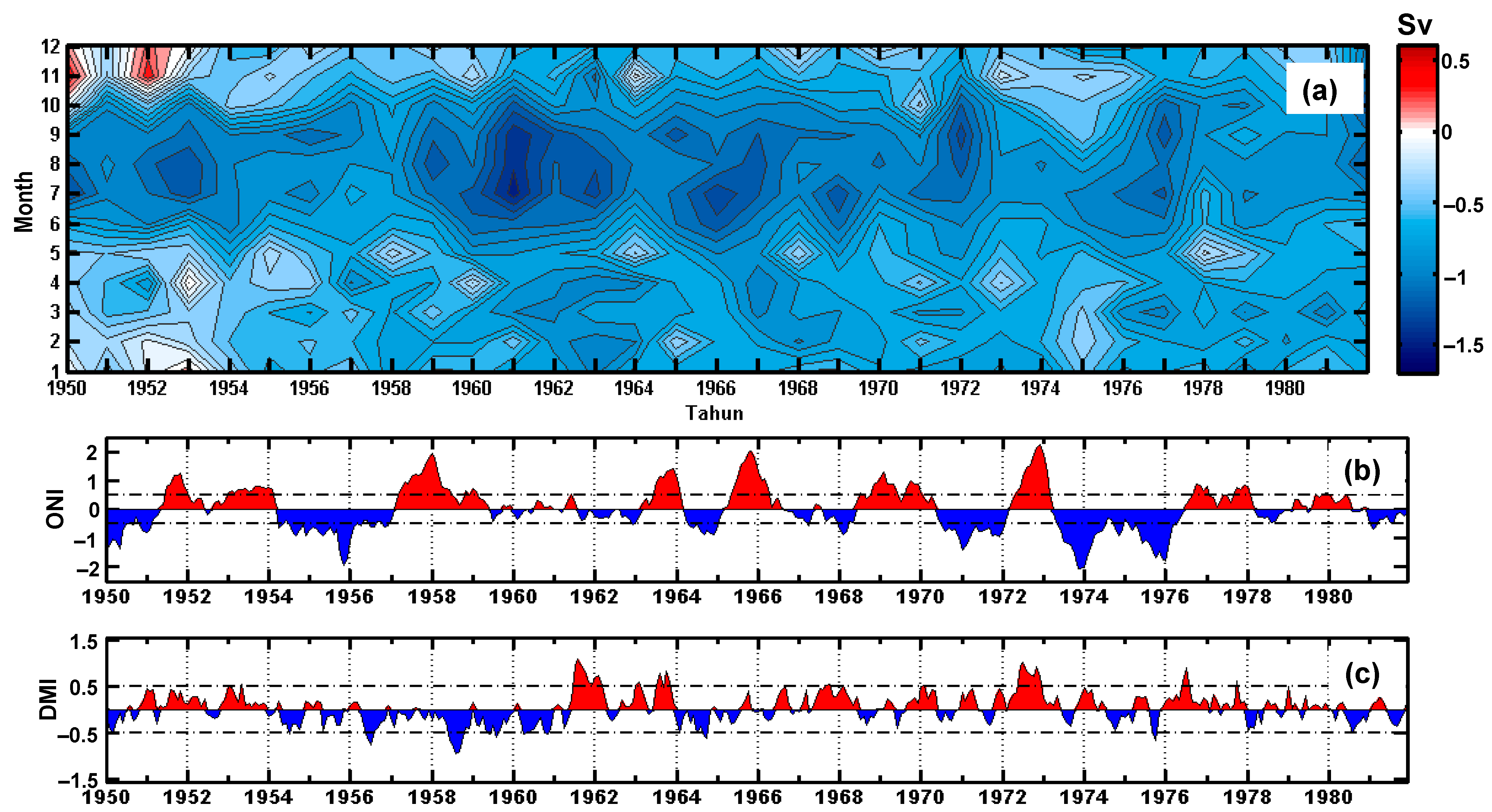
3.5. Monthly and Interannual Variability of the Volume Transport (1950–2013)
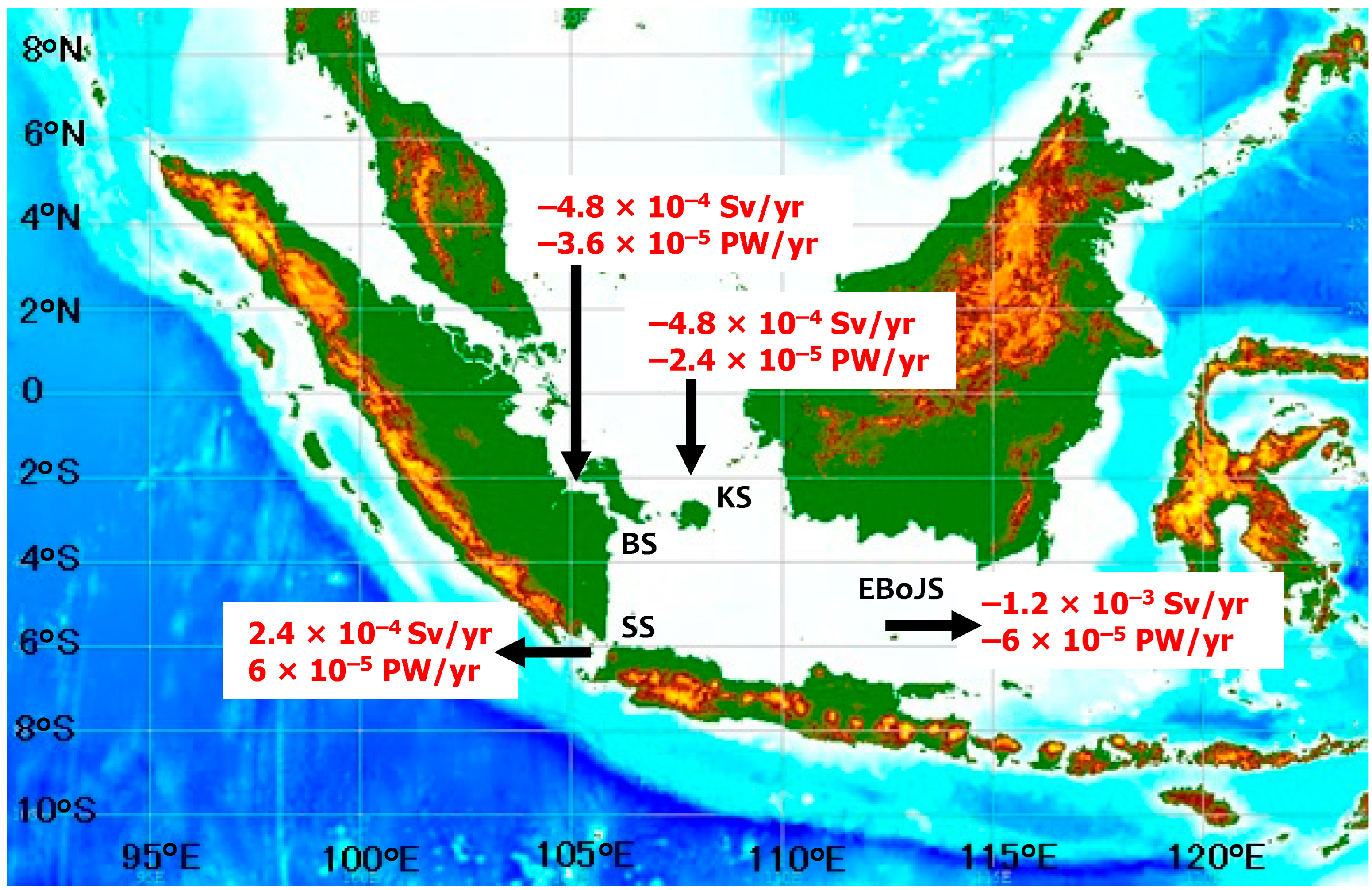
3.6. Long-Term Trend of the Volume Transport and Advective Heat Flux in the Karimata Strait, Sunda Strait, and Eastern Boundary of Java Sea (EBoJS)
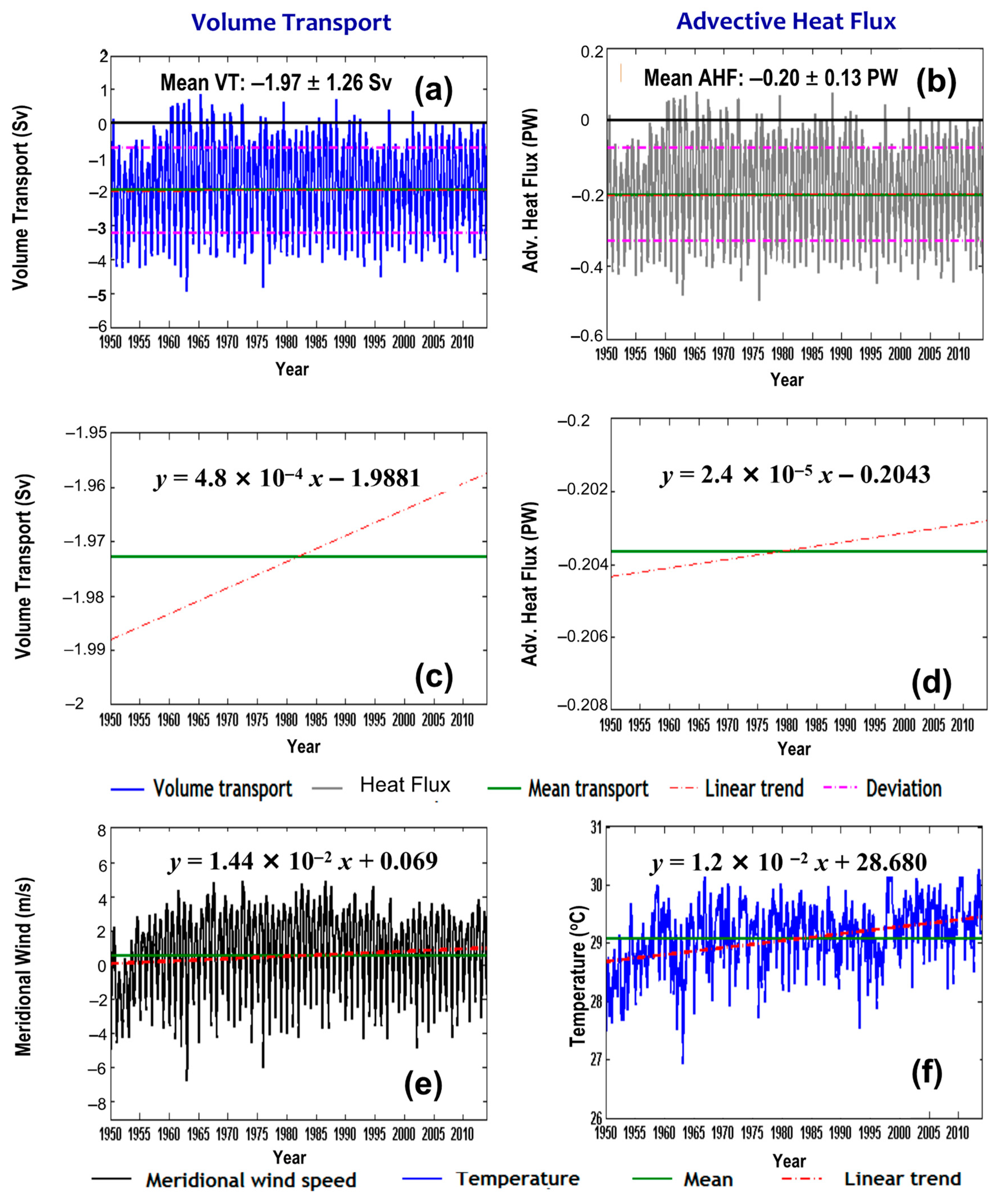
3.6.1. Karimata Strait
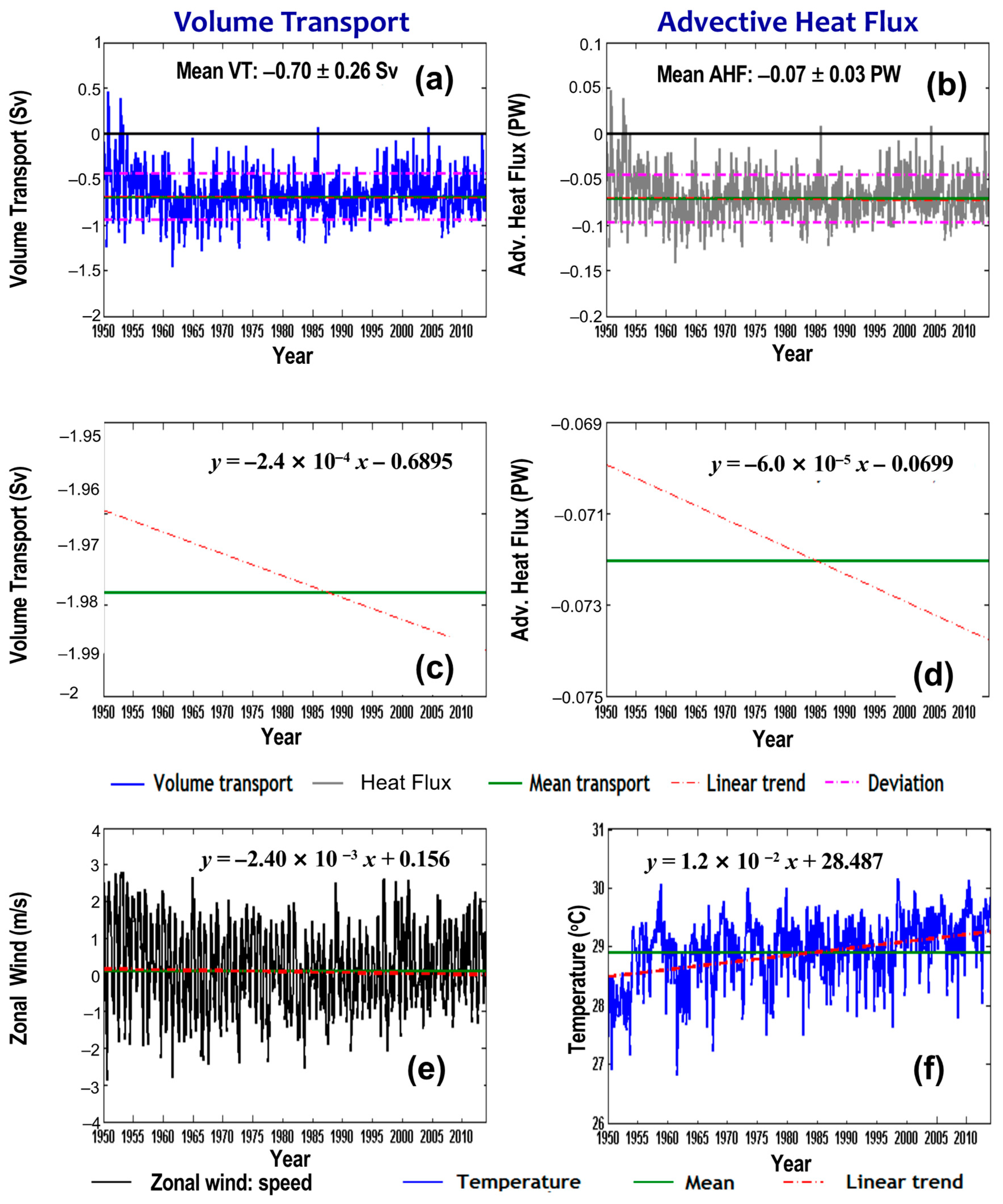
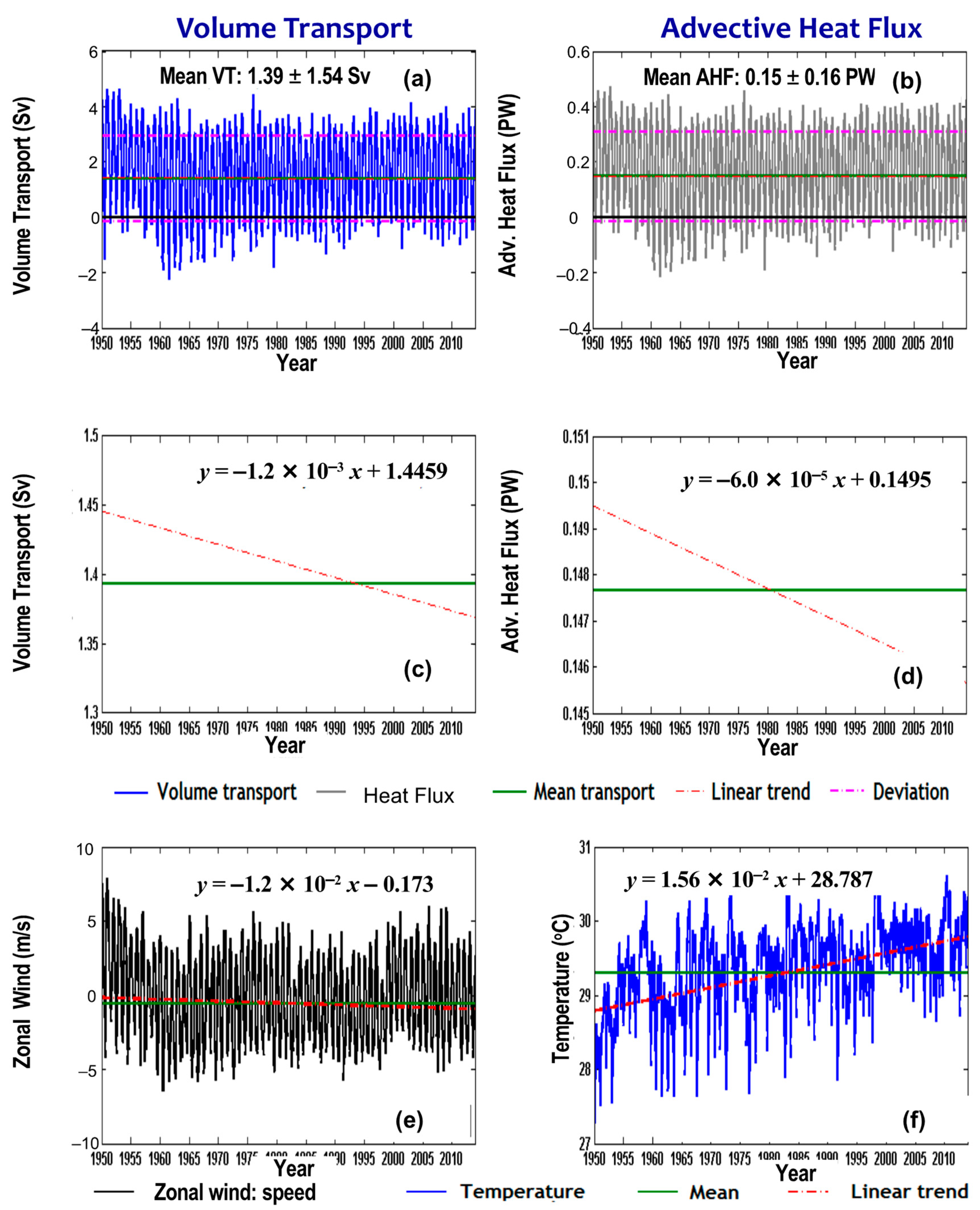
3.6.2. Sunda Strait and Eastern Boundary of Java Sea (EBoJS)
3.7. Interoceanic Volume Transport, Advective Heat Flux, and Heat Budgets
4. Discussion
5. Conclusions
Author Contributions
Funding
Data Availability Statement
Conflicts of Interest
References
- Feng, M.; Zhang, N.; Liu, Q.; Wijffels, S. The Indonesian throughflow, its variability and centennial change. Geosci. Lett. 2018, 5, 3. [Google Scholar] [CrossRef]
- Vranes, K.; Gordon, A.L.; Ffield, A. The heat transport of the Indonesian Throughflow and implications for the Indian Ocean heat budget. Deep. Sea Res. Part II Top. Stud. Oceanogr. 2002, 49, 1391–1410. [Google Scholar] [CrossRef]
- Yari, S.; Kovačević, V.; Cardin, V.; Gačić, M.; Bryden, H.L. Direct estimate of water, heat, and salt transport through the Strait of Otranto. J. Geophys. Res. Ocean. 2012, 117, C9. [Google Scholar] [CrossRef]
- Fang, G.; Wang, Y.; Wei, Z.; Fang, Y.; Qiao, F.; Hu, X. Interocean Circulation and Heat and Freshwater Budgets of the South China Sea Based on a Numerical Model. Dyn. Atmos. Ocean. 2008, 47, 55–72. [Google Scholar] [CrossRef]
- Zheng, Y.; Giese, B. Ocean heat transport in Simple Ocean Data Assimilation: Structure and mechanisms. J. Geophys. Res. 2009, 114, C11009. [Google Scholar] [CrossRef]
- Sprintal, J.; Gordon, A.L.; Wijffels, S.E.; Feng, M.; Hu, S.; Koch-Larrouy, A.; Phillips, H.; Nugroho, D.; Napitu, A.; Pujiana, K.; et al. Detecting Change in the Indonesian Seas. Front. Mar. Sci. 2019, 6, 257. [Google Scholar] [CrossRef]
- Kok, P.H.; Wijeratne, S.; Akhir, M.F.; Ali, F.S.M. Interconnection between the Southern South China Sea and the Java Sea through the Karimata Strait. J. Mar. Sci. Eng. 2021, 9, 1040. [Google Scholar] [CrossRef]
- Susanto, R.D.; Zexun, W.; Rameyo, A.; Bin, F.; Shujiang, L.; Guohong, F. Observations of the Karimata Strait throughflow from December 2007 to November 2008. Acta Oceanol. Sin. 2013, 32, 1–6. [Google Scholar] [CrossRef]
- He, Z.; Feng, M.; Wang, D.; Slawinski, D. Contribution of the Karimata Strait transport to the Indonesian Throughflow as seen from a data assimilation model. Cont. Shelf Res. 2014, 92, 16–22. [Google Scholar] [CrossRef]
- Wei, Z.; Li, S.; Susanto, R.D.; Wang, Y.; Fan, B.; Xu, T.; Sulistiyo, B.; Adi, T.R.; Setiawan, A.; Kuswardani, A.; et al. An overview of 10-year observation of the South China Sea branch of the Pacific to Indian Ocean throughflow at the Karimata Strait. Acta Oceanol. Sin. 2019, 38, 1–11. [Google Scholar] [CrossRef]
- Xu, T.F.; Wei, Z.X.; Susanto, R.D.; Li, S.J.; Wang, Y.G.; Wang, Y. Observed water exchange between the South China Sea and Java Sea through Karimata Strait. J. Geophys. Res. Ocean. 2021, 126, e2020JC016608. [Google Scholar] [CrossRef]
- Gordon, A.L.; Susanto, R.D.; Vranes, K. Cool Indonesian throughflow is a consequence of restricted surface layer flow. Nature 2003, 425, 824–828. [Google Scholar] [CrossRef] [PubMed]
- Fang, G.; Susanto, R.D.; Soesilo, I.; Zheng, Q.; Fangli, Q.; Zexun, W. A note on the South China Sea shallow interocean circulation. Adv. Atmos. Sci. 2005, 22, 946–954. [Google Scholar] [CrossRef]
- Qu, T.; Du, Y.; Meyers, G.; Ishida, A.; Wang, D. Connecting the tropical Pacific with Indian Ocean through South China Sea. Geophys. Res. Lett. 2005, 32, L24609. [Google Scholar] [CrossRef]
- Qu, T.; Meyers, G. Seasonal Characteristics of Circulation in theSoutheastern Tropical Indian Ocean, Notes and Correspondence; American Meteorological Society: Boston, MA, USA, 2005; pp. 255–267. [Google Scholar]
- Wang, D.; Liu, Q.; Huang, R.X.; Du, Y.; Qu, T. Interannual variability of the South China Sea throughflow inferred from wind data and an ocean data assimilation product. Geophys. Res. Lett. 2006, 33, L14605. [Google Scholar] [CrossRef]
- Tozuka, T.; Qu, T.; Yamagata, T. Dramatic impact of the South China Sea on the Indonesian throughflow. Geophys. Res. Lett. 2007, 34, L12612. [Google Scholar] [CrossRef]
- Tozuka, T.; Qu, T.; Masumoto, Y.; Yamagata, T. Impacts of the South China Sea throughflow on seasonal and interannual variations of the Indonesian throughflow. Dyn. Atmos. Oceans 2009, 47, 73–85. [Google Scholar] [CrossRef]
- Fang, G.; Susanto, R.D.; Wirasantosa, S.; Qiao, F.; Supangat, A.; Fan, B.; Wei, Z.; Sulistiyo, B.; Li, S. Volume, Heat, and Freshwater Transports from the South China Sea to Indonesian Seas in the boreal winter of 2007–2008. J. Geophys. Res. 2010, 115, C12020. [Google Scholar] [CrossRef]
- Susanto, R.D.; Fang, G.; Soesilo, I.; Zheng, Q.; Qiao, F.; Wei, Z.; Sulistyo, B. New Surveys of a branch of the Indonesian Throughflow. EOS Trans. AGU 2010, 91, 261–263. [Google Scholar] [CrossRef]
- Gordon, A.L.; Huber, B.A.; Metzger, E.J.; Susanto, R.D.; Hurlburt, H.E.; Adi, T.R. South China Sea Throughflow Impact on the Indonesian Throughflow. Geophys. Res. Lett. 2012, 39, LI1602. [Google Scholar] [CrossRef] [Green Version]
- Suneet, D.; Kumar, M.A.; Atul, S. Upper ocean high resolution regional modeling of the Arabian Sea and Bay of Bengal. Acta Oceanol. Sin. 2019, 38, 32–50. [Google Scholar] [CrossRef]
- Srivastava, A.; Suneet, D.; Mishra, A.K. Investigating the role of air-sea forcing on the variability of hydrography, circulation, and mixed layer depth in the Arabian Sea and Bay of Bengal. Oceanologia 2018, 60, 169–186. [Google Scholar] [CrossRef]
- Han, L.; Zhang, S.; Xu, F.; Lu, J.; Lu, Z.; Ye, G.; Chen, S.; Xu, J.; Du, J. Simulations of sea fog case impacted by air–sea interaction over South China Sea. Front. Mar. Sci. 2022, 9, 1000051. [Google Scholar] [CrossRef]
- Metzger, E.J.; Hurlburt, H.E. Coupled dynamics of the South China sea, the Sulu Sea, and the Pacific ocean. J. Geophys. Res. Ocean. 1996, 101, 12331–12352. [Google Scholar] [CrossRef]
- Lebedev, K.V.; Yaremchuk, M.I. 2000. A diagnostic study of the Indonesian Throughflow. J. Geophys. Res. 2000, 105, 11243–11258. [Google Scholar] [CrossRef]
- Fang, G.; Wei, Z.; Byung-Ho, C.; Kai, W.; Yue, F.; Wei, L. Interbasin freshwater, heat and salt transport through the boundaries of the East and South China Seas from a variable-grid global ocean circulation model. Sci. China Ser. D Earth Sci. 2003, 46, 149–161. [Google Scholar] [CrossRef]
- Gong, D.; Wang, S. Definition of Antarctic Oscillation Index. Geophys. Res. Lett. 1999, 26, 459–462. [Google Scholar] [CrossRef]
- Zhang, Y.; Rossow, W.B.; Stackhouse, P., Jr.; Romanou, A.; Wielicki, B.A. Decadal variations of global energy and ocean heat budget and meridional energy transports inferred from recent global data sets. Clim. Dyn. 2007, 112, D22101. [Google Scholar] [CrossRef]
- Prianto, A. Variability of Mass Transport Across Indonesian and Surrounding Waters. Bachelor Thesis, Oceanography Study Program. Bandung Institute of Technology, Bandung, Indonesia, 2013. [Google Scholar]
- Putri, M.R. Study of Ocean Climate Variability (1959–2002) in the Eastern Indian Ocean, Java Sea and Sunda Strait Using the HAMburg Shelf Ocean Model. Ph.D. Dissertation, Earth Science Department, University of Hamburg, Hamburg, Germany, 2005. [Google Scholar]
- Du, Y.; Qu, T.; Xu, T.; Li, S.; Wei, Z. Three inflow pathways of the Indonesian Throughflow as seen from the simple ocean data assimilation. Dyn. Atmos. Ocean. 2010, 50, 233–256. [Google Scholar] [CrossRef]
- Wang, Y. Seasonal variation of water transport through the Karimata Strait. Acta Oceanol. Sin. Engl. Ed. 2019, 38, 47–57. [Google Scholar] [CrossRef]
- Keerthi, M.G.; Lengaigne, M.; Drushka, K.; Vialard, J.; Montegut, C.D.B.; Pous, S.; Levy, M.; Muraleedharan, P.M. Intraseasonal variability of mixed layer depth in the tropical Indian Ocean. Clim. Dyn. 2016, 46, 2633–2655. [Google Scholar] [CrossRef]
- Keerthi, M.G.; Lengaigne, M.; Vialard, J.; Montégut, C.D.B.; Muraleedharan, P.M. Interannual variability of the Tropical Indian Ocean mixed layer depth. Clim. Dyn. 2013, 40, 743–759. [Google Scholar] [CrossRef]
- Sofian, I. Simulation of The Java Sea Using an Oceanic General Circulation Model. J. Ilm. Geomatika 2007, 13, 1–14. [Google Scholar]
- Sulistya, W.; Hartoko, A.; Prayitno, S.B. The Characteristics and Variability of Sea Surface Temperature in Java Sea; Meteorological and Geophysical Agency: Bali, Indonesia, 2007.
- Nagara, A.N.; Sasongko, N.A.; dan Olakunle, O.J. Introduction to Java Sea; University of Stavanger: Stavanger, Norway, 2007. [Google Scholar]
- Du, Y.; Qu, T.; Meyers, G. Interannual Variability of Sea Surface Temperature off Java and Sumatra in a Global GCM. J. Clim. 2008, 11, 2451–2465. [Google Scholar] [CrossRef]
- Dieterich, C.; Wang, S.; Schimanke, S.; Groger, M.; Klein, B.; Hordoir, R.; Samuelsson, P.; Liu, Y.; Axell, L.; Hoglund, A.; et al. Surface Heat Budget over the North Sea in Climate Change Simulations. Atmosphere 2019, 10, 272. [Google Scholar] [CrossRef]
- Wirasatriya, A.; Sugianto, D.N.; Helmi, M.; Maslukah, L.; Widiyandono, R.T.; Herawati, V.E.; Subardjo, P.; Handoyo, G.; Marwoto, J.; Suryoputro, A.A.D.; et al. Heat Flux Aspects on The Seasonal Variability of Sea Surface Temperature in The Java Sea. Ecol. Environ. Conserv. Pap. 2019, 25, 434–442. [Google Scholar]
- IOC; IHO; dan BODC. General Bathymetric Chart of the Ocean. Centenary Edition of the GEBCO Digital Atlas; BODC: Liverpool, UK, 2003.
- Smith, W.H.F.; Sandwell, D.T. Global Sea Floor Topography from Satellite Altimetry and Ship Depth Soundings. Science 1997, 277, 1956. [Google Scholar] [CrossRef]
- Conkright, M.E.; Levitus, S.; Boyer, T.P. World Ocean Atlas 1994 Volume 1: Nutrients; NOAA: Washington, DC, USA, 1994.
- Levitus, S.; Boyer, T.P. World Ocean Atlas 1994 Volume 2: Oxygen; NOAA: Washington, DC, USA, 1994.
- Levitus, S.; Burgett, R.; Boyer, T.P. World Ocean Atlas 1994 Volume 3: Nutrients; NOAA: Washington, DC, USA, 1994.
- Levitus, S.; Boyer, T.P. World Ocean Atlas 1994 Volume 4: Temperature; NOAA: Washington, DC, USA, 1994.
- Kanamitsu, M.; Ebisuzaki, W.; Woolen, J.; Yang, S.-K.; Hnilo, J.J.; Fiorino, M.; Potter, G.L. NCEP–DOE AMIP-II Reanalysis (R-2). Am. Meteorol. Soc. J. 2002, 83, 1631–1644. [Google Scholar] [CrossRef]
- Hanifah, F.; Ningsih, N.S.; Sofian, I. Dynamics of eddies in the southeastern tropical Indian Oceean. J. Phys. Conf. Ser. 2016, 739, 012042. [Google Scholar] [CrossRef]
- Hanifah, F.; Ningsih, N.S. The characteristic of eddies in the Banda Sea. Adv. Appl. Fluid Mech. 2016, 19, 889. [Google Scholar] [CrossRef]
- Ningsih, N.S.; Azhar, M.A.; Hanifah, F.; Kushadiwijayanto, A.A. Eddy Variability Study to Identify Water Fertility as an Effort to Strengthen National Food Security (Case Study: Java’s Southern Waters); ITB Batch II Research and Innovation Program Report; Bandung Institute of Technology: Bandung, Indonesia, 2014. [Google Scholar]
- Ningsih, N.S.; Sakina, S.L.; Susanto, R.D.; Hanifah, F. Simulated zonal current characteristics in the southeastern tropical Indian Ocean (SETIO). Ocean Sci. 2021, 17, 1115–1140. [Google Scholar] [CrossRef]
- Wannasingha, U.; Webb, D.J.; de Cuevas, B.A.; Coward, A.C. On the Indonesian Throughflow in the OCCAM Model. 2003. Available online: http://www.noc.soton.ac.uk/ (accessed on 7 April 2015).
- Yaremchuk, M.; McCreary, J.; Yu, Z.; Furue, R. The South China Sea throughflow retrieved from climatological data. J. Phys. Oceanogr. 2009, 39, 753–767. [Google Scholar] [CrossRef]
- Susanto, R.D.; Wei, Z.; Adi, T.R.; Zheng, Q.; Fang, G.; Fan, B.; Supangat, A.; Agustiadi, T.; Li, S.; Trenggono, M.; et al. Oceanography surrounding Krakatau Volcano in the Sunda Strait, Indonesia. Oceanography 2016, 2, 228–237. [Google Scholar]
- Syamsudin, F.; Kaneko, A. Numerical and Observational Estimates of Indian Ocean Kelvin Wave Intrusion into Lombok Strait. Hiroshima University. Geophys. Res. Lett. 2004, 31, L24307. [Google Scholar] [CrossRef]
- Iskandar, I.; Mardiansyah, W.; Matsumoto, Y.; Yamagata, T. Intraseasonal Kelvin Waves Along The Southern Coast of Sumatra and Java. J. Geophys. Res. 2005, 110, C04013. [Google Scholar] [CrossRef]
- Goswami, B.N.; Xavier, P.K. ENSO control on the south Asian monsoon through the length of the rainy season. Geophys. Res. Lett. 2005, 32, L18717. [Google Scholar] [CrossRef] [Green Version]


| Parameter | Resolution | Period | Source | References | |
|---|---|---|---|---|---|
| Model Input | Bathymetry | 2′ | - | ETOPO2 | [43] |
| Temperature | - | - | LEVITUS94 | [44,45,46,47] | |
| Salinity | |||||
| Air Temperature | 1875° | 1949–2013 | NCEP Reanalysis | [48] | |
| Humidity | |||||
| Rainfall | |||||
| Solar Radiation | |||||
| Wind | |||||
| SST (assimilation) | 1875° | 1949–2013 | NCEP Reanalysis | [48] | |
| Verification | Surface Current | 1° | 1993–2013 | Ocean Surface Current Analyses (OSCAR) | [49,50] |
| SSHA | 1/3° | 1993–2010 | AVISO | ||
| SST | 2° | 1949–2013 | NOAA |
| Global Model | Regional Model | |
|---|---|---|
| Model Domain | 60° S–60° N and 180° W–180 VE | 21.5° S–23° N and 90° E–139° E |
| Resolution | 1/2° | 1/8° |
| Layer | 22 | 22 |
| Bathymetry | ETOPO2 (2′ resolution) | ETOPO2 (2′ resolution) + DISHIDROS map |
| Simulation Period | 64 years (1950–2013) | 64 years (1950–2013) |
| Source | Volume Transports (Sv = 106 m3/s) | Period of Data | Method | |||
|---|---|---|---|---|---|---|
| Karimata Strait (1) | Bangka Strait (2) | Sunda Strait (3) | Eastern Boundary of the Java Sea (4) | |||
| [53] | −0.30 | 1992–2000 (9 years) | Numerical Model (OCCAM, 1/4°) | |||
| [26] | −2.10 | Numerical Model | ||||
| [31] | −1.01 | −0.62 | 0.29 | 1959–2002 (44 years) | Numerical Model (HAMSOM, 1/6°) | |
| [13] | −1.30 | Numerical Model | ||||
| [4] | −1.16 | 1982–2003 (22 years) | Numerical Model (1/6°) | |||
| [54] | −0.30 | Numerical Model | ||||
| [18] | −1.60 | Numerical Model | ||||
| [19] | −0.80 | December 2007–November 2008 (1 year) | Roughly estimate from ADCP measurement | |||
| [21] | −0.58 | 2003–2010 (8 years) | Numerical Model (HYCOM, 1/12.5°) | |||
| [30] | −0.87 | −0.12 | 0.70 | 1950–2011 (62 years) | Numerical Model (HYCOM, 1/4°) | |
| [8] | −0.50 | November 2008–October 2009 | ADCP measurement | |||
| [55] | 0.24 (the boreal winter)/−0.83 (the boreal summer) | 2008–2009 | ADCP measurement | |||
| Present Study (2017) | −1.97 | −0.12 | −0.70 | 1.39 | 1950–2013 (64 years) | Numerical Model (HYCOM, 1/8°) |
| Source | Advective Heat Flux (PW = 1015 W) | Period of Data | Method | Notes | |||
|---|---|---|---|---|---|---|---|
| Karimata Strait (1) | Bangka Strait (2) | Sunda Strait (3) | Eastern Boundary of the Java Sea (4) | ||||
| [4] | −0.113 | 1982–2003 (22 years) | Numerical Model (1/6°) | Annual mean value | |||
| [19] | −0.360 | December 2007–November 2008 (1 year) | Roughly estimate from ADCP measurement | In the boreal winter month | |||
| [8] | −0.05 | November 2008–October 2009 | ADCP measurement | Annual mean value | |||
| Present Study (2017) | −0.204 | −0.012 | −0.072 | 0.148 | 1950–2013 (64 years) | Numerical Model (HYCOM, 1/8°) | Annual mean value |
| The Java Sea Interoceanic Passages | Direction of Transports | In the Period 1950–2013 (64 Years) | |
|---|---|---|---|
| Total Increase (+ Value)/Decrease (− Value) | |||
| Volume Transport (Sv) | Advective Heat Flux (PW) | ||
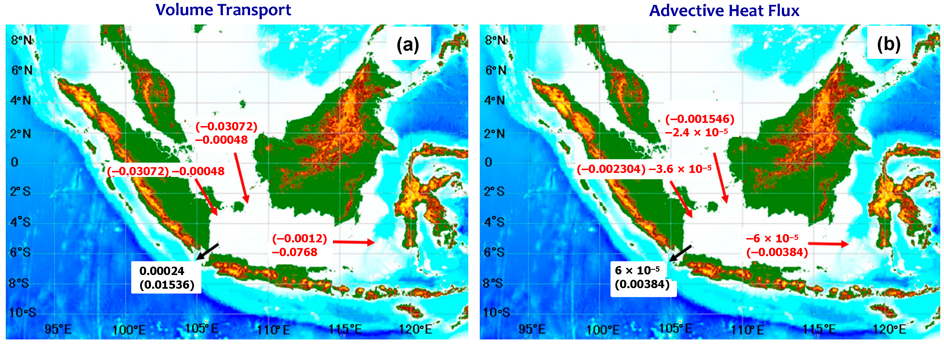
| Eastern Boundary of Java Sea | Outflow | −0.07680 | −0.00384 |
| Karimata and Bangka Strait | Inflow | −0.06144 | −0.00385 |
| Sunda Strait | Outflow | 0.01536 | 0.00384 |
| The Java Sea Interoceanic Passages | Mean Volume Transport (Sv) | Percentage (%) | Description |
|---|---|---|---|
| Karimata Strait | 1.97 | 94.26 | inflow |
| Bangka Strait | 0.12 | 5.74 | inflow |
| Sunda Strait | −0.70 | 33.50 | outflow |
| East Boundary of Java Strait | −1.39 | 66.50 | outflow |
| Inflow–Outflow | 0.00 | 0.00 | outflow = inflow |
| The Java Sea Interoceanic Passages | Mean Advective Heat Flux (PW) | Percentage (%) | Description |
|---|---|---|---|
| Karimata Strait | 0.204 | 92.73 | inflow |
| Bangka Strait | 0.012 | 5.45 | inflow |
| Sunda Strait | −0.072 | 32.73 | outflow |
| East Boundary of Java Sea | −0.148 | 67.27 | outflow |
| Inflow-Outflow | −0.004 | 1.82 | outflow > inflow |
| The Java Sea Interoceanic Passages | El Niño | La Niña | Dipole Mode + | Dipole Mode – |
|---|---|---|---|---|
| The Karimata Strait and Bangka Strait | Southward transport (ST) reduces | ST enhances | ST enhances | ST reduces |
| The Sunda Strait | Westward transport (WT) reduces | WT enhances | WT enhances | WT reduces |
| The Eastern Boundary of Java Sea | Eastward transport (ET) enhances | ET reduces | ET reduces | ET enhances |
Disclaimer/Publisher’s Note: The statements, opinions and data contained in all publications are solely those of the individual author(s) and contributor(s) and not of MDPI and/or the editor(s). MDPI and/or the editor(s) disclaim responsibility for any injury to people or property resulting from any ideas, methods, instructions or products referred to in the content. |
© 2023 by the authors. Licensee MDPI, Basel, Switzerland. This article is an open access article distributed under the terms and conditions of the Creative Commons Attribution (CC BY) license (https://creativecommons.org/licenses/by/4.0/).
Share and Cite
Rachmayani, R.; Ningsih, N.S.; Hanifah, F.; Nabilla, Y. Long-Term Trend and Variability of Volume Transport and Advective Heat Flux through the Boundaries of the Java Sea Based on a Global Ocean Circulation Model (1950–2013). Water 2023, 15, 740. https://doi.org/10.3390/w15040740
Rachmayani R, Ningsih NS, Hanifah F, Nabilla Y. Long-Term Trend and Variability of Volume Transport and Advective Heat Flux through the Boundaries of the Java Sea Based on a Global Ocean Circulation Model (1950–2013). Water. 2023; 15(4):740. https://doi.org/10.3390/w15040740
Chicago/Turabian StyleRachmayani, Rima, Nining Sari Ningsih, Farrah Hanifah, and Yasmin Nabilla. 2023. "Long-Term Trend and Variability of Volume Transport and Advective Heat Flux through the Boundaries of the Java Sea Based on a Global Ocean Circulation Model (1950–2013)" Water 15, no. 4: 740. https://doi.org/10.3390/w15040740