Assessing the Influence of a Bias Correction Method on Future Climate Scenarios Using SWAT as an Impact Model Indicator

Abstract

In this study, we evaluate the implications of a bias correction method on a combination of Global/Regional Climate Models (GCM and RCM) for simulating precipitation and, subsequently, streamflow, surface runoff, and water yield in the Soil and Water Assessment Tool (SWAT). The study area is the Des Moines River Basin, U.S.A. The climate projections are two RCMs driven by two GCMs for historical simulations (1981–2005) and future projections (2030–2050). Bias correction improves historical precipitation for annual volumes, seasonality, spatial distribution, and mean error. Simulated monthly historical streamflow was compared across 26 monitoring stations with mostly satisfactory results for percent bias (Pbias). There were no changes in annual trends for future scenarios except for raw WRF models. Seasonal variability remained the same; however, most models predicted an increase in monthly precipitation from January to March and a reduction for June and July. Meanwhile, the bias-corrected models showed changes in prediction signals. In some cases, raw models projected an increase in surface runoff and water yield, but the bias-corrected models projected a reduction in these variables. This suggests the bias correction may be larger than the climate-change signal and indicates the procedure is not a small correction but a major factor.

1. Introduction

Global Climate Models (GCM) represent the terrestrial climate system based on the conservation laws of mass, energy, and momentum and laws of thermodynamics and radiation [1]. They are divided into simulations of historical (e.g., 1950–2005) and future scenarios (e.g., 2020–2099) of climate variables such as precipitation, temperature, and humidity [2]. GCM simulations of future climate use Representative Concentration Pathways (RCPs), which are based on variations in population growth, lifestyle and behavior, land use, technology, and climate policies. The RCPs describe different possibilities for atmospheric emissions and concentrations. The scenario with very high greenhouse gas emissions is the RCP 8.5 [3] and is the one chosen for this study. The choice is justified by the fact that this scenario showed the closest agreement between historical emissions (compared to historical data through the year 2020) and anticipated outcomes of mid-century current global climate policies [4]. Regional Climate Models (RCMs) use dynamic downscaling methods to provide climate information on finer scales than GCMs, while still preserving the laws of physics [5]. Thus, RCMs add simulation value but do not replace GCMs.

Coupling climatic models together with other models, such as the Soil and Water Assessment Tool (SWAT) ecohydrological model [6,7,8], is not a new approach, and their widespread use demonstrates a wide variety of methodologies and applications. Some of the common topics in these types of studies are (a) techniques of downscaling and bias correction [9,10,11], (b) climate models’ spatial resolution [12], (c) impact models application [13,14], and (d) land use change impacts [15,16,17].

Precipitation is the main driver of the hydrologic cycle and is a critical resource for socioeconomic activities. Impacts caused by either an absence or excess of water (droughts or floods) result in more damage worldwide than any other natural hazard, and their risks may be exacerbated by climate change and socioeconomic activities [18]. In Iowa, USA, climate change is reflected in recent changes in rainfall, humidity, and temperature patterns. Projections show an increase in precipitation in winter, a decrease in summer, and an expectation of much warmer summers, with 5 to 15 days each year having a heat index over 106 °F by 2050 [19]. An increase in the number of intense rainfall events is another relevant factor since this has a large impact on agricultural systems that play a crucial economic role in the region. High-intensity rainfall can result in increased soil erosion and compromise agricultural production [20]. A spatially distributed and physically-based modeling system (GCM-RCM-Impact/Ecohydrological model) offers the potential to assess the impacts of future changes on climate and their consequences for water balance responses [13,15].

According to previous research, data simulated by climate models, such as precipitation, should be used cautiously, as they may show significant biases [11,21]. Some reasons for such biases include model errors caused by imperfect conceptualization and discretization, and among solutions, authors recommend using bias correction methods. However, whether or not to apply a bias correction method to a GCM-RCM simulation is still a topic under discussion, and care should be taken when correcting the noise. An acceptable threshold for the magnitude of bias correction that will not affect future RCM projection behavior is unknown. Non-corrected models can lead to unrealistic precipitation magnitudes [14], but corrections add another step to the process and could increase uncertainty [22,23]. Integrating the outputs of ecohydrological models with climate models is a very challenging task, and few studies have systematically demonstrated the limitations of climate models in representing rainfall conditions for ecohydrological studies at a regional scale.

In this study, we evaluated the application of a bias-correction technique (distribution mapping) to precipitation datasets from two GCMs and two RCMs combined for analyses of the Des Moines River Basin (DMRB) that drains parts of Minnesota and Iowa. The analysis was based on the combined use of climate models with the SWAT model to analyze streamflow, surface runoff, and water yield. This analysis builds directly on a previous SWAT DMRB application [24] and on the extensive use of SWAT in the U.S. Corn Belt region as well as other regions worldwide [25,26,27]. The specific objectives of the study were to (1) assess both raw and bias-corrected GCM-RCM data for replication of historical (1981–2005) DMRB streamflow and other hydrological indicators simulated in SWAT, and (2) evaluate the hydrological impacts of the RCP 8.5 scenario on the DMRB for the future period of 2030–2049.

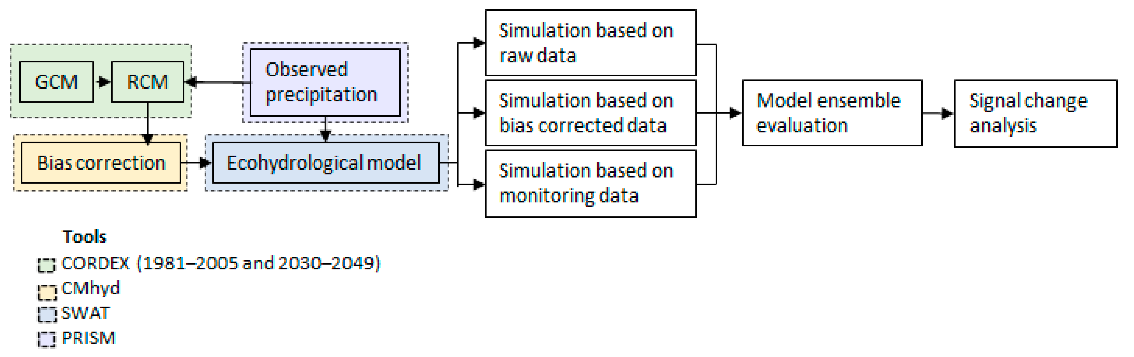
2. Materials and Methods

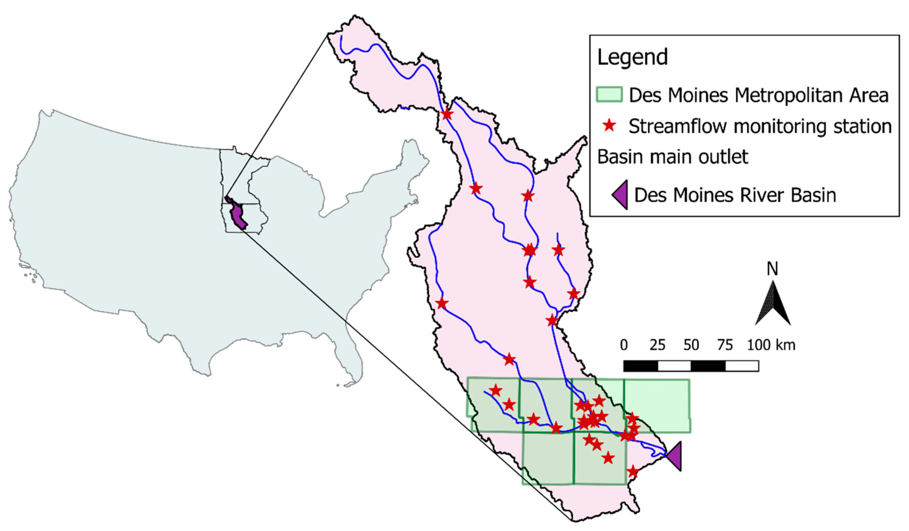
2.1. Study Area

The study area encompassed the portion of the DMRB (31,892.4 km²) that drains from southern Minnesota to south central Iowa (Figure 1). Land use in the DMRB is dominated by agricultural row crop systems (70%) consisting primarily of soybean and corn production (additional land use data has been previously reported [24]). The DRMB cropland landscapes are intensely managed with subsurface tile drains (54% of the total basin area). The basin drains to the Des Moines Metropolitan Statistical Area (DMMSA), which is the densest urban area in Iowa (8% of the total basin area, Figure 1). The major soil types are Udolls (freely-drained Mollisols), Aquolls (wet Mollisols), and Udalfs (Alfisols) [28]. According to the Köppen classification, the climate is Dfa [29] (humid continental conditions with hot summers and cold winters). The annual mean (based on data from 1985 to 2018) precipitation, evapotranspiration, and surface runoff are 873 mm, 670 mm, and 68 mm, respectively (additional description of the DMRB has been provided [24]).

2.2. Climate Models and SWAT Ecohydrological Model

We evaluated monthly projections of two Global Climate Models (MPI-ESM-LR and GFDL-ESM2M) coupled with two Regional Climate Models (WRF and RegCM4) and the RCP Scenario 8.5 for a future period of 2030–2049 [30]. Corresponding data for the historical period 1981–2005 were used as input for the SWAT model to identify hydrological climate change signals with a focus on surface runoff and water yield. Model integration occurred when the output data of a coupled GCM-RCM (precipitation) were used as input data for the SWAT model. The bias correction effect was assessed by correcting projected precipitation and comparing results for the historical and future runs, and climate change signals with those obtained using a non-corrected (raw) climate scenario (Figure 2).

We used the Parameter-Elevation Relationships on Independent Slopes Model (PRISM) dataset [31] to obtain observed precipitation for model evaluation. Observed streamflow data used to evaluate the accuracy of the hydrological modeling was selected from the USGS database [32]. There were 26 monitoring gauges selected in the study area (Figure 1) with a time series of 10 years or more of data recorded. The data were downloaded at a daily scale and subsequently aggregated into a monthly time step.

2.2.1. Climate Models and the CORDEX Platform

RCMs are downscaling models driven by GCMs, where the GCM outputs serve as the boundary conditions for the RCMs. The relationships are established between large-scale predictors and regional-to-local scale predictands. This GCM to RCM procedure provides information on a much finer spatial scale, e.g., converting GCM output from a ~100–km × 100–km scale to a refined 25–km × 25–km scale [30]. The Coordinated Regional Climate Downscaling Experiment (CORDEX) platform was developed by the Task Force on Regional Climate Downscaling and supported by the World Climate Research Programme (WRCP), which uses climate simulations from the Coupled Model Intercomparison Project (CMIP 5) archive [33]. This collaborative initiative has the purpose of supporting model evaluation for performance and climate projections within a specific domain [34].

The climate data were accessed via the NA-CORDEX portal [35], which provides 58 GCM-RCM combinations for the North American domain at a 0.44° and 0.22° resolution [36]. Of all models, 35 are available for the historical run and RCP 8.5 [35]. We chose two models (at 0.22° resolution) for this study (

Table 1. Description of model type, modeling center, and resolution for the Global Climate Models (GCM) and Regional Climate Models (RCM); for this study, two RCMs are driven by two GCMs for a total of four evaluations.

Model	Type	Modeling Centers	Resolution a
MPI-ESM-LR	GCM	Max Planck Institute for Meteorology Earth System Model	1.90°
GFDL-ESM2M	GCM	National Oceanic and Atmospheric Administration/Geophysical Fluid Dynamics Laboratory	2.45°
WRF	RCM	National Center for Atmospheric Research	0.44°/0.22°
RegCM4 b	RCM	International Center for Theoretical Physics	0.44°/0.22°

Notes: ^a Source: [29,36]; ^b [37].

). Temperature predictions generated by climate models are more reliable and show less bias [11,21]. In this study, we evaluated only the effects of precipitation on the hydrological variables.

2.2.2. SWAT Ecohydrological Model

The SWAT model is a distributed ecohydrological model continuous in time and space developed to explore the effects of climate and land management practices on water resources [6,7,8,38]. The hydrological part of the model is based on a water balance equation for the soil profile that includes precipitation, surface runoff, infiltration, evapotranspiration, lateral flow, percolation, and groundwater movement processes. The simulation unit of the model, a Hydrological Response Unit (HRU), is defined as an area comprised of unique land cover, management, soil type, and topography within a subwatershed [39,40]. The model used in this study was built using “real system data” (or soft data) as previously described [24]. The model was run with a daily time step, and the results were analyzed monthly. The runoff was calculated with the Curve Number (CN) method, and channel routing was calculated using the Variable Storage method. The Penman–Monteith equation was used to calculate potential evapotranspiration. In this study, the output variables analyzed (monthly time step) were surface runoff and water yield for current and future climate and streamflow for the historical run only. The procedure of driving the SWAT model with the climate model projections was the same as that for historical monitoring data, and precipitation was the only variable that changed between simulations. The eight models we developed were then analyzed and compared to each other.

2.2.3. Bias Correction

Bias correction is a common practice when using climate models as input to ecohydrological models due to GCM-RCM’s imperfect conceptualization, discretization, and spatial averaging at very coarse resolutions [14,41,42]. Bias correction methods are assumed to be stationary; thus, the same parametrized correction algorithm applied for historical data is applied to future climate data. Even though good historical performance does not mean good future performance, a method that works well under current conditions is likely to perform better under changed conditions than a method that works poorly under current conditions [11,41]. We selected the Distribution Mapping (DM) bias correction method [21] to correct the statistical distribution function of the values simulated by the GCM-RCM relative to the distribution function of the observed data for precipitation. This approach goes by several names, such as probability mapping, quantile–quantile mapping, statistical downscaling, or histogram equalization [11,43], and the method is widely used for this type of application [42]. The DM is applied with a Gamma distribution as a function of parameter shape (which controls the distribution profile) and scale (which determines the dispersion of the distribution) to adjust precipitation events (Equation (1)):

$$f_y\left(x|\alpha ,\beta \right)=x^{\alpha -1}\times \frac{1}{{\beta }^{\alpha }\times \Gamma \left(\alpha \right)}\times e^{\frac{-x}{\beta }}|x\ge 0;\alpha ,\beta >0$$

(1)

where α is the shape parameter and β is the scale parameter, x is the random variable (precipitation).

Advantages of using the DM include correction of the mean, standard deviation, frequency, and intensity of humid days and events in a non-linear way [11,14,21]. Disadvantages, such as inflation-related problems, can occur if the simulated and observed grids do not have the same horizontal resolution [44,45].

The CMhyd platform [41] was used to apply the DM to the DMRB precipitation data. This program has eight bias correction methods for precipitation and temperature data and provides output files in a SWAT model format. The bias correction was applied for historical (1981–2005) and future (2030–2050) time-series data. The observed data from the ~4 km PRISM dataset grid were averaged for a ~10 km grid. The 10 km spatial discretization corresponds to the 12-digit [46] subbasin division used in the SWAT model simulations. In other words, each subbasin has a unique precipitation value. These data were added to the CMhyd platform to perform bias correction. The CMhyd selects the closest observed station to the climate model grid cells to compare observed and simulated historical time series, i.e., the grid size considered in the bias correction process is the same for observed and MPI-ESM-LR-RegCM4, GFDL-ESM2M-RegCM4, MPI-ESM-LR-WRF, GFDL-ESM2M-WRF climate models, ~25 km.

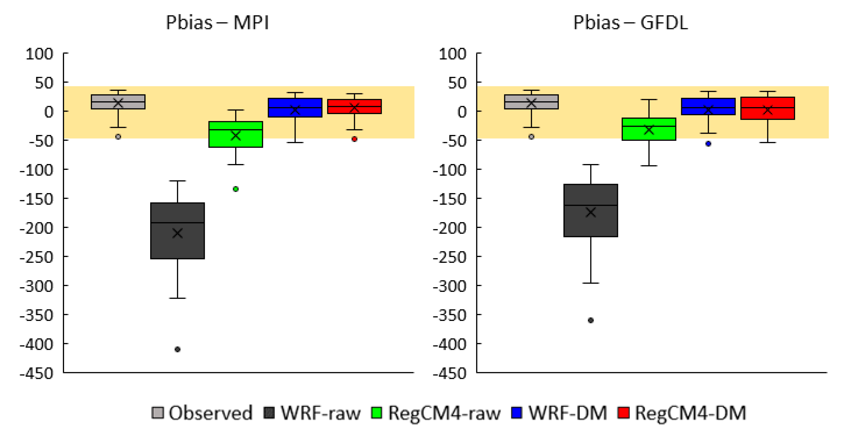
2.3. Statistical Evaluation

Differences for model precipitation were quantified using four statistical coefficients, including root mean square error (RMSE, Equation (2)), mean error (ME, Equation (3)), relative bias (BIAS, Equation (4)), and standard deviation (STDE, Equation (5)). The RMSE is a standard statistical metric to measure model performance in fields such as meteorology and climate studies [47]; the RMSE results are the average distance between simulated and observed values, and the metric does not indicate bias [48]. For both RMSE and ME, the lower the value, the better the fit, and 0 is the ideal result; ME ranges from −∞ to ∞ and RMSE from 0 to ∞. Relative bias (BIAS) measures systematic errors in calculating the differences between the precipitation datasets [49].

The Pbias (Equation (6)) evaluates the trend for the average of simulated values in relation to observed values and is widely used for hydrological evaluations [50,51]. Considering the SWAT model outputs ideal Pbias value is zero (%); a good model performance could be ±25% for streamflow. Positive values indicate model underestimation, and negative values indicate overestimation [50,51].

$$RMSE=\sqrt{\frac{1}{n}{\displaystyle \sum }_{i=1}^n{\left(X_i^{obs}-X_i^{sim}\right)}^2}$$

(2)

$$ME=\frac{1}{n}{\displaystyle \sum }_{i=1}^n\left(X_i^{obs}-X_i^{sim}\right)$$

(3)

$$BIAS=\left[\frac{{{\displaystyle \sum }}_{t=1}^n\left(X_i^{obs}-X_i^{sim}\right)}{{{\displaystyle \sum }}_{t=1}^n\left(X_i^{obs}\right)}\right]\times 100$$

(4)

$$STDE=\frac{\sqrt{{{\displaystyle \sum }}_i^n{P}_i}}{n}$$

(5)

$$Pbias=\left[\frac{{{\displaystyle \sum }}_{t=1}^n{\left(X_i^{obs}-X_i^{sim}\right)}^2}{{{\displaystyle \sum }}_{t=1}^n\left(X_i^{obs}\right)}\right]\times 100$$

(6)

where $X_i^{sim}$ are simulated values of the ith day, and $X_i^{obs}$ are observed values of the ith day, $P_i$ is the precipitation values of the ith day, and n is the number of points in the time series.

3. Results and Discussion

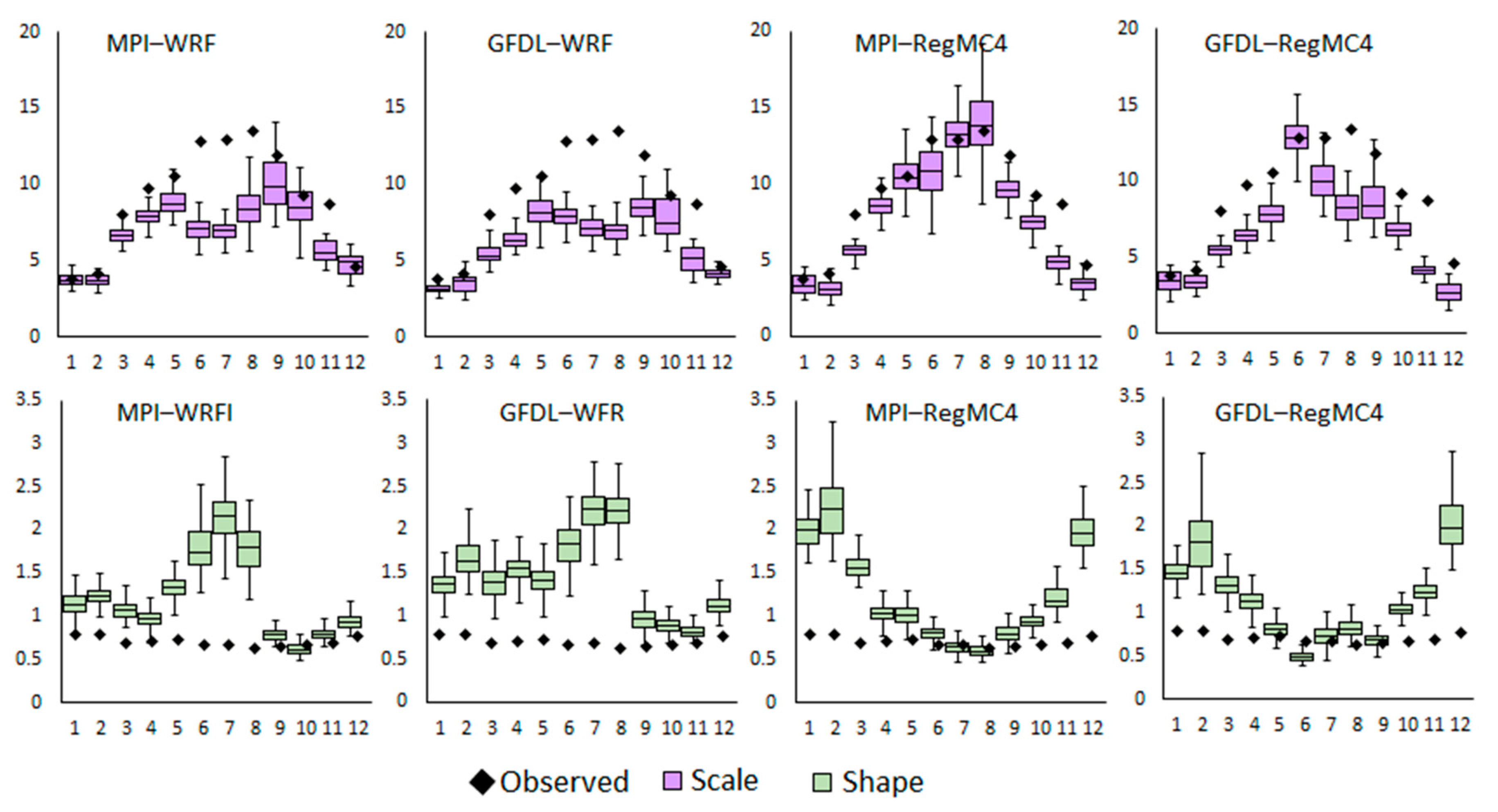
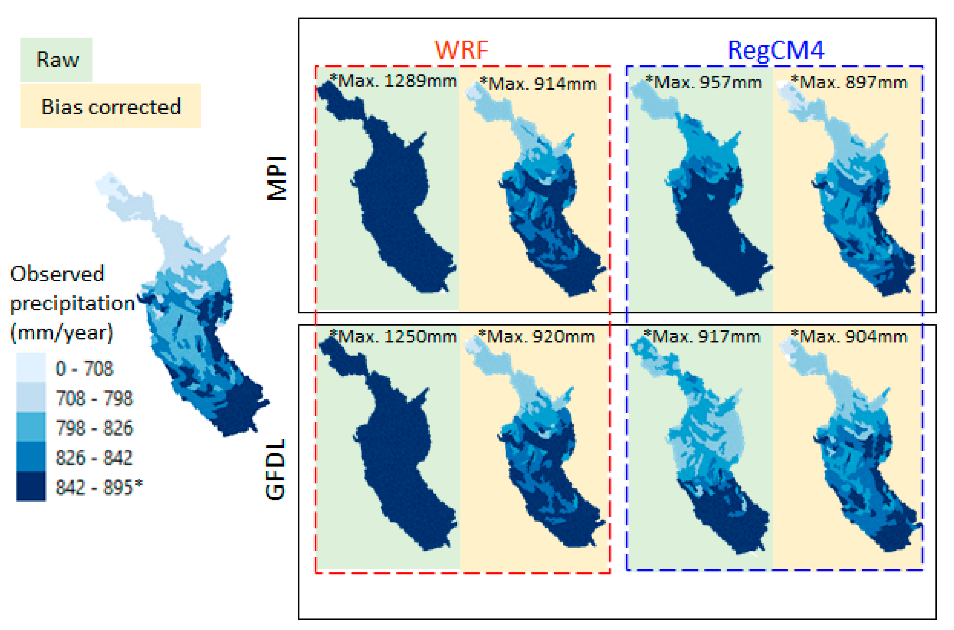
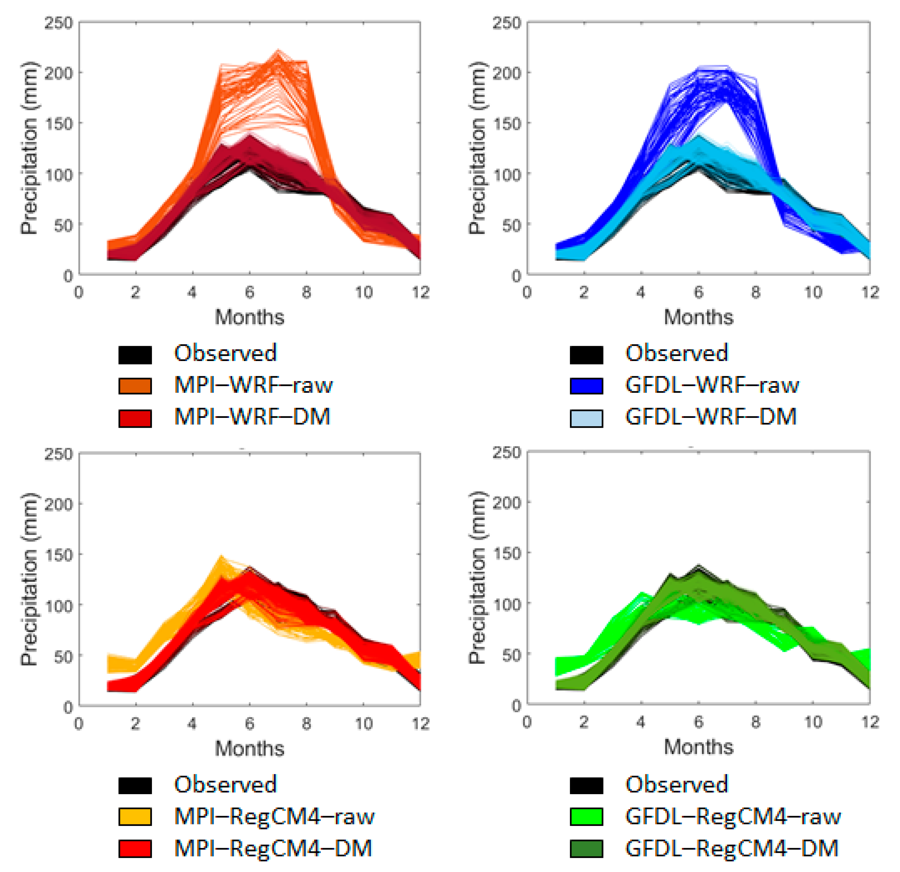
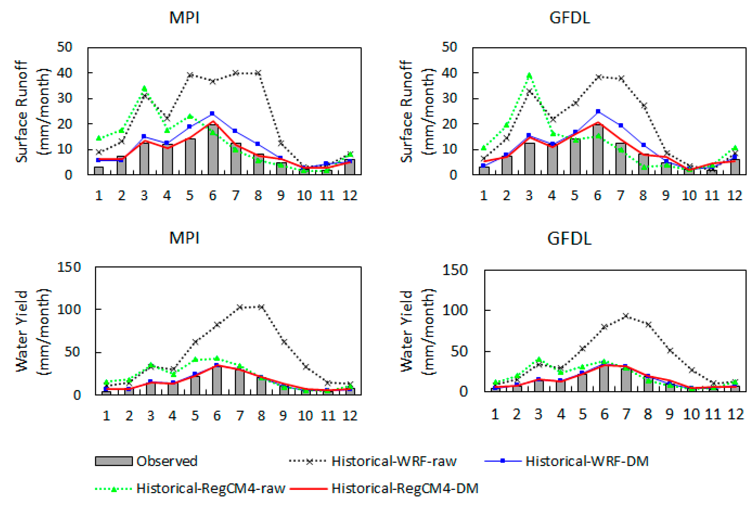
3.1. Historical Precipitation, Surface Runoff, Water Yield, and Streamflow

To understand the effect of bias correction (Distribution Mapping) on GCM-RCM data, we first analyzed the historical run (1981–2005) via precipitation, surface runoff, water yield, and streamflow. The GCM-RCM precipitation products were compared to the PRISM dataset for raw and bias-corrected data. The annual spatial distribution of the precipitation products was compared to the observed data (PRISM) and the time-series seasonal distribution.

Monthly statistical coefficients (RMSE, ME, BIAS, and STDE) were used to evaluate the differences between raw and bias-corrected data (

Table 2. Statistical evaluation for precipitation (monthly) based on four tests: root mean squared error (RMSE), mean error (ME), relative bias (BIAS), and standard deviation (STDE).

	ME (mm)		BIAS (%)		STDE (mm)		RMSE (mm)
	raw	DM	raw	DM	raw	DM	raw	DM
MPI-RegCM4	3.93	−0.14	5.84	−0.21	50.39	55.99	60.33	59.46
MPI-WRF	28.46	1.37	41.97	2.03	84.69	55.35	75.71	58.08
GFDL-RegCM4	0.96	0.26	1.61	0.38	45.77	57.55	59.87	61.06
GFDL-WRF	22.42	1.46	33.11	2.15	75.96	55.48	67.55	57.1

). Overall, the DM models had the best performance, improving the ME and BIAS for all GCM-RCM combinations. The STDE and RMSE were also improved by DM, except for the GFDL-RegCM4 combination.

Figure 3 shows monthly variably of the shape (α) and scale (β) Gamma distribution parameters fitted. The shape parameter average for the observed data is below 1, indicating an exponentially shaped distribution; however, the climate models presented an average fitted distribution greater than 1 in half of the cases, indicating a skewed unimodal distribution curve. When comparing the models, α was better adjusted for RegCM4 combinations. The WRF combination showed better agreement from September to December (with the addition of April for the MPI-WRF combination), and the RegCM4 from April to October. The scale parameter can indicate the probability of extreme events. Smaller values guide to lower probabilities, while larger values imply higher probabilities [21]. The WRF models had a good fit during the winter months; however, the difference is substantial during the rest of the year. The RegCM4 parameters’ distribution showed similar patterns for both models, the MPI-RegCM4 computing the smaller difference between the distributions on average.

Spatial representation of precipitation is still a challenge for applying climate models, even at a ~25-km grid scale. Annual precipitation (1981–2005) for the observed data, raw climate data, and bias-corrected climate data were collated (Figure 4). All eight combinations overestimate annual precipitation; however, the DM strongly reduced historical annual volumes and improved spatial distribution and mean error. Raw WRF models resulted in the most unrealistic precipitation prediction, and the combination MPI-WRF generated the greatest number of volume overestimates. The RegCM4 combination had better agreement with observations for both volume and spatial discretization, as well as for the bias-corrected and raw models.

In addition to spatial variability, an accurate representation of temporal variability (seasonality) is essential, especially to analyze climate change impacts for regional studies. Monthly precipitation was overestimated for all raw models from January to April, and the level of agreement between observed and historical climate projections varied considerably for the two RCM models, with RegCM4 resulting in a better fit (Figure 5). The WRF model’s tendency to overestimate was also apparent at a monthly scale. The WRF model greatly overestimated precipitation from January to August; however, it underestimated precipitation volumes from September to November. In general, the DM bias correction improved monthly precipitation estimates for all GCM-RCM combinations (Figure 5).

The second step of the historical DM data evaluation was conducted using the SWAT model outputs for streamflow, surface runoff, and water yield. Observed streamflow coefficients were compared to the GCM-RCM combinations, accounting for raw and bias-corrected data (Figure 6). The Pbias provides an evaluation of the volumes. The WRF combination for the raw models is outside of the expected ranges for both coefficients; however, an improvement occurs when the DM is applied. The DM improved volume estimations, and after bias correction, all model combinations were within the observed range. The RegCM4 combination also demonstrated reasonable agreement with the raw data.

Initial overprediction and better agreement after the DM was applied also occurred for surface runoff and water yield. More specifically, raw models tended to overpredict surface runoff and water yield, mainly for January to April, and the bias correction provided better agreement for all models, improving their seasonal predictions. After DM application, water yield estimates for MPI/GFDL-WRF and MPI/GFDL-RegCM4 were statistically the same; however, the surface runoff was better represented by the RegCM4 combination (Figure 7). Judging by historical data, the DM method is useful and can overcome various problems (spatial variation, volume estimation, and seasonality) associated with the GCM-RCM model applications. However, good historical representation does not necessarily mean better future prediction. A common use of climate model projections is for future conditions and the corresponding ability to represent hydrological and/or pollutant variables for ecohydrological models such as SWAT (e.g., regional climate change impact studies).

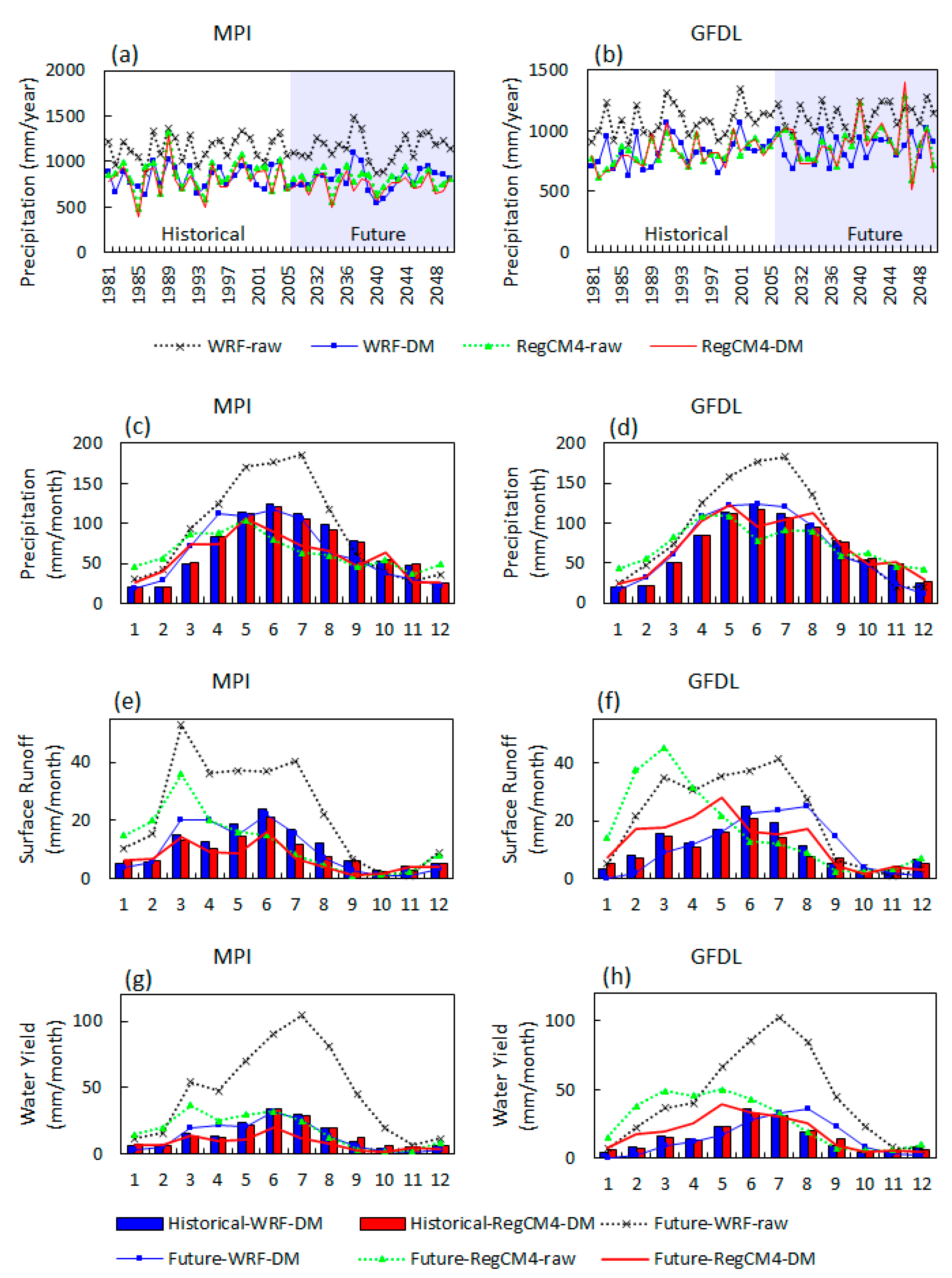
3.2. Future Precipitation, Surface Runoff, and Water Yield

Historical (1981–2005) and future (2030–2049) precipitation, surface runoff, and water yield were compared. Precipitation is presented for both time scales, annual and monthly, and no change in the annual trend was observed, except for the WRF raw model, which estimated an increase of about 35% in annual precipitation volumes (Figure 8a,b). Most model combinations predicted an increase in monthly precipitation from January to March and a reduction for June and July (except for the raw WRF models). In the WRF combination, the precipitation seasonality pattern was maintained with volume reduction from September to December for both raw and bias-corrected simulations. The future scenario estimated by the RegCM4 models showed different seasonal patterns compared to the historical precipitation predictions. The MPI-RegCM4 resulted in a shift from wet to dry months for June to September, and the GFDL-RegCM4 future projection produced the driest conditions for June and September.

SWAT-predicted surface runoff and water yields led to more mixed seasonal patterns than were observed for precipitation, and total volume was overestimated for both variables. The SWAT simulations driven by WRF raw output predicted up to three times greater volume compared to historical runs based on PRISM precipitation data. The SWAT RegCM4-based simulations projected increased surface runoff and water yield for winter and spring by a factor of two and a slight volume reduction in summer and autumn (Figure 8).

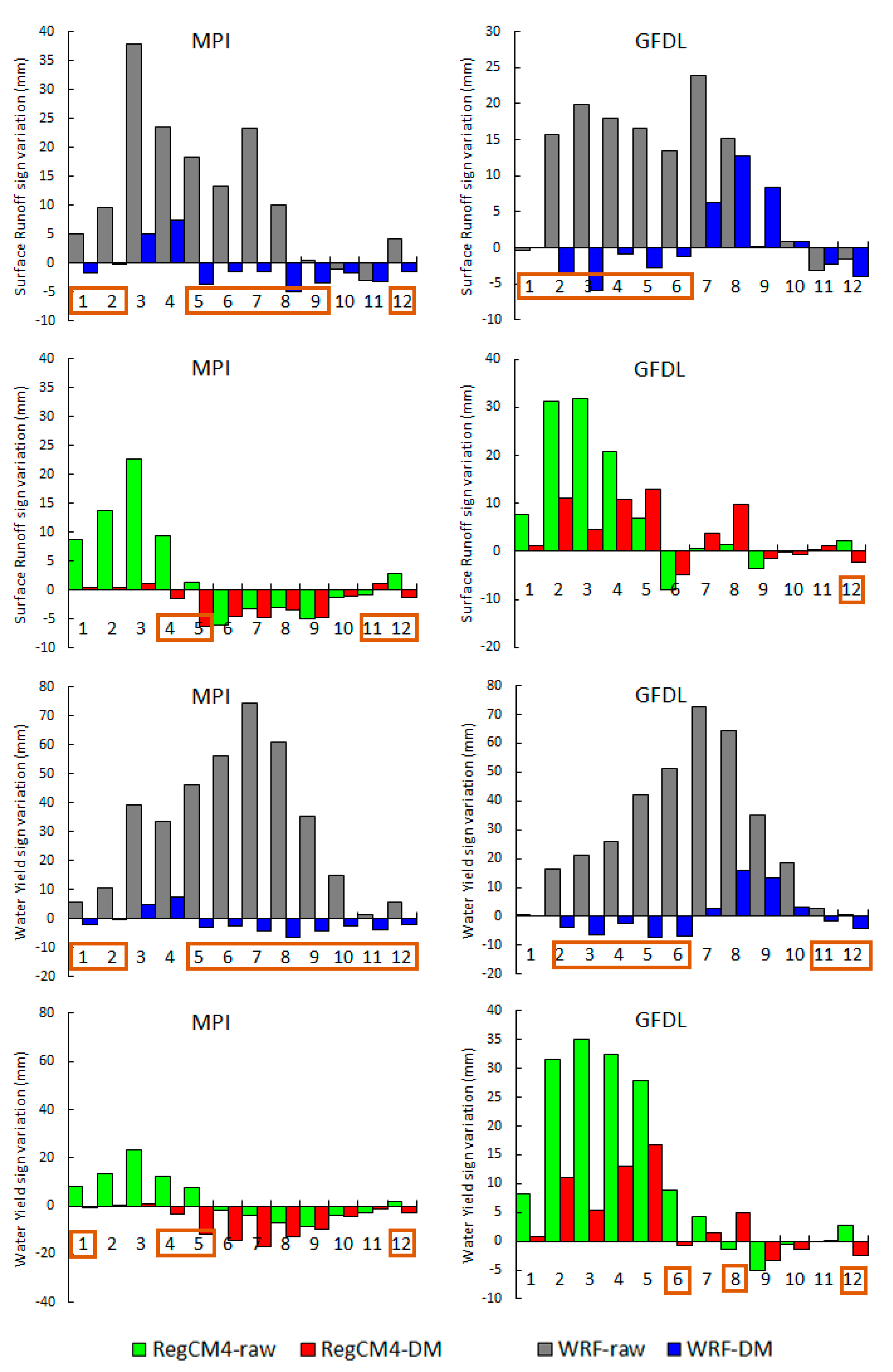
Bias-Correction Models Showed Changes in Prediction Signals

In contrast to the GCM-RCM modeling approaches, bias-correction methods typically have no physical basis; that is, they are not based on the satisfaction of atmospheric conservation laws. That means the bias correction method applied may potentially change the physical relationships between the climate variables and could negatively affect future scenario projections [1,9,14,52]. Future projections (monthly) and changes in prediction signals were calculated by subtracting the historical run values from future scenarios values (Figure 9). If the physical meaning and conservation laws of the model were respected after the DM process, we would expect no difference in volume trends (increases or decreases). However, such changes occurred in some cases.

All model combinations resulted in changes in the prediction signal for at least one of the modeled time periods (months). SWAT simulations executed with the RegCM4 projections showed more consistency in prediction signs, evidenced by the smallest number of months resulting in signal changes for both surface runoff and water yield. However, the SWAT WRF-based combination showed substantial biases and contrary prediction signals in more than 50% of simulated months. The MPI-WRF, for example, led to opposite predictions for each of ten months on average. This outcome suggests the bias correction may be larger than the climate change signal itself and indicates that the procedure is not merely a small correction but a major factor. That also suggests that the representations of physical processes leading to precipitation are so substantially skewed that it casts doubt on their physical realism and how they are responding to changing climate. The limited ability of bias correction has been discussed in previous literature [9,14,52,53,54], suggesting that that process should be viewed with caution if the change signal is smaller than the bias correction. However, this practice is still widely used, and uncertainties are not usually reported or investigated.

Some techniques, such as “quantifying quality” [43] or “model ensemble” [55,56], are available and can mitigate climate scenario uncertainty by assigning weights to the models according to the level of agreement with observations, by sampling all sources of uncertainty along the modeling chain. Models with large biases would receive low weights (and may even be excluded), and models that more accurately replicate observed values receive greater weights [57]. Following this logic, months with the highest predicted uncertainty (those presenting contrary prediction signals, e.g., MPI-WRF January) should receive lower weights or even be excluded from final climate projection analyses.

4. Conclusions

Understanding climate change projections is essential for identifying strategies for adaptation to climate change in response to potential future impacts on important economic sectors such as agriculture. Moreover, bias correction is generally promoted as a necessary step in properly using climate projections for regional studies. Based on SWAT model outputs, we demonstrated how the use of a bias correction method (Distribution Mapping) on precipitation data could shift the valence of hydrological processes on future projections.

In general, we found that: (a) DM improves historical annual and monthly volumes for precipitation and its spatial distribution; (b) monthly precipitation was overestimated for all raw models from January to April (and for the WRF model until August); (c) the ability to detect the occurrence of precipitation events was better for the raw models; (d) simulated historical streamflow was satisfactory for the Pbias coefficient; (e) WRF raw models estimated an increase of about 35% in annual future precipitation; (f) seasonal variability remained the same; (g) increases in monthly precipitation were predicted from January to March, and reductions were predicted for June and July; (h) future surface runoff and water yield were characterized by monthly volume overestimation; and (i) RegCM4 projected increased surface runoff and water yield for winter and spring by a factor of two, and slight volume reductions in summer and autumn.

These findings could help to identify ways to address future climate trends for the region. The change in climate signals that emerged in this study does seem to be an outcome of the bias correction. However, the magnitude of precipitation overprediction in the original projection is concerning. Therefore, the issue (or not) in changing the climate signal points to a problem that may not be the bias correction but the WRF model, for example. The climate signal change does create uncertainty and warrants more research, especially on relevant physical processes, regarding how bias correction is applied for this type of climate projection situation; however, this study underlines issues with the WRF model structure and its extreme overprediction for precipitation data. For future research, we recommend that different bias correction methods be tested. Testing different methods might confirm our findings and could indicate the magnitude of data deviations from RCMs necessary for bias correction methods to be applicable.

References

1. Maraun, D.; Widmann, M.; Gutiérrez, J.M.; Kotlarski, S.; Chandler, R.E.; Hertig, E.; Wibig, J.; Huth, R.; Wilcke, R.A. VALUE: A framework to validate downscaling approaches for climate change studies. Earth’s Futur. 2015, 3, 1–14. [Google Scholar] [CrossRef]
2. Pierce, D.W.; Barnett, T.P.; Santer, B.D.; Gleckler, P.J. Selecting global climate models for regional climate change studies. Proc. Natl. Acad. Sci. USA 2009, 106, 8441–8446. [Google Scholar] [CrossRef]
3. IPCC. Climate Change 2014: Synthesis Report: Longer Report; IPCC: Geneva, Switzerland, 2015. [Google Scholar]
4. Schwalm, C.R.; Glendon, S.; Duffy, P.B. RCP8.5 tracks cumulative CO2 emissions. Proc. Natl. Acad. Sci. USA 2020, 117, 19656–19657. [Google Scholar] [CrossRef] [PubMed]
5. Pinto, I.; Jack, C.; Hewitson, B. Process-based model evaluation and projections over southern Africa from Coordinated Regional Climate Downscaling Experiment and Coupled Model Intercomparison Project Phase 5 models. Int. J. Clim. 2018, 38, 4251–4261. [Google Scholar] [CrossRef]
6. Arnold, J.G.; Srinivasan, R.; Muttiah, R.S.; Williams, J.R. LARGE AREA HYDROLOGIC MODELING AND ASSESSMENT PART I: MODEL DEVELOPMENT. JAWRA J. Am. Water Resour. Assoc. 1998, 34, 73–89. [Google Scholar] [CrossRef]
7. Williams, J.R.; Arnold, J.G.; Kiniry, J.R.; Gassman, P.W.; Green, C.H. History of model development at Temple, Texas. Hydrol. Sci. J. 2008, 53, 948–960. [Google Scholar] [CrossRef]
8. Bieger, K.; Arnold, J.G.; Rathjens, H.; White, M.J.; Bosch, D.D.; Allen, P.M.; Volk, M.; Srinivasan, R. Introduction to SWAT+, A Completely Restructured Version of the Soil and Water Assessment Tool. JAWRA J. Am. Water Resour. Assoc. 2016, 53, 115–130. [Google Scholar] [CrossRef]
9. Ehret, U.; Zehe, E.; Wulfmeyer, V.; Warrach-Sagi, K.; Liebert, J. HESS Opinions "Should we apply bias correction to global and regional climate model data?". Hydrol. Earth Syst. Sci. 2012, 16, 3391–3404. [Google Scholar] [CrossRef]
10. Sørland, S.L.; Schär, C.; Luethi, D.; Kjellström, E. Bias patterns and climate change signals in GCM-RCM model chains. Environ. Res. Lett. 2018, 13, 074017. [Google Scholar] [CrossRef]
11. Teutschbein, C.; Seibert, J. Is bias correction of regional climate model (RCM) simulations possible for non-stationary conditions? Hydrol. Earth Syst. Sci. 2013, 17, 5061–5077. [Google Scholar] [CrossRef] [Green Version]
12. Singh, V.; Jain, S.K.; Singh, P. Inter-comparisons and applicability of CMIP5 GCMs, RCMs and statistically downscaled NEX-GDDP based precipitation in India. Sci. Total. Environ. 2019, 697, 134163. [Google Scholar] [CrossRef] [PubMed]
13. Stéfanon, M.; Martin-StPaul, N.K.; Leadley, P.; Bastin, S.; Dell’Aquila, A.; Drobinski, P.; Gallardo, C. Testing climate models using an impact model: What are the advantages? Clim. Chang. 2015, 131, 649–661. [Google Scholar] [CrossRef]
14. Wörner, V.; Kreye, P.; Meon, G. Effects of Bias-Correcting Climate Model Data on the Projection of Future Changes in High Flows. Hydrology 2019, 6, 46. [Google Scholar] [CrossRef]
15. Bathurst, J.; Ewen, J.; Parkin, G.; O’Connell, P.; Cooper, J. Validation of catchment models for predicting land-use and climate change impacts. Blind validation for internal and outlet responses. J. Hydrol. 2004, 287, 74–94. [Google Scholar] [CrossRef]
16. Kundu, S.; Khare, D.; Mondal, A. Individual and combined impacts of future climate and land use changes on the water balance. Ecol. Eng. 2017, 105, 42–57. [Google Scholar] [CrossRef]
17. Pandey, B.K.; Khare, D.; Kawasaki, A.; Meshesha, T.W. Integrated approach to simulate hydrological responses to land use dynamics and climate change scenarios employing scoring method in upper Narmada basin, India. J. Hydrol. 2021, 598, 126429. [Google Scholar] [CrossRef]
18. Chagas, V.B.P.; Chaffe, P.L.B.; Blöschl, G. Climate and land management accelerate the Brazilian water cycle. Nat. Commun. 2022, 13, 5136. [Google Scholar] [CrossRef] [PubMed]
19. Iowa Climate Statement 2013: A Rising Challenge to Iowa Agriculture. Available online: https://cgrer.uiowa.edu/sites/cgrer.uiowa.edu/files/pdf_files/Iowa%20Climate%20Statement%202013%20A%20Rising%20Challenge%20to%20Iowa%20Agriculture_October_18_2013_FINAL.pdf (accessed on 5 January 2023).
20. Iowa Climate Statement 2019: Dangerous Heat Events Will Be More Frequent and Severe. Available online: http://www.craiganderson.org/wp-content/uploads/caa/ClimateChangeDocs/2019IowaClimateStatement.pdf (accessed on 5 January 2023).
21. Teutschbein, C.; Seibert, J. Bias correction of regional climate model simulations for hydrological climate-change impact studies: Review and evaluation of different methods. J. Hydrol. 2012, 456–457, 12–29. [Google Scholar] [CrossRef]
22. Beven, K.; Lamb, R. The uncertainty cascade in model fusion. Geol. Soc. London Spéc. Publ. 2014, 408, 255–266. [Google Scholar] [CrossRef]
23. Clark, M.P.; Wilby, R.L.; Gutmann, E.D.; Vano, J.A.; Gangopadhyay, S.; Wood, A.W.; Fowler, H.J.; Prudhomme, C.; Arnold, J.R.; Brekke, L.D. Characterizing Uncertainty of the Hydrologic Impacts of Climate Change. Curr. Clim. Chang. Rep. 2016, 2, 55–64. [Google Scholar] [CrossRef] [Green Version]
24. Brighenti, T.M.; Gassman, P.W.; Schilling, K.E.; Srinivasan, R.; Liebman, M.; Thompson, J.R. Determination of accurate baseline representation for three Central Iowa watersheds within a HAWQS-based SWAT analyses. Sci. Total. Environ. 2022, 839, 156302. [Google Scholar] [CrossRef]
25. Gassman, P.; Reyes, M.; Green, C.; Arnold, J.; Gassman, P. The Soil And Water Assessment Tool: Historical Development, Applications, and Future Research Directions Invited Review Series. Trans. ASABE 2007, 50, 1211–1250. [Google Scholar] [CrossRef]
26. Tan, M.L.; Gassman, P.W.; Yang, X.; Haywood, J. A review of SWAT applications, performance and future needs for simulation of hydro-climatic extremes. Adv. Water Resour. 2020, 143, 103662. [Google Scholar] [CrossRef]
27. Akoko, G.; Le, T.; Gomi, T.; Kato, T. A Review of SWAT Model Application in Africa. Water 2021, 13, 1313. [Google Scholar] [CrossRef]
28. USDA-NRCS (U.S. Department of Agriculture, Natural Resources Conservation Service). Soil Data Access: Query Services for Custom Access to Soil Data; USDA-NRCS: Washington, DC, USA. Available online: https://sdmdataaccess.nrcs.usda.gov/ (accessed on 5 January 2023).
29. Peel, M.; Finlayson, B.; Mcmahon, T. Hydrology and Earth System Sciences Updated World Map of the Köppen-Geiger Climate Classification. 2007. Available online: www.hydrol-earth-syst-sci.net/11/1633/2007/ (accessed on 5 January 2023).
30. McGinnis, S.; Mearns, L. Building a climate service for North America based on the NA-CORDEX data archive. Clim. Serv. 2021, 22, 100233. [Google Scholar] [CrossRef]
31. PRISM (Parameter-Elevation Relationships on Independent Slopes Model). Climate Group, PRISM Climate Data, Northwest Alliance for Computational Science and Engineering; Oregon State University: Corvallis, OR, USA; Available online: https://www.prism.oregonstate.edu/ (accessed on 5 January 2023).
32. USGS National Water Information System, Streamflow Data Access. 2021. Available online: https://waterdata.usgs.gov/nwis (accessed on 5 January 2023).
33. WRCP (World Climate Research Programme). CMIP Phase 5 (CMIP5); World Meteorological Organization: Geneva, Switzerland; Available online: https://www.wcrp-climate.org/wgcm-cmip/wgcm-cmip5 (accessed on 5 January 2023).
34. Giorgi, F.; Jones, C.; Asrar, G. Addressing Climate Information Needs at the Regional Level: The CORDEX Framework. 2009. Available online: http://wcrp.ipsl (accessed on 5 January 2023).
35. CORDEX Simulations Summary. Summary of Regional Climate Change Simulations Available for the CORDEX Domains. Available online: https://cordex.org/wp-content/uploads/2020/12/Summary_CORDEX_simulations_Nov_2020.pdf (accessed on 5 January 2023).
36. NCAR (National Center for Atmospheric Research). NA-CORDEX Simulation Matrix. The North American CORDEX Program; NCAR Climate Data Gateway: Boulder, CO, USA; Available online: https://na-cordex.org/simulation-matrix.html (accessed on 5 January 2023).
37. Giorgi, F.; Coppola, E.; Solmon, F.; Mariotti, L.; Sylla, M.B.; Bi, X.; Elguindi, N.; Diro, G.T.; Nair, V.; Giuliani, G.; et al. RegCM4: Model description and preliminary tests over multiple CORDEX domains. Clim. Res. 2012, 52, 7–29. [Google Scholar] [CrossRef]
38. Brighenti, T.M.; Bonumá, N.B.; Srinivasan, R.; Chaffe, P.L.B. Simulating sub-daily hydrological process with SWAT: A review. Hydrol. Sci. J. 2019, 64, 1415–1423. [Google Scholar] [CrossRef]
39. Neitsch, S.; Arnold, J.; Kiniry, J.; Williams, J. College Of Agriculture And Life Sciences Soil and Water Assessment Tool Theoretical Documentation Version 2009; Texas Water Resources Institute: College Station, TX, USA, 2011. [Google Scholar]
40. Arnold, J.; Moriasi, D.; Gassman, P.; Abbaspour, K.; White, M.; Srinivasan, R.; Santhi, C.; Harmel, R.; van Griensven, A.; van Liew, M.; et al. SWAT: Model Use, Calibration, and Validation. Trans. ASABE 2012, 55, 1491–1508. Available online: http://swatmodel.tamu.edu (accessed on 5 January 2023). [CrossRef]
41. Rathjens, H.; Bieger, K.; Srinivasan, R.; Arnold, J. CMhyd User Manual. Documentation for Preparing Simulated Climate Change Data for Hydrologic Impact Studies. 2016. Available online: https://swat.tamu.edu/media/115265/bias_cor_man.pdf (accessed on 5 January 2023).
42. Sangelantoni, L.; Tomassetti, B.; Colaiuda, V.; Lombardi, A.; Verdecchia, M.; Ferretti, R.; Redaelli, G. On the Use of Original and Bias-Corrected Climate Simulations in Regional-Scale Hydrological Scenarios in the Mediterranean Basin. Atmosphere 2019, 10, 799. [Google Scholar] [CrossRef]
43. de Amorim, P.B.; Chaffe, P.B. Towards a comprehensive characterization of evidence in synthesis assessments: The climate change impacts on the Brazilian water resources. Clim. Chang. 2019, 155, 37–57. [Google Scholar] [CrossRef]
44. Maraun, D. Bias Correction, Quantile Mapping, and Downscaling: Revisiting the Inflation Issue. J. Clim. 2013, 26, 2137–2143. [Google Scholar] [CrossRef]
45. Sangelantoni, L.; Russo, A.; Gennaretti, F. Impact of bias correction and downscaling through quantile mapping on simulated climate change signal: A case study over Central Italy. Theor. Appl. Clim. 2018, 135, 725–740. [Google Scholar] [CrossRef]
46. USGS Hydrologic Unit Codes (HUCs) Explained. Available online: https://nas.er.usgs.gov/hucs.aspx (accessed on 5 January 2023).
47. Hodson, T.O. Root-mean-square error (RMSE) or mean absolute error (MAE): When to use them or not. Geosci. Model Dev. 2022, 15, 5481–5487. [Google Scholar] [CrossRef]
48. Jackson, E.K.; Roberts, W.; Nelsen, B.; Williams, G.P.; Nelson, E.J.; Ames, D.P. Introductory overview: Error metrics for hydrologic modelling—A review of common practices and an open source library to facilitate use and adoption. Environ. Model. Softw. 2019, 119, 32–48. [Google Scholar] [CrossRef]
49. Meng, J.; Li, L.; Hao, Z.; Wang, J.; Shao, Q. Suitability of TRMM satellite rainfall in driving a distributed hydrological model in the source region of Yellow River. J. Hydrol. 2014, 509, 320–332. [Google Scholar] [CrossRef]
50. Moriasi, D.N.; Gitau, M.W.; Pai, N.; Daggupati, P. Hydrologic and Water Quality Models: Performance Measures and Evaluation Criteria. Trans. ASABE 2015, 58, 1763–1785. [Google Scholar] [CrossRef]
51. Moriasi, D.; Arnold, J.; van Liew, M.; Bingner, R.; Harmel, R.; Veith, T. Model Evaluation Guidelines For Systematic Quantification of Accuracy in Watershed Simulations. Trans. ASABE 1983, 50, 885–900. [Google Scholar] [CrossRef]
52. Maraun, D. Bias Correcting Climate Change Simulations—A Critical Review. Curr. Clim. Chang. Rep. 2016, 2, 211–220. [Google Scholar] [CrossRef]
53. Muerth, M.J.; Gauvin St-Denis, B.; Ricard, S.; Velázquez, J.A.; Schmid, J.; Minville, M.; Caya, D.; Chaumont, D.; Ludwig, R.; Turcotte, R. On the need for bias correction in regional climate scenarios to assess climate change impacts on river runoff. Hydrol. Earth Syst. Sci. 2013, 17, 1189–1204. [Google Scholar] [CrossRef]
54. Maraun, D.; Shepherd, T.G.; Widmann, M.; Zappa, G.; Walton, D.; Gutiérrez, J.M.; Hagemann, S.; Richter, I.; Soares, P.M.; Hall, A.; et al. Towards process-informed bias correction of climate change simulations. Nat. Clim. Change 2017, 7, 764–773. [Google Scholar] [CrossRef] [Green Version]
55. Padrón, R.S.; Gudmundsson, L.; Seneviratne, S.I. Observational Constraints Reduce Likelihood of Extreme Changes in Multidecadal Land Water Availability. Geophys. Res. Lett. 2019, 46, 736–744. [Google Scholar] [CrossRef] [PubMed]
56. Herger, N.; Abramowitz, G.; Sherwood, S.; Knutti, R.; Angélil, O.; Sisson, S.A. Ensemble optimisation, multiple constraints and overconfidence: A case study with future Australian precipitation change. Clim. Dyn. 2019, 53, 1581–1596. [Google Scholar] [CrossRef]
57. Sanderson, B.M.; Knutti, R. On the interpretation of constrained climate model ensembles. Geophys. Res. Lett. 2012, 39, 2012gl052665. [Google Scholar] [CrossRef] [Green Version]
Figure 1. Locations of the Des Moines River Basin in Iowa and Minnesota, USA, the Des Moines Metropolitan Statistical Area, and streamflow monitoring stations.
Water 15 00750 g001
Figure 2. Methodological framework for assessing the influence of applying bias correction (distribution mapping for precipitation data) to future climate scenarios and using the SWAT model to evaluate the impacts.
Water 15 00750 g002
Figure 3. Variability (monthly) of shape and scale parameters (boxplot) of the Gamma distribution for the historical run during the bias-correction process, the black diamond represents the average parameter values for observed precipitation.
Water 15 00750 g003
Figure 4. Spatial representation of observed annual precipitation (1981–2005), raw climate data, and bias-corrected climate data. The * refers to the replacement of the maximum rainfall value (in the legend) for each model.
Water 15 00750 g004
Figure 5. Seasonal representation of precipitation (1981–2005) for observed data, raw climate data, and bias-corrected climate data.
Water 15 00750 g005
Figure 6. Streamflow Pbias coefficient of the historical period; boxplots for observed data, raw climate data, and bias-corrected climate data. The yellow band is a visual extension of the observed results to help visualize the target range of values.
Water 15 00750 g006
Figure 7. Monthly surface runoff and water yield outputs for observed data, raw climate data, and bias-corrected climate data for the 1981 to 2005 time period.
Water 15 00750 g007
Figure 8. Comparisons for raw and bias-corrected data for historical (1981–2005) and future (2030–2049) precipitation, surface runoff, and water yield. Each shows the result of a GCM-RCM combination: Precipitation is presented for annual and monthly scales (ad), and surface runoff and water yield at a monthly time-step (eh).
Water 15 00750 g008
Figure 9. Representation of monthly future projections and changes in prediction signals for surface runoff and water yield. Each figure shows a GCM-RCM combination of raw and bias-corrected data; the orange squares indicate months where changes in prediction signal occur.
Water 15 00750 g009