
Comparing the Runoff Decompositions of Small Experimental Catchments: End-Member Mixing Analysis (EMMA) vs. Hydrological Modelling
 , ,
, ,  , and
, and
Abstract
:1. Introduction
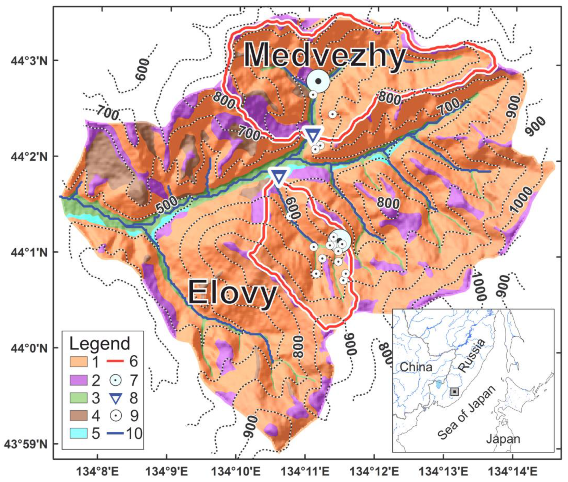
2. Description of Study Objects, Data, and Measurements Methods
2.1. EMMA Model
2.2. ECOMAG Model
2.3. SWAT Model
2.4. HBV Model
3. Results
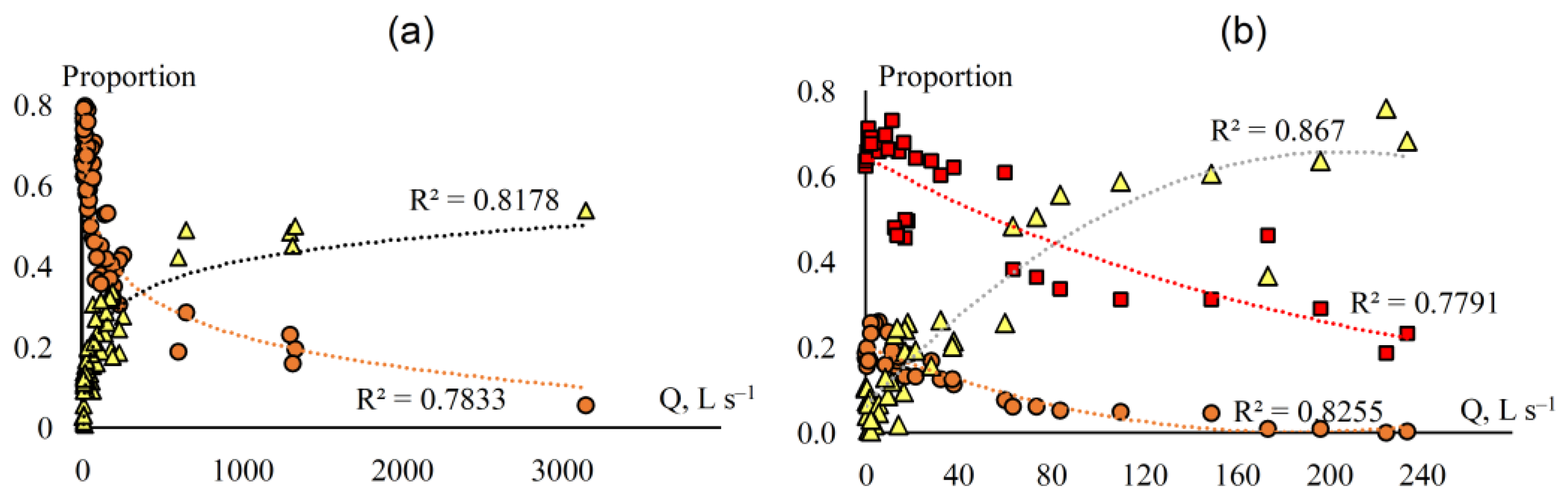
3.1. EMMA Results
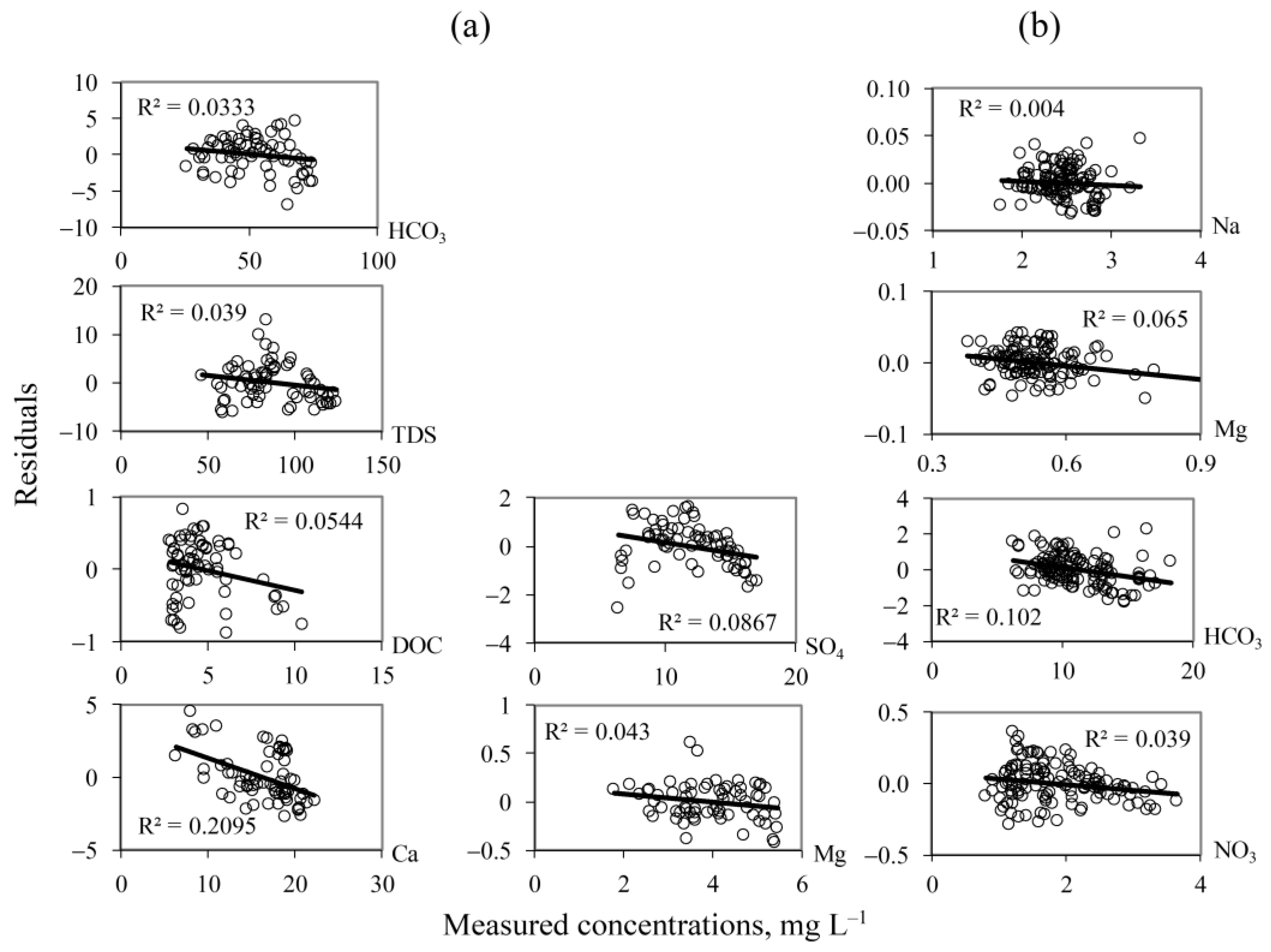
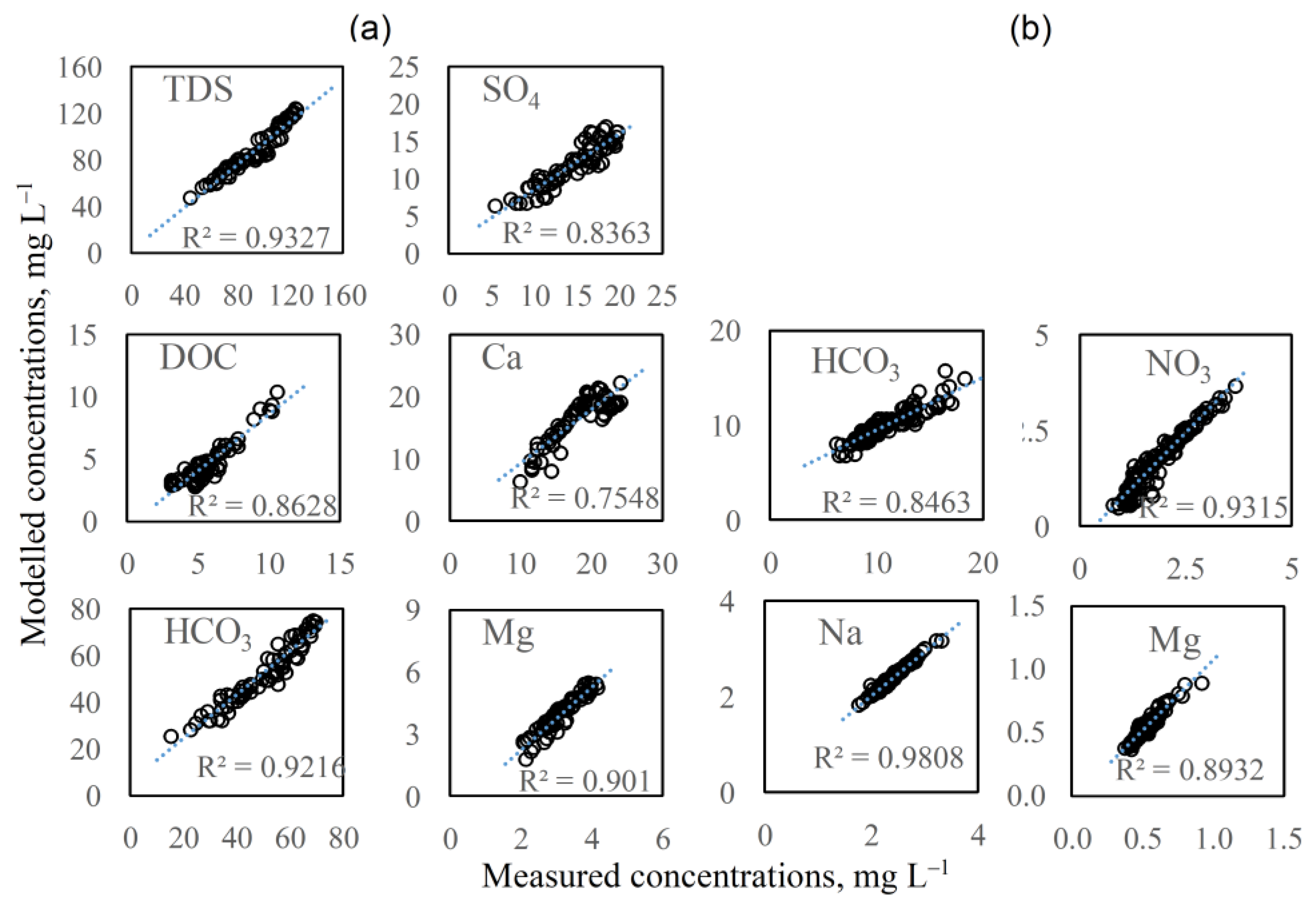
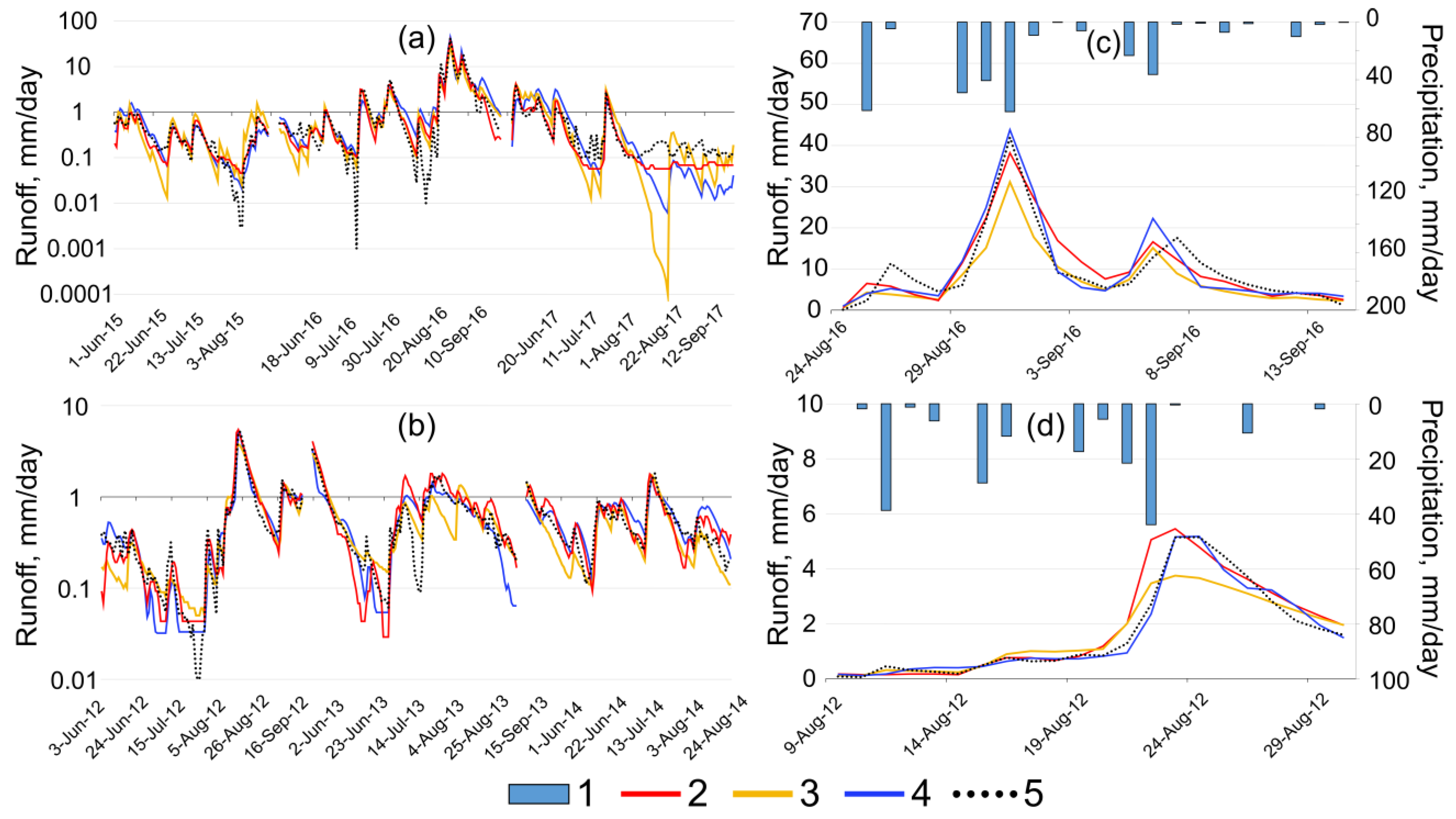
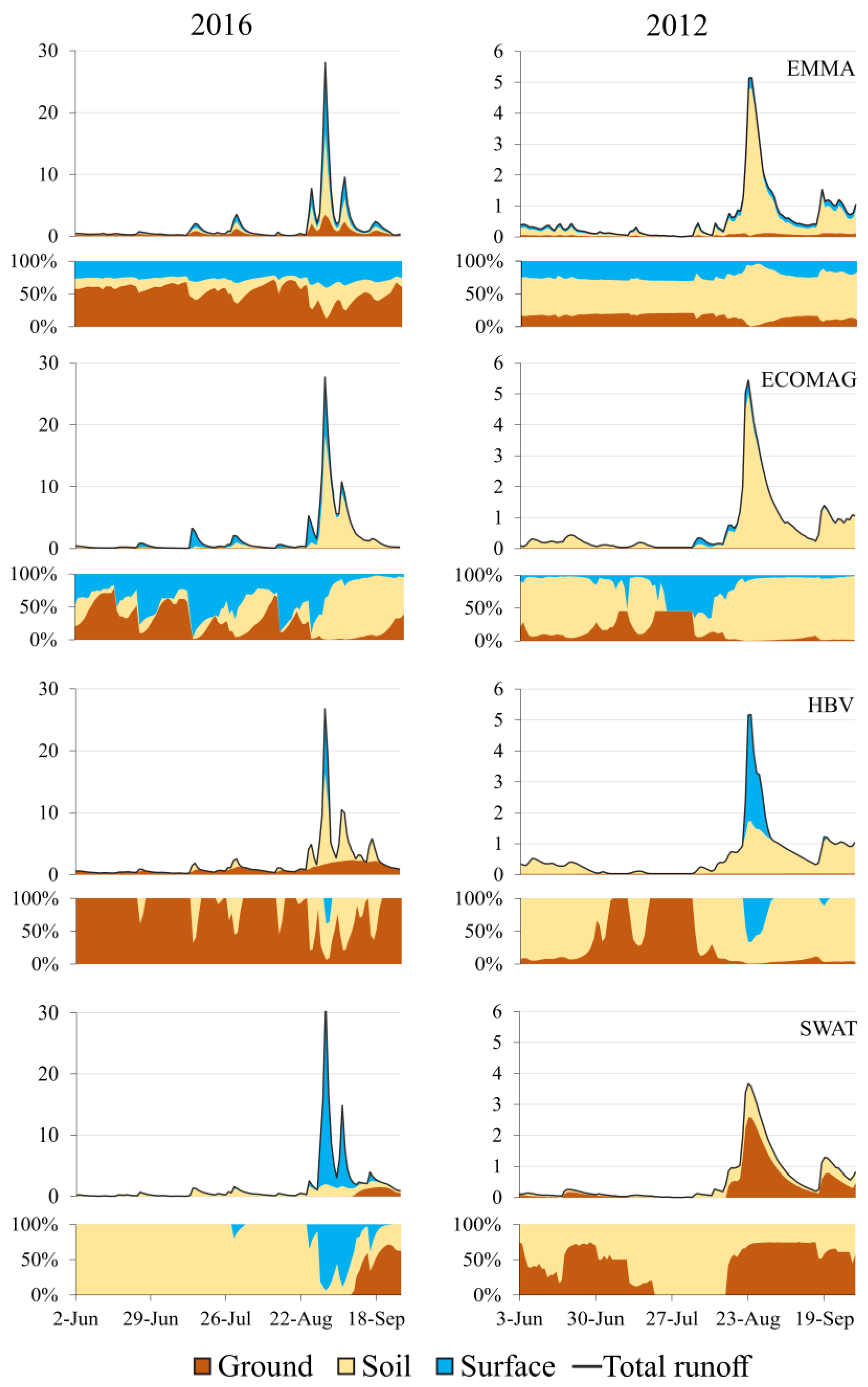
3.2. Results of Hydrological Simulations
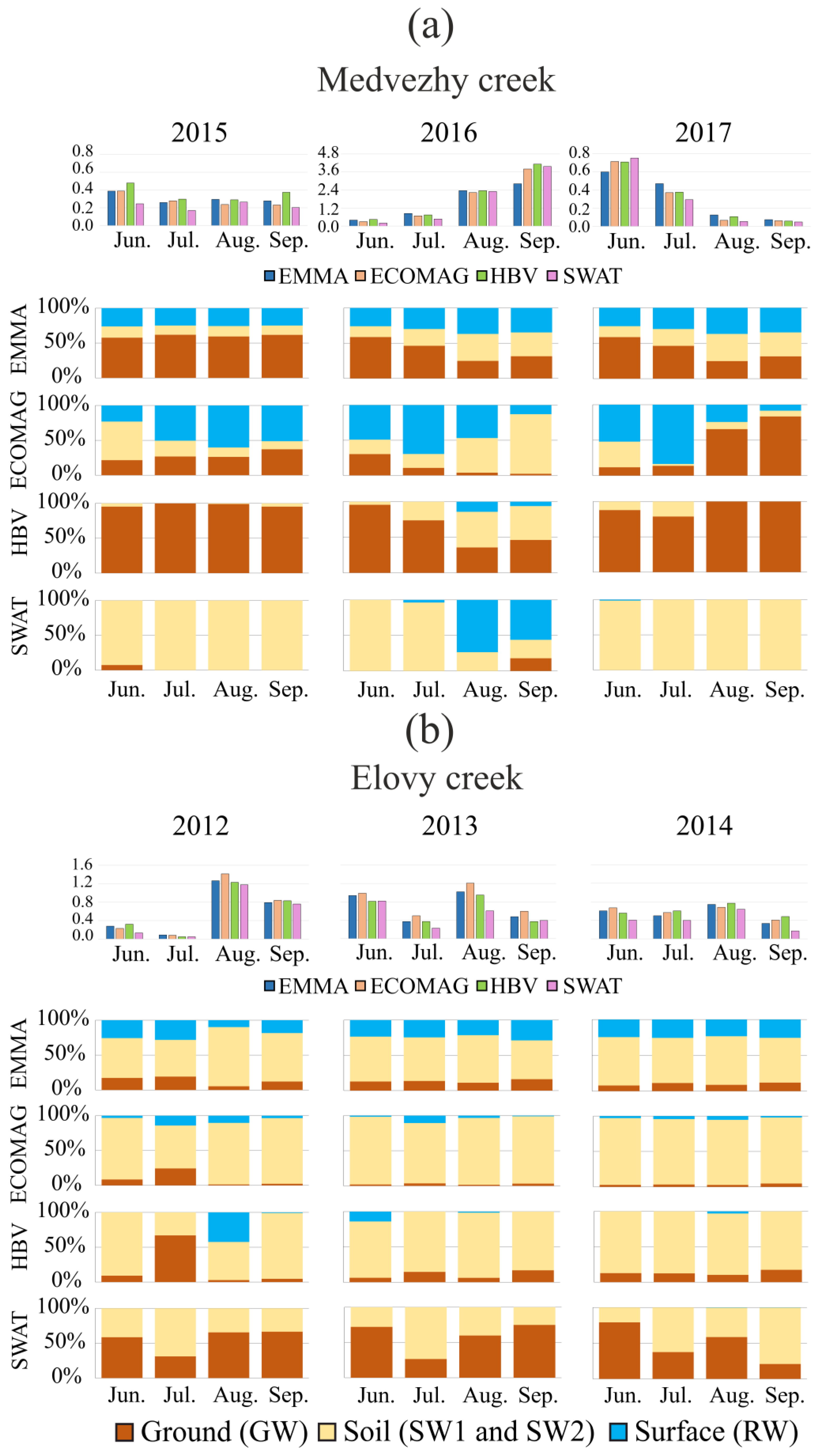
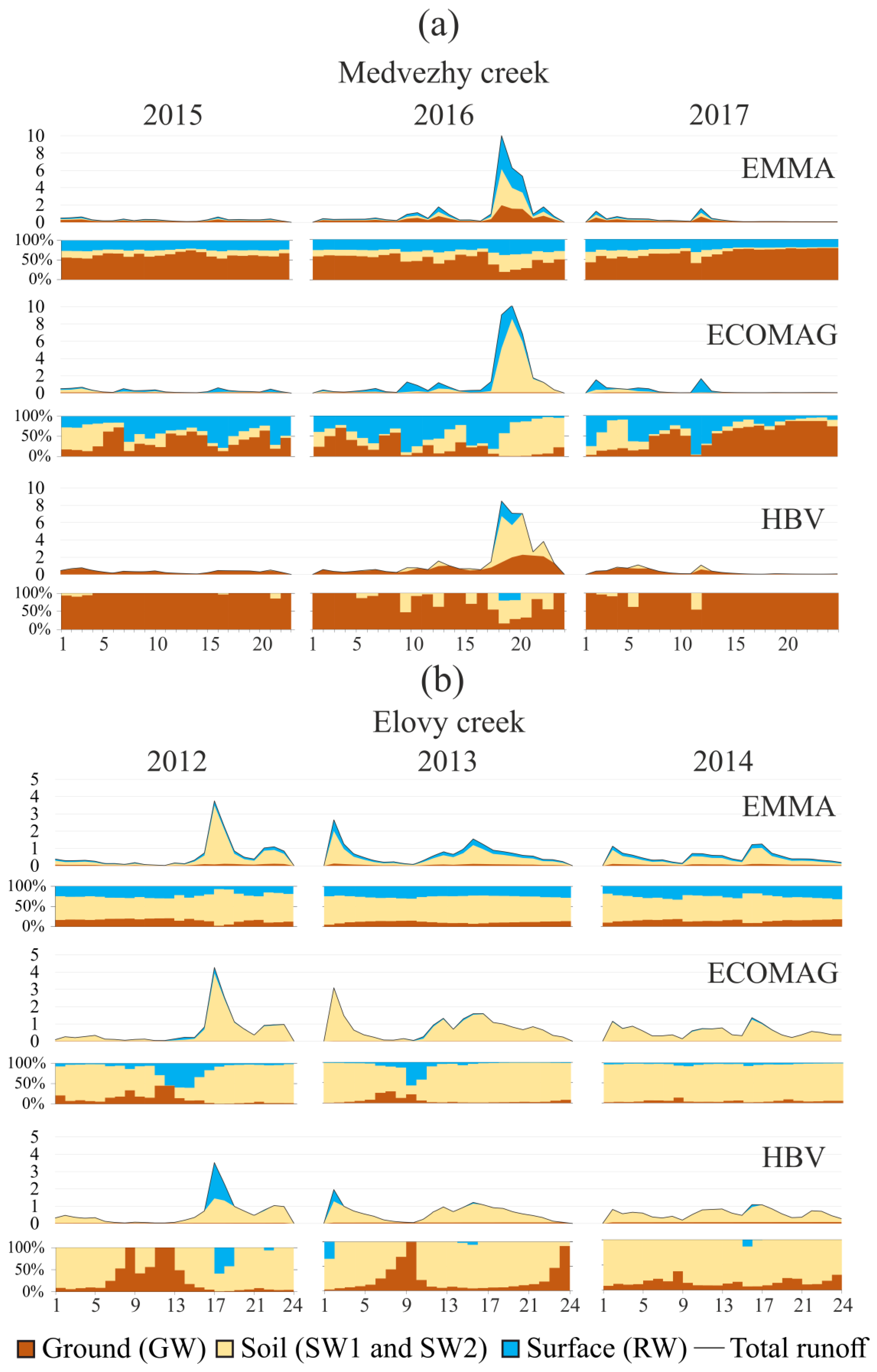
4. Discussion of Hydrograph Separations
5. Conclusions
Author Contributions
Funding
Data Availability Statement
Conflicts of Interest
Appendix A

| Parameter | Short Name | Medvezhy | Elovy |
|---|---|---|---|
| Coef. of vertical saturated hydraulic conductivity | GFB | 8.3 | 6.5 |
| Coef. of horizontal saturated hydraulic conductivity | GFA | 1 | 10 |
| Soil evaporation coefficient | EK | 0.75 | 0.8 |
| Baseflow constant, mm day−1 | GROUND | 0.009 | 0.0001 |
| Coef. of snowmelt intensity, mm day−1 °C | ALF | 0.28 | 0.45 |
| Critical air temperature snow/rain, °C | TCR | 0.5 | 0.5 |
| Snowmelt air temperature, °C | TSN | 0.1 | 0.1 |
| Air temperature gradient, °C 100 m−1 | TGR | −0.6 | −0.6 |
| Precipitation gradient, mm 100 m−1 | PGR | 0 | 0 |
| Coef. of vertical saturated hydraulic conductivity | GFB | 8.3 | 6.5 |
| Coef. of horizontal saturated hydraulic conductivity | GFA | 1 | 10 |
Appendix B
| Parameter | Short Name | Medvezhy | Elovy |
|---|---|---|---|
| SCS runoff curve number for moisture condition II | CN2 | 35.0 | 35.0 |
| Roughness coefficient for overland flow | OV_N | 30.0 | 0.01 |
| Evaporation compensation from soil | ESCO | 0.1 | 0.46 |
| Travel time of lateral flow, days | LAT_TTIME | 3.5 | 7.7 |
| Depth of the impervious layer, m | DEP_IMP | 4.25 | 5.1 |
| Baseflow recession constant | ALPHA_BF | 0.25 | 0.13 |
| Time to reach the groundwater, days | GW_DELAY | 1.5 | 1.55 |
| Recharge of deep aquifer coefficient | RCHRG_DP | 0.55 | 0.24 |
| Threshold for return flow to occur, mm | GWQMN | 50 | 0.0 |
| Capillary rise coefficient | GW_REVAP | 0.2 | 0.2 |
| Threshold for GW_REVAP to occur, mm | REVAPMN | 25 | 0 |
| Slope length for lateral subsurface flow, m | SLSOIL | 48 | 59 |
Appendix C
| Parameter | Short Name | Medvezhy | Elovy |
|---|---|---|---|
| Max. soil storage content, mm | FC | 350 | 150 |
| PET limit | LP | 0.2 | 0.58 |
| Recharge parameter | Beta | 1.7 | 2.7 |
| Max. percolation rate, mm day−1 | PERC | 2.6 | 1.6 |
| Upper zone limit, mm | HL | 28 | 45 |
| Recession coef. | K0 | 0.99 | 0.16 |
| Recession coef. | K1 | 0.40 | 0.03 |
| Recession coef. | K2 | 0.13 | 0.0001 |
| Length of triangular weighting function, days | MAXBAS | 1.8 | 2.9 |
| PET correction factor, 1 °C−1 | Cet | 0 | 0.03 |
References
- Heidbüchel, I.; Troch, P.A.; Lyon, S.W.; Weiler, M. The master transit time distribution of variable flow systems. Water Resour. Res. 2012, 48, W06520. [Google Scholar] [CrossRef]
- Perrin, C.; Michel, C.; Andreassian, V. Improvement of a Parsimonious Model for Streamflow Simulation. J. Hydrol. 2003, 279, 275–289. [Google Scholar] [CrossRef]
- Gartsman, B.I.; Shamov, V.V. Field studies of runoff formation in the Far East region based on modern observational instruments. Water Resour. 2015, 42, 766–775. [Google Scholar] [CrossRef]
- Cerda, A.; Novara, A.; Dlapa, P.; Lopez-Vicente, M.; Ubeda, X.; Popovic, Z.; Mekonnen, M.; Terol, E.; Janizadeh, S.; Mbarki, S.; et al. Rainfall and water yield in Macizo del Caroig, Eastern Iberian Peninsula. Event runoff at plot scale during a rare flash flood at the Barranco de Benacancil. Cuad. Investig. Geografica 2021, 47, 95–119. [Google Scholar] [CrossRef]
- Széles, B.; Parajka, J.; Hogan, P.; Silasari, R.; Pavlin, L.; Strauss, P.; Blöschl, G. The added value of different data types for calibrating and testing a hydrologic model in a small catchment. Water Resour. Res. 2020, 56, e2019WR026153. [Google Scholar] [CrossRef] [PubMed]
- Dunn, S.M.; Freer, J.E.; Weiler, M.; Kirkby, M.J.; Seibert, J.; Quinn, P.F.; Lischeid, G.; Tetzlaff, D.; Soulsby, C. Conceptualization in catchment modeling: Simply learning? Hydrol. Process. 2008, 22, 2389–2393. [Google Scholar] [CrossRef]
- Johnson, M.S.; Coon, W.F.; Mehta, V.K.; Steenhuis, T.S.; Brooks, E.S.; Boll, J. Application of two hydrologic models with different runoff mechanisms to a hillslope dominated watershed in the northeastern US: A comparison of HSPF and SMR. J. Hydrol. 2003, 284, 57–76. [Google Scholar] [CrossRef]
- Butts, M.B.; Payne, J.T.; Kristensen, M.; Madsen, H. An evaluation of the impact of model structure on hydrological modeling uncertainty for streamflow simulation. J. Hydrol. 2004, 298, 242–266. [Google Scholar] [CrossRef]
- Clark, M.P.; Slater, A.G.; Rupp, D.E.; Woods, R.A.; Vrugt, J.A.; Gupta, H.V.; Wagener, T.; Hay, L.E. Framework for Understanding Structural Errors (FUSE): A modular framework to diagnose differences between hydrological models. Water Resour. Res. 2008, 44, W00B02. [Google Scholar] [CrossRef]
- Clark, M.P.; Kavetski, D.; Fenicia, F. Pursuing the method of multiple working hypotheses for hydrological modelling. Water Resour. Res. 2011, 47, W09301. [Google Scholar] [CrossRef] [Green Version]
- Li, H.; Xu, C.-Y.; Beldring, S. How much can we gain with increasing model complexity with the same model concepts? J. Hydrol. 2015, 527, 858–871. [Google Scholar] [CrossRef]
- Atkinson, S.E.; Woods, R.A.; Sivapalan, M. Climate and landscape controls on water balance model complexity over changing landscapes. Water Resour. Res. 2002, 38, 1314. [Google Scholar] [CrossRef]
- Sivapalan, M.; Blöschl, G.; Zhang, L.; Vertessy, R. Downward approach to hydrological prediction. Hydrol. Process. 2003, 17, 2101–2111. [Google Scholar] [CrossRef]
- Marshall, L.; Sharma, A.; Nott, D. Modeling the catchment via mixtures: Issues of model specification and validation. Water Resour. Res. 2006, 42, W11409. [Google Scholar] [CrossRef]
- Bai, Y.; Wagener, T.; Reed, P. A top-down framework for watershed model evaluation and selection under uncertainty. Environ. Modell. Softw. 2009, 24, 901–916. [Google Scholar] [CrossRef]
- Hornberger, G.H.; Beven, K.; Cosby, B.J.; Sappington, D.E. Shenandoah WaterShed Study: Calibration of A Topography-Based, Variable Contributing Area Hydrological Model to a Small Forested Catchment. Water Resour. Res. 1985, 21, 1841–1850. [Google Scholar] [CrossRef]
- Tauro, F.; Selker, J.; Van De Giesen, N.; Abrate, T.; Uijlenhoet, R.; Porfiri, M.; Manfreda, S.; Caylor, K.; Moramarco, T.; Benveniste, J.; et al. Measurements and Observations in the XXI century (MOXXI): Innovation and multidisciplinarity to sense the hydrological cycle. Hydrol. Sci. J. 2018, 63, 169–196. [Google Scholar] [CrossRef]
- Beven, K. Rainfall-Runoff Modeling: The Primer; Wiley-Blackwell: Chichester, UK, 2012. [Google Scholar]
- Beven, K.; Germann, P. Macropores and water flow in soils revisited. Water Resour. Res. 2013, 49, 3071–3092. [Google Scholar] [CrossRef]
- Gao, Y.; Sarker, S.; Sarker, T.; Leta, O.T. Analyzing the critical locations in response of constructed and planned dams on the Mekong River Basin for environmental integrity. Environ. Res. Commun. 2022, 4, 101001. [Google Scholar] [CrossRef]
- Sarker, S.; Veremyev, A.; Boginski, V.; Singh, A. Critical Nodes in River Networks. Sci. Rep. 2019, 9, 11178. [Google Scholar] [CrossRef] [Green Version]
- Vrugt, J.A.; Diks, C.G.H.; Gupta, H.V.; Bouten, W.; Verstraten, J.M. Improved treatment of uncertainty in hydrologic modeling: Combining the strengths of global optimization and data assimilation. Water Resour. Res. 2005, 41, W01017. [Google Scholar] [CrossRef]
- Lischeid, G. Combining hydrometric and hydrochemical data sets for investigating runoff generation processes: Tautologies, inconsistencies and possible explanations. Geogr. Compass. 2008, 2, 255–280. [Google Scholar] [CrossRef]
- Clark, I.; Fritz, P. Environmental Isotopes in Hydrogeology; CRC Press: New York, NY, USA, 1997. [Google Scholar]
- Evans, C.; Davies, T.D. Causes of concentration/discharge hysteresis and its potential as a tool for analysis of episode hydrochemistry. Water Resour. Res. 1998, 34, 129–137. [Google Scholar] [CrossRef]
- Burns, D.A.; McDonnell, J.J.; Hooper, R.P.; Peters, N.E.; Freer, J.E.; Kendall, C.; Beven, K. Quantifying contributions to storm runoff through end-member mixing analysis and hydrologic measurements at the Panola Mountain Research watershed (Georgia, USA). Hydrol. Process. 2001, 15, 1903–1924. [Google Scholar] [CrossRef]
- Soulsby, C.; Piegat, K.; Seibert, J.; Tetzlaff, D. Catchment-scale estimates of flow path partitioning and water storage based on transit time and runoff modelling. Hydrol. Process. 2011, 25, 3960–3976. [Google Scholar] [CrossRef]
- McGuire, K.J.; Weiler, M.; McDonnell, J.J. Integrating tracer experiments with modeling to assess runoff processes and water transit times. Adv. Water Resour. 2007, 30, 824–837. [Google Scholar] [CrossRef]
- Fenicia, F.; McDonnell, J.J.; Savenije, H.H.G. Learning form model improvement: On the contribution of complementary data to process understanding. Water Resour. Res. 2008, 44, W0619. [Google Scholar] [CrossRef]
- Fenicia, F.; Wrede, S.; Kavetski, D.; Pfister, L.; Hoffmann, L.; Savenije, H.H.G.; McDonnell, J.J. Assessing the impact of mixing assumptions on the estimation of streamwater mean residence time. Hydrol. Process. 2010, 24, 1730–1741. [Google Scholar] [CrossRef]
- McDonnell, J.J.; McGuire, K.; Aggarwal, P.; Beven, K.; Biondi, D.; Destouni, G.; Dunn, S.; James, A.; Kirchner, J.; Kraft, P.; et al. How old is streamwater? Open questions in catchment transit time conceptualization, modeling and analysis. Hydrol. Process. 2010, 24, 1745–1754. [Google Scholar] [CrossRef]
- McMillan, H.; Tetzlaff, D.; Clark, M.; Soulsby, C. Do time-variable tracers aid the evaluation of hydrological model structure? A multimodel approach. Water Resour. Res. 2012, 48, W05501. [Google Scholar] [CrossRef] [Green Version]
- Birkel, C.; Soulsby, C. Advancing tracer-aided rainfall-runoff modeling: A review of progress, problems and unrealised potential. Hydrol. Process. 2015, 29, 5227–5240. [Google Scholar] [CrossRef]
- Beven, K. Towards a methodology for testing models as hypotheses in the inexact sciences. Proc. R. Soc. A 2019, 475, 20180862. [Google Scholar] [CrossRef]
- Kozhevnikova, N.K. Dynamics of weather and climatic characteristics and ecological functions of a small forest basin. Contemp. Probl. Ecol. 2009, 2, 436–443. [Google Scholar] [CrossRef]
- Bugaets, A.N.; Pshenichnikova, N.F.; Tereshkina, A.A.; Lupakov, S.Y.; Gartsman, B.I.; Shamov, V.V.; Gonchukov, L.V.; Golodnaya, O.M.; Krasnopeyev, S.M.; Kozhevnikova, N.K. Digital Soil Mapping for Hydrological Modeling by the Example of Experimental Catchments in the South of Primorsky Krai. Eurasian Soil Sc. 2021, 54, 1375–1384. [Google Scholar] [CrossRef]
- IUSS Working Group WRB. World Reference Base for Soil Resources, World Soil Resources Reports, No. 106. In International Soil Classification System for Naming Soils and Creating Legends for Soil Maps; FAO: Rome, Italy, 2015. [Google Scholar]
- Boldeskul, A.G.; Shamov, V.V.; Gartsman, B.I.; Kozhevnikova, N.K. Main ions in water of different genetic types in a small river basin: Case experimental studies in central Sikhote-Alin. Russ. J. Pac. Geol. 2014, 33, 90–101. (In Russian) [Google Scholar]
- Gubareva, T.S.; Gartsman, B.I.; Shamov, V.V.; Boldeskul, A.G.; Kozhevnikova, N.K. Genetic disintegration of the runoff hydrograph. Russ. Meteorol. Hydrol. 2015, 40, 215–222. [Google Scholar] [CrossRef]
- Gubareva, T.S.; Boldeskul, A.G.; Gartsman, B.I.; Shamov, V.V. Analysis of natural tracers and genetic runoff components in mixing models: Case study of small basins in Primor’e. Water Resour. 2016, 43, 629–639. [Google Scholar] [CrossRef]
- Lupakov, S.Y.; Bugaets, A.N.; Shamov, V.V. Application of Different Structures of HBV Model to Studying Runoff Formation Processes: Case Study of Experimental Catchments. Water Resour. 2021, 48, 512–520. [Google Scholar] [CrossRef]
- Bugaets, A.N.; Gartsman, B.I.; Tereshkina, A.A.; Gonchukov, L.V.; Bugaets, N.D.; Sidorenko, N.Y.; Pshenichnikova, N.F.; Krasnopeyev, S.M. Using the SWAT Model for Studying the Hydrological Regime of a Small River Basin (the Komarovka River, Primorsky Krai). Russ. Meteorol. Hydrol. 2018, 43, 323–331. [Google Scholar] [CrossRef]
- Bugaets, A.N.; Gartsman, B.I.; Lupakov, S.Y.; Shamov, V.V.; Gonchukov, L.V.; Pshenichnikova, N.F.; Tereshkina, A.A. Modeling the Hydrological Regime of Small Testbed Catchments Based on Field Observations: A Case Study of the Pravaya Sokolovka River, the Upper Ussuri River Basin. Water Resour. 2019, 46, S8–S16. [Google Scholar] [CrossRef]
- Christophersen, N.; Neal, C.; Hooper, R.P.; Vogt, R.D.; Andersen, S. Modeling stream water chemistry of soilwater end-members—A step towards second-generation acidification models. J. Hydrol. 1990, 116, 307–320. [Google Scholar] [CrossRef]
- Christophersen, N.; Hopper, R.P. Multivariate analysis of stream water chemical data: The use of principal component analysis for the end-member mixing problem. Water Resour. Res. 1992, 28, 99–107. [Google Scholar] [CrossRef]
- Pomerantsev, A. Chemometrics in Excel; John Wiley & Sons: Hoboken, NJ, USA, 2014. [Google Scholar]
- Hooper, R.P. Diagnostic tools for mixing models of stream water chemistry. Wat. Resour. Res. 2003, 39, 1055. [Google Scholar] [CrossRef]
- Motovilov, Y.G.; Gottschalk, L.; Engeland, L.; Rodhe, A. Validation of a distributed hydrological model against spatial observation. Agric. Forest Meteorol. 1999, 98–99, 257–277. [Google Scholar] [CrossRef]
- Kuchment, L.S.; Demidov, V.N.; Motovilov, Y.G. Formirovanie Rechnogo Stoka [Runoff Formation]; Nauka: Moscow, Russia, 1983. (In Russian) [Google Scholar]
- Arnold, J.G.; Allen, P.M.; Bernhardt, G. A comprehensive surface—Groundwater flow model. J. Hydrol. 1993, 142, 47–69. [Google Scholar] [CrossRef]
- Neitsch, S.L.; Arnold, J.G.; Kiniry, J.R. Soil and Water Assessment Tool Theoretical Documentation, Version 2009; Texas A&M University: College Station, TX, USA, 2011. [Google Scholar]
- Bergstrom, S. Development and Application of a Conceptual Runoff Model for Scandinavian Catchments; Univ. Lund. Bull.: Norrkoping, Sweden, 1976. [Google Scholar]
- Seibert, J.; Vis, M.J.P. Teaching hydrological modeling with a user-friendly catchment-runoff-model software package. Hydrol. Earth Syst. Sci. 2012, 16, 3315–3325. [Google Scholar] [CrossRef]
- Gubareva, T.S.; Gartsman, B.I.; Solopov, N.V. A model of mixing of four river runoff recharge sources using hydrochemical tracers in the problem of hydrograph separation. Water Resour. 2018, 45, 827–838. [Google Scholar] [CrossRef]
- Gubareva, T.S.; Gartsman, B.I.; Shamov, V.V.; Lutsenko, T.N.; Boldeskul, A.G.; Kozhevnikova, N.K.; Lupakov, S.Y. Runoff components of small catchments in Sikhote-Alin: Summarizing the results of field measurements and tracer modelling. Izvestiya Rossiiskoi Akademii Nauk. Seriya Geograficheskaya 2019, 6, 126–140. [Google Scholar] [CrossRef]
- Zar, J. Biostatistical Analyses; Prentice-Hall: Upper Saddle River, NJ, USA, 1999. [Google Scholar]
- Nash, J.E.; Sutclifee, J.V. River flow forecasting through conceptual models. Part 1—A discussion of principles. J. Hydrol. 1970, 10, 282–290. [Google Scholar] [CrossRef]
- Moriasi, D.N.; Arnold, J.G.; Van Liew, M.W.; Bingner, R.L.; Harmel, R.D.; Veith, T.L. Model evaluation guidelines for systematic quantification of accuracy in watershed simulations. Trans. ASABE 2007, 50, 885–900. [Google Scholar] [CrossRef]
- Motovilov, Y.G. Hydrological simulation of river basins at different spatial scales: 2. Test results. Water Resour. 2016, 43, 743–753. [Google Scholar] [CrossRef]
- Kalugin, A.S. The impact of climate change on surface, subsurface and groundwater flow: A case study of the Oka River (European Russia). Water Resour. 2019, 46, S31–S39. [Google Scholar] [CrossRef]
- Gelfan, A.; Kalugin, A.; Krylenko, I.; Nasonova, O.; Gusev, Y.; Kovalev, E. Does a successful comprehensive evaluation increase confidence in a hydrological model intended for climate impact assessment? Clim. Chang. 2020, 163, 1165–1185. [Google Scholar] [CrossRef]
- Kalugin, A.S.; Motovilov, Y.G. Runoff formation model for the Amur River basin. Water Resour. 2018, 45, 149–159. [Google Scholar] [CrossRef]
- Kalugin, A. Process-based modeling of the high flow of a semi-mountain river under current and future climatic conditions: A case study of the Iya River (Eastern Siberia). Water 2021, 13, 1042. [Google Scholar] [CrossRef]
- Gelfan, A.N.; Motovilov, Y.G.; Krylenko, I.; Moreido, V.M.; Zakharova, E. Testing the robustness of the physically based ECOMAG model with respect to changing conditions. Hydrol. Sci. J. 2015, 60, 1266–1285. [Google Scholar] [CrossRef]
- Motovilov, Y.G.; Bugaets, A.N.; Gartsman, B.I.; Gonchukov, L.V.; Kalugin, A.S.; Moreido, V.M.; Suchilina, Z.A.; Fingert, E.A. Assessing the Sensitivity of a Model of Runoff Formation in the Ussuri River Basin. Water Resour. 2018, 45, S128–S134. [Google Scholar] [CrossRef]
- USDA SCS National Engineering Handbook; Government Printing: Washington, DC, USA, 1956.
- Gerrard, A.J. Soils and Landforms: An Integration of Geomorphology and Pedology; George Allen and Unwin: London, UK, 2018. [Google Scholar]
- Gartsman, B.I.; Gubareva, T.S.; Lupakov, S.Y.; Shamov, V.V.; Shekman, E.A.; Orlyakovskii, A.V.; Tarbeeva, A.M. The forms of linear structure of overland flow in medium-height mountain regions: Case study of the Sikhote Alin. Water Resour. 2020, 47, 179–188. [Google Scholar] [CrossRef]
- Bugaets, A.N.; Gartsman, B.I.; Gelfan, A.N.; Motovilov, Y.G.; Sokolov, O.V.; Gonchukov, L.V.; Kalugin, A.S.; Moreido, V.M.; Suchilina, Z.; Fingert, E. The Integrated System of Hydrological Forecasting in the Ussuri River Basin Based on the ECOMAG Model. Geosciences 2018, 8, 5. [Google Scholar] [CrossRef] [Green Version]


| Characteristics | Elovy | Medvezhy |
|---|---|---|
| Area, km2 | 3.5 | 7.6 |
| Avg. height, m | 722 | 704 |
| Max. height, m | 962 | 869 |
| Avg. slope, % | 13.5 | 13.8 |
| Max. slope, % | 28.7 | 31.5 |
| Mean annual precipitation, mm 1 | 780 | 830 |
| Mean annual temperature, °C 1 | 3.0 | 3.2 |
| Avg. discharge, mm day−1 1 | 0.65 | 0.75 |
| Characteristics | ECOMAG | SWAT | HBV |
|---|---|---|---|
| Spatial discretization | HRU | HRU | Lumped |
| Temporal discretization | Daily | Daily | Daily |
| Number of calibrated parameters | 11 | 12 | 10 |
| Snow component basis | Degree-day | Degree-day | Degree-day |
| Potential evapotranspiration | Dalton method | Penman–Monteith | Penman–Monteith |
| Actual evapotranspiration | Linear reduction in PET by soil storage content | Reduction in PET by soil water content | Linear reduction in PET by soil storage content |
| Surface flow | Kinematic wave | SCS curve number | Linear storage |
| Soil flow | Darcy’s law | Kinematic storage model | Linear storage |
| Groundwater flow | Darcy’s law | Linear storage | Linear storage |
| Routing method | Kinematic wave | Variable travel time | Triangular weighted |
| R2 | Medvezhy Catchment, n = 69 | Elovy Catchment, n = 126 |
|---|---|---|
| >0.71 | TDS—HCO3, SO4—Mg, HCO3—Mg, TDS—Mg | – |
| 0.7–0.61 | DOC—SO4, HCO3—SO4, SO4—Ca, HCO3—Ca, TDS—Ca, Ca—Mg | – |
| 0.6–0.51 | TDS—SO4, DOC—Mg | – |
| 0.5–0.41 | – | HCO3—Mg, HCO3—TDS, SO4—NO3 |
| 0.4–0.3 | – | NO3—HCO3, NO3—Na, HCO3—Na, Na—TDS |
| Catchment | Tracers | U1 * | U2 | U3 | U4 | U5 | U6 |
|---|---|---|---|---|---|---|---|
| Medvezhy | TDS, DOC, HCO3, SO4, Ca, Mg | 83.6 | 8.6 (92.2) | 4.4 (96.7) | 2.1 (98.7) | 0.9 (99.6) | 0.4 (100) |
| Elovy | HCO3, Mg, NO3, Na | 64.8 | 20.2 (85.0) | 9.7 (94.7) | 5.3 (100) | - | - |
| Tracer, mg/L | Medvezhy Catchment | Elovy Catchment | |||||
|---|---|---|---|---|---|---|---|
| End-Members | |||||||
| Rainwater (n = 36) | Groundwater (n = 15) | Soilwater (n = 12) | Rainwater (n = 36) | Groundwater (n = 5) | Soil Water 1 (n = 13) | Soil Water 2 (n = 7) | |
| HCO3 | <0.1–2.30 | 75.6–90.3 | 14.6–24.3 | <0.1–2.30 | 14.2–19.2 | 10.4–18.0 | 6.71–9.76 |
| 0.37 | 84.3 | 19.4 | 0.37 | 16.4 | 13.7 | 8.11 | |
| Mg | <0.02–0.13 | 1.66–5.18 | 3.25–5.36 | <0.02–0.1 | 0.85–1.04 | 0.34–0.61 | 0.39–0.55 |
| 0.05 | 3.47 | 4.56 | 0.05 | 0.98 | 0.4 | 0.48 | |
| TDS | 0.05–14.9 | 121–163 | 30.5–100 | - | - | - | - |
| 5.32 | 146 | 63.8 | |||||
| DOC | 0.18–5.60 | 2.50–4.76 | 4.10–42.9 | - | - | - | - |
| 1.77 | 3.56 | 18.1 | |||||
| SO4 | <0.32–5.75 | 16.2–29.0 | 4.07–9.09 | - | - | - | - |
| 1.42 | 23.9 | 6.71 | |||||
| Ca | <0.1–6.78 | 17.8–38.9 | 6.96–22.7 | - | - | - | - |
| 0.65 | 27.8 | 15.4 | |||||
| NO3 | - | - | - | <0.2–5.1 | <0.2–0.72 | <0.2–0.15 | 2.13–7.45 |
| 1.17 | 0.39 | 0.05 | 4.66 | ||||
| Na | - | - | - | 0.04–1.0 | 2.82–2.99 | 4.72–7.80 | 2.00–2.66 |
| 0.14 | 2.91 | 5.79 | 2.41 | ||||
| Model | Medvezhy | Elovy | ||||||
|---|---|---|---|---|---|---|---|---|
| Year | R2 | NSE | BIAS, % | Year | R2 | NSE | BIAS, % | |
| ECOMAG | 2015 | 0.92 | 0.91 | −5 | 2012 | 0.93 | 0.91 | −0.3 |
| 2016 | 0.92 | 0.90 | 8 | 2013 | 0.87 | 0.80 | 13 | |
| 2017 | 0.91 | 0.87 | −6 | 2014 | 0.84 | 0.83 | 4 | |
| 2015–2017 | 0.92 | 0.90 | 4 | 2012–2014 | 0.90 | 0.89 | 10 | |
| SWAT | 2015 | 0.94 | 0.88 | −20 | 2012 | 0.90 | 0.90 | −4 |
| 2016 | 0.89 | 0.85 | 6 | 2013 | 0.82 | 0.81 | −1 | |
| 2017 | 0.69 | 0.67 | −12 | 2014 | 0.93 | 0.88 | −13 | |
| 2015–2017 | 0.90 | 0.86 | −1 | 2012–2014 | 0.86 | 0.86 | −6 | |
| HBV | 2015 | 0.35 | 0.35 | −8 | 2012 | 0.96 | 0.96 | 1 |
| 2016 | 0.92 | 0.91 | 18 | 2013 | 0.83 | 0.83 | −6 | |
| 2017 | 0.56 | 0.53 | −3 | 2014 | 0.64 | 0.62 | 4 | |
| 2015–2017 | 0.91 | 0.91 | 12 | 2012–2014 | 0.88 | 0.88 | −0.3 | |
| Source | Medvezhy | Elovy 1 | ||||||
|---|---|---|---|---|---|---|---|---|
| SWAT | HBV | ECOMAG | EMMA | SWAT | HBV | ECOMAG | EMMA | |
| 2015 | 2012 | |||||||
| Surface, % | 0.0 | 0.0 | 43.5 | 25.6 | 0.0 | 22.1 | 7.7 | 15.1 |
| Soil, % | 97.8 | 2.8 | 29.9 | 14.6 | 35.3 | 72.3 | 89.3 | 75.5 |
| Ground, % | 2.2 | 97.2 | 26.6 | 59.8 | 64.7 | 5.6 | 3.0 | 9.4 |
| Total, mm | 26.9 | 43.9 | 34.6 | 37.2 | 64.6 | 74.1 | 78 | 74.1 |
| 2016 | 2013 | |||||||
| Surface, % | 57 | 7.8 | 32.1 | 34.4 | 0.0 | 5.0 | 3.5 | 24.4 |
| Soil, % | 33.3 | 43.7 | 63.0 | 33 | 36.2 | 85.9 | 94.2 | 66.3 |
| Ground, % | 9.7 | 48.5 | 4.9 | 32.6 | 63.8 | 9.1 | 2.3 | 9.3 |
| Total, mm | 211.3 | 233.4 | 213.3 | 195.2 | 62.2 | 76.6 | 100.3 | 85.6 |
| 2017 | 2014 | |||||||
| Surface, % | 0.7 | 0.0 | 58.3 | 27.3 | 0.1 | 1.0 | 3.8 | 23.8 |
| Soil, % | 99.3 | 13.3 | 22.9 | 18.3 | 45.4 | 86.2 | 92.8 | 63.2 |
| Ground, % | 0 | 86.7 | 18.8 | 54.4 | 54.5 | 12.8 | 3.3 | 12.9 |
| Total, mm | 35 | 38.1 | 37 | 38.7 | 49.4 | 73.7 | 71.0 | 66.6 |
| 2015–2017 | 2012–2013 | |||||||
| Surface, % | 44.1 | 5.7 | 35.8 | 32.1 | 0.0 | 9.3 | 4.9 | 21.2 |
| Soil, % | 47.8 | 34.4 | 54.8 | 28.4 | 38.4 | 81.5 | 92.3 | 68.4 |
| Ground, % | 8.1 | 59.9 | 9.4 | 39.5 | 61.6 | 9.2 | 2.8 | 10.4 |
| Total, mm | 273.1 | 315.5 | 284.9 | 271.2 | 176.2 | 224.3 | 249.3 | 226.3 |
Disclaimer/Publisher’s Note: The statements, opinions and data contained in all publications are solely those of the individual author(s) and contributor(s) and not of MDPI and/or the editor(s). MDPI and/or the editor(s) disclaim responsibility for any injury to people or property resulting from any ideas, methods, instructions or products referred to in the content. |
© 2023 by the authors. Licensee MDPI, Basel, Switzerland. This article is an open access article distributed under the terms and conditions of the Creative Commons Attribution (CC BY) license (https://creativecommons.org/licenses/by/4.0/).
Share and Cite
Bugaets, A.; Gartsman, B.; Gubareva, T.; Lupakov, S.; Kalugin, A.; Shamov, V.; Gonchukov, L. Comparing the Runoff Decompositions of Small Experimental Catchments: End-Member Mixing Analysis (EMMA) vs. Hydrological Modelling. Water 2023, 15, 752. https://doi.org/10.3390/w15040752
Bugaets A, Gartsman B, Gubareva T, Lupakov S, Kalugin A, Shamov V, Gonchukov L. Comparing the Runoff Decompositions of Small Experimental Catchments: End-Member Mixing Analysis (EMMA) vs. Hydrological Modelling. Water. 2023; 15(4):752. https://doi.org/10.3390/w15040752
Chicago/Turabian StyleBugaets, Andrey, Boris Gartsman, Tatiana Gubareva, Sergei Lupakov, Andrey Kalugin, Vladimir Shamov, and Leonid Gonchukov. 2023. "Comparing the Runoff Decompositions of Small Experimental Catchments: End-Member Mixing Analysis (EMMA) vs. Hydrological Modelling" Water 15, no. 4: 752. https://doi.org/10.3390/w15040752