

Post-Wildfire Debris Flow and Large Woody Debris Transport Modeling from the North Complex Fire to Lake Oroville


Stantec, 3325 South Timberline Road Suite 150, Fort Collins, CO 80521, USA
*
Author to whom correspondence should be addressed.
Water 2023, 15(4), 762; https://doi.org/10.3390/w15040762
Submission received: 18 November 2022
/
Revised: 20 December 2022
/
Accepted: 8 February 2023
/
Published: 15 February 2023
(This article belongs to the Special Issue Landslide Hazards Associated with Hydraulic Conservancy and Hydropower Engineering)
Abstract
:The increase in wildfires across much of Western United States has a significant impact on the water quantity, water quality, and sediment and large woody debris transport (LWD) within the watershed of reservoirs. There is a need to understand the volume and fate of LWD transported by post-wildfire debris flows to the Lake Oroville Reservoir, north of Sacramento, California. Here, we combine debris flow modeling, hydrologic and hydraulic modeling, and large woody debris transport modeling to assess how much LWD is transported from medium and small watersheds to Lake Oroville. Debris flow modeling, triggered by a 50-year rainfall intensity, from 13 watersheds, transported 1073 pieces (1579.7 m3) of LWD to the mainstem river. Large woody debris transport modeling was performed for 1-, 2-, 5-, 25-, 50-, 100-, and 500-year flows. The transport ratio increased with discharge as expected. LWD is transported to the reservoir during a 2-year event with a transport ratio of 25% with no removal of LWD and 9% with removal of LWD greater than the cross-section width. The 500-year event produced transport ratios of 58% and 46% in our two sub scenarios.
1. Introduction
Large woody debris (LWD) in post-wildfire settings can have both deleterious, as well as positive, impacts on watersheds. Debris dams formed when LWD jams can reduce downstream impacts of debris floods and debris flows by trapping sediment and wood in headwater streams [1,2]. Conversely, LWD transport represents a threat to infrastructure, recreation, and water quality in reservoirs. California has seen a recent increase in wildfire frequency and magnitude, which has led to large tracts of burned areas within the watersheds of many reservoirs. A need exists to understand the transport and fate of LWD standing and on the ground from the burned sub watersheds to reservoirs to better understand the sources, amount, and timing, and how to manage it once it arrives at the reservoirs.
The transport of LWD from unburned watersheds to reservoirs in Japan has been found to be high in small drainage basins (6–20 km2), highest in medium drainage basins (20–100 km2), and generally least high from the largest watersheds (>100 km2) [3]. The added dimension of wildfire impacts may increase the frequency and volume of LWD transport. Large floods are associated with the largest volume of LWD arriving within reservoirs, but there are often wide ranges of LWD volumes identified with large flow events [4]. Wood arriving at the reservoir is also dependent on the timing and contributions from tributary streams to the mainstem stream, forest stand characteristics, and LWD availability based on antecedent floods [4].
Fire intensity has also been shown to be an important mechanism in the availability of LWD, as very intense fires can sometimes burn away wood that is standing and on the ground. In these scenarios, LWD transport might be reduced because of the lack of available LWD [5]. Wildfires may also decrease the size of LWD available for transport [6]. LWD has been found to jam and concentrate along channel margins and secondary channels during fluvial transport in rivers with floodplains [5]. These same areas have also been identified to retain greater volumes of sediment storage following a wildfire [7].
Much of the literature reports greater amounts of LWD transport from recently burned watersheds [1]. Burned standing trees often topple from windy conditions or the decomposition of woody material providing a significant source of LWD after a wildfire [2,8,9]. The transport of LWD can be enhanced because of the increased magnitude and frequency of debris floods and “clear water” flooding [10] and, in steep terrain, the increased potential for debris flow occurrence [11]. Each of these mechanisms have the potential to transport LWD on the ground as well as standing LWD, but this will vary depending on fire conditions and the time since the fire.
While some studies have indicated that LWD inhibits debris flow runout [12], substantial amounts of LWD are transported via debris flows [13,14]. Studies of streams in Northern California have shown that as much as 7% of the LWD input to streams occurs from mass wasting under background conditions (without wildfires) and found that most of the LWD recruitment takes place within 10 to 35 m of the channel [15].
Debris flows are a process that enhances the hillslope-channel connectivity following wildfires, thereby increasing the sediment and LWD arriving at the mainstem stream [16,17]. LWD is transported along the debris flow pathways to debris flow fans or deposited within the floodplain of a higher order stream than the stream order the debris flow originated from. LWD deposition is often localized to the lateral portions of the debris flow fans, as well as the fan toe [13,14]. Once the LWD has been transported from the tributary (feeder stream) to the fan along the higher order river, it is subjected to entrainment, transport, and deposition during flooding along the mainstem river [5]. Two-dimensional Eulerian and Lagrangian hydrodynamic models have often been applied to model LWD [18].
There have been numerous attempts to model LWD transport. Initial numerical modeling of LWD evolved from and in conjunction with flume experiments [19]. The simulation of LWD transport using these types of models have been on force balances between the wood and water [20], simulating bed deformation by LWD [21], and examining multiple local forces on cylindrical wood [22]. Another approach to modeling LWD has been to simulate the spatial and temporal transport across a defined space at the resolution of a single tree to understand the fate of the LWD [23]. LWD transport modeling after wildfires has not been a significant topic of investigation.
Both empirical and numerical models have been applied to understanding debris flow hazards [24]. Debris flow models are typically calibrated to past real events in a trial-and-error procedure [25]. A trial-and-error procedure is dictated for many reasons, such as the limited understanding of how to parameterize the debris flow initiation, debris flow physics, debris flow volumes, among other item because there is not a centralized historical database of debris flows comparable to stream discharge in many parts of the world. There are also numerous algorithms and approaches to modeling debris flows [26,27,28] and generally no acceptable methodology for producing a potential outcome.
There has been an increasing volume of research modeling post-wildfire debris flows [27,29,30,31]. Modeling in the post-wildfire arena, much like the modeling of debris flows in general, has been focused on initiation, pathways, runout, inundation, velocity, and volumes, as these items become critical to our assessing the potential risks associated with these events. While debris flows play a significant role in the transport of LWD there have been limited attempts to model LWD transport via debris flow models. This is an area in need of further research and is critical to understanding the cascading events that take place within steep channels.
Here, a combination of debris flow, hydrodynamic, and large woody debris transport modeling are combined to assess the potential spatial and temporal movement of LWD from local medium and small watersheds to Lake Oroville (Figure 1). The models are calibrated to local conditions within the study area using a variety of sources of information for each model. The work also considers a scenario whereby LWD is removed by jamming processes throughout the extent of its transport history in Middle Fork of the Feather River (MF Feather River). The scenario is designed to consider the worst-case scenario (all LWD can be transported to Lake Oroville) as well as trying to mimic natural processes along the transport pathway (LWD being removed in jams).
2. Study Area and Methods
2.1. Study Area
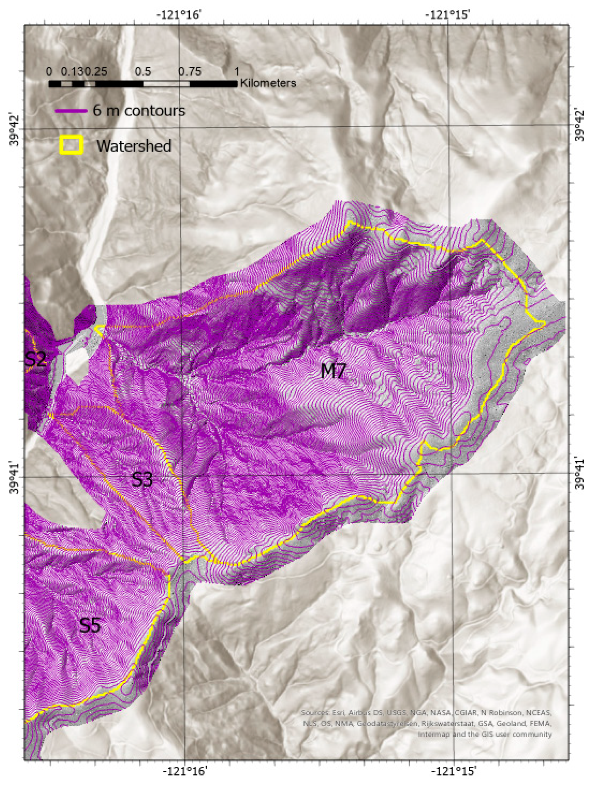
Sites analyzed in this study are located along the canyon section of the MF Feather River in Northern California. Accelerated uplift that occurred between 3.5–5 Ma caused the base-level lowering in the MF Feather River [32,33]. The study area has three distinct geomorphological domains as the landscape responds to the waves of aggression [34] that result from this base-level lowering. Landscape evolution along the MF Feather River plays a dominant role in debris flow formation and propagation throughout the drainage system impacted by the North Complex Fire (2020). The lower portion of the watersheds are topographically steeper and debris flows are more likely to reach the MF Feather River. Similarly, smaller sub-watersheds within these units are themselves generally steeper and debris flows can travel beyond their immediate watershed directly to the MF Feather River. The transitional domain occupies many of the tributary basins, thereby creating a steeper lower portion and a less steep upper portion of the watersheds as the energy line moves upstream in response to base-level lowering [35]. This has resulted in a landscape that currently exhibits a prominent convexity in the tributary watersheds. The upper watersheds have a lower-relief landscape with erosion rates an order of magnitude lower [36]. While slopes > 30° are found in the upper portion of the drainage, landslide propagation across lower slopes keep debris flows within the domain (Figure 2).
2.2. Watershed Selection
USGS watershed-scale probability of debris flow occurrence was used to randomly select the 8 medium and 5 small watersheds for this project [37]. Medium and small watersheds are based on a local measure of watershed area and would be considered small when compared with previous research from Japan [3]. The site selection was based on the drainage basin size and debris flow potential. The debris flow probability (greater than 0.83 for the chosen sites) was taken from the USGS debris flow assessment immediately following the 2020 North Complex Fire [37]. The USGS debris flow assessment used geospatial data related to basin morphometry, burn severity, soil properties, and rainfall characteristics to estimate debris flow probability in response to rainfall intensity, defined as rainfall with a peak 15-min rainfall intensity of 24 mm per hour (0.95 inches per hour) [38]. All watersheds in the USGS analyses are evaluated using the same rainfall intensity at the same time as a means of assessing the debris flow potential within each watershed.
2.3. Mapping of LWD
Lidar data were collected at a nominal density of 20 points per square meter (20 ppm2) and were referenced in NAD 1983 State Plane California I FIPS 0401 (US Feet) for the 13 watersheds. A 30 cm digital surface model (DSM) was generated from Class 1 data in the provider’s point cloud classification and 30 cm digital elevation model (DEM) generated from Class 2 in the provider’s point cloud classification. DSM and DEM data were produced using LAStools. The DEM was subtracted from the DSM in ArcGIS Pro v2.9.1. The subtracted raster surface can be classified based on elevation differences, whereby the LWD typically had an elevation difference signature ranging between 0.12 m to 1.3 m. Some variability in the elevation ranges occurred between watersheds because of the difference in species types, sizes, and degree of burning in each watershed. Classifying the elevation differences in this manner was done to remove a large portion of the data not identified as LWD on the ground without losing information to resolve the trees. The data extracted as LWD was classified as class 1 and all other data as class zero [39].
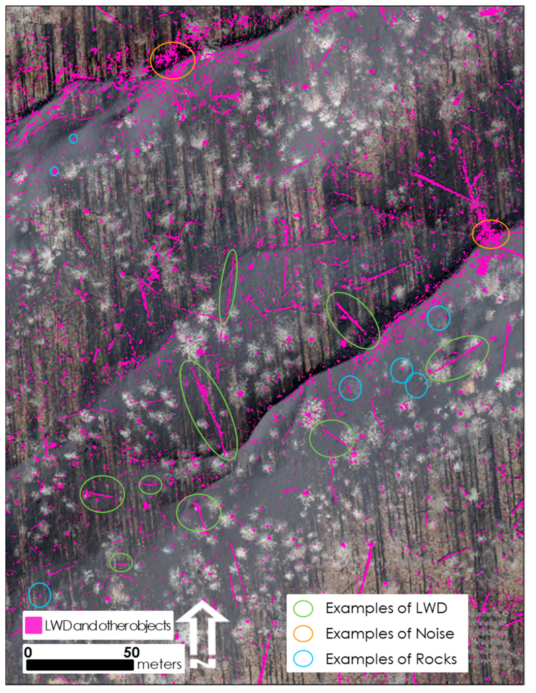
Not all non-LWD features in the subtracted surface could be removed. Rocks and rock outcrops represented a large portion of the isolated smaller objects in the results as well as areas that did not completely burn, which produced broader sections of noisy data, especially in steeper terrain (Figure 3). Noisy data were also identified along streams and in areas where riparian species did not completely burn or were partially burned (Figure 3). However, despite these identified shortcomings, trees are readily apparent in the classified data (Figure 3).
The final classified raster map containing LWD for each basin was overlayed on the debris flow pathway and used to determine where the LWD was intercepted and potentially transported by the debris flows along their pathways. Intercepted LWD was measured (length and width) to obtain information required by the LWD transport model used to examine the fate of LWD on the MF Feather River into Lake Oroville. In instances where there are questions concerning if the material was LWD or another feature, imagery gathered with the lidar data was used to aid in resolving the LWD and LWD measurements. This approach maximized our ability to capture LWD and reduce the potential for measuring other features along the debris flow pathways.
2.4. Debris Flow Modeling
DebrisFlow Predictor (DFP) is an agent-based simulation for shallow debris flows and debris avalanches [14] and developed by Stantec where the details of the model can be found [26]. It compares favorably to other models [40,41], and provides credible post-wildfire debris flow runout [29,30]. DFP predicts the flow path, the amount of scour and deposition along the entire path, and the inundation extent of debris flows. Landslide predictions are probabilistic and vary between runs, much as they do in nature. Multiple runs allow the user to, therefore, predict the scenario variability across the landscape.
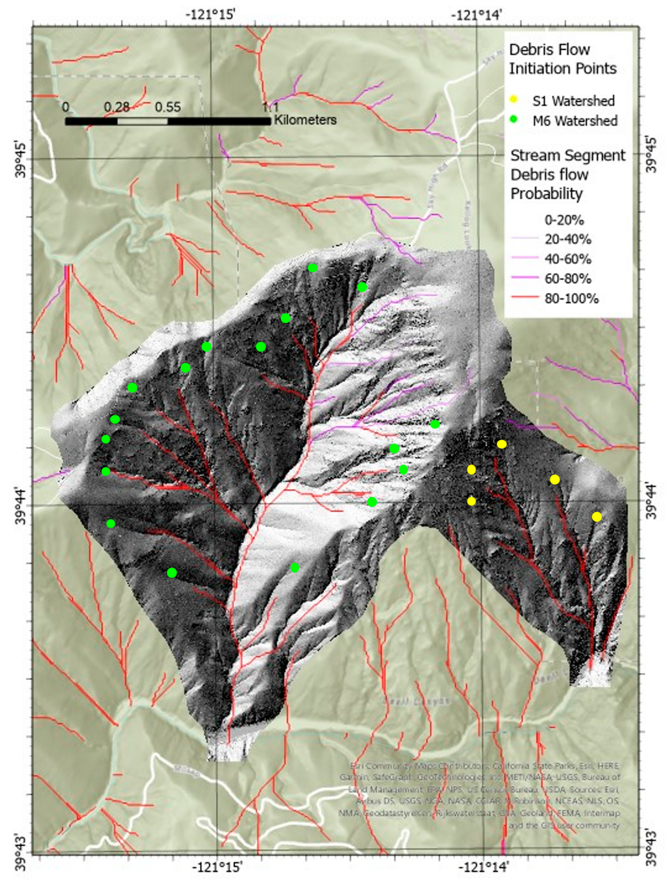
Debris flow likelihood along stream segments (produced in the USGS Debris Flow Hazard Assessment) within the 13 watersheds was used to establish debris flow initiation points for the model scenarios. Stream segments (greater than 0.4 km) with a greater than 80% probability of debris flows for rainfall intensities of 24 mm/h for 15 min [38] were selected to establish initiation points. A rainfall intensity of 24 mm/h for 15 min is approximately equivalent to the 50-year return event (NOAA Atlas 14) based on the watershed labeled M6 (Table 1).
Our model scenario established initiation points at locations upstream of all 80% probability stream segments where the initiation point was established in a location with a slope of >30° and high burn severity from the North Complex modified BARC data (Figure 4). The burn severity value is accepted within the research literature [42,43]. The slope value is slightly higher than that used by others in the scientific literature but is well within the range of slopes in which debris slopes initiate [14,44]. A higher slope value was selected to maximize debris-flow runout, given the disparity in slope within the medium watersheds and the steep nature of the small watersheds.
A five-meter resolution DEM was created and reformatted to an ASCII for use within DFP. Models were calibrated, run, and exported at this resolution. Debris flow runout lengths and deposits were initially calibrated to estimated depths and dimensions of recent fans (pre-fire and post-fire imagery) within the MF Feather River based on observations from Google Earth images and the recent imagery supplied along with the LiDAR data from California Department of Water Resources (CA DWR).
Initiation and sediment transport depths along the feeder channels in the watersheds were also calibrated from information gathered in these images. Initial model conditions were set-up based on past expert experience using DFP within this region, as well as testing the model with other known regional debris flows. Landslides were initiated by running the software (Go button) using continuous probabilities (Continuous Function) for debris scour and deposition. Fanning behavior, agent generation, erosion and deposition multipliers, momentum mass loss, and minimum initiation depths (agent settings) were determined in an iterative fashion until the results credibly matched the extent and depth of the historical debris flows and debris flow fans.
The final calibrated model settings in DFP contain standard debris flow fan parameters because the fan lengths and widths we assessed in the imagery and slopes measured from DEM data along the MF Feather River are comparable to previously observed debris flow fans we have modeled. Our sediment transport parameters represent a balance between 1—the thicker colluvial deposits (>0.5 m) on slopes in the upper watersheds and along some extents of the tributary streams, leading into the MF Feather River; and 2—the thinner layers of colluvium/alluvium (<0.5 m) or exposed bedrock found along sections of the feeder streams in both small and medium watersheds. Minimum initiation depths were selected because many of the streams were intermittent or ephemeral where little pore water pressure exists in the colluvium/alluvium found in the channels (increasing pore water in the sediment equates to a higher erosion likelihood) and because of the inconsistency of sediment availability along many streams, which would reduce the availability of thicker depths of sediment throughout the watershed.
DFP, as a software, does not identify or specifically incorporate LWD along the modeled debris flows. The debris flow was therefore assumed to incorporate LWD that it encountered along its path. Debris flow pathways, runout, and debris flow fan deposition were established for the scenario. The debris flow fan apex (the upper extent of the alluvial fan) was determined by where the feeder channel carrying the debris flow began to consistently widen proximal to the valley bottom of the MF Feather River.
Only LWD on the ground and readily available for transport were measured. No standing vegetation was measured because of the time required to measure both the standing tree dimensions and measuring the force required to erode and entrain the standing LWD. Subtracting the digital surface model (all LiDAR data points on the ground) from the digital elevation model (bare earth model—other ground objects filtered from the DSM) provided a means to select only LWD that would have been on the ground and available within the debris flow pathways. The LWD bridging the stream was removed in this process as it could have been outside the debris flow depths.
LWD from each debris flow pathway was measured for length and diameter in meters. The diameter was measured at approximately 0.5 m from the end on the widest section of the tree to attempt to provide some degree of consistency with measuring the burned trees on the ground. A combination of the DSM-DEM LWD layer and aerial imagery were used to establish the location of the LWD and make measurements in meters. All measured LWD was recorded in Excel files and converted to a.csv files for use in the LWD transport model.
Most of the trees within the debris flow pathway did not have root wads because many of the trees burned at the base. Root wad widths in non-burned environments are often measured because root wads inhibit LWD movement by anchoring the LWD to beds or banks and increasing frictional drag, thereby decreasing mobility [45]. Where root wads existed, the trees were often beyond the debris flow path and were not included in the volume estimations.
Only LWD with 1/3 of its length within the debris flow pathway were measured for transport. The literature on debris flow LWD recruitment was lacking conditions required to recruit LWD. Here, a decision was made that if 1/3 of the tree fell within the pathway of the debris flow, the LWD would be entrained and transported by the debris flow based on the expert judgment from other wildfires. Large flow volumes have been shown to entrain and transport large LWD for long distances [17,46]. While there is a large amount of LWD beyond debris flow pathways, studies have shown that much of the LWD associated with debris flows is derived from near the debris flow channel [47].
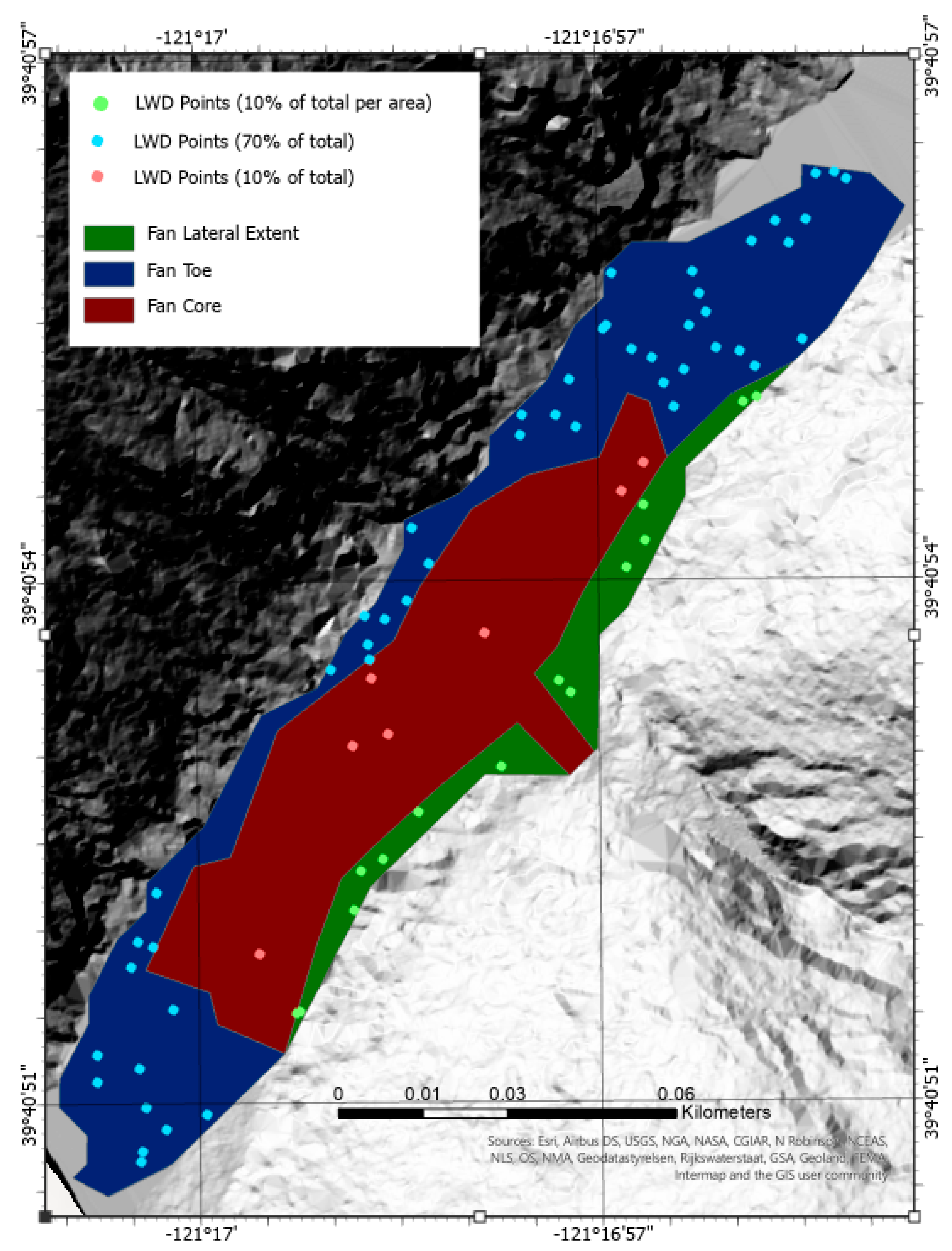
The LWD recorded along the debris flow pathways was randomly placed on the debris flow fan surface in a stratified manner. Debris flows often push LWD at the front of the debris flow surges. When exiting the feeder channel, some of the LWD will be pushed to the lateral extent of the fan (left and right), while the main mass of wood is transported to the distal portion (toe) of the debris flow fan [14,38].
The random placement of the wood in the fashion described above required mapping the fan as distinct areas. Debris flow fan perimeters were mapped for each fan. Four areas were identified within each fan perimeter (Figure 5). These areas consisted of two lateral extent areas (roughly where LWD would have been pushed to the lateral extent), the core of the fan (area with the highest probability of a debris flow occupying a raster cell), and the main flow areas in the toe of the debris flow fan (Figure 5). A total of 70% of the LWD from each watershed was randomly placed in the fan toe area and 30% of the total LWD was randomly placed in the two lateral extent areas (10% of the LWD in each) and core of the fan (10% of the LWD) (Figure 5). The decision for the proportionate distribution of the wood on the debris flow fan surface was based on an understanding of flow direction (from the modeling), where sediment mass was transported, and expert judgement from experience at other locations nationally and internationally. Randomly placing the points for the LWD locations in each of the areas was designed to capture the uncertainty in where the LWD would deposit within these fan areas and the ability to cluster the LWD within these locations. The Arcade create random points geoprocessing tool in ArcGIS Pro was used to generate the LWD points within the mapped areas. During the random point generation, the random points generator was permitted to establish zero space between points to simulate depositional clusters of LWD, which is also another common phenomenon evident in LWD transported by debris flows. Upon establishing the random points, x, y coordinates were added to all random points and exported as the coordinates for the LWD tables to be used in the LWD transport modeling.
2.5. LWD Transport Modeling
For the hydrodynamic simulation, a two-dimensional (2D) hydraulic model was developed using the HEC-RAS model, version 5.0.5 [48]. CA DWR supplied a 2D HEC-RAS model that includes the areas of interest for this analysis [49], hereafter referred to as the Frenchman Dam Model. The Frenchman Dam Model is a 2D HEC-RAS model to understand the flood extent downstream of the Frenchman Dam for two hypothetical failure scenarios: Frenchman Dam failure and Frenchman Spillway weir failure. This model includes the Frenchman Dam, which impounds Frenchman Lake, and the downstream floodplain to Lake Oroville.
The development of the 2D HEC-RAS model used some modeling parameters from the Frenchman Dam Model, with further refinement when necessary. A finer mesh resolution was required to properly resolve the channel geometry, and the detailed hydrodynamics within, rather than just the inundation extent compared with the original model. This analysis used a two-stage simulation approach to refine the lateral boundary of the river and achieves an optimal balance between model resolution and computational cost. The model was driven by the discharge at the river upstream, and a constant outflow of 289 cms was applied, which represents a sunny-day operation, as described in the Frenchman Dam Model.
The model domain extends upstream beyond the selected 13 watersheds within the MF Feather River where discharge data is available from the USGS gauge near Merrimac. Lake Oroville is included in its entirety, as the LWD are likely to be transported into the lake. The cross-sectional width of the river is very narrow in the upper reach of the MF Feather River, which requires a very high-resolution computational mesh on the order of 10 ft to adequately resolve the details required for the LWD hydrodynamic transport modeling.
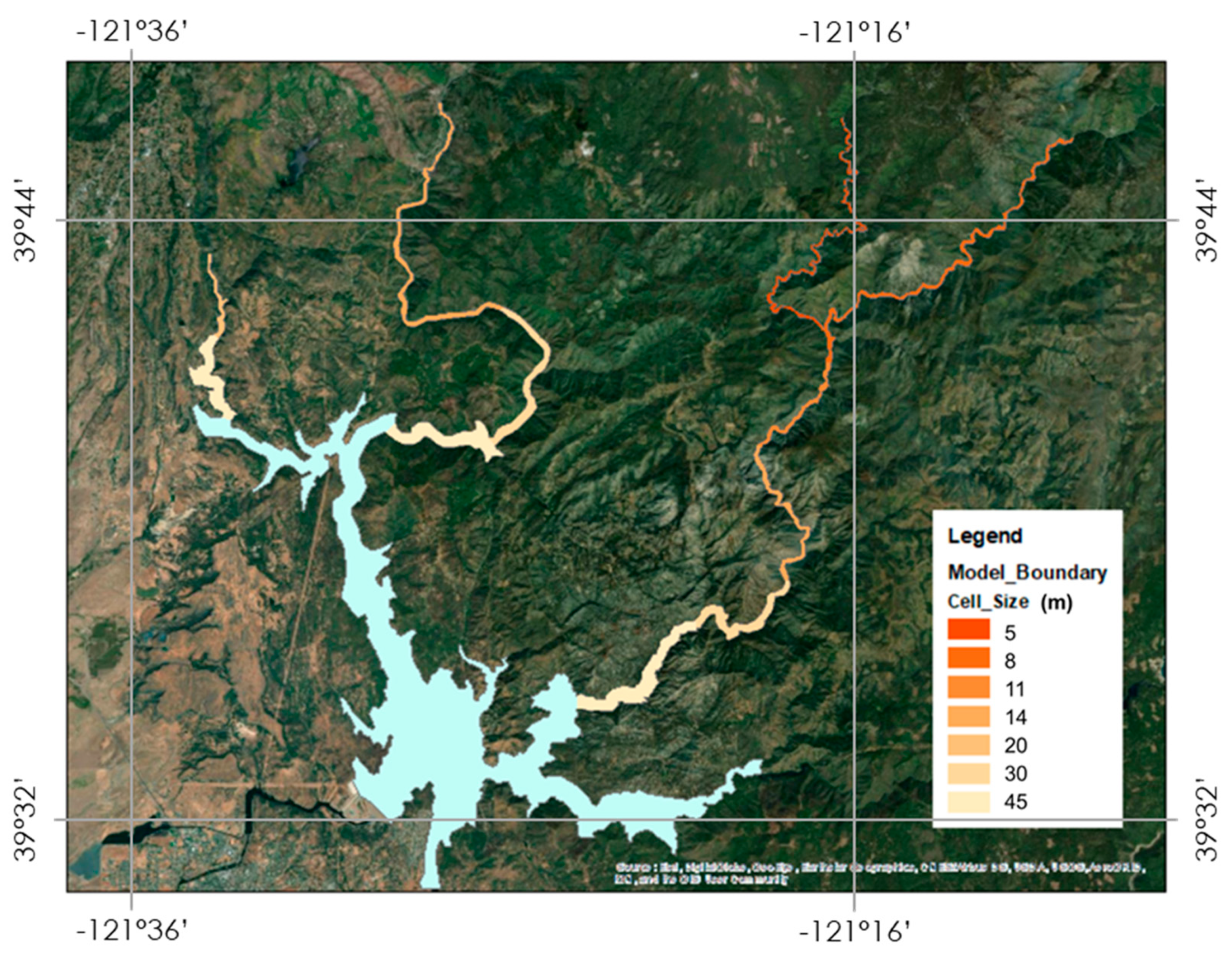
The initial lateral boundary and mesh resolution was based on the Frenchman Dam HEC-RAS model. The model was run at 1.5 times the 500-year event discharge, and the resulting maximum inundation boundary was used to update the lateral boundary. This refined the model boundary to the potential maximum flood extent, and the high-resolution computational cells can be allocated to resolve the narrow channel geometry. The overall mesh resolution for different sections of the model varies from 4.6 m at the most upstream reach of the MF Feather River to about 61 m for Lake Oroville (Figure 6). The model has a total of 102,000 computational cells.
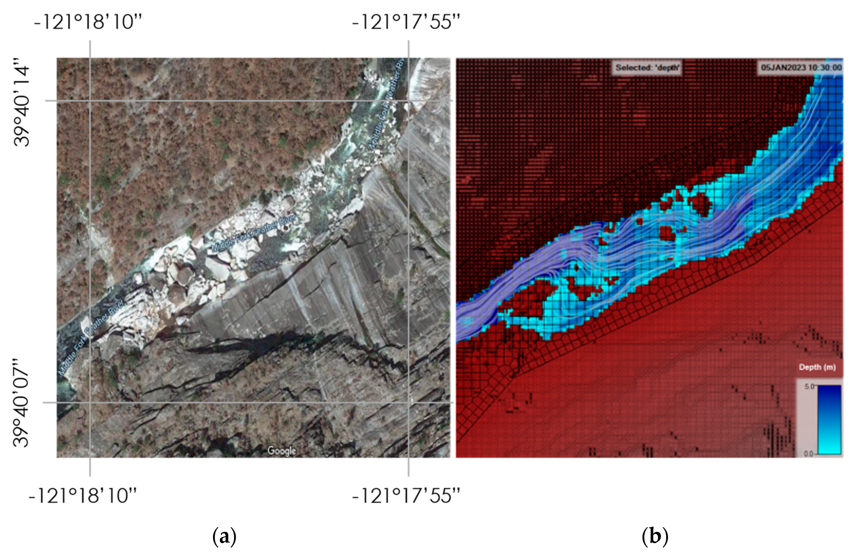
The hydrologic events with return periods of 1, 2, 5, 25, 50, 100, and 500 years were simulated with the refined 2D HEC-RAS hydrodynamic model. The corresponding discharge for the MF Feather River was obtained from the USGS stream gauge; while the discharge for other rivers were derived via a regression analysis using the available historical discharge records. The regression analysis showed a strong correlation of the discharge among the rivers within the domain of interest with the correlation coefficient for the peak discharge greater than 0.9. Details of the topographical features were resolved, and the corresponding flow patterns were captured by the model (Figure 7). Although there is no measured hydrodynamic data for model calibration, the modeling approach follows best practices, uses the best available information, and has a high mesh resolution.
Flow depths and velocity vectors from the 2D HEC-RAS model were used to transport the deposited LWD on the debris flow fan surface within the main trunk of the MF Feather River. The methods outlined for the use of the LWDSimR model were adopted here [23,50]. The LWDSimR model was converted into a Python code, which was coupled directly with the 2D HEC-RAS model, hereafter referred to as PyLWDSim. Like [23], the PyLWDSim and 2D HEC-RAS models were unilaterally coupled ignoring the feedback of LWD on the hydrodynamics. The simulation of LWD was calculated in two nested loops: 1—the function of the outer loop was to load the hydrodynamic results in terms of flow depths and velocity vectors at predefined output time steps from the 2D HEC-RAS model into the PyLWDSim model; and 2—the function of the inner loop was to calculate the transport processes of LWD at the much finer time steps required to resolve the transport processes. This procedure allowed LWD to be simulated with a higher temporal resolution than hydrodynamics. The hydrodynamic output was at 30-min intervals, while the time step for the transport process was determined dynamically such that each individual LWD does not travel more than one mesh cell of the hydrodynamic model grid to ensure model stability.
The recruitment, entrainment, and transport of LWD was hydrodynamically driven. The flow depth and velocity vector were needed at the location of each piece of LWD for a given time, since the hydrodynamics were computed and saved at fixed grid locations from the 2D HEC-RAS model. This was achieved through a bilinear interpolation using the hydrodynamic output at the nearest three mesh nodes that triangulate each LWD. The flow depth and velocity vector at the location of each LWD were then used to determine the hydrodynamic recruitment, entrainment, and transport process of the LWD.
The recruited or downed trees may be entrained in the water column because of flow. This was determined based on the balance of hydrodynamic (F) and resistance forces (R) on individual LWD pieces according to [51]. With the assumption that each LWD piece was positioned perpendicular to the flow direction, the hydrodynamic force F can be written as
where is the drag coefficient for the LWD in water, is the density of water, is the diameter of the LWD, h is the flow depth, U represents velocity magnitude, and the length of the LWD is expressed as . The density of the wood element is assumed to be close to that of water. The resistance forces can be estimated as
where g is gravitational acceleration, is the friction coefficient between the LWD and the channel bed, and the submerged area of the log perpendicular to its length can be defined as
The balance between the hydrodynamic force and resistance force can then be expressed using a non-dimensional factor as
The condition that yields the balance of the hydrodynamic and resistance force, i.e., , is the critical condition, and the threshold velocity for the movement of the LWD is then expressed as
The following simplified scheme was considered according to [52]:
Case I: If , the LWD piece is floating, with the associated transport inhibition parameter c = 0.
Case II: If , and , the LWD piece is resting, with the associated transport inhibition parameter c = 1.
Case III: If , and , the LWD piece is either rolling or sliding, with the associated transport inhibition parameter expressed as
and the velocity along the transport trajectory for each moving LWD piece is estimated as follows:
The transport velocity can then be used to calculate the new position for every transported LWD at each time step. A moving LWD piece can be deposited at a particular time step if the conditions for entrainment were no longer fulfilled, and the LWD can be remobilized in a subsequent time step.
The model parameters were specified in the text input file, which includes the project description path to the 2D HEC-RAS output HDF file; the hydrodynamic basin name defined in the 2D HEC-RAS model; the output time interval for hydrodynamics results; the starting time for LWD transport modeling in terms of the number of hydrodynamic output time intervals, such that the hydrodynamic model is stable; the LWD transport modeling duration in terms of number of hydrodynamic output time intervals; the path to LWD input; and the path to the output folder. The LWD input was a CSV file containing the following information for each recruited LWD piece from the debris flow predictor model:
- ID: Unique identifier for each LWD as a sequential integer.
- Watershed: The name of the watershed where the LWD originates.
- Xcoord and Ycoord: The initial x- and y-coordinate of the LWD in the debris flow fan areas.
- DBH: The diameter of the LWD piece at breast height.
- Status: Status of the tree, which is classified as 1 = rooted, 2 = lying, 3 = moving, 4 = jammed. The initial status of living wood is always 1 and that of dead wood is 2.
- Rootwad: The diameter of Rootwad of the LWD piece.
- Length: The length of the LWD piece.
- Structure: The wood structure for a standing tree.
- Slope: The geomorphologic characteristics of the areas for the LWD of piece.
The model output contained the location, status, characteristics, and hydrodynamics of all LWD pieces at every five timesteps to allow for a detailed understanding of the temporal transport dynamics. The output data were used in post-processing to determine the transport path and fate of the LWD at any time during the simulation.
The fate of the LWD was also analyzed to understand the volume of LWD and the corresponding transport ratio of the LWD, defined as the mobilized or relocated volume of LWD at any given time (or the volume of LWD that reach Lake Oroville at the end of simulation as a special case) to the total available LWD from the debris flow model. The relatively narrow river cross-section width of the MF Feather River, which was comparable to the length of some large LWD, especially within the upper reaches of the MF Feather River required an adjustment to be made to the transport ratio from the model output. The adjustment to the transport ratio addresses a model limitation whereby the dimension of the LWD was not accounted for throughout the LWD transport along the MF Feather River and ultimately provided a more realistic simulation of the LWD fate. For each LWD transported along the MF Feather River, the length of the LWD was compared with the most critical cross-section (narrowest width) downstream from its origin. Should the length of the LWD be greater than the critical width, the LWD was removed from the account. The transport ratio was then recalculated with the remaining LWD to mimic sorting of LWD along the flow pathway towards Lake Oroville.
For each hydrologic event, the transport ratio of LWD was defined as the volume of LWD that reached Lake Oroville from a watershed to the total initial volume of LWD within that watershed, as well as the total transport ratio accounting for all LWD in all watersheds. The transport ratios were calculated directly using the model output, which was identified as ‘no adjustment’. They were also calculated by removing the pieces with a length greater than the critical cross-section width of the river, following the approach discussed in the Sub-Scenario of the LWD Transport Modeling, which was identified as ‘adjusted’.
3. Results
3.1. LWD Transport via Debris Flows
A total of 1073 pieces of LWD potentially would be transported via debris flows from the 13 modeled watersheds to the MF of the Feather River. The small watershed had lesser debris flow volumes (Table 2). Medium watersheds produced a total of 889 pieces of LWD compared with 116 pieces of LWD from the small watersheds. Medium watersheds produce 111 pieces of LWD on average (range was 13 to 194 pieces of LWD), while the small watersheds produced 37 pieces of LWD on average (range was 7 to 81 pieces of LWD). Small watersheds produced more LWD than some of the medium watersheds despite possessing ½ the drainage area of most of the medium watersheds. There was a weak positive trend between the debris flow volume and the LWD volume (Table 2). All LWD volumes were below 1% of the debris flow volumes except for watershed M3, which was an outlier making up 5% of the total volume.
3.2. LWD Transport and Fate along the MF of Feather River and into Lake Oroville
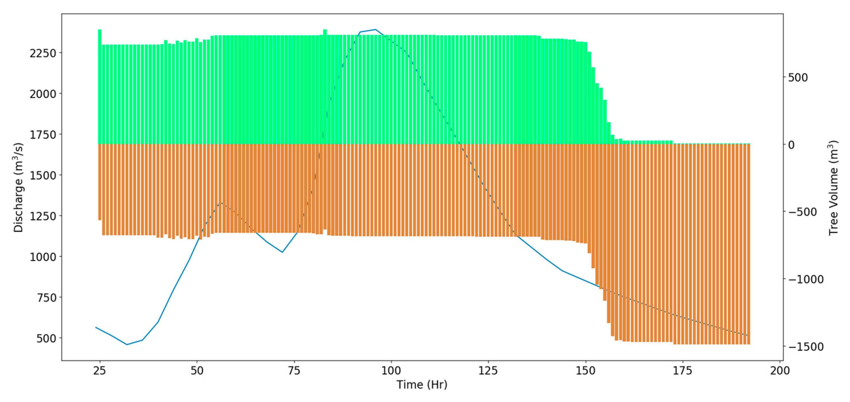
The temporal LWD transport dynamics were illustrated as the volume of LWD that mobilized versus the volume of LWD that deposited for a given time during the simulation (Figure 8). A significant amount of LWD was mobilized within the first few time steps of the simulation and some deposition was observed along the banks of the river. As the discharge increased, new and/or previously deposited LWD were mobilized. During the falling limb of the hydrograph, especially at the tail end, mobilized LWD were transported downstream and eventually deposited after reaching the lower boundary of the model at the dam.
The spatial distribution of LWD was first analyzed using a raster that shows the volume of LWD passing through a fixed raster cell at a resolution of 3 m, referred to as the transport path volume raster. Figure 9 shows the flow path volume raster for the 50-year event. The transport path was concentrated along the main channel of the river, especially for the upper reach of the MF Feather River, but spread after reaching the wider section at the lower reach adjacent to Lake Oroville. The transport path eventually ended along the dam with LWD deposited near the entrance of spillway. The effects of wind and the corresponding surface flow that may further spread the LWD within Lake Oroville were not considered in the LWD transport modeling.
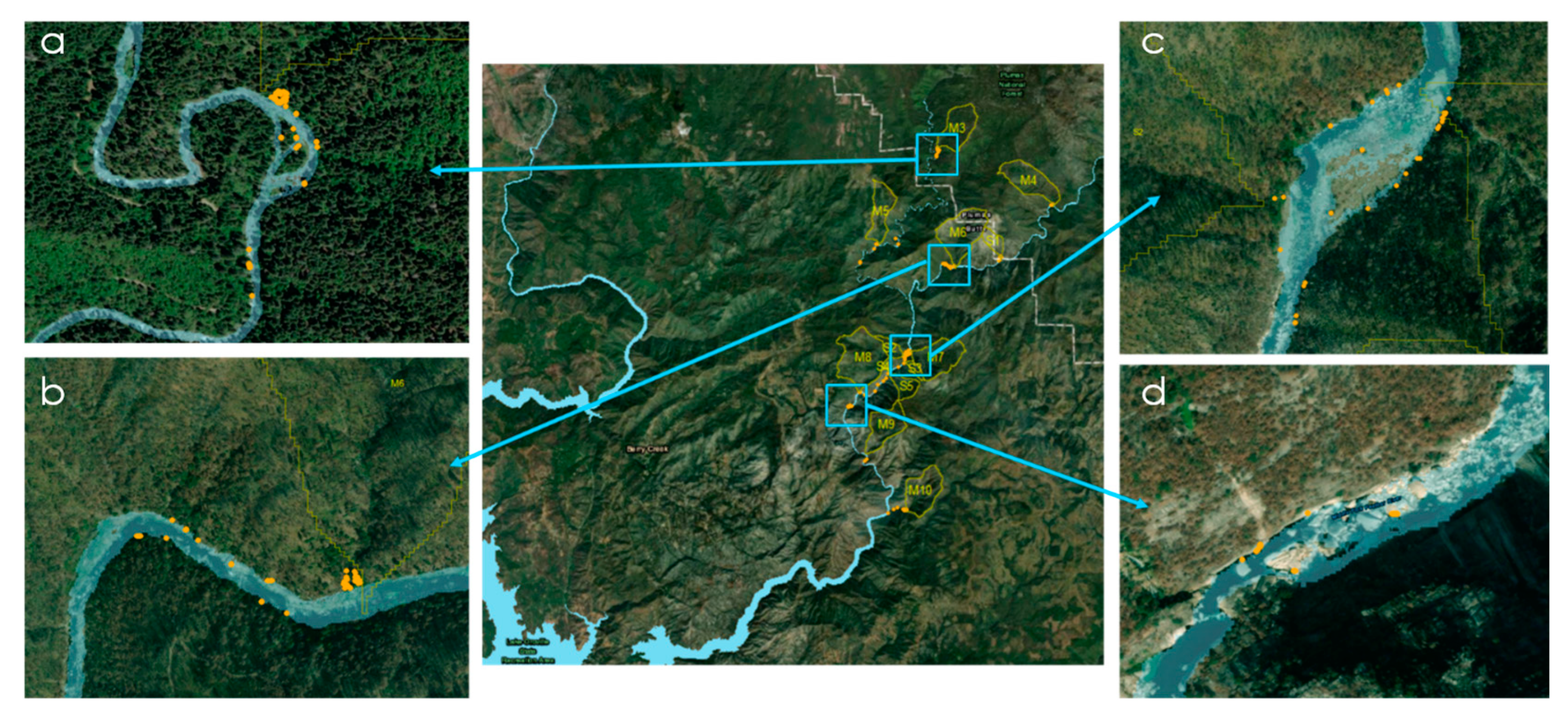
Most of the LWD ends up in Lake Oroville (Figure 9, Figure 10, Figure 11 and Figure 12), some LWD were trapped within the MF Feather River (Figure 10). LWD also remained at their initial location as the flow did not reach the full extent of the debris flow fan surface, especially for watersheds M3, M5, and M10, which are located at small branches of the MF Feather River with much smaller discharges. LWD was deposited near the banks approaching river bends or after cross-section expansion (Figure 10). LWD was also trapped at locations with large bed rocks (Figure 10).
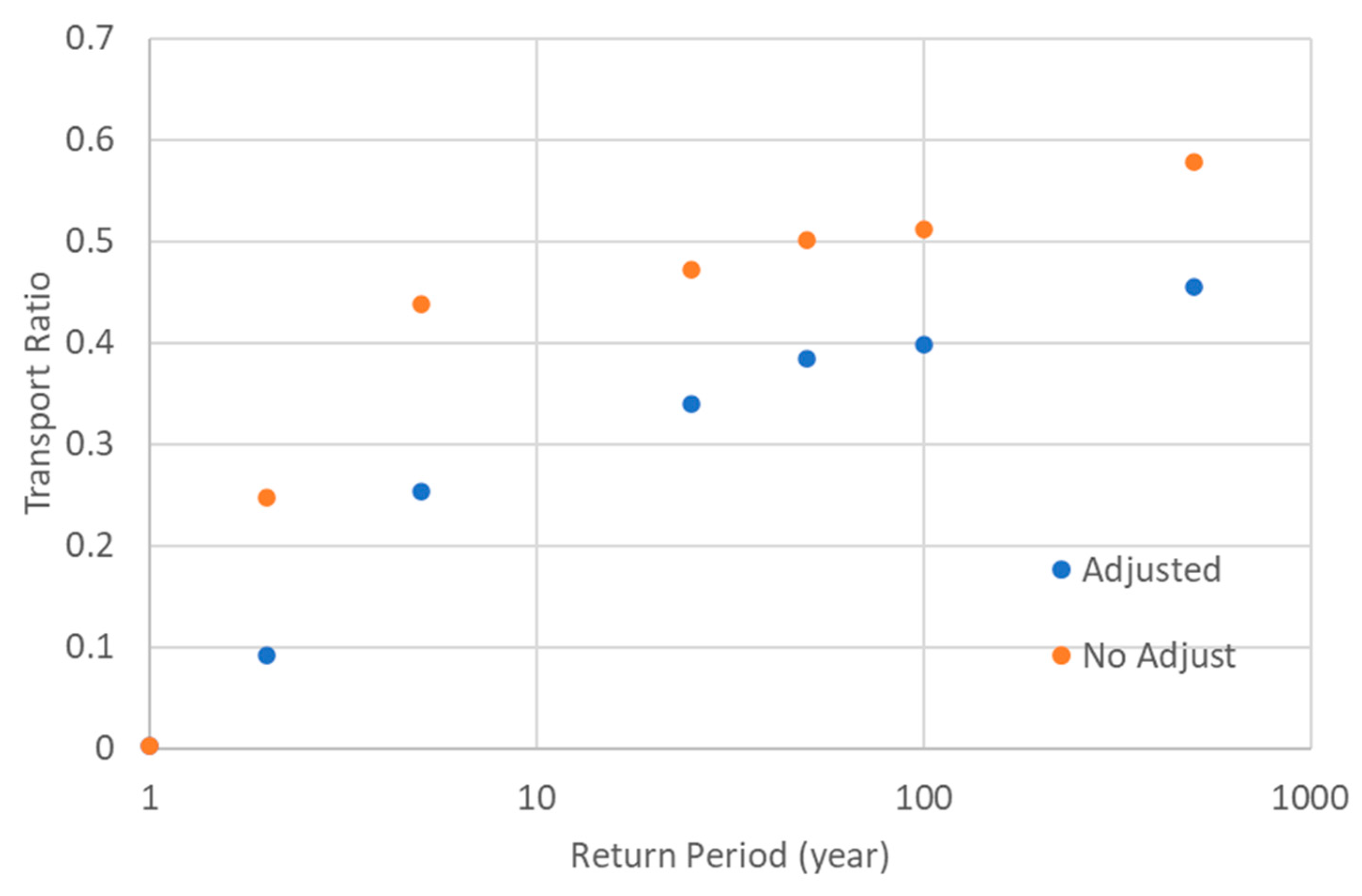
The transport ratio of LWD increased with an increasing return period, which was expected as higher discharge causes greater depth, flow velocities, and transporting power (Table 3). Few LWD were transported into Lake Oroville during the 1-year event. LWDs started to be transported to Lake Oroville during the 2-year event, where the total transport ratio was estimated to be 9% to 25%, with and without adjustment (Table 3). The transport ratio increased to 46% to 58% for the 500-year event (Figure 11 and Figure 12).
3.3. Comparison to Previous LWD Removals from Lake Oroville
Historically, LWDs within Lake Oroville had been removed on an annual basis during most years when regular storms occurred. The intensity of the storms was not documented, but the removed LWD were placed on a pile with an area of 10 hectares and a height typically reaching 1.21 m for most years and less for others. The debris was not collected in 2022 due to the lack of storms, as communicated by CA DWR. The packing ratio of the wood pile, defined as the ratio of wood volume to the total pile volume, ranges from 0.06 to 0.26, which can be higher for clean piles with larger logs [53]. Assuming a packing ratio of 0.25, the removed LWD volume was estimated as
The selected 13 watersheds with past wildfires had a total drainage area of 21 sq km, while the total burned area for the North Complex Fire was 1191 sq km. Using the estimated total volume of LWD from the 13 watersheds and the transport ratio from the PyLWDSim model, the total volume of LWDs from all burned watersheds that enter Lake Oroville can be estimated with a simple extrapolation based on the ratio of the drainage area (Table 4). Since the previous removals occurred for most years but not all, it is reasonable to compare that to high frequency events such as a 2-to-5-year event, where the estimated total transported volume of LWDs in Lake Oroville ranges from 274 m3 to 42,141 m3 with adjustment and 274 m3 to 53, 467 m3 without, which was consistent with the estimated historical removal volume.
4. Discussion
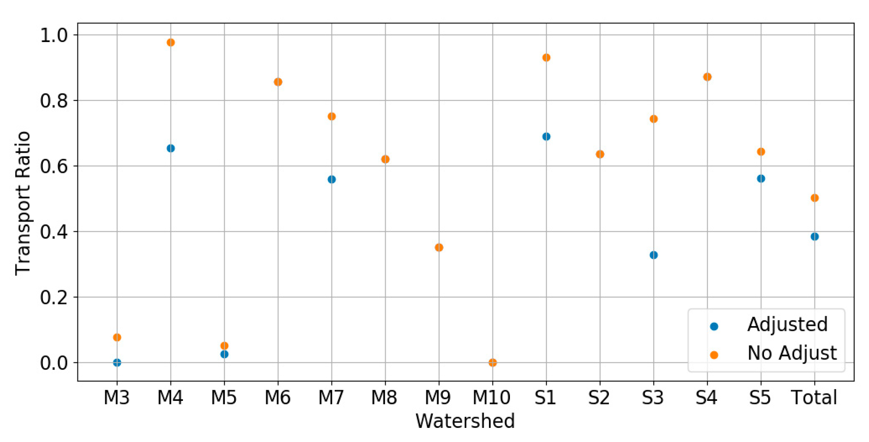
The LWD transport modeling showed the potential for a major portion of the LWD available arriving in Lake Oroville for both the LWD jam and non-jam scenarios. Consistent with previous research [4], our model results showed the largest volume of LWD transported to Lake Oroville was associated with the largest flood. In our LWD jam modeling scenario the 5-year event transports 25% of the LWD brought to the MF Feather River via debris flows to the reservoir. The 25-year, 50-year, and 100-year flood events fall within the range of 34% to 39% (increasing with flood magnitude) indicating that floods with these return intervals have the potential to transport significant amounts of LWD to Lake Oroville. Some watersheds did not have strong connectivity with the MF Feather River or did not have significant volumes of LWD transported to the debris flow fans. The watersheds with higher connectivity often exhibit transport ratios greater than 60%, with several watersheds (five in total) with transport ratios greater than 80%. The differences in connectivity are likely representative of what is happening within the system and reflect our current understanding of connectivity [53].
The above numbers also highlight that not all LWD was transported to the reservoir. Some of the tributaries that did not have high connectivity with the MF of the Feather River were small systems that did not produce discharges to transport the LWD to the mainstem river. Entrained LWD not arriving at the reservoir was often deposited and stored on mid-channel bars, trapped by large boulders in the channel, deposited at the beginning of an outer bend of a meander, or deposited in reaches where the channel width expanded. These findings support previous work that shows LWD jams in similar locations within another region of California [5]. In other instances, LWD was also not entrained from the debris flow fan surfaces, as the flood elevation was not high enough to entrain the LWD located outside of the flood extent. As no bridges were present along the mainstem river, these structures did not play a significant role in trapping LWD being transported along the MF Feather River, as has been identified in previous studies [17].
The debris flow modeling, while critical to the understanding the LWD transport from tributaries to the mainstem streams, also highlights the importance of sediment transport from this process. Sediment transport was not a component of this study along the MF Feather River. However, inferences can be made given our observations and previous experience. Analysis of the canyon section of the MF Feather River shows limited sediment storage. Major portions of the debris flow fan deposits would be transported along with the LWD during flooding. This has implications for the MF Feather River, as large particles transported by the debris flows will likely be left behind in the vicinity of the debris flow fan to form rapids. Should rocks within these areas protrude through or be close to the water surface, these might serve as potential locations for trapping LWD from upstream. Sediment transported from the debris flow fans can change downstream channel morphology through the development of new bars or the expansion of existing bars (lateral, mid-channel, and point bars). There is also the potential for transporting large amounts of sediment from the debris flow fans to the reservoir during a flood, as on average the modeled debris flow fans had 695,830 m3 of material stored in them.
The models were based on some simplifications and assumptions. We attempted to reduce the epistemic uncertainty from not knowing or not having information available to resolve all the potential dynamics within the systems. In the debris flow modeling multiple predictive simulations and probabilistic approaches were used to reduce uncertainty and enhance our ability to represent the system dynamics. The debris flow model represents our best effort to identify the locations and magnitudes of credible scenarios for debris flow initiation, runout, and inundation. Despite the diligence, the following are limitations to our modeling approach for the debris flow transport of LWD:
- Debris flow fan development was impacted by the lack of LiDAR data in the channel of the MF Feather River. The faceted DEM at this location had an impact of debris flow formation and these represent a best approximation of the surficial feature at these locations.
- There were heavily burned standing trees along the channels that were not incorporated into the counts of LWD. These could become a potential source of LWD as they fall into channels through the undercutting of the stream bank, wind throw, or as the trees decompose over time. These will continue to provide a supply of LWD to the system over time.
- There were locations along the watershed valley bottoms where LWD sampling was inhibited by “noisy” LiDAR data associated with dense lower canopy vegetation and in some instances these areas were in shadows within the imagery because of the time of day the aerial photographs were taken. In both instances, the LWD population through these areas was likely underrepresented.
- We assumed entrained LWD in our modeling approach made it out of the medium and small watersheds to the MF Feather River. This was a limitation in the approach, as we were unable to account for terrain conditions where the LWD might have been trapped behind large rocks or jammed behind trees and between the banks. This could lead to an overestimation of the amount of LWD from the ground that would be transported to the MF Feather River. However, even with this limitation, we were likely underestimating the total magnitude of LWD because the burned standing trees are not accounted for in this measurement.
Similarly, there are limitations to the LWD transport modeling. The transport dynamics and fate of the LWD within the Lake Oroville watersheds were studied using the PyLWDSim model based on previous methods [50] where the hydrodynamics were derived using the 2D HEC-RAS model. There are some limitations intrinsic to the data availability, model assumption, and simplification that may affect the accuracy of the analysis.
- The hydrodynamics were derived using the 2D HEC-RAS model, where the following limitations for the application to the hydrodynamic transport of LWD were identified:
- The hydrodynamic was resolved at the resolution of the bathymetry data.
- The hydrodynamic model lacked validation due to limited data although the best practices were followed for model setup, parameterization, etc.
- The influence of wind on the surface velocity was not included in the hydrodynamic model where the resulting surface flow can change the path of the LWD within Lake Oroville.
- The hydrodynamic was unilaterally coupled with the transport model such that the influence of the LWD on the hydrodynamics is not accounted for. This may have resulted in poor results where the river channels were jammed by LWD.
- The hydrodynamic transport of LWD was a very complex process involving LWD recruitment due to the hydro-dynamic, entrainment, transport, and deposition of LWD, and obstruction of LWD.
- The initial LWD position was randomly distributed within the main trunk of the river, which requires further investigation via field survey.
- The hydrodynamic recruitment process was based on a probabilistic approach rather than a physical based solution, although this does not apply to this study, as all LWD applied in this analysis were recruited from the hillside due to a landslide.
- The length or dimension of the tree is not directly modeled, which means:
- a.
- Interactions between trees, with large rocks on the stream bed, and logs breaking were not accounted for in this model.
- b.
- Limitations are at the narrow section of the river when the river width was on the same order of LWD length or less. Attempts have been made to account for this empirically by adjusting the estimated transport rate, removing the LWD that have the lengths longer than the restricted cross section width downstream from their origin.
- c.
- Underestimation may also be caused by neglecting other processes such as sediment transport and morphology changes during the flood event.
5. Conclusions
The meshing together of multiple process-based models provided a means to understand the potential transport pathways and fate of LWD following a wildfire to Lake Oroville, a reservoir impounded by the largest earth-fill dam in the United States. LWD was transported via debris flows from tributary streams to the MF Feather River and deposited on debris flow fans. Flood hydrodynamics in conjunction with LWD entrainment and transport modeling provided an understanding of the potential pathways and volumes of material moving along the MF Feather River and into Lake Oroville. There is the potential for 25% to 46% of the total amount of LWD deposited on the debris flow fans reaching Lake Oroville in our scenario that tried to account for LWD jams in the simulated 5-year and 500-year flood events. The narrow channel along the MF of the Feather River helps maintain deeper flow depths and higher velocities throughout the extent of the river course examined and this led to the high transport ratios identified in the reservoir. Not all LWD made it to the reservoir and the study identified key locations where LWD is stored along the transport pathways.
Author Contributions
Conceptualization, T.W., A.C. and R.H.G.; methodology, T.W., A.C. and R.H.G.; software, R.H.G. and A.C.; validation, T.W. and A.C.; formal analysis, T.W. and A.C.; writing—original draft preparation, T.W., A.C. and R.H.G.; writing—review and editing, T.W., R.H.G. and A.C.; visualization, T.W. and A.C.; supervision, T.W., A.C. and R.H.G.; project administration, T.W. and A.C.; funding acquisition, T.W., A.C. and R.H.G. All authors have read and agreed to the published version of the manuscript.
Funding
This research was funded by the California Department of Water Resources under TO#23 Woody Debris Modeling for Lake Oroville.
Data Availability Statement
Lidar data, aerial images, and HEC model were supplied by California Department of Water Resources. The LWDsimR can be found as open access software at https://zenodo.org/record/1296733 (accessed on 3 Novermber 2021).
Acknowledgments
The authors are grateful to the California Department of Water Resources providing us the opportunity to explore our methods and science throughout this project. We also wanted to recognize the project managers from the California Department of Water Resources and Stantec (Matt Powell) as well as other support staff from Stantec for making this project happen and making sure it was completed on time.
Conflicts of Interest
The authors declare no conflict of interest. The project funder contracted the lidar and aerial imagery data. The contracted company performed all the data collection and processing. The project funder provided the HEC model used in this project. The methods and analyses were all designed and carried out by the authors. Updates of our progress with this research were presented to the project funder.
References
- Zelt, R.B.; Wohl, E.E. Channel and woody debris characteristics in adjacent burned and unburned watersheds a decade after wildfire, Park County, Wyoming. Geomorphology 2004, 57, 217–233. [Google Scholar] [CrossRef]
- Short, L.E.; Gabet, E.J.; Hoffman, D.F. The role of large woody debris in modulating the dispersal of a post-fire sediment pulse. Geomorphology 2015, 246, 351–358. [Google Scholar] [CrossRef]
- Seo, J.I.; Nakamura, F.; Nakano, D.; Ichiyanagi, H.; Chun, K.W. Factors controlling the fluvial export of large woody debris, and its contribution to organic carbon budgets at watershed scales. Water Resour. Res. 2008, 44, W04428. [Google Scholar]
- Ruiz-Villanueva, V.; Gibaja, J.; Piégay, H. Instream large wood at the Génissiat dam reservoir: From problems to opportunities. In Proceedings of the 39th IAHR World Congress, Granada, Spain, 19–24 June 2022; pp. 2730–2734. [Google Scholar] [CrossRef]
- Iskin, E.P.; Wohl, E. Wildfire and the patterns of floodplain large wood on the Merced River, Yosemite National Park, CA, USA. Geomorphology 2021, 389, 107805. [Google Scholar] [CrossRef]
- Berg, N.; Azuma, D.; Carlson, A. Effects ofwildfire on in-channelwoody debris in the Eastern Sierra Nevada, California. In Proceedings of the Symposium on the Ecologyand Management of Dead Wood in Western Forests, Reno, NV, USA, 2–4 November 1999; USDA Forest Service: Asheville, NC, USA, 1999. [Google Scholar]
- Wohl, E.; Marshall, A.E.; Scamardo, J.; White, D.; Morrison, R.R. Biogeomorphic influences on river corridor resilience to wildfire disturbances in a mountain stream of the Southern Rockies, USA. Sci. Total Environ. 2022, 820, 153321. [Google Scholar] [CrossRef]
- Chen, X.; Wei, X.; Scherer, R. Influence of wildfire and harvest on biomass, carbon pool, and decomposition of large woody debris in forested streams of southern interior British Columbia. For. Ecol. Manag. 2005, 208, 101–114. [Google Scholar] [CrossRef]
- Marcus, W.A.; Rasmussen, J.; Fonstad, M.A. Response of the Fluvial Wood System to Fire and Floods in Northern Yellowstone. Ann. Assoc. Am. Geogr. 2011, 101, 21–44. [Google Scholar] [CrossRef]
- Shakesby, R.; Doerr, S. Wildfire as a hydrological and geomorphological agent. Earth-Sci. Rev. 2006, 74, 269–307. [Google Scholar] [CrossRef]
- Kean, J.W.; Staley, D.M. Forecasting the Frequency and Magnitude of Postfire Debris Flows Across Southern California. Earth’s Futur. 2021, 9, e2020EF001735. [Google Scholar] [CrossRef]
- Booth, A.M.; Sifford, C.; Vascik, B.; Siebert, C.; Buma, B. Large wood inhibits debris flow runout in forested southeast Alaska. Earth Surf. Process. Landf. 2020, 45, 1555–1568. [Google Scholar] [CrossRef]
- Yamazaki, Y.; Egashira, S. Run Out Processes of Sediment and Woody Debris Resulting from Landslides and Debris Flow. In Proceedings of the 7th International Conference on Debris-Flow Hazards Mitigation, Golden, CO, USA, 10–13 June 2019; Special Publication 28. Association of Environmental and Engineering Geologists: Sacramento, CA, USA, 2019. [Google Scholar]
- Rusyda, M.I.; Ikematsu, S.; Hashimoto, H. Woody debris production and deopsition during flood at extreme rainfall period 2012-2013 in Yabe and Tsuwano River Basin, Japan. Indones. J. Geogr. 2020, 52, 290–305. [Google Scholar] [CrossRef]
- Benda, L.; Bigelow, P. On the patterns and processes of wood in northern California streams. Geomorphology 2014, 209, 79–97. [Google Scholar] [CrossRef]
- Wester, T.; Wasklewicz, T.; Staley, D. Functional and structural connectivity within a recently burned drainage basin. Geomorphology 2014, 206, 362–373. [Google Scholar] [CrossRef]
- Comiti, F.; Lucía, A.; Rickenmann, D. Large wood recruitment and transport during large floods: A review. Geomorphology 2016, 269, 23–39. [Google Scholar] [CrossRef]
- Kang, T.; Kimura, I.; Onda, S. Application of computational modeling for large wood dynamics with collisions on moveable channel beds. Adv. Water Resour. 2021, 152, 103912. [Google Scholar] [CrossRef]
- Ruiz-Villanueva, V.; Wyżga, B.; Zawiejska, J.; Hajdukiewicz, M.; Stoffel, M. Factors controlling large-wood transport in a mountain river. Geomorphology 2016, 272, 21–31. [Google Scholar] [CrossRef]
- Ruiz-Villanueva, V.; Gamberini, C.; Bladé, E.; Stoffel, M.; Bertoldi, W. Numerical modeling of instream wood transport, deposition, and accumulation in braided morphologies under unsteady conditions: Sensitivity and high-resolution quantitative model validation. Water Resour. Res. 2020, 56, e2019WR026221. [Google Scholar] [CrossRef]
- Kang, T.; Kimura, I.; Shimizu, Y. Numerical simulation of large wood deposition patterns and responses of bed morphology in a braided river using large wood dynamics model. Earth Surf. Process. Landf. 2020, 45, 962–977. [Google Scholar] [CrossRef]
- Persi, E.; Petaccia, G.; Fenocchi, A.; Manenti, S.; Ghilardi, P.; Sibilla, S. Hydrodynamic coefficients of yawed cylinders in open-channel flow. Flow Meas. Instrum. 2019, 65, 288–296. [Google Scholar] [CrossRef]
- Zischg, A.P.; Galatioto, N.; Deplazes, S.; Weingartner, R.; Mazzorana, B. Modelling spatiotemporal dynamics of large wood recruitment, transport, and deposition at the river reach scale during extreme floods. Water 2018, 10, 1134. [Google Scholar] [CrossRef]
- Rickenmann, D.; Laigle, D.M.B.W.; McArdell, B.W.; Hübl, J. Comparison of 2D debris-flow simulation models with field events. Comput. Geosci. 2006, 10, 241–264. [Google Scholar] [CrossRef] [Green Version]
- McDougall, S. Canadian Geotechnical Colloquium: Landslide runout analysis—Current practice and challenges. Can. Geotech. J. 2017, 54, 605–620. [Google Scholar] [CrossRef] [Green Version]
- Guthrie, R.; Befus, A. DebrisFlow Predictor: An agent-based runout program for shallow landslides. Nat. Hazards Earth Syst. Sci. 2021, 21, 1029–1049. [Google Scholar] [CrossRef]
- Barnhart, K.R.; Jones, R.P.; George, D.L.; McArdell, B.W.; Rengers, F.K.; Staley, D.M.; Kean, J.W. Muti-Model Comparison of Computed Debris Flow Runout for the 9 January 2018 Montecito, California Post-Wildfire Event. J. Geophys. Res. Earth Surf. 2021, 126, e2021JF006245. [Google Scholar] [CrossRef]
- Floyd, I.E.; Sanchez, A.; Gibson, S.; Savant, G. A modular, non-Newtonian, model, library framework (DebrisLib) for post-wildfire flood risk management. Hydrol. Earth Syst. Sci. Discuss. 2020, 1–21. [Google Scholar]
- Wasklewicz, T.; Guthrie, R.H.; Eickenberg, P.; Kramka, B. Lessons learned from the local calibration of a debris flow model and importance to a geohazard assessment. In Proceedings of the Geohazards 8 Conference Proceedings, Quebec City, QC, Canada, 12 June 2022; pp. 333–337. [Google Scholar]
- Wasklewicz, T.; Guthrie, R.H.; Eickenberg, P.; Kramka, B. Modeling Post-wildfire Debris Flow Erosion for Hazard. Environ. Connect. 2022, 22–24. [Google Scholar]
- Murphy, B.P.; Czuba, J.; Belmont, P. Post-wildfire sediment cascades: A modeling framework linking debris flow generation and network-scale sediment routing. Earth Surf. Process. Landf. 2019, 44, 2126–2140. [Google Scholar] [CrossRef]
- Wakabayashi, J.; Sawyer, T.L. Stream Incision, Tectonics, Uplift, and Evolution of Topography of the Sierra Nevada, California. J. Geol. 2001, 109, 539–562. [Google Scholar] [CrossRef] [Green Version]
- Stock, G.M.; Anderson, R.S.; Finkel, R.C. Pace of landscape evolution in the Sierra Nevada, California, revealed by cosmogenic dating of cave sediments. Geology 2004, 32, 193–196. [Google Scholar] [CrossRef] [Green Version]
- Brunsden, D. A critical assessment of the sensitivity concept in geomorphology. CATENA 2001, 42, 99–123. [Google Scholar] [CrossRef]
- Attal, M.; Mudd, S.M.; Hurst, M.D.; Weinman, B.; Yoo, K.; Naylor, M. Impact of change in erosion rate and landscape steepness on hillslope and fluvial sediments grain size in the Feather River basin (Sierra Nevada, California). Earth Surf. Dyn. 2015, 3, 201–222. [Google Scholar] [CrossRef] [Green Version]
- Riebe, C.S.; Kirchner, J.W.; Granger, D.E.; Finkel, R.C. Erosional equilibrium and disequilibrium in the Sierra Nevada, inferred from cosmogenic Al-26 and Be-10 in alluvial sediment. Geology 2000, 28, 803–806. [Google Scholar] [CrossRef]
- Staley Dennis, M.; Kean Jason, W. North Complex Fire—Preliminary Hazard Assessment; USGS Landslide Hazards Program: Golden, CO, USA, 2020. [Google Scholar]
- US Geological Survey. Emergency Assessment of Post-Fire Debris-Flow Hazards; USGS Landslide Hazard Program: Reston, VA, USA, 2022. Available online: https://landslides.usgs.gov/hazards/postfire_debrisflow/detail.php?objectid=327 (accessed on 7 February 2023).
- Guthrie, R.H.; Deadman, P.J.; Cabrera, A.R.; Evans, S.G. Exploring the magnitude–frequency distribution: A cellular automata model for landslides. Landslides 2008, 5, 151–159. [Google Scholar] [CrossRef]
- Arghya, A.B.; Hawlader, B.; Guthrie, R.H. A Comparison of Two Runout Programs for Debris Flow Assessment at the Alps Regions of Switzerland; Geohazards 8; Canadian Geotechnical Society: Quebec City, QC, Canada, 2022; pp. 325–331. [Google Scholar]
- Horton, P. Regional Hazard Assessments. Section 5.2. In Advances in Debris-Flow Science and Practice; Jakob, M., McDougall, S., Santi, P., Eds.; 2023; Available online: https://datahub.hku.hk/articles/chapter/_Advances_in_Design_for_Advances_in_Debris-Flow_Science_and_Practice/21399444 (accessed on 17 November 2022).
- Staley, D.M.; Negri, J.A.; Kean, J.W.; Laber, J.L.; Tillery, A.C.; Youberg, A.M. Updated logistic Regression Equations for the Calculation of Post-Fire Debris-Flow Likelihood in the Western United States; U.S. Geological Survey Open-File Report; U.S. Geological Survey: Reston, VA, USA, 2016. [CrossRef] [Green Version]
- Staley, D.M.; Negri, J.A.; Kean, J.W.; Laber, J.L.; Tillery, A.C.; Youberg, A.M. Prediction of spatially explicit rainfall intensity–duration thresholds for post-fire debris-flow generation in the western United States. Geomorphology 2017, 278, 149–162. [Google Scholar] [CrossRef]
- Guthrie, R.; Hockin, A.; Colquhoun, L.; Nagy, T.; Evans, S.; Ayles, C. An examination of controls on debris flow mobility: Evidence from coastal British Columbia. Geomorphology 2010, 114, 601–613. [Google Scholar] [CrossRef]
- Abbe, T.B.; Montgomery, D.R. Large woody debris jams, channel hydraulics and habitat formation in large rivers. Regul. Rivers Res. Manag. 1996, 12, 201–221. [Google Scholar] [CrossRef]
- Kramer, N.; Wahl, E. Rules of the road: A qualitative and quantitative synthesis of large wood transport through draiange networks. Geomorphology 2017, 279, 74–97. [Google Scholar] [CrossRef]
- Reeves, G.H.; Burnett, K.M.; McGarry, E.V. Sources of large wood in the main stem of a fourth-order watershed in coastal Oregon. Can. J. For. Res. 2003, 33, 1363–1370. [Google Scholar] [CrossRef]
- USACE. HEC_RAS River Analysis System: User’s Manual; Version 5.0, s.l.; Hydrologic Engineering Center: Davis, CA, USA, 2016.
- HDR. Frenchman Dam and Critical Appurtenant Structures: Hypothetical Failure Inundation Analysis and Maps; S.N.: Folsom, CA, USA, 2019. [Google Scholar]
- Galatioto, N. Modellierung der Schwemmholzdynamik Hochwasser-Fuhrender Fliessgewasser. Masters Thesis, University of Berne, Berne, Switzerland, 2016. [Google Scholar]
- Mazorana, R. Woody Debris Recruitment Prediction Methods and Transport Analysis; University of Natural Resources and Applied Life Science: Vienne, Austria, 2009. [Google Scholar]
- Lucía, A.; Comiti, F.; Borga, M.; Cavalli, M.; Marchi, L. Dynamics of large wood during a flash flood in two mountain catchments. Nat. Hazards Earth Syst. Sci. 2015, 15, 1741–1755. [Google Scholar] [CrossRef]
- Hardy, C.C. Guidelines for Estimating Volume of Biomass and Smoke Production for Piled Slash—General Technical Report PNW-GTR-364; Department of Agriculture, Forest Service, Pacific Northwest Research Station: Portland, OR, USA, 1996.
Figure 1.
Map of the study location showing the 13 watersheds in relation to Lake Oroville.

Figure 2.
A 6 m contour map of watershed M7 showing the steeper topography in the lower portion of the watershed when compared with the upper portion of the watershed.
Figure 2.
A 6 m contour map of watershed M7 showing the steeper topography in the lower portion of the watershed when compared with the upper portion of the watershed.

Figure 3.
LWD extraction and features left behind in the filtering process.

Figure 4.
Debris flow initiation points from watershed M6 (left) and S1 (right).

Figure 5.
Bins for randomly placing LWD on the debris flow fan. Seventy percent of the points are in the blue area and each remaining area has 10% of the total amount of LWD counted in the watershed.
Figure 5.
Bins for randomly placing LWD on the debris flow fan. Seventy percent of the points are in the blue area and each remaining area has 10% of the total amount of LWD counted in the watershed.

Figure 6.
Mesh resolution of the 2D HEC-RAS hydrodynamic model.

Figure 7.
(a) Image of a section of the MF Feather River, (b) an example of the flood depth overlaid with the velocity streamline from the 2D HEC-RAS model at a rocky section of the MF Feather River for the 5-year event.
Figure 7.
(a) Image of a section of the MF Feather River, (b) an example of the flood depth overlaid with the velocity streamline from the 2D HEC-RAS model at a rocky section of the MF Feather River for the 5-year event.

Figure 8.
Temporal LWD transport dynamics against the hydrograph for the 50-year event.

Figure 9.
Flow path volume raster for the 50-year event.

Figure 10.
Potential deposition locations for LWD within the MF Feather River. (a) LWD deposited on meander bend and island. (b) LWD trapped above flow height and along banks entering a meander. (c) LWD trapped on islands and in areas where the channel expands at the lateral extent. (d) LWD trapped on rocks.

Figure 11.
The total transport ratio of LWD as a function of hydrologic event return periods.

Figure 12.
The transport ratio for each individual watershed for the 50-year event.


Table 1.
15-min rainfall intensities over watershed M6 and average recurrence intervals. Data derived from the NOAA Atlas 14 Point Precipitation Frequency Estimates.
Table 1.
15-min rainfall intensities over watershed M6 and average recurrence intervals. Data derived from the NOAA Atlas 14 Point Precipitation Frequency Estimates.
| 15-min Rainfall (mm) | Average Recurrence Interval |
|---|---|
| 8.48 | 1 |
| 10.92 | 2 |
| 14.27 | 5 |
| 17.09 | 10 |
| 21.08 | 25 |
| 24.28 | 50 |
| 27.69 | 100 |
| 31.24 | 200 |
| 36.32 | 500 |
| 40.39 | 1000 |
Table 2.
LWD counts and volumes from each watershed.
| Watershed Number | Hectares | LWD Count | LWD Volume (m3) | Debris Flow Volume (m3) |
|---|---|---|---|---|
| M3 | 204.6 | 144 | 517.6 | 9181.4 |
| M4 | 235.7 | 140 | 430.4 | 92,075.4 |
| M5 | 176.1 | 33 | 103.5 | 107,562.6 |
| M6 | 303.0 | 194 | 380.1 | 971,462.7 |
| M7 | 243.5 | 139 | 451.4 | 379,752.3 |
| M8 | 375.5 | 83 | 132.4 | 129,475.8 |
| M9 | 202.0 | 13 | 24.5 | 147,622.5 |
| M10 | 222.7 | 143 | 644.1 | 577,597.5 |
| S1 | 62.2 | 81 | 153.6 | 284,825.7 |
| S2 | 46.6 | 9 | 11.5 | 76,653.0 |
| S3 | 20.7 | 17 | 118.0 | 64,341.0 |
| S4 | 5.2 | 7 | 2.3 | 41,096.7 |
| S5 | 77.7 | 70 | 190.0 | 228,922.2 |
| Total | 2175.6 | 1073 | 3159.4 | 3,110,568.8 |
| Small Sum | 212.4 | 184 | 475.4 | 695,838.6 |
| Medium Sum | 1963.2 | 889 | 2684.0 | 2,414,730.2 |
| Small Mean | 42.5 | 36.8 | 95.1 | 139,167.7 |
| Medium Mean | 245.4 | 111.1 | 355.5 | 301,841.3 |
Table 3.
Summary of LWD transport ratio to the available LWD volume at each watershed.
| Watershed | LWD Volume (m3) | Volume Ratio | Transport Ratio—No Adjustment | ||||||
| 1-Year | 2-Year | 5-Year | 25-Year | 50-Year | 100-Year | 500-Year | |||
| M3 | 264 | 0.16 | 0 | 0 | 0 | 0 | 0.08 | 0 | 0.36 |
| M4 | 219 | 0.14 | 0 | 0.17 | 0.97 | 0.98 | 0.98 | 0.98 | 1 |
| M5 | 53 | 0.03 | 0 | 0 | 0 | 0.06 | 0.05 | 0.33 | 0.56 |
| M6 | 194 | 0.12 | 0 | 0.45 | 0.66 | 0.74 | 0.86 | 0.89 | 0.91 |
| M7 | 230 | 0.14 | 0 | 0.55 | 0.8 | 0.75 | 0.75 | 0.67 | 0.68 |
| M8 | 67 | 0.04 | 0 | 0.6 | 0.55 | 0.62 | 0.62 | 0.67 | 0.67 |
| M9 | 12 | 0.01 | 0.35 | 0.35 | 0.35 | 0.35 | 0.35 | 0.35 | 0.35 |
| M10 | 328 | 0.2 | 0 | 0 | 0 | 0 | 0 | 0 | 0 |
| S1 | 78 | 0.05 | 0 | 0.03 | 0.66 | 0.89 | 0.93 | 0.93 | 0.95 |
| S2 | 6 | 0 | 0 | 0.2 | 0.63 | 0.63 | 0.63 | 0.63 | 0.63 |
| S3 | 60 | 0.04 | 0 | 0.99 | 0.74 | 0.74 | 0.74 | 0.74 | 0.74 |
| S4 | 1 | 0 | 0 | 0.87 | 0.85 | 0.87 | 0.87 | 0.87 | 0.91 |
| S5 | 97 | 0.06 | 0 | 0.39 | 0.4 | 0.63 | 0.64 | 0.8 | 0.81 |
| Total | 1609 | 1 | 0 | 0.25 | 0.44 | 0.47 | 0.5 | 0.51 | 0.58 |
| Watershed | LWD Volume (m3) | Volume Ratio | Transport Ratio—Adjusted | ||||||
| 1-Year | 2-Year | 5-Year | 25-Year | 50-Year | 100-Year | 500-Year | |||
| M3 | 264 | 0.16 | 0 | 0 | 0 | 0 | 0 | 0 | 0.01 |
| M4 | 219 | 0.14 | 0 | 0.05 | 0.45 | 0.46 | 0.65 | 0.65 | 0.8 |
| M5 | 53 | 0.03 | 0 | 0 | 0 | 0.03 | 0.02 | 0.01 | 0.01 |
| M6 | 194 | 0.12 | 0 | 0.24 | 0.48 | 0.74 | 0.86 | 0.89 | 0.91 |
| M7 | 230 | 0.14 | 0 | 0.17 | 0.46 | 0.56 | 0.56 | 0.48 | 0.66 |
| M8 | 67 | 0.04 | 0 | 0.34 | 0.33 | 0.62 | 0.62 | 0.67 | 0.67 |
| M9 | 12 | 0.01 | 0.35 | 0.35 | 0.35 | 0.35 | 0.35 | 0.35 | 0.35 |
| M10 | 328 | 0.2 | 0 | 0 | 0 | 0 | 0 | 0 | 0 |
| S1 | 78 | 0.05 | 0 | 0.03 | 0.28 | 0.65 | 0.69 | 0.69 | 0.95 |
| S2 | 6 | 0 | 0 | 0.2 | 0.63 | 0.63 | 0.63 | 0.63 | 0.63 |
| S3 | 60 | 0.04 | 0 | 0.08 | 0.33 | 0.33 | 0.33 | 0.33 | 0.33 |
| S4 | 1 | 0 | 0 | 0.87 | 0.85 | 0.87 | 0.87 | 0.87 | 0.91 |
| S5 | 97 | 0.06 | 0 | 0.14 | 0.39 | 0.55 | 0.56 | 0.56 | 0.81 |
| Total | 1609 | 1 | 0 | 0.09 | 0.25 | 0.34 | 0.38 | 0.39 | 0.46 |
Table 4.
Extrapolated transport volume of LWD in Lake Oroville from all burned watersheds.
| Return Period (Years) | LWD Volume (m3) | |
|---|---|---|
| Adjusted | No Adjustment | |
| 1 | 274 | 274 |
| 2 | 8428 | 22,807 |
| 5 | 23,480 | 40,503 |
| 25 | 31,456 | 46,716 |
| 50 | 35,505 | 46,374 |
| 100 | 36,823 | 47,355 |
| 500 | 42,141 | 53,467 |
Disclaimer/Publisher’s Note: The statements, opinions and data contained in all publications are solely those of the individual author(s) and contributor(s) and not of MDPI and/or the editor(s). MDPI and/or the editor(s) disclaim responsibility for any injury to people or property resulting from any ideas, methods, instructions or products referred to in the content. |
© 2023 by the authors. Licensee MDPI, Basel, Switzerland. This article is an open access article distributed under the terms and conditions of the Creative Commons Attribution (CC BY) license (https://creativecommons.org/licenses/by/4.0/).
Share and Cite
MDPI and ACS Style
Wasklewicz, T.; Chen, A.; Guthrie, R.H. Post-Wildfire Debris Flow and Large Woody Debris Transport Modeling from the North Complex Fire to Lake Oroville. Water 2023, 15, 762. https://doi.org/10.3390/w15040762
AMA Style
Wasklewicz T, Chen A, Guthrie RH. Post-Wildfire Debris Flow and Large Woody Debris Transport Modeling from the North Complex Fire to Lake Oroville. Water. 2023; 15(4):762. https://doi.org/10.3390/w15040762
Chicago/Turabian StyleWasklewicz, Thad, Aaron Chen, and Richard H. Guthrie. 2023. "Post-Wildfire Debris Flow and Large Woody Debris Transport Modeling from the North Complex Fire to Lake Oroville" Water 15, no. 4: 762. https://doi.org/10.3390/w15040762
Note that from the first issue of 2016, this journal uses article numbers instead of page numbers. See further details here.