
Effects of Climate Change on Streamflow in the Ayazma River Basin in the Marmara Region of Turkey
by
 , , , and
Khaja Haroon Seddiqe
1,*,
Rahmatullah Sediqi
1,
Osman Yildiz
2,
Gaye Akturk
2,
Jakub Kostecki
3,* and
Marta Gortych
3 1
Department of Civil Engineering, Faculty of Engineering, Iki Eylul Campus, Eskisehir Technical University, Tepebasi 26555, Eskisehir, Turkey
2
Department of Civil Engineering, Faculty of Engineering and Architecture, Kirikkale University, Kirikkale 71450, Ankara, Turkey
3
Institute of Environmental Engineering, University of Zielona Gora, 65-516 Zielona Gora, Poland
*
Authors to whom correspondence should be addressed.
Water 2023, 15(4), 763; https://doi.org/10.3390/w15040763
Submission received: 24 December 2022
/
Revised: 11 February 2023
/
Accepted: 13 February 2023
/
Published: 15 February 2023
(This article belongs to the Special Issue The Interrelationship between Climate Change, Human Activities and Hydrological Processes)
Abstract
:This study investigates the effects of climate change on streamflow in the Ayazma river basin located in the Marmara region of Turkey using a hydrological model. Regional Climate Model (RCM) outputs from CNRM-CM5/RCA4, EC-EARTH/RACMO22E and NorESM1-M/HIRHAM5 with the RCP4.5 and RCP8.5 emission scenarios were utilized to drive the HBV-Light (Hydrologiska Byråns Vattenbalansavdelning) hydrological model. A trend analysis was performed with the Mann–Kendall trend test for precipitation and temperature projections. A meteorological drought assessment was presented using the Standardized Precipitation–Evapotranspiration Index (SPEI) method for the worst-case scenario (i.e., RCP8.5). The calibrated and validated hydrological model was used for streamflow simulations in the basin for the period 2022–2100. The selected climate models were found to produce high precipitation projections with positive anomalies ranging from 22 to 227 mm. The increase in annual mean temperatures reached up to 1.8 °C and 2.6 °C for the RCP4.5 and RCP8.5 scenarios, respectively. The trend results showed statistically insignificant upward and downward trends in precipitation and statistically significant upward trends in temperatures at 5% significance level for both RCP scenarios. It was shown that there is a significant increase in drought intensities and durations for SPEI greater than 6 months after mid- century. Streamflow simulations showed decreasing trends for both RCP scenarios due to upward trend in temperature and, hence, evapotranspiration. Streamflow peaks obtained with the RCP8.5 scenario were generally lower than those obtained with the RCP4.5 scenario. The mean values of the streamflow simulations from the CNRM-CM5/RCA4 and NorESM1-M/HIRHAM5 outputs were approximately 2 to 10% lower than the observation mean. On the other hand, the average value obtained from the EC-EARTH/RACMO 22E outputs was significantly higher than the observation average, up to 32%. The results of this study can be useful for evaluating the impact of climate change on streamflow and developing sustainable climate adaptation options in the Ayazma river basin.
1. Introduction
River flows are used primarily for purposes such as drinking, domestic and industrial use, agricultural irrigation, energy production, ecological and environmental protection. Under the impact of climate change, significant changes are occurring in the hydrological processes and water budget in many river basins around the world [1]. For this reason, it has become increasingly important in recent years that water resource planning and management studies are carried out in accordance with climate change [2,3,4,5].
Hydrological regimes tend to change under changing climatic conditions and are expected to undergo further changes in the future [6]. Future hydrological regime changes may be related to changes in flood and drought characteristics and groundwater recharges [7]. Therefore, it is vital to quantify future flow changes as it will facilitate improved water resource management practices [8]. To evaluate the impact of climate change on future flow regimes, reliable climate forecasts are needed for further use in hydrological models. Global Climate Models (GCMs) are the most widely accepted tools for making dependable future climate projections under different emission scenarios [9,10,11]. However, due to their coarse-scale resolution, GCMs can provide limited information at regional and/or basin scales. In order to reduce the uncertainty of GCMs, Regional Climate Models (RCMs) have been introduced to solve the heterogeneity of complex geographic regions very efficiently [12,13].
In recent years, GCM projections have been utilized to investigate climate change impacts on climatology, water resources, agriculture, drought and erosion in different basins and/or regions of Turkey. Bozkurt et al., (2012) simulated the climatology of the Eastern Mediterranean–Black Sea region of Turkey for the period 1961–1990 using the RCM outputs obtained from three GCM (ECHAM5, CCSM3 and HadCM3) projections. The study results indicated the regional climate model (RegCM3) can simulate the precipitation and surface temperature in the region, as well as the upper-level fields reasonably well. All three GCMs were found to be highly skilled in simulating the winter precipitation and temperature in the region [14]. Turkes et al., (2020) evaluated the changes in seasonal precipitation climatology, extreme weather conditions and drought conditions of Turkey for the period 2021–2050 using the RCM outputs downscaled from MPI-ESM-MR projections. The regional climate model (RegCM4.4) projections under the RCP4.5 and RCP8.5 emission scenarios showed a strong decrease in precipitation for nearly the entire country, with drier conditions expected in the near future [15]. Bozkurt and Sen (2013) investigated hydroclimatic effects of future climate change in the Euphrates–Tigris Basin using the RCM outputs downscaled from three GCM (ECHAM5, CCSM3 and HadCM3) projections under A1FI, A2 and B1 emissions. According to all scenario simulations, the winter surface temperature increases in the whole basin, but the increase is more in the highlands. A wide agreement was found between the simulations in terms of decreasing winter precipitation in the higher and northern parts of the basin and increasing in the southern parts. Projected annual surface runoff changes in all simulations suggested that the territories of Turkey within the basin are most vulnerable to climate change as it will experience significant decreases in the annual surface runoff (25–55%) by 2100 [16]. Selek and Tuncok (2014) conducted a study to form the basis for adapting water resources management policies to climate change in the Seyhan river basin of Turkey, using climate projections from the ECHAM5 model based on the IPCC’s emission scenarios. The impact of climate change on surface water resources and demands was determined for certain projection years. A series of water resources management scenarios were developed to evaluate alternatives for adaptation to climate change scenarios. The study revealed that although there was no water shortage in the basin in 2010, significant shortages are expected across the basin in the future [2]. The Turkish General Directorate of Water Management (SYGM) (2016) carried out a study to evaluate the impact of climate change on water resources in the Marmara region of Turkey, which includes the Ayazma river basin. The climate model outputs from HadGEM2-ES, MPI-ESM-MR and CNRM-CM5.1 for the period 2016–2100 were downscaled by RegCM3 for climate change assessment. According to the study results, positive anomalies are found to occur in precipitation projections within the region. Compared to the reference period (1971–2000), the anomalies range from 45 to 100 mm for the RCP4.5 and RCP8.5 emission scenarios. An increase in the average temperature values in the region are predicted for all three GCM projections. By the end of 2100, temperature increases are expected to reach 1.8–3.1 °C for the RCP4.5 scenario and 3.6–5.3 °C for the RCP8.5 scenario. Hydrological model simulations with the SWAT model revealed relatively significant decreases in river flows throughout the region during the projection period [17]. Yilmaz and Imteaz (2011) investigated climate change impacts on surface runoff in the mountainous Upper Euphrates basin of Turkey for the period 2070–2100 using the RegCM3 outputs obtained from the ECHAM5 model projections. The hydrological model outcomes indicated substantial runoff decreases in summer and spring season runoff within the basin [1]. Gorguner et al. (2019) assessed the impact of future climate change on the availability of water resources in the Gediz basin of Turkey for the period 2017–2100 by investigating the inflows into the Demirkopru reservoir. The analysis in this study involved setting up a coupled hydro-climate model, which was driven by climate model projections obtained from four GCMs (CCSM4, GFDL-ESM2M, HadGEM2-ES and MIR°C5) under RCP4.5 and RCP8.5 scenarios. A hydrological model was employed to obtain the projected future inflows into the reservoir over the study period. The results were then compared to the historical values (1985–2012) to investigate the impacts of future climate change on the hydroclimatology of the basin [18]. Gorguner and Kavvas (2020) evaluated the implications of climate change on the water balance of an agricultural reservoir in the Gediz basin of Turkey throughout the 21st century. A monthly dynamic water balance model was employed using the fine-resolution dynamically downscaled climate data from CCSM4, GFDL-ESM2M, HadGEM2-ES and MIROC5. The results showed that statistically significant increasing trends are expected for annual irrigation water demands in all climate change projections. Additionally, higher evaporation rates are predicted for the reservoir with the RCP8.5 projections compared to the RCP4.5 projections [19]. Yıldırım et al. (2021) examined the impacts of climate change on the discharge of the Alata River Basin in the Mersin province of Turkey using a hydrological model run with regional climate outputs from ICHEC-EC-EARTH projections under the worst-case climate change scenario (i.e., RCP8.5). The results revealed a decrease in precipitation and an increase in temperature in all future projections, resulting in more snowmelt and higher discharge generation over the 2021–2065 period. On the other hand, a significant decrease was determined in the discharge due to increased evapotranspiration and decreased snow depth in the upstream parts of the basin by 2100 [20]. Pilevneli et al. (2023) studied the impact of climate change on agricultural production and incomes in Turkey, with a focus on water availability assessment using a volumetric water footprint approach under the RCP 4.5 and RCP 8.5 emission scenarios. The study showed that the highest impact of climate change on water availability is expected to occur during the 2015–2040 period. Additionally, irrigation water demands represent a very serious risk of water shortages under the RCP8.5 scenario for the period 2071–2100 [21]. Yılmaz et al. (2022) investigated future hydro-meteorological droughts using climate model projections from an ensemble of 13 CORDEX domain outputs under the RCP 4.5 and RCP 8.5 emission scenarios across the Upper Coruh basin of Turkey. The Standardized Precipitation Index (SPI) and Standardized Streamflow Index (SSI) were used to evaluate the meteorological and hydrological droughts, respectively. The projected SPI patterns showed that wet spells and severe droughts are expected to occur during the periods of 2030–2059 and 2070–2099 under the RCP4.5 and RCP8.5 emission scenarios. According to the SSI, dry periods are to be expected during the first half of the near-future period (2030–2045) under both RCP scenarios. The SSI showed wetter periods than the SPI in the period 2040–2059 [22]. Cilek et al. (2015) used climate data along with land use, topographic and physiographic characteristics to determine the hydrological sediment potential and reservoir sedimentation amount in the Eğribük watershed (a subbasin in the Seyhan river basin of Turkey). Future climate maps based on climate projections form GCMs under the RCP 4.5 scenario were utilized in the study. According to the results, the estimated amount of sediment transported downstream was potentially large based on hydrological runoff processes using the Pan-European Soil Erosion Risk Assessment model [23].
The Mediterranean basin including the Marmara region of Turkey was defined as one of the most vulnerable zones in the world in terms of climate change [24,25,26]. Increasing temperature projections by climate models are expected to increase hydrological variability across the basin [6,27]. Streamflow is the main water resource of the Ayazma river basin, and it is used for drinking and domestic use, as well as irrigation of an agricultural area of nearly 9000 ha. As a small watershed in the Marmara region, the basin is subject to future climate change impacts in terms of streamflow [17]. Therefore, the aim of this study is to evaluate the impact of climate change on streamflow in the Ayazma river basin by using climate model projections at the basin scale in order to develop sustainable climate change adaptation plans for decision makers. For this purpose, three RCMs (CNRM-CM5/RCA4, EC-EARTH/RACMO22E and NorESM1-M/HIRHAM5) were selected for this study. The RCM output data between 2006 and 2100 with the RCP4.5 and RCP8.5 scenarios were downloaded from databases. A trend test with the Mann–Kendall test method was first applied to monthly precipitation and temperature to determine temporal changes in the projection data. Meteorological drought characteristics in the basin were investigated with SPEI time series with different monthly time scales. The HBV-Light hydrological model was employed for river flow simulations in the basin. Then, the impact of climate change on streamflow in the basin was assessed using the hydrological model outputs.
2. Materials and Methods
2.1. Study Area
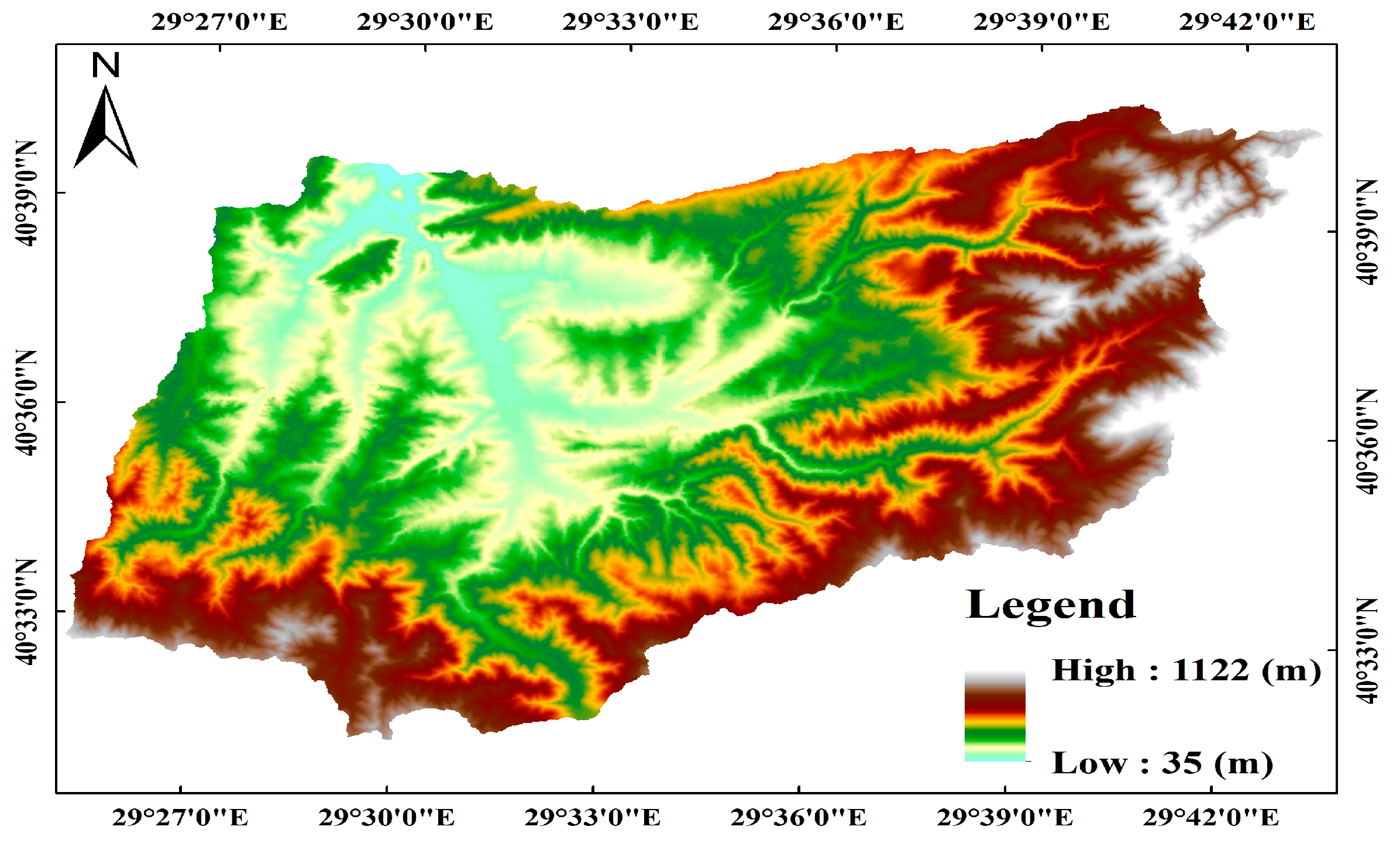
The Ayazma river basin is located in the Marmara region of Turkey between latitudes 40°32′41″–40°39′37″ N and longitudes 29°25′13″–29°43′10″ E. It has a surface area of approximately 267.93 km2 (Figure 1). The basin is surrounded by the Samanlı Mountains, which extend in the east–west direction and form a continuous mass, and there are low alluvial areas in the interior region. The topography of the basin is rugged, with a maximum altitude of 1122 m in the south and 35 m in the interior. The basin mostly consists of agricultural lands where grains, fruits and vegetables are grown. There are some urban settlements in the basin. The largest of these is the town of Karamürsel with a population of approximately 59,000. A transitional climate prevails in the basin between the Mediterranean climate and the Black Sea climate. The annual average precipitation in the basin is approximately 750 mm, and the annual average temperature is around 14 °C. The Yalak river, which is the main water resource of the basin, is approximately 40 km long with an annual average flow rate of 2.51 m3/s at its outlet to the Marmara Sea. There are several reservoirs built on the river for irrigation, drinking and domestic use.
2.2. Data
The observed daily flows were obtained from a stream gauge (D02A041) at the basin outlet (Figure 1) operated by the Turkish State Hydraulic Works (https://www.dsi.gov.tr/Sayfa/Detay/744; accessed on 6 September 2022). Historical data available from 1998 to 2015 were utilized for calibration and validation of the HBV-Light hydrological model.
Since there is no meteorology station within the basin, meteorological data were obtained from different databases as grid data. Daily precipitation and temperature (maximum and minimum) were downloaded from GIOVANNI interface (https://giovanni.gsfc.nasa.gov/giovanni/; accessed on 6 September 2022), while wind speed, solar radiation and relative humidity data were taken from POWER Data Access Viewer (https://power.larc.nasa.gov/data-access-viewer/; accessed on 6 September 2022). Two grids were determined within the basin and their centers were taken as points (i.e., Grid_1 and Grid_2 in Figure 1). Bias correction in the climate data was performed with the CMhdy software package.
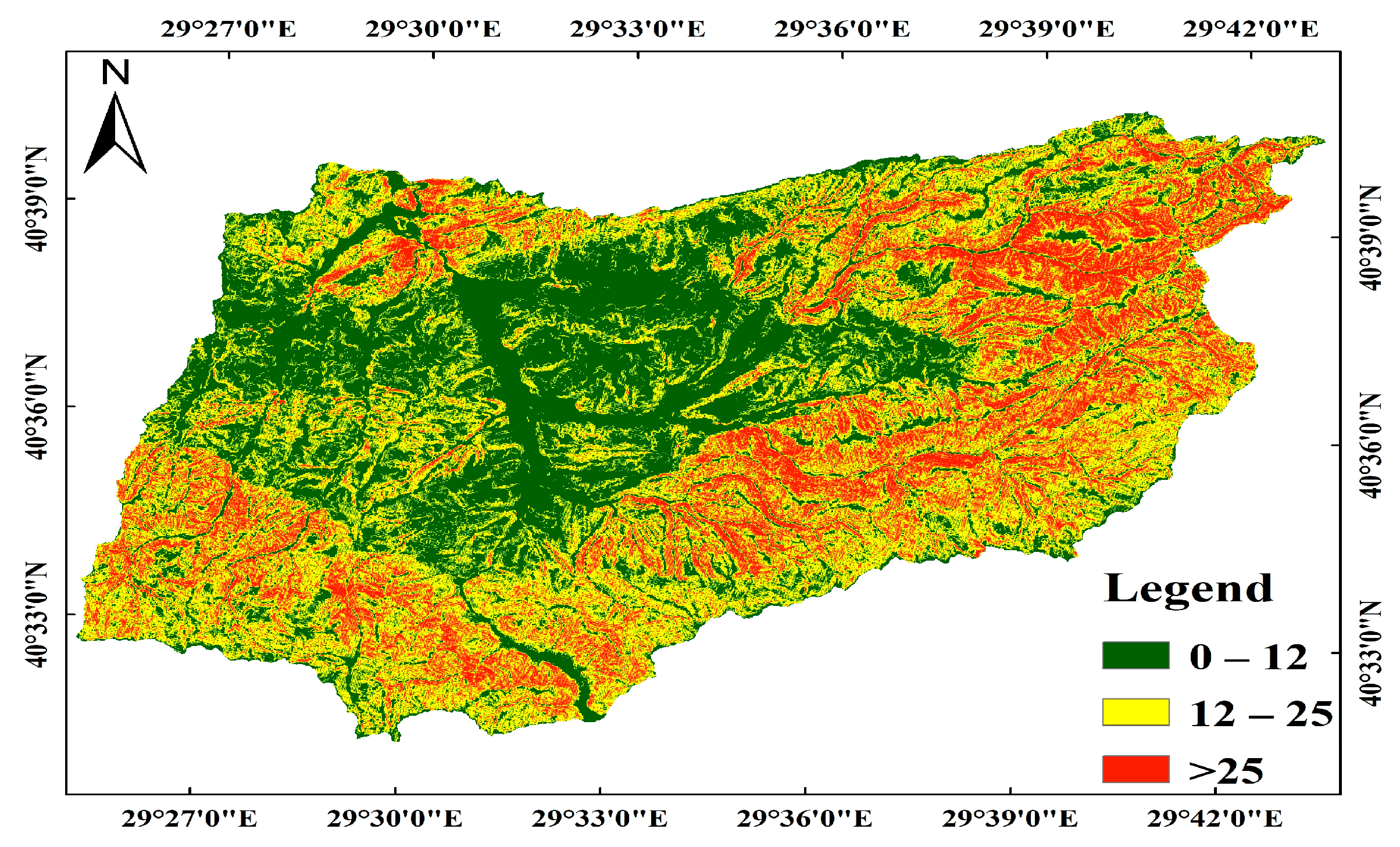
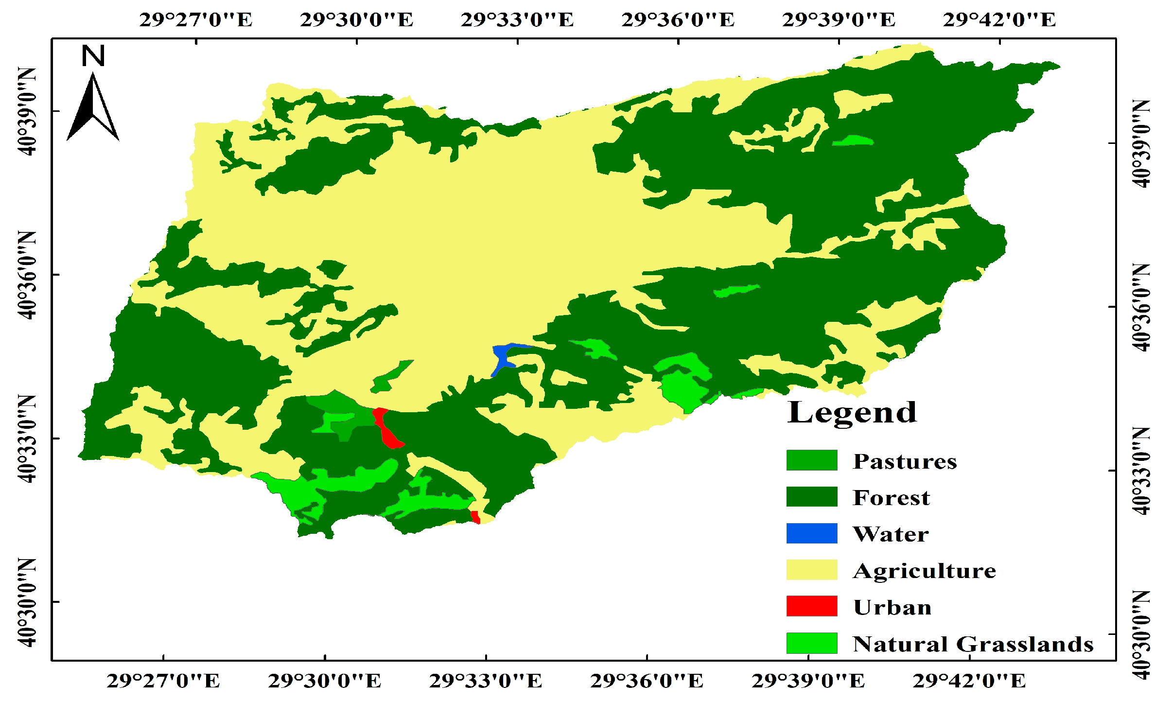
The DEM of the basin (Figure 2) was constructed using the data obtained from the Shuttle Radar Topography Mission (SRTM) database at 30 m spatial resolution (https://portal.opentopography.org/raster?opentopoID=OTSRTM.082015.4326.1; accessed on 1 October 2022). The slope map (Figure 3) was created from the DEM data. The land use/land cover (LU/LC) map (Figure 4) was derived from the CORINE database with a scale of 1:100,000 (https://www.eea.europa.eu/publications/COR0-landcover; accessed on 1 October 2022). The soil data were retrieved from the FAO/UNESCO database with a scale of 1:5,000,000 (https://www.fao.org/soils-portal/data-hub/soil-maps-and-databases/faounesco-soil-map-of-the-world/en/; accessed on 1 October 2022). The dominant soil type in the basin is Lo91-2bc-3208 (D group, medium-textured, loamy Orthic Luvisols).
2.3. Climate Models
For this study, model outputs from three RCMs (CNRM-CM5/RCA4, EC-EARTH/RACMO22E and NorESM1-M/HIRHAM5) from 2006 to 2100 were downloaded from CORDEX-EURO11 for RCP4.5 and RCP8.5 scenarios (Table 1). Bias correction was performed with the CMhyd (Climate Model data for hydrological modelling) tool using the historical data between 1970 and 2005.
2.4. The Mann–Kendall Trend Test
The Mann–Kendall (M-K) trend test is often used to investigate the statistical significance of increases or decreases in hydro-meteorological time series [31]. For the M-K trend test, the S statistic obtained by Equations (1) and (2) is used.
where xi and xj are the ordinal values of the variable under consideration, n is the data length. The S statistic is approximately normally distributed, and its mean is zero. In a considered data series, a positive S value indicates an increasing trend, a negative S value indicates a decreasing trend, while a zero value indicates no trend. The null hypothesis (Ho) states that there is no trend in the data series. The S variance statistic calculated by Equation (3) is asymptotically normal [32].
In cases where the number of data is more than 10, the Z statistic is calculated using Equation (4).
The existence of a statistically significant trend is determined by the Z statistic. A positive Z value indicates an increasing trend, and a negative value indicates a decreasing trend. Z is normally distributed. If the absolute value of the Z statistic is greater than Z1- α/2 for a determined α significance level, the Ho hypothesis is rejected (trend exists), otherwise the Ho hypothesis is accepted (no trend). Here, the Z1- α/2 value is obtained from the standard normal cumulative distribution tables.
2.5. The Standardized Precipitation–Evapotranspiration Index (SPEI)
The SPEI method was developed in 2010 to identify, detect and monitor drought events. As one of the drought indices recommended for use worldwide by the World Meteorological Organization, the method is also effective in explaining the effects and consequences of global warming on arid conditions. It combines the sensitivity of the Palmer Drought Severity Index to changes in evaporation demand, as well as the multi-time scale feature and simple calculation of the Standardized Precipitation Index (SPI) [33,34]. For an accurate assessment of drought with global warming, the increase in evaporation caused by warming cannot be ignored. Therefore, SPEI is noticeably better than SPI in drought monitoring [35]. Based on the principle of water balance, SPEI is calculated using the difference (D) between precipitation (P) and potential evapotranspiration (PET) to evaluate arid and humid conditions. Here, D is the excessive or scarce water for a selected period (i) and it can be calculated mathematically by Equation (5). In this study, PET values were obtained by using the Thornthwaite method [36], which requires monthly average temperature and latitude data of the selected meteorology station.
SPEI can be calculated using the same steps as in SPI and is obtained by converting the log-logistic distribution to the standard normal distribution [37]. The three-parameter log-logistical probability density function given in Equation (6) is used to fit D series obtained by Equation (6) [38].
where are scale, shape and origin parameters, respectively. The cumulative distribution function F(x) for a given time scale is given in Equation (7).
SPEI values can be determined as standardized values of F(x) using Equations (8) and (9) with a mean of zero and a standard deviation of 1.0 [1,5].
where p is the probability of exceeding a determined value of D (p = 1 − F(x)). If p > 0.5, it is replaced by (1-p) and the sign of the calculated SPEI is reversed. The parameters are given as = 2.522, = 0.803, = 0.010, = 1.433, = 0.189 and = 0.001. SPEI values with a mean value of zero and a standard deviation of 1 are obtained. In dry spells, an SPEI of −0.99 to 0.99 is considered near normal, −1.0 to −1.49 moderate drought, −1.5 to −1.99 severe drought and −2.0 or less extreme drought.
2.6. Hydrological Models
Hydrological models have been utilized for simulation and/or prediction of hydrological system responses, such as discharge, floods and droughts in river basins [39,40]. There are various types of hydrological models with different capabilities. Among these, HEC-HMS (The Hydrologic Modeling System) [https://www.hec.usace.army.mil/software/hec-hms/; accessed on 10 October 2022], SWMM (Storm Water Management Model) [https://www.epa.gov/water-research/storm-water-management-model-swmm; accessed on 20 January 2023], SWAT (Soil and Water Assessment Tool) [41], HBV-Light (Hydrologiska Byråns Vattenbalansavdelning) [https://www.geo.uzh.ch/en/units/h2k/Services/HBV-Model.html; accessed on 10 October 2022], SWIM (Soil and Water Integrated Model) [42] and HYPE (Hydrological Predictions for the Environment) [43], are widely used for hydrological modelling and various water resource management tasks in river basins.
2.7. The HBV-Light Model
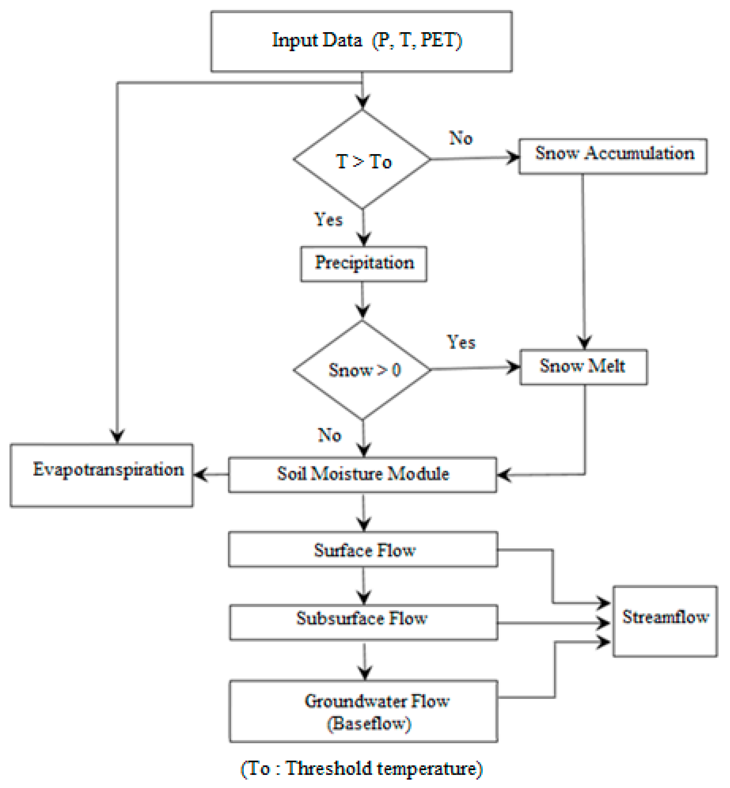
The HBV model was originally developed at the Swedish Meteorology and Hydrology Institute (SMHI) [47,48,49]. It is a conceptual and semi-distributed hydrological model for flow simulation that allows dividing the watershed into sub-basins, elevation and vegetation zones. It requires relatively little input data (Table 2) and has been successfully applied to many river basins in Sweden and other countries [50].
It is relatively simple to perform a hydrological simulation with the HBV-Light model. For this purpose, first the main input data file (i.e., PTQ file) is prepared as a text file. In this file, precipitation (P) is given in mm/day or mm/month (if the model is run monthly), while average air temperatures (T) are tabulated in °C and observed flows are provided in mm/day. Two additional input files (called T_Mean and Evap) are needed for monthly average temperature and potential evapotranspiration data, respectively. The monthly potential evapotranspiration (PET) was estimated by the Thornthwaite method. The schematically summarized conceptual physics of the HBV model flow transform module is presented in Figure 5.
The overall water balance of the HBV model is given by Equation (10) below.
where P is precipitation, E is evapotranspiration, Q is discharge, SP is the amount of snow, SM is soil moisture, UZ is water stored in unsaturated zone, LZ is water stored in saturated zone and VL is water stored in lakes or reservoirs in the basin.
2.8. Hydrological Model Calibration and Validation
Calibration is the process of adjusting model parameters at reasonable intervals until the simulated results are close enough to the observed values [52]. On the other hand, validation is the act of ensuring that the calibrated model reproduces a set of observations or can predict future conditions without any additional adjustments to the parameters [53]. In this study, the meteorological and streamflow data from 1988 to 2015 (17 years of data) are divided into 3 different time periods: (i) 1998–1999 for warm up (i.e., an adjustment process for the model to reach an optimal state [54]), (ii) 1999–2009 for calibration and (iii) 2009–2015 for verification of the selected hydrological model.
2.8.1. The HBV-Light Model
The HBV-Light model has different calibration and optimization tools such as Monto Carlo Studies, Batch Studies and GAP Optimization. In this study, the GAP Optimization tool was chosen for both calibration and validation. The Nash–Sutcliffe Model Efficiency (NSE) was selected as the main objective function. The study area was divided into three elevation bands to achieve relatively reasonable model outputs (Table 3).
2.8.2. Goodness of Fit Tests
To obtain the best fit and a satisfactory modeling result, the accuracy of the outputs and the process simulation need to be examined for calibration [55]. There are various model performance measures (PMs) with different criteria. The following PMs were employed for the hydrological model outputs in this study:
- -
- Nash–Sutcliffe Model Efficiency Coefficient (NSE): NSE is a normalized statistic that determines the relative magnitude of residual variance (i.e., noise) compared to the measured data variance (i.e., information). It varies between −∞ and 1 and is calculated by the relationship given in Equation (11) [56].
- -
- Coefficient of Determination (R2): Ranging from 0 to 1, R2 defines the ratio of variance in the measured data described by the model (Equation (12)). Higher values indicate less error variance, and typically values greater than 0.5 are considered acceptable [55].where is the observed flow, is the simulated flow, is the average observed flow, is the average simulated flow and n is the total number of observations.
It is recommended that model performance can be judged satisfactory for flow simulations if daily, monthly or annual R2 > 0.60 and NSE > 0.50 for watershed-scale models [55].
- -
- Root Mean Squared Error (RMSE): RMSE is one of the commonly used error index statistics. It expresses the average magnitude of the differences between the observation and model values (Equation (13)). For the results to be acceptable, the RMSE is expected to be close to 0 and smaller than the observation standard deviation [55].
The flowchart of the study is given in Figure 6, which summarizes the steps followed in this study.
3. Results
3.1. Precipitation and Temperature Projections
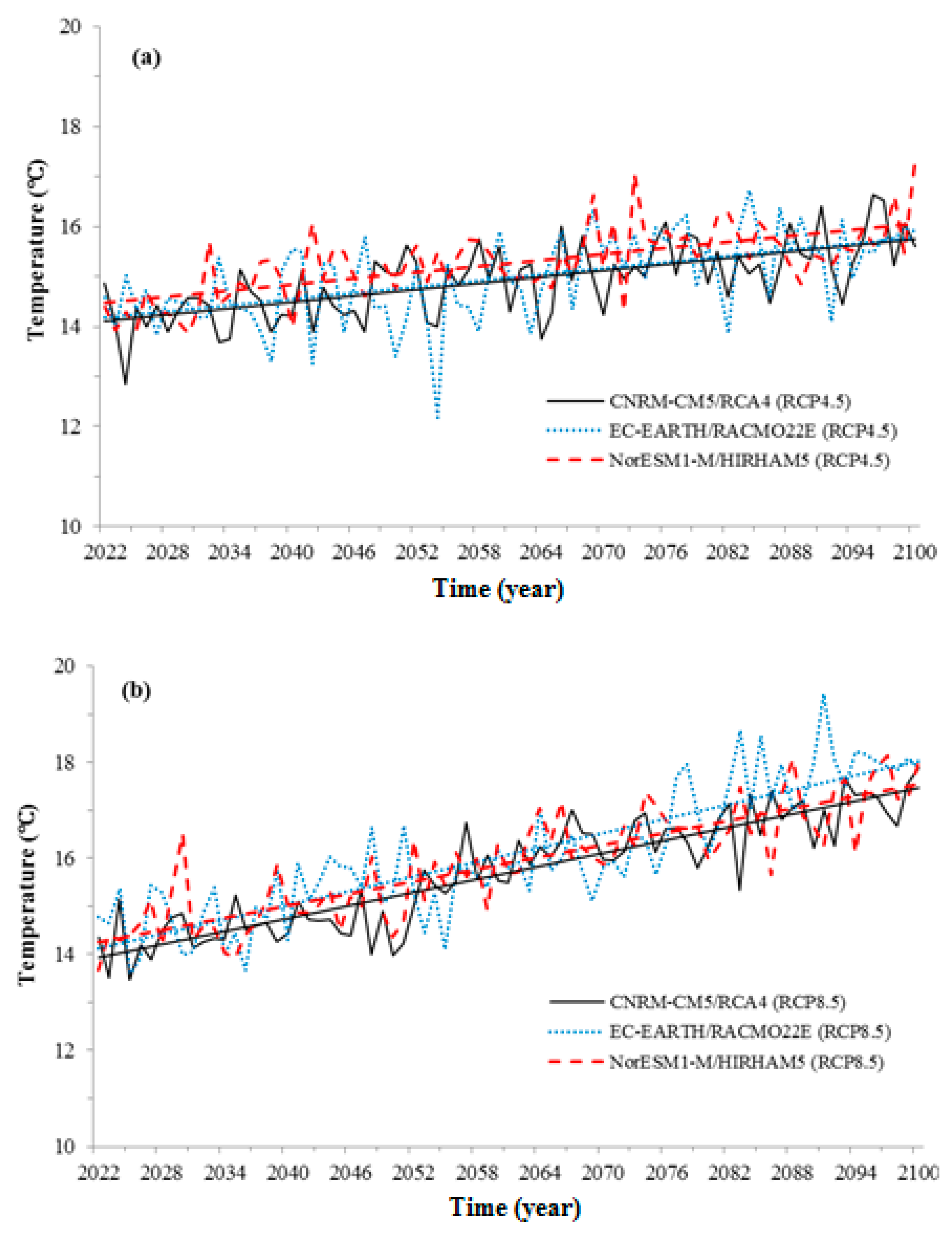
The time series of spatially averaged annual precipitation and mean annual temperature from the selected RCMs are shown in Figure 7 and Figure 8, respectively. The linear trend lines are also displayed on the figures. As shown in Figure 7, for both RCP scenarios, EC-EARTH/RACMO22E appears to produce relatively higher precipitation, while NorESM1-M/HIRHAM5 seems to predict relatively lower precipitation for the period 2022–2100. Compared to the reference period (1970–2005), the increase in annual mean precipitation is calculated to range from 22 to 227 mm for the RCP4.5 scenario and 32 to 222 mm for the RCP8.5 scenario. On the other hand, temperature projections have visible upward trends for all RCMs. Based on the reference period, it is determined that the annual average temperature increase will be around 1.4–1.8 °C for the RCP4.5 scenario and 2.2–2.6 °C for the RCP8.5 scenario until 2100.
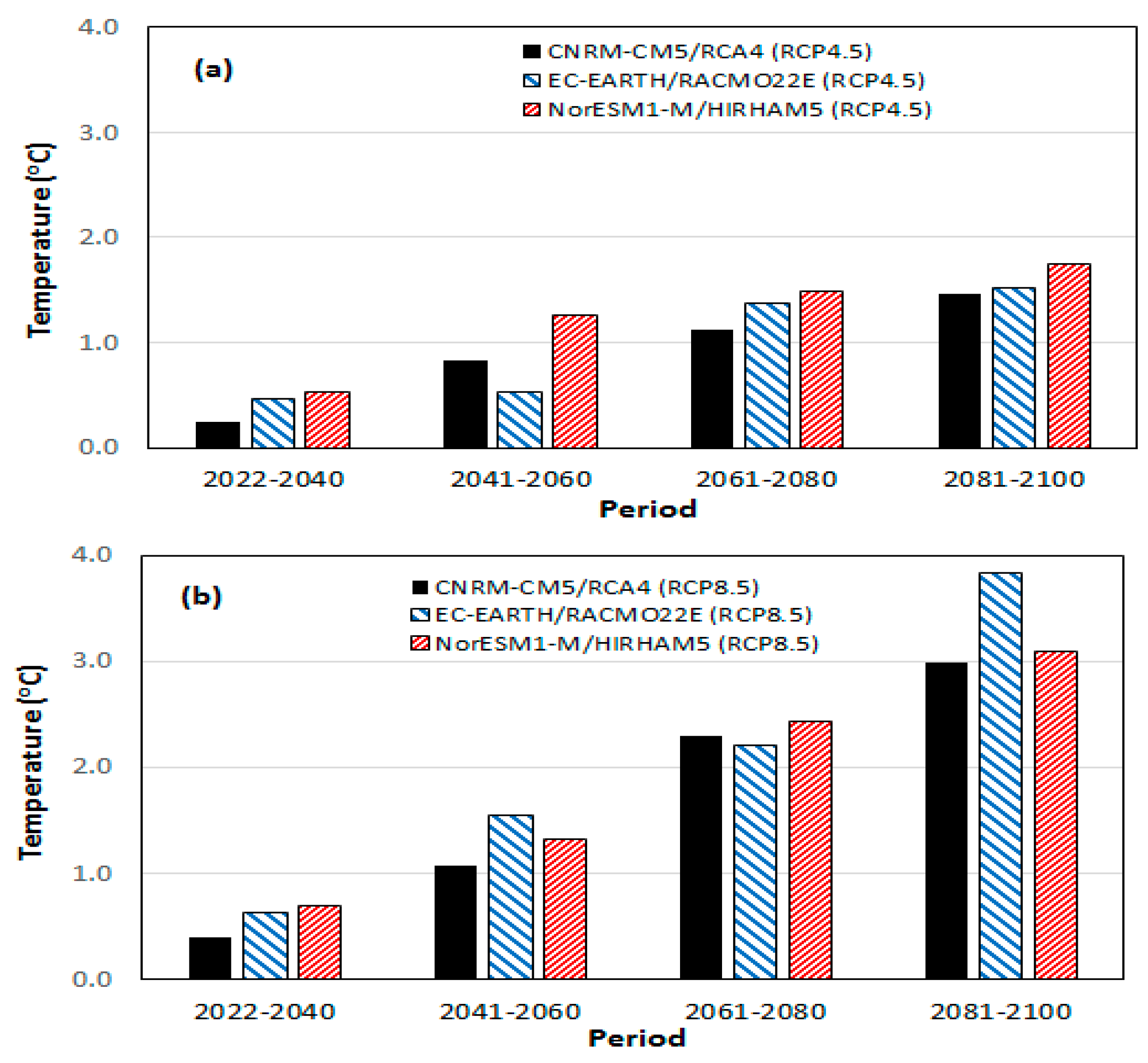
Precipitation and temperature anomalies calculated for 20-year periods are shown in Figure 9 and Figure 10, respectively. According to Figure 9, the distribution of precipitation anomalies in the selected periods for both RCP scenarios is very similar. The CNRM-CM5/RCA4 and EC-EARTH/RACMO22E outputs appear to cause relatively high positive anomalies ranging from 100 to 300 mm. Figure 10 indicates relative increases in temperature anomalies during the study period for both RCP scenarios. Here, all three RCM outputs appear to produce positive anomalies close to each other in each selected period. For the RCP8.5 scenario, the temperature anomalies after the year 2060 are found to be higher than 2 °C.
3.2. The Mann–Kendall Trend Test Results
In this study, the Mann–Kendall trend test was performed with the RStudio software tool for projection data between 2022 and 2100. The trend results for annual precipitation and mean annual temperature data are presented in Table 4 and Table 5, respectively. As shown here, precipitations have statistically insignificant trends, while temperatures have statistically significant upward trends for both RCP scenarios at the 5% significance level (i.e., p = 0.05).
3.3. Meteorological Drought Assessment with the SPEI Method
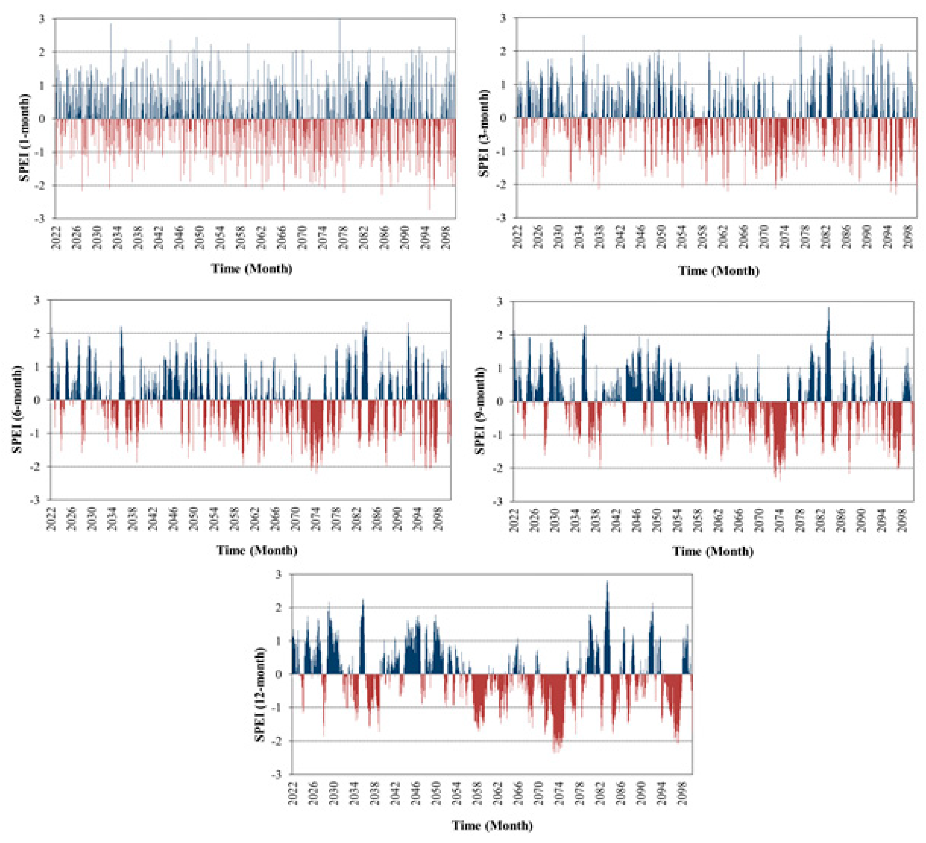
The temporal characteristics of meteorological droughts for the period 2022–2100 in the basin were investigated by SPEI method at 1-, 3-, 6-, 9- and 12-month timescales. For this purpose, monthly CNRM-CM5/RCA4 (RCP8.5) precipitation and temperature projections with the highest Z statistic values were selected. The time series of SPEI calculated with the RStudio software tool for the selected time scales are presented in Figure 11. It is shown here that the frequency of dry periods is relatively high in short time scales and decreases as the times scale increases. There appears to be a significant increase in drought intensities and drought durations at time scales greater than 6 months after 2056. The long-term average value of drought intensities for the SPEI—12-month scale is calculated as −0.21 for the 2022–2055 period and −0.58 for the 2056–2100 period. The maximum drought intensity is found to be −2.4 during the 2071–2076 drought period.
3.4. Calibration and Validation of the HBV-Light Model
Calibration and verification of HBV-Light model was carried out with the use of daily streamflow data. The model results are shown on a monthly basis in Figure 12. The figure shows that the model the simulation results are comparable to the observations. The timing of peak flows is generally good, but some peak flows are underestimated by the model. The performance measures for calibration and validation are presented in Table 6. According to these results, the performance of the hydrological model is found to be satisfactory with relatively high values for NSE (0.73 and 0.67 for calibration and validation, respectively) and R2 (0.73 and 0.71 for calibration and validation, respectively), and also relatively low values for RMSE (4.36 and 5.94 for calibration and validation, respectively).
3.5. Hydrological Model Simulations for Future Climate Change
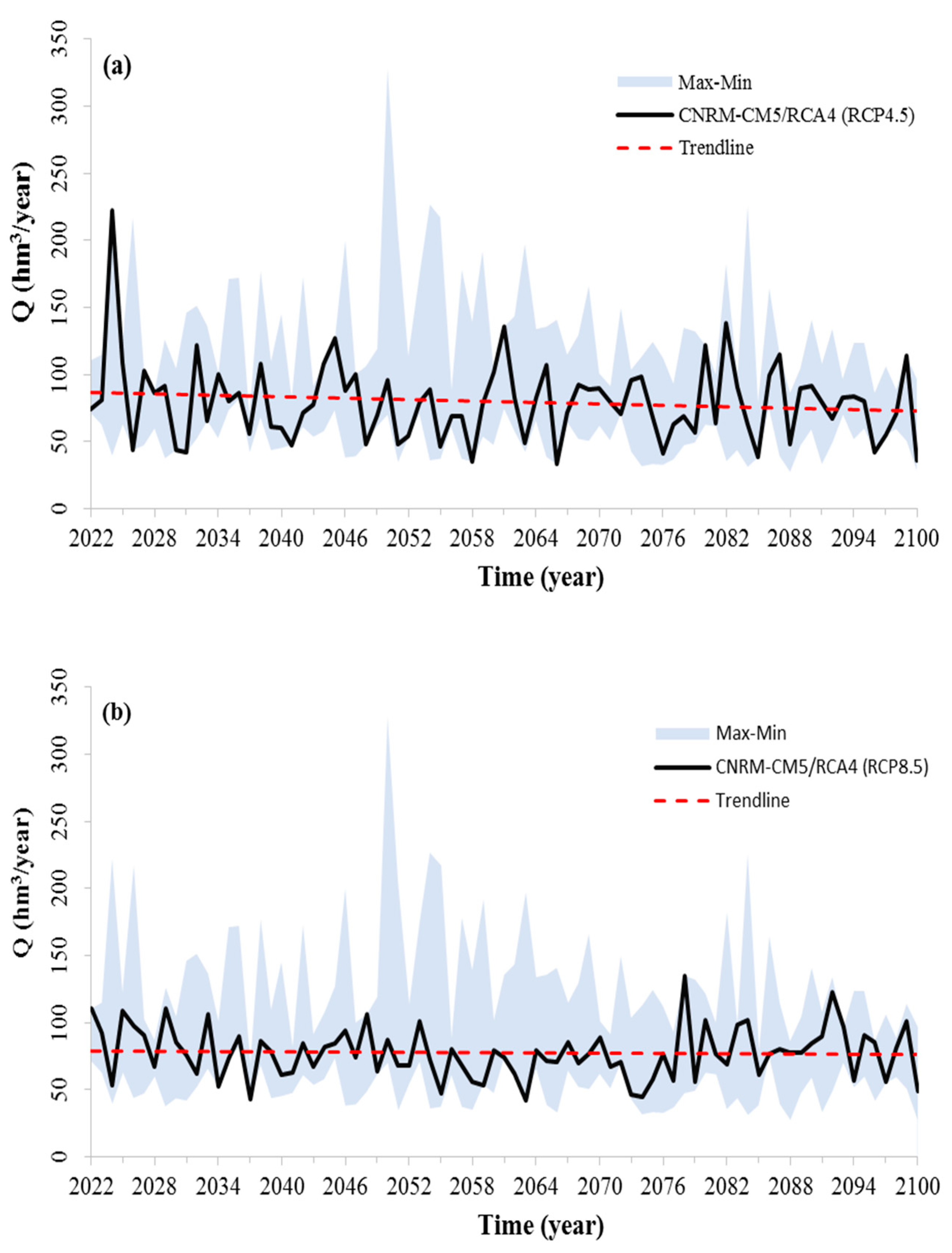
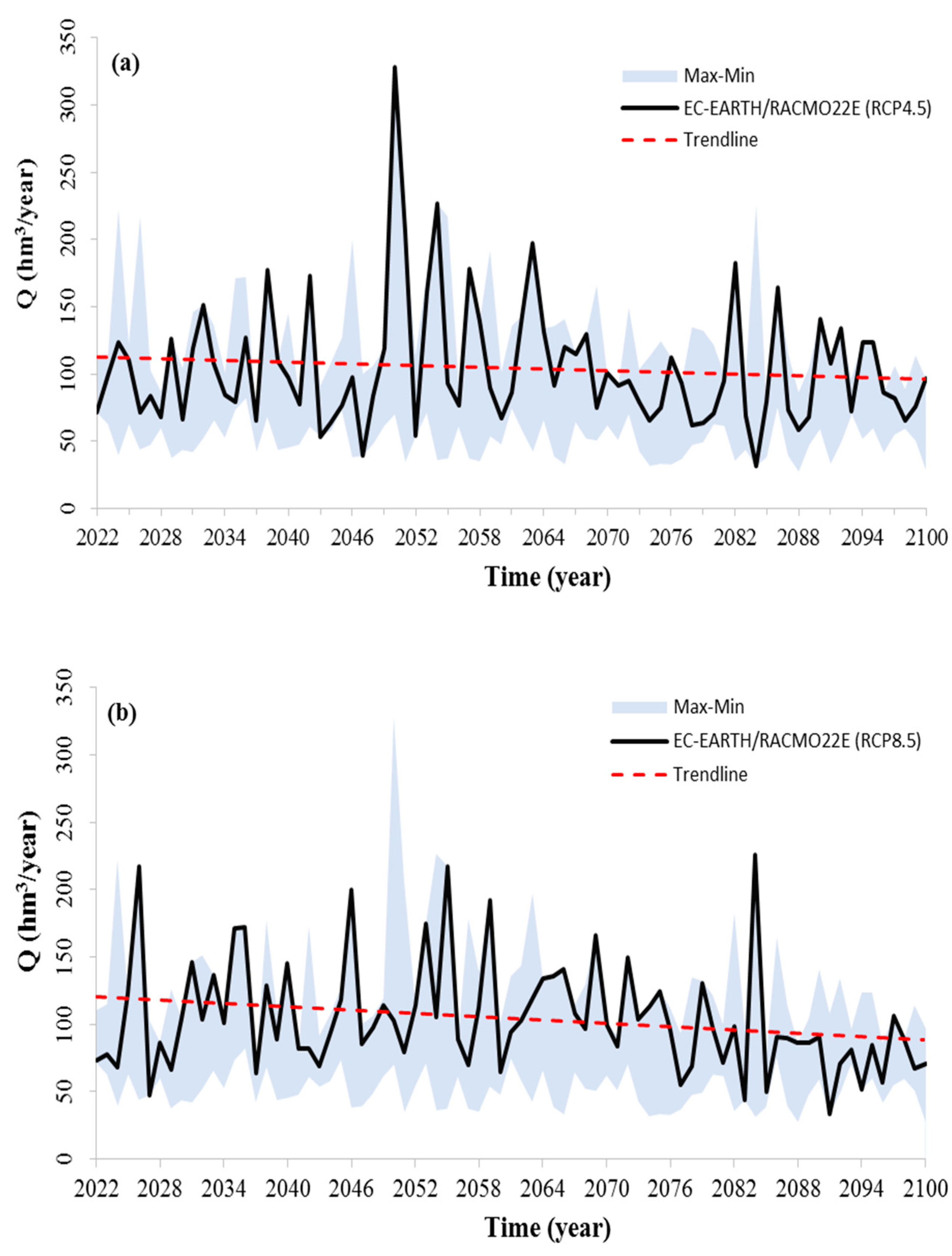
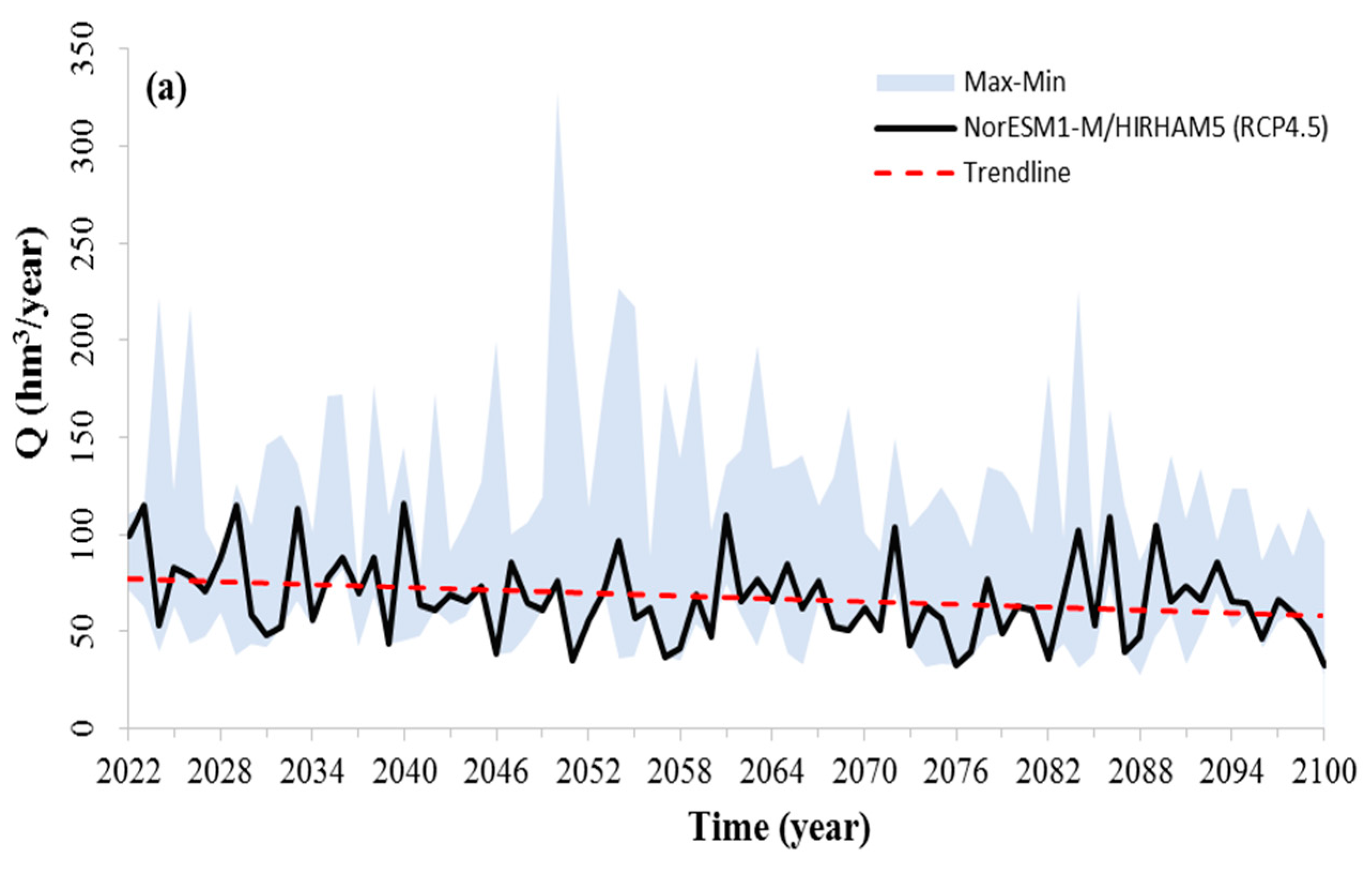
Hydrological model estimates of river flows in the study basin were produced for the period 2022–2100. The hydrological model was driven by the regional climate change outputs obtained from CNRM-CM5/ RCA4, EC-EARTH/ RACMO22E and NorESM1-M/ HIRHAM5 for both RCP4.5 and RCP8.5 emission scenarios. The time series of model simulations with linear trend lines are displayed in Figure 13, Figure 14 and Figure 15. Here, the maximum and minimum output ranges of all models and emission scenarios are also given for comparison. As the figures indicate, all streamflow simulations have decreasing trends over the simulation period. For all RCMs, the streamflow peaks obtained with the RCP8.5 scenario are generally lower than those obtained with the RCP4.5 scenario. The hydrological model seemed to simulate relatively larger peaks with EC-EARTH/RACMO22E outputs for both RCP scenarios as a result of relatively high precipitation projections (see Figure 7 and Figure 9).
The long-term basin-scale averages of simulated (Qsim) and observed streamflows (Qobs) are given in Table 7 for comparison. As shown in the table, these values are very close to each other for both RCP scenarios in all RCMs. It is determined that the simulation averages of CNRM-CM5/RCA4 and NorESM1-M/HIRHAM5 are slightly lower than the observation average (approximately 2 to 10%). On the other hand, the EC-EARTH/RACMO22E value is relatively higher up to 32%. Annual averages of basin-scale streamflow simulations and anomalies for the 20-year periods are given in Table 8. According to the table, streamflow simulations and anomalies generally tend to decline after the middle of the century.
4. Discussion
4.1. Analysis of Climate Model Projections
In this study, temporal changes in precipitation and temperature data projected by the selected RCMs in the Ayazma river basin were evaluated on an annual basis for the period 2022–2100. Annual precipitations generally appear to have a slight upward trend, except for one case with the RCP4.5 scenario. Compared with the reference period, positive anomalies ranging from 22 to 227 mm are obtained for all RCMs. Average annual temperatures have a significant upward trend for all climate models and scenarios with increases of up to 1.8 and 2.6 °C for the RCP4.5 and RCP8.5 scenarios, respectively. Precipitation and temperature anomalies are evaluated for the 20-year periods. The precipitation projections from CNRM-CM5/RCA4 and EC-EARTH/RACMO22E produce relatively high positive anomalies ranging between 100 and 300 mm during the entire study period. The temperature projections from all three RCMs caused relatively high positive anomalies above 2 °C for the periods 2061–-2080 and 2081–2100. The trend test results indicate that annual precipitations for the period 2022–2100 have statistically insignificant trends in all RCMs. On the other hand, the annual average temperatures have statistically significant trends at the 5% significance level for both RCP scenarios in all RCMs. It is noted that the results of this study are consistent with the findings of a recent study conducted in the Marmara region, which also includes the Ayazma basin [17]. Although different climate model outputs were used in these studies, it was found that similar trends and anomalies were obtained for precipitation and temperature projections.
4.2. Assessment of Meteorological Droughts
The meteorological drought analysis with the SPEI method shows that the frequency of dry periods is relatively high at short time scales but decreases with increasing time scale. It is seen that both drought intensities and durations increase at time scales greater than 6 months in the 2056–2100 period. This can be attributed to an increase in evapotranspiration resulted from relatively high temperatures in this period. Significant drought events for the years 2056–2060, 2071–2076 and 2094–2098 are identified in the basin at the SPEI—12-month scale (see Figure 11).
4.3. Hydrological Modelling
The performance of the HBV-Light model for calibration and validation was determined satisfactory, with relatively high values for NSE and R2 and relatively low values for RMSE. The streamflow projections obtained with the HBV-Light model are found to have decreasing trends for the years 2022–2100, mainly due to increasing temperatures (see Figure 8 and Figure 10). It is found that the RCM outputs with the RCP8.5 scenario generally produce lower streamflow peaks than the RCP4.5 scenario due to higher emission. The effect of relatively high precipitation projections is evident in the simulations of the relatively larger peaks obtained with the EC-EARTH/RACMO22E outputs for both RCP scenarios. Compared to the reference period (1988–2015), streamflow simulations obtained with the CNRM-CM5/RCA4 and NorESM1-M/HIRHAM5 outputs have mean values slightly lower than observations. On the other hand, the EC-EARTH/RACMO22E outputs produced relatively higher mean values than observations. Annual averages of basin-scale streamflow simulations calculated for the 20-year periods are found to generally decrease after the period 2040–2060. This is mainly due to the increase in temperature anomalies towards the end of the century. The hydrological model results presented here seem to be generally consistent with the streamflow simulations obtained for the Marmara region in [17], which shows that there are certain decreases in streamflow projections across the region after mid-century.
5. Conclusions
This study presented an assessment of climate change effects on streamflow in the Ayazma river basin (a small basin in the Marmara region of Turkey) using the HBV-Light hydrological model. For this purpose, RCM outputs from CNRM-CM5/RCA4, EC-EARTH/RACMO22E and NorESM1-M/HIRHAM5 (with RCP45 and RCP85 emission scenarios) were used to run the model for the period 2022–2100. The evaluation of RCM outputs reveals that precipitation and temperature projections show high temporal variability. The Mann–Kendall trend test indicates statistically insignificant upward and downward trends in precipitation projections and statistically significant upward trends in temperature projections at the selected significance level (p = 0.05) over the study period. The SPEI method for the RCP8.5 scenario revealed an increase in drought frequencies and durations after mid-century due to annual average temperature increases of more than 2 °C. The HBV-Light model produced streamflow estimates for future climate change scenarios in the basin. The hydrological model simulations show decreasing trends in streamflow for all RCMs over the period 2022–2100. This can be attributed to relatively high increases in temperature and, hence, evapotranspiration in the basin during this period. The impact of the emission scenario on streamflow estimates can be seen in the model prediction of flow peaks. In fact, the flow peaks obtained for the RCP8.5 scenario are generally lower than those obtained for the RCP4.5 scenario. The streamflow simulations produced with EC-EARTH/RACMO22E outputs are found to have relatively larger peaks for both RCP scenarios due to relatively high precipitation forecasts. The hydrological model outputs indicate that the streamflow projections obtained with the CNRM-CM5/RCA4 and NorESM1-M/HIRHAM5 outputs have a slightly lower mean value than the observations, while the streamflow projections with the EC-EARTH/RACMO22E outputs have a relatively larger mean value. Overall, the results of this study were found to be generally consistent with the findings of a study conducted in 2016 in the Marmara region, which includes the Ayazma basin.
This study is beneficial for the management of the Ayazma river basin under future climate changes. Streamflow, which is the main water resource in the basin, is primarily used for agricultural irrigation, drinking and domestic use. Therefore, it is necessary to evaluate the impact of climate change on streamflow in the basin for a sustainable development and climate change adaptation options. The findings obtained from this study can provide useful information to decision makers about the implementation of climate change adaptation options in this basin. For further studies, climate model outputs from other GCMs can be utilized for comparison. The efficiency of hydrological modeling of streamflow under future climate change scenarios in the Ayazma river basin can be further tested using different models such as the SWMM model.
Author Contributions
Conceptualization, K.H.S., R.S., O.Y., G.A., M.G. and J.K.; methodology, K.H.S., R.S., O.Y., G.A., M.G. and J.K.; software, K.H.S., R.S. and G.A.; validation, K.H.S. and R.S.; formal analysis, K.H.S. and R.S.; investigation, K.H.S., R.S., O.Y., G.A., M.G. and J.K.; resources, K.H.S., R.S., G.A., M.G. and J.K.; data curation, G.A.; writing—original draft preparation, K.H.S. and R.S.; writing—review and editing, O.Y. and J.K.; visualization, K.H.S. and R.S.; supervision, O.Y.; project administration, K.H.S. All authors have read and agreed to the published version of the manuscript.
Funding
This research received no external funding.
Data Availability Statement
The meteorological data presented in this study are available at https://giovanni.gsfc.nasa.gov/giovanni/; accessed on 6 September 2022), discharge data are available at https://www.dsi.gov.tr/Sayfa/Detay/744; accessed on 6 September 2022) and the climate model data are available at https://www.euro-cordex.net/060378/index.php.en; accessed on 15 January 2022).
Conflicts of Interest
The authors declare no conflict of interest.
References
- Yilmaz, A.G.; Imteaz, M.A. Impact of climate change on runoff in the upper part of the Euphrates basin. Hydrol. Sci. J. 2011, 56, 1265–1279. [Google Scholar] [CrossRef]
- Selek, B.; Tuncok, I.K. Effects of climate change on surface water management of Seyhan basin, Turkey. Environ. Ecol. Stat. 2014, 21, 391–409. [Google Scholar] [CrossRef]
- Zhou, X.; Zhang, Y.; Yang, Y. Comparison of two approaches for estimating precipitation elasticity of streamflow in China’s main river basins. Adv. Meteorol. 2015, 2015, 924572. [Google Scholar] [CrossRef]
- Zhang, Y.; Li, H.; Reggiani, P. Climate variability and climate change impacts on land surface, hydrological processes and water management. Water 2019, 11, 1492. [Google Scholar] [CrossRef] [Green Version]
- Wang, H.; Yu, X. Sensitivity analysis of climate on streamflow in north China. Theor. Appl. Climatol. 2015, 119, 391–399. [Google Scholar] [CrossRef]
- Brunner, L.; Lorenz, R.; Zumwald, M.; Knutti, R. Quantifying uncertainty in European climate projections using combined performance-independence weighting. Environ. Res. Lett. 2019, 14, 124010. [Google Scholar] [CrossRef]
- Middelkoop, H.; Daamen, K.; Gellens, D.; Grabs, W.; Kwadijk, J.C.J.; Lang, H.; Parmet, B.W.A.H.; Schädler, B.; Schulla, J.; Wilke, K. Impact of climate change on hydrological regimes and water resources management in the Rhine basin. Clim. Chang. 2001, 49, 105–128. [Google Scholar] [CrossRef]
- Brunner, L.; Pendergrass, A.G.; Lehner, F.; Merrifield, A.L.; Lorenz, R.; Knutti, R. Reduced global warming from CMIP6 projections when weighting models by performance and independence. Earth Syst. Dyn. 2020, 11, 995–1012. [Google Scholar] [CrossRef]
- De Girolamo, A.M.; Bouraoui, F.; Buffagni, A.; Pappagallo, G.; Lo Porto, A. Hydrology under climate change in a temporary river system: Potential impact on water balance and flow regime. River Res. Appl. 2017, 33, 1219–1232. [Google Scholar] [CrossRef]
- Edenhofer, O.; Pichs-Madruga, R.; Sokona, Y.; Farahani, E.; Kadner, S.; Seyboth, K.; Adler, A.; Baum, I.; Brunner, S.; Eickemeier, P.; et al. IPCC, Mitigation of Climate Change. Contribution of Working Group III to the Fifth Assessment Report of the Intergovernmental Panel on Climate Change; Cambridge University Press: Cambridge, UK; New York, NY, USA, 2014. [Google Scholar]
- Gebrechorkos, S.H.; Bernhofer, C.; Hülsmann, S. Climate change impact assessment on the hydrology of a large river basin in Ethiopia using a local-scale climate modelling approach. Sci. Total Environ. 2020, 742, 140504. [Google Scholar] [CrossRef]
- Yang, W.; Andréasson, J.; Graham, L.P.; Olsson, J.; Rosberg, J.; Wetterhall, F. Distribution-based scaling to improve usability of regional climate model projections for hydrological climate change impacts studies. Hydrol. Res. 2010, 41, 211–229. [Google Scholar] [CrossRef]
- Tan, M.L.; Juneng, L.; Tangang, F.T.; Samat, N.; Chan, N.W.; Yusop, Z.; Ngai, S.T. SouthEast Asia HydrO-meteorological droughT (SEA-HOT) framework: A case study in the Kelantan River Basin, Malaysia. Atmos. Res. 2020, 246, 105155. [Google Scholar] [CrossRef]
- Bozkurt, D.; Turuncoglu, U.; Sen, O.L.; Onol, B.; Dalfes, N. Downscaled simulations of the ECHAM5, CCSM3 and HadCM3 global models for the eastern Mediterranean-Black Sea region: Evaluation of the reference period. Clim. Dyn. 2012, 39, 1–19. [Google Scholar] [CrossRef]
- Turkes, M.; Turp, M.T.; An, N.; Ozturk, T.; Kurnaz, M.L. Impacts of Climate Change on Precipitation Climatology and Variability in Turkey. In Water Resources of Turkey; Harmancioglu, N., Altinbilek, D., Eds.; World Water Resources; Springer: Cham, Switzerland, 2020; Volume 2. [Google Scholar] [CrossRef]
- Bozkurt, D.; Sen, O.L. Climate change impacts in the Euphrates–Tigris Basin based on different model and scenario simulations. J. Hydrol. 2013, 480, 149–161. [Google Scholar] [CrossRef]
- The Turkish General Directorate of Water Management (SYGM). Impact of Climate Change on Water Resources Project (In Turkish); The Ministry of Forest and Water Works of Turkey: Ankara, Turkey, 2016. Available online: https://www.tarimorman.gov.tr/SYGM/Belgeler/iklim%20de%C4%9Fi%C5%9Fikli%C4%9Finin%20su%20kaynaklar%C4%B1na%20etkisi/Iklim_NihaiRapor.pdf (accessed on 20 December 2022).
- Gorguner, M.; Kavvas, M.L.; Ishida, K. Assessing the impacts of future climate change on the hydroclimatology of the Gediz Basin in Turkey by using dynamically downscaled CMIP5 projections. Sci. Total Environ. 2019, 648, 481–499. [Google Scholar] [CrossRef]
- Gorguner, M.; Kavvas, M.L. Modeling impacts of future climate change on reservoir storages and irrigation water demands in a Mediterranean basin. Sci. Total Environ. 2020, 748, 141246. [Google Scholar] [CrossRef]
- Yıldırım, Ü.; Güler, C.; Önol, B.; Rode, M.; Jomaa, S. Modelling of the Discharge Response to Climate Change under RCP8.5 Scenario in the Alata River Basin (Mersin, SE Turkey). Water 2021, 13, 483. [Google Scholar] [CrossRef]
- Pilevneli, T.; Capar, G.; Sánchez-Cerdà, C. Investigation of climate change impacts on agricultural production in Turkey using volumetric water footprint approach. Sustain. Prod. Consum. 2023, 35, 605–623. [Google Scholar] [CrossRef]
- Yılmaz, M.; Alp, H.; Tosunoğlu, F.; Aşıkoğlu, Ö.L.; Eriş, E. Impact of climate change on meteorological and hydrological droughts for Upper Coruh Basin, Turkey. Nat. Hazards 2022, 112, 1039–1063. [Google Scholar] [CrossRef]
- Cilek, A.; Berberoglu, S.; Kirkby, M.; Irvine, B.; Donmez, C.; Erdogan, M.A. Erosion modelling in a Mediterranean subcatchment under climate change scenarios using Pan-European Soil Erosion Risk Assessment (PESERA). The International Archives of the Photogrammetry, Remote Sensing and Spatial Information Sciences, Volume XL-7/W3. In Proceedings of the 2015 36th International Symposium on Remote Sensing of Environment, Berlin, Germany, 11–15 May 2015; ISPRS: Hannover, Germany, 2015. [Google Scholar]
- Giorgi, F. Climate change hot-spots. Geophys. Res. Lett. 2006, 33, L08707. [Google Scholar] [CrossRef]
- IPCC. Summary for Policymakers. In Climate Change 2007: The Physical Science Basis. Contribution of Working Group I to the Fourth Assessment Report of the Intergovernmental Panel on Climate Change; Solomon, S., Qin, D., Manning, M., Chen, Z., Marquis, M., Averyt, K., Tignor, M., Miller, H., Eds.; Cambridge University Press: Cambridge, UK; New York, NY, USA, 2007. [Google Scholar]
- Giorgi, F.; Lionello, P. Climate change projections for the Mediterranean region. Glob. Planet. Chang. 2008, 63, 90–104. [Google Scholar] [CrossRef]
- Ciscar, J.C.; Ibarreta, D.R.; Soria, A.R.; Feyen, L. Climate Impacts in Europe: Final Report of the JRC PESETA III; Publications Office of the European Union: Luxembourg, 2018. [Google Scholar]
- The Swedish Meteorological and Hydrological Institute. 2014. Available online: https://www.smhi.se/ (accessed on 10 October 2022).
- van Meijgaard, E.; van Ulft, L.H.; van de Berg, W.J.; Bosveld, F.C.; van den Hurk, B.J.J.M.; Lenderink, G.; Siebesma, A.P. The KNMI Regional Atmospheric Climate Model RACMO Version 2.1; KNMI Technical Report-302; KNMI: De Bilt, Netherland, 2008. [Google Scholar]
- Kotlarski, S.; Keuler, K.; Christensen, O.B.; Colette, A.; Déqué, M.; Gobiet, A.; Goergen, K.; Jacob, D.; Lüthi, D.; Van Meijgaard, E.; et al. Regional climate modeling on European scales: A joint standard evaluation of the EURO-CORDEX RCM ensemble. Geosci. Model Dev. 2014, 7, 1297–1333. [Google Scholar] [CrossRef] [Green Version]
- Hırca, T.; Eryılmaz Türkkan, G.; Niazkar, M. Applications of innovative polygonal trend analyses to precipitation series of Eastern Black Sea Basin, Turkey. Theor. Appl. Climatol. 2022, 147, 651–667. [Google Scholar] [CrossRef]
- Hamed, K.H. Trend detection in hydrologic data: The Mann- Kendall trend test under the scaling hypothesis. J. Hydrol. 2008, 349, 350–363. [Google Scholar] [CrossRef]
- Vicente-Serrano, S.M.; Beguería, S.; López-Moreno, J.I. A multiscalar drought index sensitive to global warming: The standardized precipitation evapotranspiration index. J. Clim. 2010, 23, 1696–1718. [Google Scholar] [CrossRef] [Green Version]
- Tirivarombo, S.; Osupile, D.; Eliasson, P. Drought Monitoring and Analysis: Standardised Precipitation Evapotranspiration Index (SPEI) and Standardised Precipitation Index (SPI). Phys. Chem. Earth Parts A/B/C 2018, 106, 1–10. [Google Scholar] [CrossRef]
- Mathbout, S.; Lopez-Bustins, J.A.; Martin-Vide, J.; Bech, J.; Rodrigo, F.S. Spatial and temporal analysis of drought variability at several time scales in Syria during 1961–2012. Atmos. Res. 2018, 200, 153–168. [Google Scholar] [CrossRef]
- Thornthwaite, C.W. An approach toward a rational classification of climate. Geogr. Rev. 1948, 38, 55–94. [Google Scholar] [CrossRef]
- Kumanlioglu, A.A. Characterizing meteorological and hydrological droughts: A case study of the Gediz river basin, Turkey. Meteorol. Appl. 2020, 27, 1–17. [Google Scholar] [CrossRef]
- Pei, Z.; Fang, S.; Wang, L.; Yang, W. Comparative analysis of drought indicated by the SPI and SPEI at various timescales in Inner Mongolia, China. Water 2020, 12, 1925. [Google Scholar] [CrossRef]
- Arnold, J.G.; Fohrer, N. SWAT2000: Current capabilities and research opportunities in applied watershed modelling. Hydrol. Process. 2005, 19, 563–572. [Google Scholar] [CrossRef]
- Todini, E. Hydrological catchment modelling: Past, present and future. Hydrol. Earth Syst. Sci. 2007, 11, 468–482. [Google Scholar] [CrossRef] [Green Version]
- Arnold, J.G.; Srinivasan, R.; Muttiah, R.S.; Williams, J.R. Large area hydrologic modeling and assessment: Part I. Model development. J. Am. Water Resour. Assoc. (JAWRA) 1998, 34, 73–89. [Google Scholar] [CrossRef]
- Krysanova, V.; Hattermann, F.; Wechsung, F. Development of the ecohydrological model SWIM for regional impact studies and vulnerability assessment. Hydrol. Process. 2005, 19, 763–783. [Google Scholar] [CrossRef]
- Lindström, G.; Pers, C.; Rosberg, J.; Strömqvist, J.; Arheimer, B. Development and testing of the HYPE (Hydrological Predictions for the Environment) water quality model for different spatial scales. Hydrol. Res. 2010, 41, 295–319. [Google Scholar] [CrossRef]
- Nonki, R.M.; Lenouo, A.; Tshimanga, R.M.; Donfack, F.C.; Tchawoua, C. Performance assessment and uncertainty prediction of a daily time-step HBV-Light rainfall-runoff model for the Upper Benue River Basin, Northern Cameroon. J. Hydrol. Reg. Stud. 2021, 36, 100849. [Google Scholar] [CrossRef]
- Maxander, O. The Impact of Different Evapotranspiration Models in Rainfall Runoff Modelling Using HBV-light: A Comparison of Six Different Evapotranspiration Models over Three Catchments in Sweden. Master’s Thesis, Division of Water Resources Engineering, Department of Building and Environmental Technology, Lund University, Lund, Sweden, 2021. [Google Scholar]
- Abebe Temesgen, A. Rainfall-runoff modeling: A comparative analyses: Semi distributed HBV Light and SWAT models in Geba catchment, Upper Tekeze Basin, Ethiopia. Civ. Environ. Res. 2019, 11, 23–33. [Google Scholar]
- Bergström, S. Development and Application of a Conceptual Runoff Model for Scandinavian Catchments; RHO, Report Hydrology and Oceanography; SMHI: Norrköping, Sweden, 1976; Volume 7, p. 162. [Google Scholar]
- Bergström, S. Parametervärden för HBV-modellen i Sverige. Erfarenheter från modelkalibreringar under perioden 1975–1989. SMHI Hydrol. 1990, 28, 36. [Google Scholar]
- Bergström, S. The HBV Model—Its Structure and Applications; RH, Report Hydrology; Swedish Meteorological and Hydrological Institute: Norrköping, Sweden, 1992; Volume 4, p. 32. [Google Scholar]
- Seibert, J.; Vis, M.J.P. Teaching hydrological modeling with a user-friendly catchment-runoff-model software package. Hydrol. Earth Syst. Sci. 2012, 16, 3315–3325. [Google Scholar] [CrossRef] [Green Version]
- Killingtveit, A.; Fosdal, M.L. The River System Simulator—An integrated model system for water resources planning and operation transaction. WIT Trans. Ecol. Environ. 1994, 7, 8. [Google Scholar] [CrossRef]
- Zeckoski, R.W.; Smolen, M.D.; Moriasi, D.N.; Frankenberger, J.R.; Feyereisen, G.W. Hydrologic and water quality terminology as applied to modeling. Transactions of the ASABE 2015, 58, 1619–1635. [Google Scholar] [CrossRef]
- Zheng, C.; Hill, M.C.; Cao, G.; Ma, R. MT3DMS: Model use, calibration, and validation. Trans. ASABE 2012, 55, 1549–1559. [Google Scholar] [CrossRef]
- Kim, K.B.; Kwon, H.H.; Han, D. Exploration of warm-up period in conceptual hydrological modelling. J. Hydrol. 2018, 556, 194–210. [Google Scholar] [CrossRef] [Green Version]
- Moriasi, D.N.; Gitau, M.W.; Pai, N.; Daggupati, P. Hydrologic and water quality models: Performance measures and evaluation criteria. Trans. ASABE 2015, 58, 1763–1785. [Google Scholar] [CrossRef] [Green Version]
- Şen, Z.; Şişman, E.; Kızılöz, B. A new innovative method for model efficiency performance. Water Supply 2022, 22, 589–601. [Google Scholar] [CrossRef]
Figure 1.
Location map of the Ayazma river basin.

Figure 2.
The digital elevation map of the Ayazma river basin.

Figure 3.
The slope map of the Ayazma river basin.

Figure 4.
The land use/land cover map of the Ayazma river basin.

Figure 5.
The HBV model flow transform module [51].
Figure 5.
The HBV model flow transform module [51].

Figure 6.
The flow chart of the study.

Figure 7.
Annual precipitation time series produced by the selected RCMs in the Ayazma river basin with (a) RCP4.5 and (b) RCP8.5.
Figure 7.
Annual precipitation time series produced by the selected RCMs in the Ayazma river basin with (a) RCP4.5 and (b) RCP8.5.

Figure 8.
Mean annual temperature time series produced by the selected RCMs in the Ayazma river basin with (a) RCP4.5 and (b) RCP8.5.
Figure 8.
Mean annual temperature time series produced by the selected RCMs in the Ayazma river basin with (a) RCP4.5 and (b) RCP8.5.

Figure 9.
Precipitation anomalies for the selected periods in the Ayazma river basin with (a) RCP4.5 and (b) RCP8.5.
Figure 9.
Precipitation anomalies for the selected periods in the Ayazma river basin with (a) RCP4.5 and (b) RCP8.5.

Figure 10.
Temperature anomalies for the selected periods in the Ayazma river basin with (a) RCP4.5 and (b) RCP8.5.
Figure 10.
Temperature anomalies for the selected periods in the Ayazma river basin with (a) RCP4.5 and (b) RCP8.5.

Figure 11.
The SPEI time series at 1−, 3−, 6−, 9− and 12−month time scales in the Ayazma river basin between 2022 and 2100.
Figure 11.
The SPEI time series at 1−, 3−, 6−, 9− and 12−month time scales in the Ayazma river basin between 2022 and 2100.

Figure 12.
Comparison of monthly observed and simulated streamflows in the Ayazma river basin with the HBV-Light model ((a): calibration; (b): validation).
Figure 12.
Comparison of monthly observed and simulated streamflows in the Ayazma river basin with the HBV-Light model ((a): calibration; (b): validation).

Figure 13.
Streamflow projections from the HBV-Light model with CNRM-CM5/RCA4 outputs for the period 2022–2100 in the Ayazma river basin ((a): RCP4.5; (b): RCP8.5).
Figure 13.
Streamflow projections from the HBV-Light model with CNRM-CM5/RCA4 outputs for the period 2022–2100 in the Ayazma river basin ((a): RCP4.5; (b): RCP8.5).

Figure 14.
Streamflow projections from the HBV-Light model with EC-EARTH/RACMO22E outputs for the period 2022–2100 in the Ayazma river basin ((a): RCP4.5; (b): RCP8.5).
Figure 14.
Streamflow projections from the HBV-Light model with EC-EARTH/RACMO22E outputs for the period 2022–2100 in the Ayazma river basin ((a): RCP4.5; (b): RCP8.5).

Figure 15.
Streamflow projections from the HBV-Light model with NorESM1-M/HIRHAM5 outputs for the period 2022–2100 in the Ayazma river basin ((a): RCP4.5; (b): RCP8.5).
Figure 15.
Streamflow projections from the HBV-Light model with NorESM1-M/HIRHAM5 outputs for the period 2022–2100 in the Ayazma river basin ((a): RCP4.5; (b): RCP8.5).


Table 1.
The GCMs and RCMs used for the study area.
| GCM | Reference | RCM | Reference | Data Period | ||
|---|---|---|---|---|---|---|
| Observation Period | RCP4.5 Scenario | RCP8.5 Scenario | ||||
| CNRM-CM5 | CNRM, 2014, 2017 | RCA4 | [28] | 1970–2005 | 2006–2100 | 2006–2100 |
| EC-EARTH | EC-EARTH, 2022 | RACMO22E | [29] | 1950–2005 | 2006–2100 | 2006–2100 |
| NorESM1-M | NorESM, 2022 | HIRHAM5 | [30] | 1951–2005 | 2006–2100 | 2006–2100 |
Table 2.
The HBV-Light model parameters.
| Parameter | Description | Range |
|---|---|---|
| TT | Threshold temperature | −2~2 |
| CFMAX | Degree-Δt factor | 4~0.01 |
| SP | Seasonal variability in degree-Δt factor | 0.1~0.001 |
| SFCF | Snowfall correction factor | 0.9~0.2 |
| CFR | Refreezing coefficient | 0.1~0.0001 |
| CWH | Water holding capacity | 0.2~0.0001 |
| FC | Maximum soil moisture storage | 500~50 |
| LP | Soil moisture value above which AET reaches PET | 1~0.3 |
| BETA | Parameter that determines the relative contribution to runoff from rain or snowmelt | 5~0.1 |
| PERC | Threshold parameter | 7~0 |
| UZL | Threshold parameter | 70~0 |
| K0 | Storage (or recession) coefficient 0 | 0.8~0.01 |
| K1 | Storage (or recession) coefficient 1 | 0.5~0.01 |
| K2 | Storage (or recession) coefficient 2 | 0.3~0.001 |
| MAXBAS | Length of triangular weighting function | 3~1 |
| Cet | Potential evaporation correction factor | 0.9~0 |
| PCALT | Increase in precipitation with elevation | 12~6 |
| TCALT | Decrease in temperature with elevation | 0.9~−0.9 |
Table 3.
The selected elevation bands in the Ayazma river basin.
| No | Area (km2) | Elevation (m) | % of Total Area | |||
|---|---|---|---|---|---|---|
| Minimum | Maximum | Mean | Standard Deviation | |||
| 1 | 125.44 | 35.00 | 303.00 | 191.01 | 63.36 | 47 |
| 2 | 85.87 | 304.00 | 541.00 | 415.75 | 68.05 | 32 |
| 3 | 56.62 | 542.00 | 1122.00 | 667.17 | 96.15 | 21 |
| Total | 267.93 | 100 | ||||
Table 4.
Trend analysis results for total monthly precipitations for the period 2022–2100 in the Ayazma river basin.
Table 4.
Trend analysis results for total monthly precipitations for the period 2022–2100 in the Ayazma river basin.
| GCM/RCM | RCP4.5 | RCP8.5 | ||||||
|---|---|---|---|---|---|---|---|---|
| Z | p | Trend Direction | Remark | Z | p | Trend Direction | Remark | |
| CNRM-CM5/RCA4 | 0.54 | 0.58 | + | NS | 1.24 | 0.21 | + | NS |
| EC-EARTH/RACMO22E | 0.19 | 0.84 | + | NS | 0.25 | 0.81 | + | NS |
| NorESM1-M/HIRHAM5 | −0.40 | 0.68 | − | NS | 0.49 | 0.62 | + | NS |
Note(s): NS: Not significant at 5% significance level (p = 0.05).
Table 5.
Trend analysis results for monthly average temperatures for the period 2022–2100 in the Ayazma river basin.
Table 5.
Trend analysis results for monthly average temperatures for the period 2022–2100 in the Ayazma river basin.
| GCM/RCM | RCP4.5 | RCP8.5 | ||||||
|---|---|---|---|---|---|---|---|---|
| Z | p | Trend Direction | Remark | Z | p | Trend Direction | Remark | |
| CNRM-CM5/RCA4 | 6.01 | 0.00 | + | S | 9.23 | 0.00 | + | S |
| EC-EARTH/RACMO22E | 4.96 | 0.00 | + | S | 8.60 | 0.00 | + | S |
| NorESM1-M/HIRHAM5 | 6.32 | 0.00 | + | S | 8.72 | 0.00 | + | S |
Note(s): S: Significant at 5% significance level (p = 0.05).
Table 6.
Streamflow modelling performance measures for the HBV-Light model.
| Performance Measure | Calibration | Validation |
|---|---|---|
| NSE | 0.73 | 0.67 |
| R2 | 0.73 | 0.71 |
| RMSE | 4.36 | 5.94 |
Table 7.
Annual averages of basin-scale streamflow simulations and observations.
| RCM | RCP Scenario | Qsim (hm3/Year) [2022–2100] | Qobs (hm3/Year) [1999–2015] |
|---|---|---|---|
| CNRM-CM5/RCA4 | RCP 4.5 | 79.59 | 79.12 |
| RCP 8.5 | 77.40 | ||
| EC-EARTH/RACMO22E | RCP 4.5 | 104.70 | |
| RCP 8.5 | 104.43 | ||
| NorESM1-M/HIRHAM5 | RCP 4.5 | 67.38 | |
| RCP 8.5 | 65.88 |
Table 8.
Annual averages of basin-scale streamflow simulations and anomalies for the 20-year periods.
Table 8.
Annual averages of basin-scale streamflow simulations and anomalies for the 20-year periods.
| RCM (RCP4.5) | ||||||
| CNRM-CM5/RCA4 | EC-EARTH/RACMO22E | NorESM1-M/HIRHAM5 | ||||
| Period | Flow (m3/s) | Anomaly | Flow (m3/s) | Anomaly | Flow (m3/s) | Anomaly |
| 2022–2040 | 86.16 | 7.04 | 102.08 | 22.96 | 79.60 | 0.48 |
| 2041–2060 | 75.30 | −3.82 | 120.28 | 41.16 | 61.53 | −17.59 |
| 2061–2080 | 79.84 | 0.72 | 99.83 | 20.71 | 64.18 | −14.94 |
| 2081–2100 | 77.41 | −1.71 | 96.48 | 17.36 | 64.83 | −14.29 |
| RCM (RCP8.5) | ||||||
| CNRM-CM5/RCA4 | EC-EARTH/RACMO22E | NorESM1-M/HIRHAM5 | ||||
| Period | Flow (m3/s) | Anomaly | Flow (m3/s) | Anomaly | Flow (m3/s) | Anomaly |
| 2022–2040 | 81.38 | 2.26 | 111.63 | 32.51 | 65.35 | −13.77 |
| 2041–2060 | 75.04 | −4.08 | 113.21 | 34.09 | 68.92 | −10.20 |
| 2061–2080 | 71.74 | −7.38 | 110.98 | 31.86 | 64.20 | −14.92 |
| 2081–2100 | 81.65 | 2.53 | 82.25 | 3.13 | 65.03 | −14.09 |
Disclaimer/Publisher’s Note: The statements, opinions and data contained in all publications are solely those of the individual author(s) and contributor(s) and not of MDPI and/or the editor(s). MDPI and/or the editor(s) disclaim responsibility for any injury to people or property resulting from any ideas, methods, instructions or products referred to in the content. |
© 2023 by the authors. Licensee MDPI, Basel, Switzerland. This article is an open access article distributed under the terms and conditions of the Creative Commons Attribution (CC BY) license (https://creativecommons.org/licenses/by/4.0/).
Share and Cite
MDPI and ACS Style
Seddiqe, K.H.; Sediqi, R.; Yildiz, O.; Akturk, G.; Kostecki, J.; Gortych, M. Effects of Climate Change on Streamflow in the Ayazma River Basin in the Marmara Region of Turkey. Water 2023, 15, 763. https://doi.org/10.3390/w15040763
AMA Style
Seddiqe KH, Sediqi R, Yildiz O, Akturk G, Kostecki J, Gortych M. Effects of Climate Change on Streamflow in the Ayazma River Basin in the Marmara Region of Turkey. Water. 2023; 15(4):763. https://doi.org/10.3390/w15040763
Chicago/Turabian StyleSeddiqe, Khaja Haroon, Rahmatullah Sediqi, Osman Yildiz, Gaye Akturk, Jakub Kostecki, and Marta Gortych. 2023. "Effects of Climate Change on Streamflow in the Ayazma River Basin in the Marmara Region of Turkey" Water 15, no. 4: 763. https://doi.org/10.3390/w15040763
Note that from the first issue of 2016, this journal uses article numbers instead of page numbers. See further details here.