Performance of Machine Learning Techniques for Meteorological Drought Forecasting in the Wadi Mina Basin, Algeria

Abstract

Water resources, land and soil degradation, desertification, agricultural productivity, and food security are all adversely influenced by drought. The prediction of meteorological droughts using the standardized precipitation index (SPI) is crucial for water resource management. The modeling results for SPI at 3, 6, 9, and 12 months are based on five types of machine learning: support vector machine (SVM), additive regression, bagging, random subspace, and random forest. After training, testing, and cross-validation at five folds on sub-basin 1, the results concluded that SVM is the most effective model for predicting SPI for different months (3, 6, 9, and 12). Then, SVM, as the best model, was applied on sub-basin 2 for predicting SPI at different timescales and it achieved satisfactory outcomes. Its performance was validated on sub-basin 2 and satisfactory results were achieved. The suggested model performed better than the other models for estimating drought at sub-basins during the testing phase. The suggested model could be used to predict meteorological drought on several timescales, choose remedial measures for research basin, and assist in the management of sustainable water resources.

1. Introduction

Lack of precipitation during a drought is a complex and cyclical phenomenon that has a negative impact on agricultural and water resources, as well as on society [1,2]. The damage caused by drought is relatively higher than other natural disasters, such as extreme drought in South China, which reduced the area of Honghu Lake and severely impacted tourism, aquaculture, and the public [3]. Similar to this, the 2012 US drought cost over 12 billion USD in economic losses and subsequently raised food prices throughout the world [4]. Future droughts are predicted to be more frequent and more intense due to climate change, urging water resource managers to implement comprehensive risk-mitigation measures [5]. The creeping nature of drought can be beneficial for drought scientists to predict these events in advance [6]. In recent decades, advancements in various drought modeling approaches have been observed, which will ultimately play a critical role in effective drought modeling and drought risk reduction.

Droughts can be characterized as agricultural, meteorological, hydrological, or socioeconomic based on the kind of water insufficiency, such as precipitation, runoff, soil moisture, and water availability, respectively [7]. Among these categories, meteorological drought is the most important; it is barely dependent on precipitation and prolonged meteorological drought results in other drought categories [8]. Several drought indices, including the standardized precipitation index (SPI), Palmer drought severity index, standardized precipitation evapotranspiration index (SPEI), standardized runoff index, etc., have been developed in the past few decades to model meteorological, hydrological, and agricultural drought [5,7]. Standardized drought indices have been utilized often for drought modeling because they are easy to use, flexible, and can estimate drought throughout many periods, with few data requirements [3,9].

It is crucial to anticipate a drought before it occurs, in addition to monitoring it [10]. Despite the fact that predicting droughts is a challenging task owing to the inherent uncertainties and high degree of complexity [11], drought forecasting analysis is essential for supplying pertinent data for drought risk reduction [12]. In hydro-meteorological applications, physical and data-driven models are the most common drought forecasting models [13]. Data-driven models create the strongest link between independent and dependent variables, whereas physical-based models are focused on understanding the real dynamics of a system [14]. The parameter estimation of physical process-based models requires information regarding soil, land use, geography, topography, water abstraction, etc., which is not only difficult to obtain, but also poses difficulties in terms of deviating from a thorough scientific understanding of different physical processes [15]. Because of the drawbacks of physical process-based models, data-driven models are used increasingly frequently in the field of hydrology and water management. Data-driven models such as machine learning models, regression models, and time-series models are commonly used in drought forecasting [5,16].

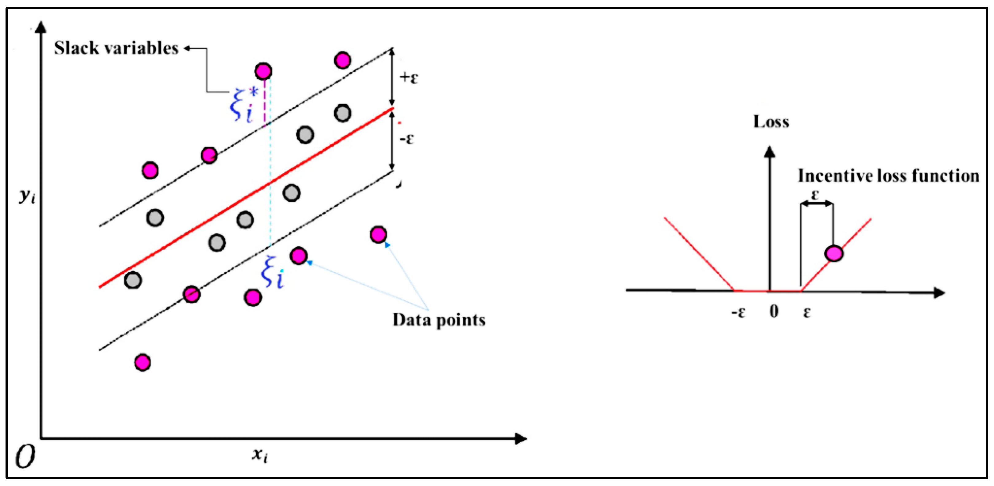
Data-driven models provide the capacity to anticipate droughts, according to Achite et al. [16]. Maca and Pech [17] utilized two types of artificial neural network (ANN) models to foresee droughts in two watersheds, namely Santa Ysabel Creek and Leaf River in South California. The results demonstrated that the hybrid ANN model outperformed the feed-forward ANN. Mokhtarzad et al. [18] employed three machine learning approaches, ANN, adaptive neuro-fuzzy inference system (ANFIS), and support vector machine (SVM), to predict meteorological drought at seasonal timescales in Iran. Although the models’ ability to predict drought was demonstrated by the results, SVM outperformed ANN and ANFIS. Similarly, Sattar et al. [19] used a Markov Bayesian classifier (MBC) to predict various classes of meteorological and hydrological drought. They reported that MBC had a range of 36% to 76% and 33% to 70% accuracy in forecasting both meteorological and hydrological drought, respectively. Jehanzaib et al. [12] compared the performance of six ML models for hydrological drought forecasting and concluded that the performance of the decision tree model was found to be superior in terms of forecast accuracy and computation time. Adnan et al. [20] integrated random vector functional link (RVFL) with the salp swarm algorithm, particle swarm optimization, hunger games search (HGS) algorithm, social spider optimization, genetic algorithm, and grey wolf optimization to forecast SPI at various timescales (3, 6, 9, and 12 months) and suggested that HGS-based RVFL can be used for drought forecasting with a high accuracy.

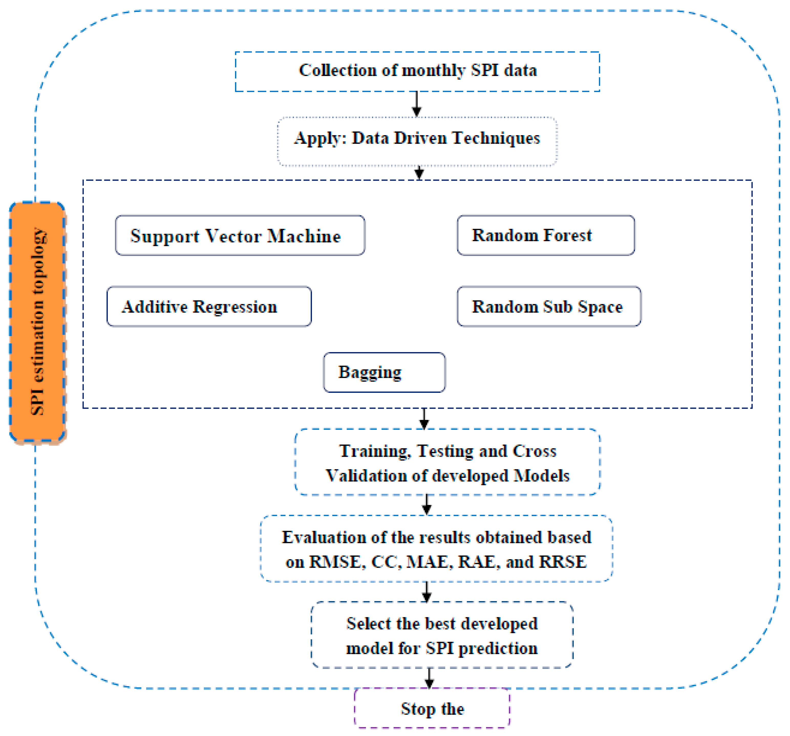
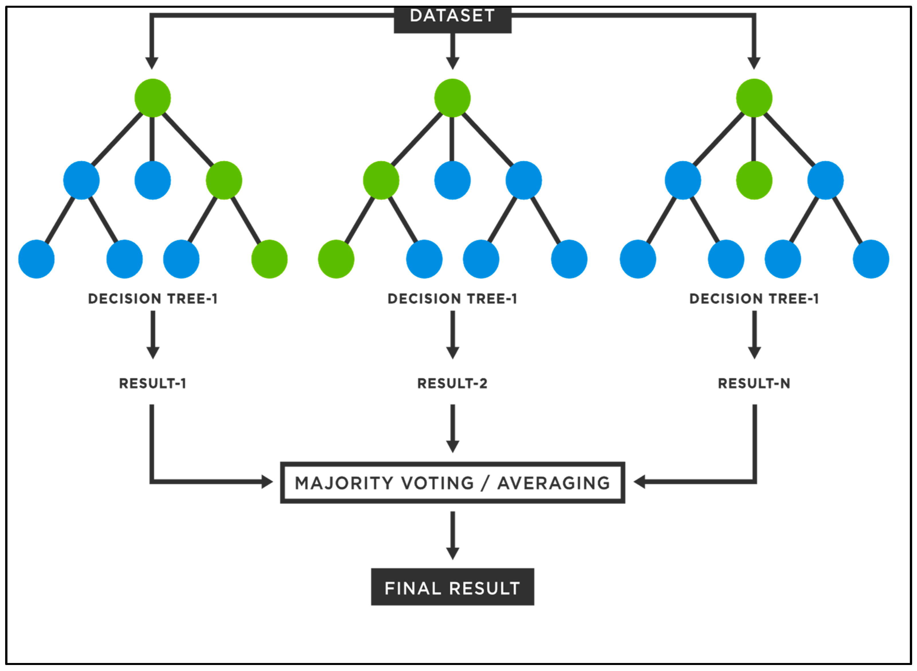
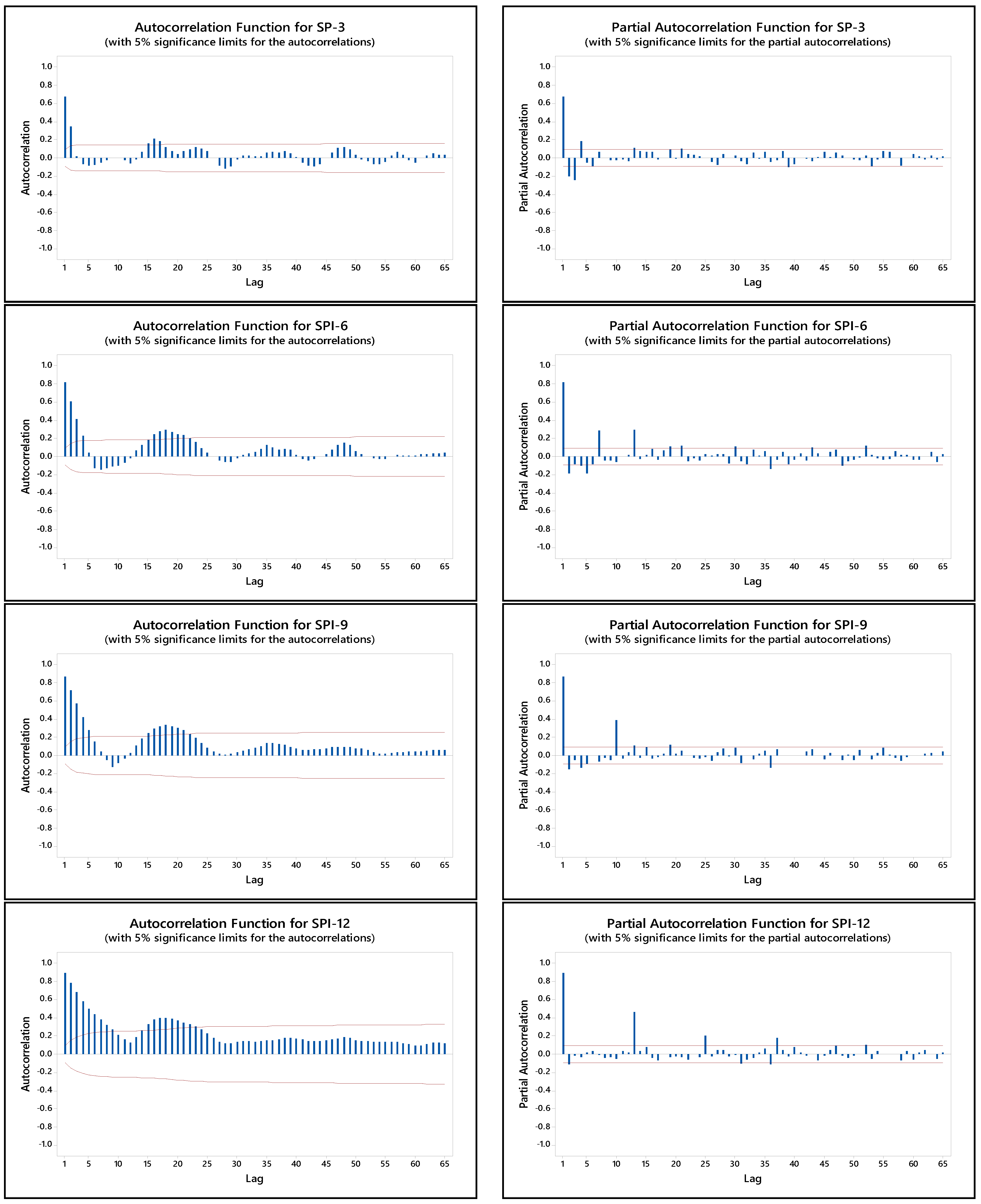
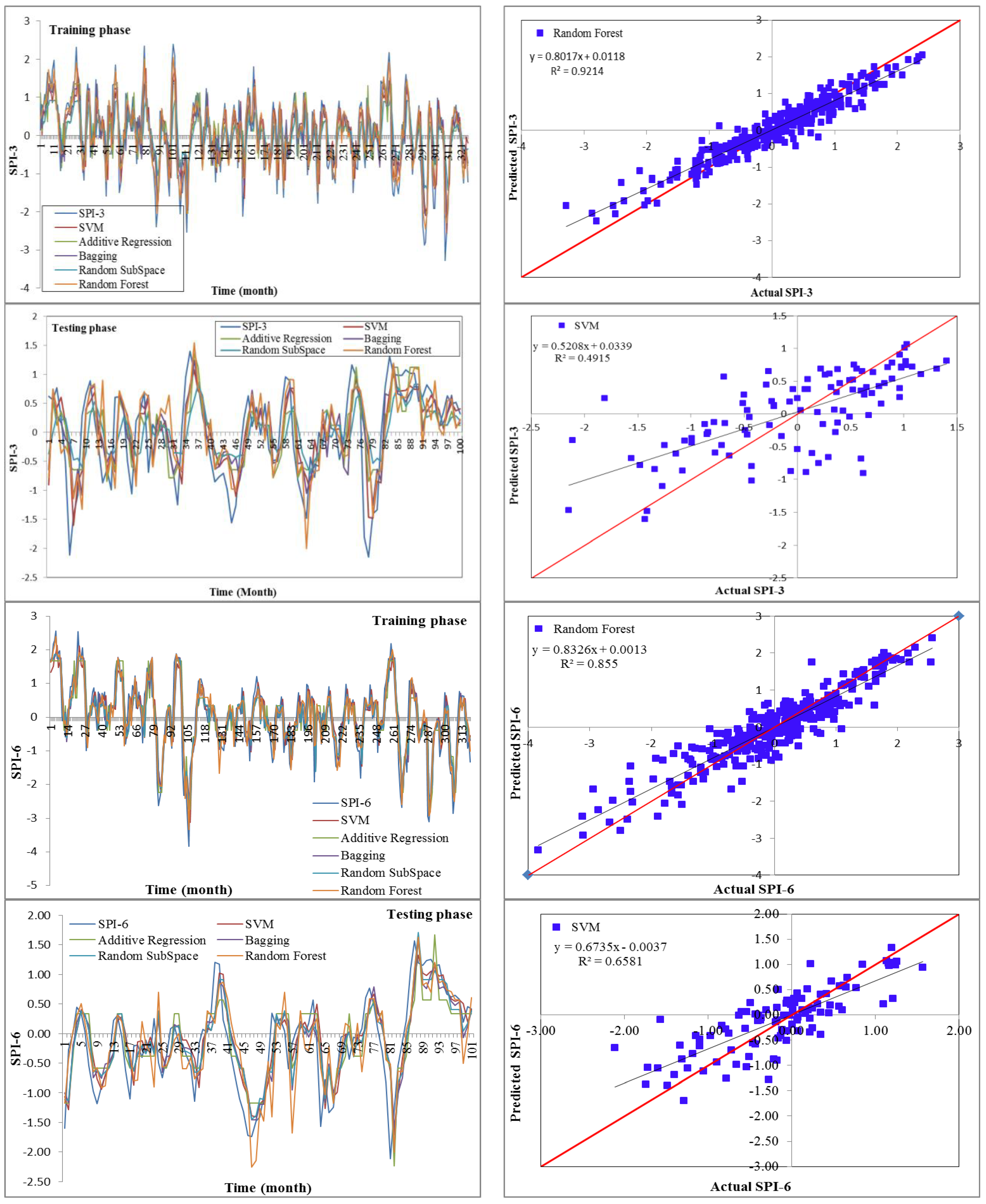
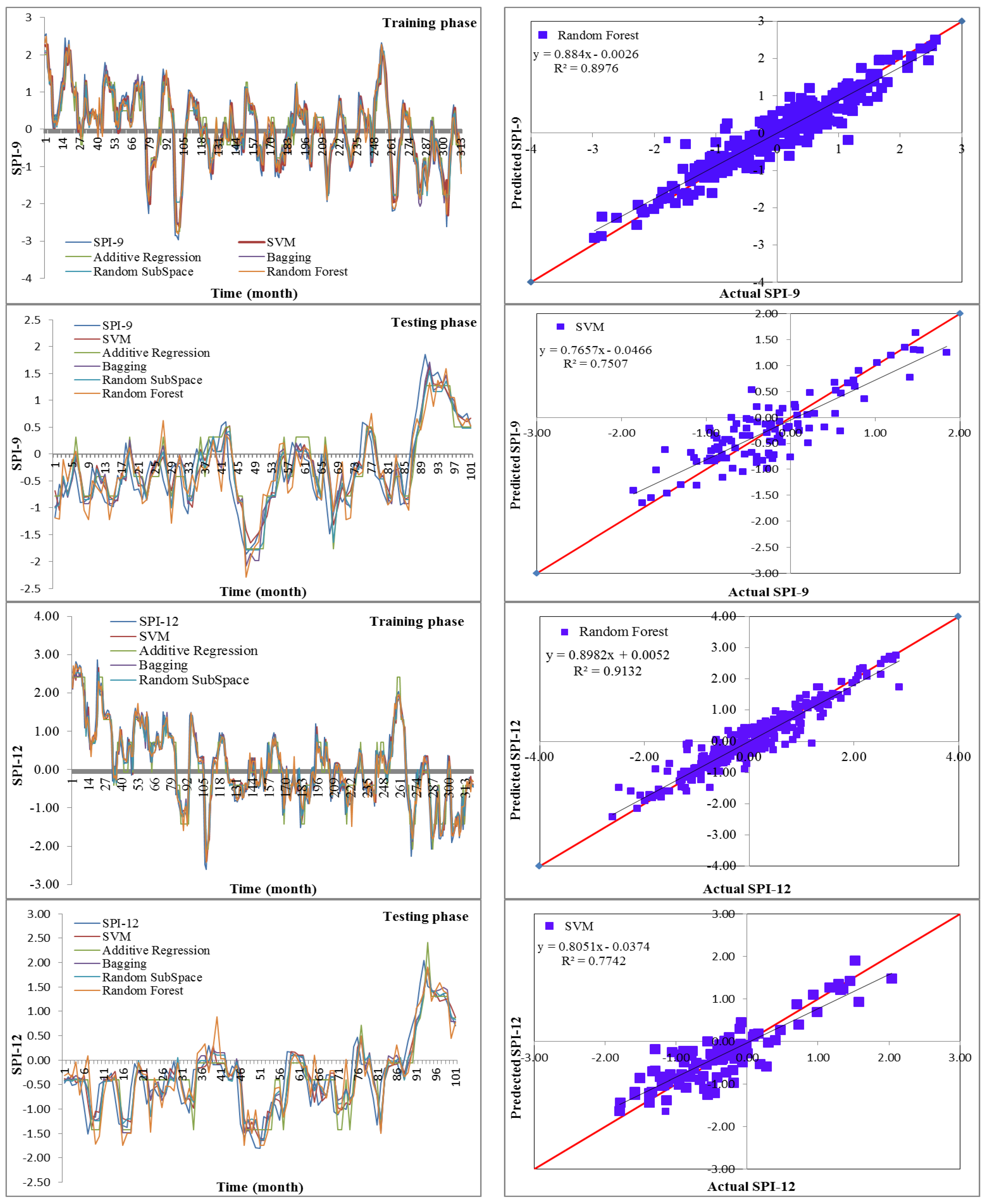
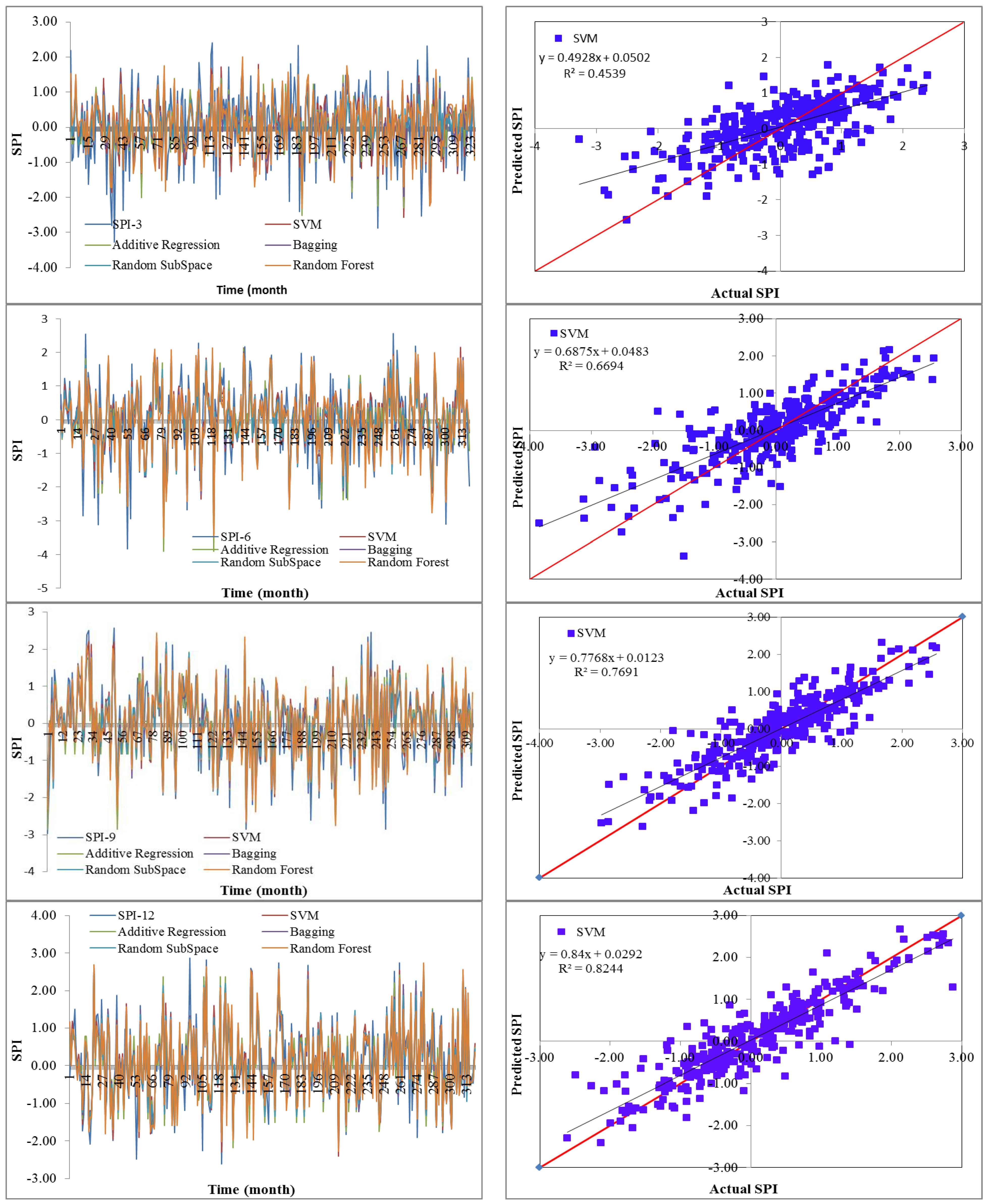
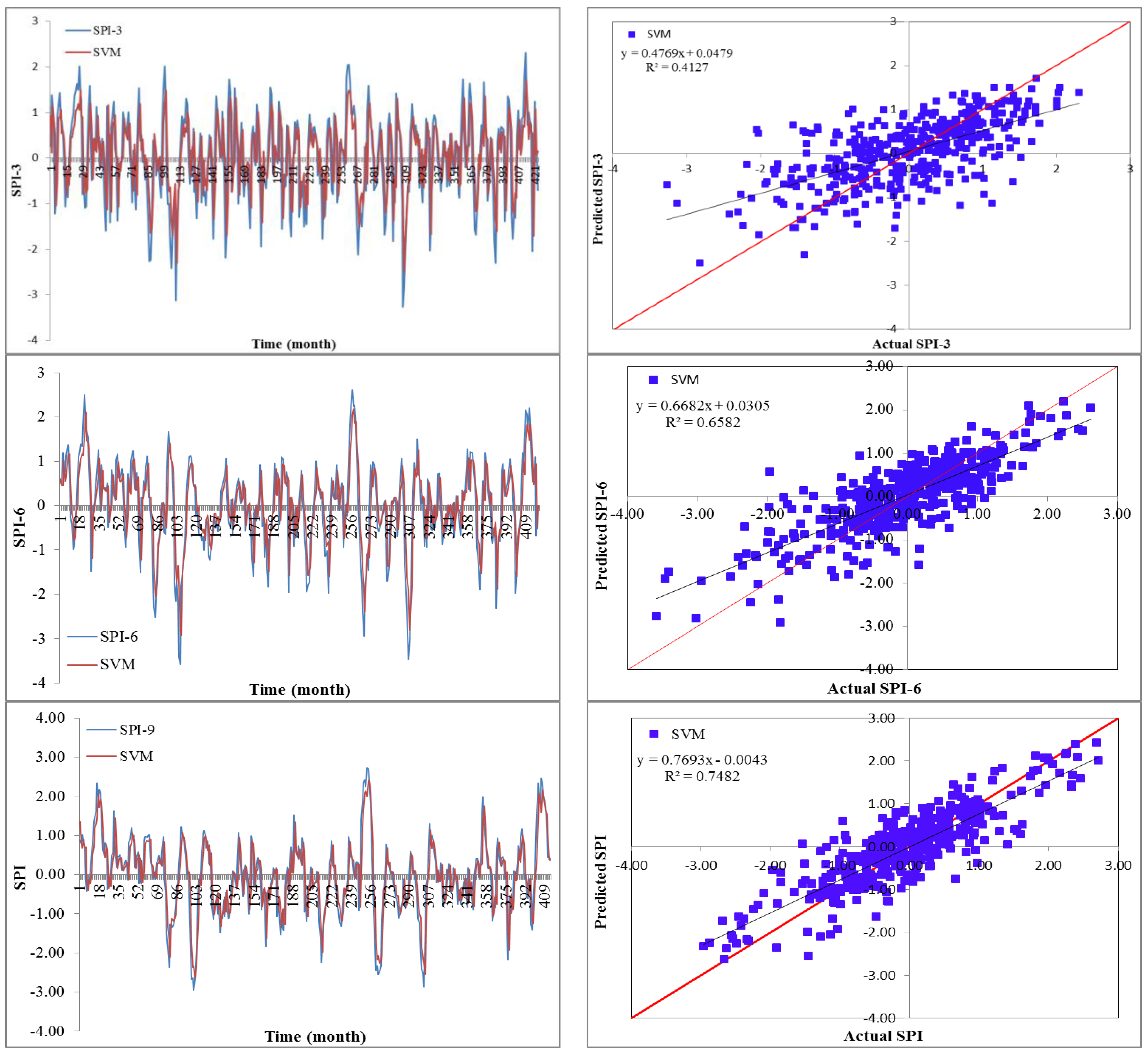
Most of the previous studies [12,13,17,18,19] utilized data-driven models for drought forecasting at a single timescale. It is critical to assess the performance of various data-driven models for drought forecasting at multiple timescales to make sound recommendations. Therefore, this study employed five state-of-the-art machine learning models, namely SVM, additive regression, bagging, random subspace, and random forest, for drought forecasting at 3-, 6-, 9-, and 12-month timescales. This study used SPI for meteorological drought estimation at various timescales due to the overwhelming benefits of the standardized drought indices. The main goals of this work were to build models for forecasting meteorological droughts using various data-driven approaches and to assess their effectiveness at various timeframes using accuracy metrics.

2. Materials and Methods

2.1. Description of the Study Area

The Wadi Mina basin in northwest Algeria served as the study region for this research. It has a total area of 4900 km² and is located between 00°22′59″ and 01°09′02″ east, as well as between 34°41′57″ and 35°35′27″ north (Figure 1). It has four significant tributaries: Wadi Haddad, Wadi Abd, Wadi Mina, and Wadi Taht. The elevation varies between 164 and 1327 m. The topography of the basin is complex and uneven. The study region features a continental climate with dramatic seasonal temperature variations, such as bitterly cold winters and sweltering summers. The yearly precipitation averages between 200 and 500 mm, with most of it falling between November and March. The average yearly temperature is between 16 and 19.5 °C. Over half of the basin is covered in a variety of plant types, including 32% scrubs, 35.8% woods, and cereal crops [21]. Monthly rainfall and runoff records are available for five rainfall and hydrometric stations over 40 years (1974–2009) (Figure 1 and

Table 1. Basic characteristics of rainfall stations.

ID		Name	Longitude	Latitude	Elevation (m)
S1	013306	Oued Abtal	0°40′33.97″ E	35°28′03.59″ N	354
S2	013401	Sidi Abdelkader Djillali	0°34′08.35″ E	35°29′20.71″ N	225

).

2.2. Standardized Precipitation Index (SPI)

SPI is calculated using the cumulative probability of the monthly precipitation measured at the observation point [22]. At a meteorological station, the parameters of a precipitation probability density function, which follow a gamma distribution, are computed over the whole observation period using Equation (1).

$$g\left(x\right)=\frac{1}{{\beta }^{\alpha }\Gamma \left(\alpha \right)}{x}^{\alpha -1}{e}^{-x/\beta }$$

(1)

where $\alpha$ and $\beta$ are the shape and scale parameters, respectively. Meanwhile, $x$ is he successive precipitation and $\Gamma \left(\alpha \right)$ is the gamma function, which is defined by Equation (2).

$$\Gamma \left(a\right)={{\displaystyle \int }}_0^{\infty }{y}^{a-1}{e}^{-y}dy$$

(2)

The alpha and beta parameters are defined as per Equation (3).

$$\alpha =\frac{1}{4A}\left(1+\sqrt{1+\frac{4A}{3}}\right), A=ln\left(\overline{x}\right)-\frac{\sum \ln \left(x_i\right)}{n}, \beta =\frac{\overline{x}}{\alpha }$$

(3)

where $n$, $\overline{x}$, and $x_i$ are the number of observations, mean precipitation, and total precipitation, respectively. The cumulative probability is estimated using Equation (4).

$$G\left(x\right)={{\displaystyle \int }}_0^{x}g\left(x\right)dx=\frac{1}{{\beta }^a\Gamma \left(a\right)}{{\displaystyle \int }}_0^x{x}^{a-1}{e}^{-x/\beta }dx$$

(4)

Equation (5) shows the cumulative probability using a mixed probability distribution to represent the likelihood of no precipitation.

$$H\left(x\right)=q+\left(1-q\right)G\left(x\right)$$

(5)

where $q$ is the likelihood of no precipitation. The SPI is calculated using Equation (6).

$$\mathrm{SPI}=\left\{\begin{array}{c}-\left(t-\frac{c_0+c_{1}t+c_2{t}^2}{1+d_{1}t+d_2{t}^2+d_3{t}^3}\right),0<H\left(x\right)\le 0.5\\ +\left(t-\frac{c_0+c_{1}t+c_2{t}^2}{1+d_{1}t+d_2{t}^2+d_3{t}^3}\right),0.5<H\left(x\right)\le 1.0\end{array}\right.$$

(6)

where $t$ is determined as shown in Equation (7).

$$t=\left\{\begin{array}{c}\sqrt{ln\left(\frac{1}{H{\left(x\right)}^2}\right)}.0<H\left(x\right)\le 0.5\\ \sqrt{ln\left(\frac{1}{{\left(1-H\left(x\right)\right)}^2}\right).}0.5<H\left(x\right)\le 1.0\end{array}\right.$$

(7)

where $c_0$, $c_1$, $c_2$, $d_1$, $d_2$, and $d_3$ are coefficients with values of:

$$c_0=2.515517 c_1=0.802853 c_2=0.010328$$

$$d_1=1.432788 d_2=0.189269 d_3=0.001308$$

Based on SPI, several classifications and the projected probability of wet and dry spells can be investigated, as shown in

Table 2. Categorization of different states of SPI.

SPI Values	Drought Category	Probability (%)
Greater than or equal to 2.0	Extremely wet	2.3
Greater than or equal to 1.5 and less than 2.0	Very wet	4.4
Greater than or equal to 1.0 and less than 1.5	Moderate wet	9.2
Greater than or equal to −1.0 and less than 1.0	Near normal	68.2
Greater than or equal to −1.0 and less than −1.5	Moderately dry	9.2
Greater than or equal to −1.5 and less than −2.0	Severely dry	4.4
Less than or equal to −2.0	Extremely dry	2.3

.

2.3. Machine Learning Models

In this study, support vector machine (SVM), additive regression (AR), bagging, random subspace (RSS), and random forest (RF) models for the estimation of SPI at 3, 6, 9, and 12 months were developed. These different models were used for anticipating drought forecasting. The flowchart of the proposed methodology for drought forecasting at the Wadi Mina basin, Algeria, is illustrated in Figure 2.

2.3.1. Support Vector Machine (SVM)

SVM establishes the decision boundary or optimal line that may categorize an n-dimensional space. The SVM algorithm searches for the extreme points that aid in the hyperplane’s creation [23]. It is a well-known approach for supervised machine learning that is utilized for both classification and regression applications [24]. Equation (8) for linear SVM can be written as follows:

$$x_1,y_1\dots \dots \dots x_n,y_n$$

(8)

where $y_1$ is either 1 or −1, depending on the linkage between the class and point $x_1$. The hyperplane that divides the group of points, $x_1$, when $y_1=1$ and $y_1=-1$. This plane is determined to optimize the distance between the hyperplane and the nearest point $x_1$ from either group. The hyperplane that satisfies Equation (9) for a set of points can be written as below:

$$w^{T}x-b=0$$

(9)

where $w$ is the hyperplane’s normal vector. The parameter, $\frac{b}{\left|\right|w\left|\right|}$ indicates how far away from the origin the hyperplane is from the normal vector. The schematic diagram and parameters of the support vector machine algorithm utilized for modeling drought forecast are shown in Figure 3.

The linear regression model is an important tool to utilize the independent variable, X, to forecast the dependent variable, Y. It is a statistical and machine learning algorithm that allows for mapping the numeric inputs to numeric outputs, fitting a best fit straight line into the datasets. The accuracy of the model is measured by least squares estimation. Equation (10) for linear regression can be written as follows:

$$Y_i={\beta }_0+{\beta }_1{X}_1+{\beta }_2{X}_2+\dots +{\beta }_p{X}_{in}+ϵ$$

(10)

where X_i and Y_i are the independent and dependent variables, respectively; ${\beta }_0$ is constant; ${\beta }_n$ is the slope coefficient of each X_i; and $ϵ$ is the model error term or residuals.

2.3.2. Additive Regression (AR)

Using the stochastic gradient boosting approach described in Friedman [25], we construct an AR model. Each iteration of AR involves drawing a random sample from the training data (without replacing it) and fitting a standalone model to the residuals from the previous iteration. In the initial fit, the training data are fitted to a standalone model without resampling, resulting in the first set of residuals, which are used to fit a stochastic gradient boosting model in the subsequent fit. The stochastic gradient boosting procedure continues until the final iteration. In Friedman [25], the predictions of all standalone models in the ensemble can be aggregated once the AR model has been trained.

Recent research has demonstrated the widespread application of Bayesian additive regression trees (BARTs) [26,27]. The BART model can define complex relations between x and y by estimating f(x) in the form y = f(x) + ε, where ε∼N (0, σ²). Furthermore, a sum of m regression trees is used, i.e., f(x) = ∑ g(x; T_j, M_j), ranging between j = 1 and j = m, which allows for the estimation of f(x). BART is expressed in Equation (11):

$$Y=f\left(\mathrm{x}\right)+\mathsf{\epsilon }={\displaystyle \sum }_{J=1}^m\mathrm{g}\left(\mathrm{x}; T_i, M_j\right)+\mathsf{\epsilon }$$

(11)

2.3.3. Bagging

A bagging method known as bootstrap aggregation (BA) was developed by Breiman [28]. In bagging, m training sets are generated, and the datasets are then fitted to m models using an easy-to-use ensemble method. As a result of averaging their outputs or voting on them, the predictions are combined. As the training dataset was modified, several classifiers were created: H_m, m = 1, …, M, which were then merged into one class. As a result, the weight of this class was derived from the combined weight of the individual predictor classes, as per Equation (12):

$$H\left(d_i\right)=sign {\displaystyle \sum }_{m=1}^M{\propto }_m+H\left(d_i\right)$$

(12)

A voting method can be used to describe the method. As α_m was determined as m = 1, …, M, then more accurate classifications would have a greater effect than less accurate classifications. As the weak Hm classification was slightly more accurate than the random classification [29], the latter was referred to as the weak H_m classification. The input datasets were also modeled using regression trees. The uniqueness of each tree was based on its ability to forecast changes in the training dataset. As a final step, the weighted average of each regression tree’s projections was calculated.

2.3.4. Random Subspace (RSS)

RSS is an ensemble machine learning algorithm that combines the prediction variables from different decision trees trained on multiple subsets of columns in the training dataset. It is a problem-independent metaheuristic technique that can be applied to a broad range of problems. Particularly when there are few training datasets compared with the amount of data, RSS is preferred [24]. It introduces randomness by selecting certain variables that are substituted at random space into the issue formulation [30]. This algorithm is a robust model assembling various weak classifiers [31,32]. It is analogous to other methods of decision trees such as bagging, which generates trees using different samples of series from the training dataset, and another method named random forest, which has ideas from bagging or the RSS model. The RSS model can easily be used with any other machine learning model, although decision trees are applied. Its performance varies notably with the choice of input variables. The original space is divided into subsets as part of the RSS algorithm’s first phase. Then, the results are attained by most polls using Equation (13):

$$\beta \left(x\right)=argma{x}_{y\in \left\{-1, 1\right\}}\sum {\delta }_{sng}\left(C^b\left(x\right)\right),y$$

(13)

where $\delta$ is the Kronecker delta symbol,$C^b\left(x\right)$ is the classification integration ($C=1, 2,\dots )$, and $y\in \left\{-1, 1\right\}$ is a class label of the classifier. The graphic schematic diagram of the RSS algorithm for drought forecasting modeling is shown in Figure 4.

2.3.5. Random Forest (RF)

Breiman [33] proposed the RF algorithm, where the explanatory variables may be either continuous or categorical. The model has been used effectively for both regression and classification problems. It constructs several decision trees. The complexity of the non-linear relationship between the explanatory and target variables can easily be reduced instead of a detailed numerical representation because it causes more complexity in the model. The model is formed by selecting the input features randomly at each node. The regression in the model has a similar structure to the classification tree. The output is obtained by averaging each tree’s output (Figure 5). The model is efficient with internally multiple classes, robustness to the outliers in the model, accuracy in prediction, self-tuning ability, and deals with the large or small sample of the datasets to the other machine learning models.

The adaptive bagging algorithm was developed to reduce bias and improve the model’s classification and regression efficiency. Out-of-bag (OOB) estimates error, strength, and model correlation with a selection of random features. Generally, the out-of-bag estimates in the model consider the combination of one-third of classifiers. The error rate is reduced due to an increment in an assortment of classifiers in classification through the RF model. Bootstrap is a statistical resample approach used to evaluate the statistical parameters of the sample selected randomly. It is observed from the available dataset that some observations not considered in the sample, known as out-of-bag data, are used to evaluate the generalization error and elaborate on the importance of the variables. The rate of generalization error in regression is defined as per Equation (14):

$${\mathrm{MSE}}_{\mathrm{oob}}=\frac{1}{N}{\displaystyle \sum }_{i=1}^N{y}_i-f_{\mathrm{oob}}\left(x_i\right)²$$

(14)

where $f_{\mathrm{oob}}\left(x_i\right)$ = OOB is the prediction for ith observations. For the classification, the rate of generalization error helps to estimate the class-wise rate of error for each class in the model, which can be evaluated using the rate of OOB error, as per Equation (15):

$${\mathrm{E}}_{\mathrm{oob}}=\frac{1}{N}{\displaystyle \sum }_{i=1}^N{y}_i\ne f_{\mathrm{oob}}\left(x_i\right)$$

(15)

3. Model Evaluation

To assess the performance of the ML algorithm, a comparison between the estimated/modeled values using ML methods and the observed values of the SPI was made at various timescales. Five performance metrics indices including correlation coefficient (CC), mean absolute error (MAE), root mean square error (RMSE), relative absolute error (RAE), and root relative squared error (RRSE) were used to quantitatively validate the models. The various metrics are calculated as depicted in

Table 3. Descriptions of indices for data mining techniques supported by mathematical formulations.

Performance Indices	Formula	Range	Ideal Level	Description
Correlation coefficient	$\mathrm{CC}=\frac{{\sum }_{i=1}^N\left[\left({\mathrm{SPI}}_{Obs}-\overline{{\mathrm{SPI}}_{Obs}}\right)\left({\mathrm{SPI}}_{Pre}-\overline{{\mathrm{SPI}}_{Pre}}\right)\right]}{\sqrt{{\sum }_{i=1}^N{\left({\mathrm{SPI}}_{Obs}-\overline{{\mathrm{SPI}}_{Obs}}\right)}^2}\sqrt{{\sum }_{i=1}^N{\left({\mathrm{SPI}}_{Pre}-\overline{{\mathrm{SPI}}_{Pre}}\right)}^2}}$	(−1 to +1)	+1	Calculates how similar the observed value is to the expected value.
Mean absolute error	$\mathrm{MAE}=\frac{1}{N}{\displaystyle \sum _{i=1}^N}\left|{\mathrm{SPI}}_{Pre},-{\mathrm{SPI}}_{Obs}\right|$	(0 to ∞)	0	Analyzes the error size on an average.
Root mean square error	$\mathrm{RMSE}=\sqrt{\frac{1}{N}{\displaystyle \sum _{i=1}^N}{\left[{\mathrm{SPI}}_{Pre}-{\mathrm{SPI}}_{Obs}\right]}^2}$	(0 to ∞)	0	Indicates how observed values differ from estimated values.
Relative absolute error	$\mathrm{RAE}={\displaystyle \sum _{i=1}^N}\left|{\mathrm{SPI}}_{Pre}-{\mathrm{SPI}}_{Obs}\right|/{\displaystyle \sum _{i=1}^N}\left|\overline{{\mathrm{SPI}}_{Obs}}-{\mathrm{SPI}}_{Obs}\right|$	(0 to ∞)	0	Conducts a performance evaluation of the machine learning algorithm.
Root relative squared error	$\mathrm{RRSE}={\displaystyle \sum _{i=1}^N}{\left({\mathrm{SPI}}_{Pre}-{\mathrm{SPI}}_{Obs}\right)}^2/{\displaystyle \sum _{i=1}^N}{\left(\overline{{\mathrm{SPI}}_{Obs}}-{\mathrm{SPI}}_{Obs}\right)}^2$	(0 to ∞)	0	In contrast to RMSE, the relative squared error (RSE) allows the comparison of models with errors expressed in various units.

.

Where; ${\mathrm{SPI}}_{Pre}-{\mathrm{SPI}}_{Obs}$ are ith predicted and observed SPI values, respectively, and $\overline{{\mathrm{SPI}}_{Pre}}$ and $\overline{{\mathrm{SPI}}_{Obs}}$ are predicted and observed average values of SPI, respectively. Besides, N represents the number of data sets.

4. Results and Discussion

4.1. Input Variables Selection

The meteorological drought index (SPI) was calculated across a range of timeframes (3–12 months). As shown in Figure 6, PACF was applied to determine the optimum lags of the SPI index [34]. The lag values that provide this 95% confidence bound were selected as the inputs. For all timescales, t-1 lag formed the largest correlation [16]. The SPI index provided a remarkably large correlation of t-10 lag for the 9-month timescale.

Table 4. Input−output relationships for SPI prediction.

Sub Basin Name	Inputs Variables	Target Variable
Sub-basin 1	SPI-3 (t-1); SPI-3 (t-2)	SPI-3
	SPI-6 (t-1); SPI-6 (t-2); SPI-6 (t-5); SPI-6 (t-7)	SPI-6
	SPI-9 (t-1)	SPI-9
	SPI-12 (t-1)	SPI-12

displayed the optimal input combination for SPI prediction used in this study. To examine the temporal gaps between the current and previous indices, the statistical approach attempted to extract lagging information from the signal. After that, the optimal inputs for each time lag were found by conducting statistical analysis on the lagged combination coefficients and by analyzing the correlations between them.

4.2. Comparison Models of SPI Drought Index

The SPI drought index is predicted in five sub-basins using five machine learning models: SVM, AR, B, RSS, and RF. For the training and testing stages,

Table 5. Evaluation metrics of the model outputs for various timelines during the training and testing phases.

Model	Training Phase					Testing Phase
	CC	MAE	RMSE	RAE	RRSE	CC	MAE	RMSE	RAE	RRSE
SPI-3
Support vector machine	0.684	0.557	0.725	70.225	73.247	0.701	0.453	0.579	68.038	71.463
Additive regression	0.711	0.544	0.696	68.638	70.366	0.677	0.475	0.596	71.313	73.552
Bagging	0.796	0.466	0.606	58.722	61.195	0.645	0.478	0.622	71.721	76.792
Random subspace	0.667	0.608	0.765	76.724	77.278	0.542	0.553	0.684	83.019	84.405
Random forest	0.960	0.230	0.304	29.056	30.683	0.592	0.526	0.682	78.926	84.088
SPI-6
Support vector machine	0.824	0.447	0.596	56.157	56.729	0.811	0.355	0.452	58.505	57.447
Additive regression	0.833	0.442	0.581	55.454	55.309	0.770	0.402	0.492	66.219	62.530
Bagging	0.864	0.399	0.529	50.116	50.396	0.800	0.360	0.461	59.361	58.638
Random subspace	0.864	0.403	0.530	50.560	50.434	0.811	0.359	0.450	59.243	57.137
Random forest	0.925	0.303	0.401	38.083	38.161	0.735	0.420	0.545	69.188	69.239
SPI-9
Support vector machine	0.882	0.359	0.472	46.288	47.242	0.866	0.306	0.381	45.599	46.795
Additive regression	0.878	0.371	0.479	47.823	47.953	0.822	0.362	0.440	53.940	53.993
Bagging	0.909	0.321	0.415	41.398	41.605	0.845	0.339	0.414	50.576	50.830
Random subspace	0.897	0.336	0.441	43.272	44.152	0.863	0.315	0.388	46.932	47.606
Random forest	0.947	0.233	0.320	30.030	32.041	0.806	0.357	0.463	53.275	56.859
SPI-12
Support vector machine	0.908	0.305	0.431	37.412	41.963	0.880	0.283	0.371	38.061	41.520
Additive regression	0.898	0.341	0.454	41.772	44.268	0.823	0.343	0.453	46.134	50.702
Bagging	0.927	0.278	0.386	34.138	37.596	0.866	0.305	0.394	41.092	44.043
Random subspace	0.924	0.283	0.394	34.728	38.386	0.874	0.297	0.380	39.914	42.553
Random forest	0.956	0.212	0.303	25.977	29.514	0.808	0.381	0.483	51.226	54.028

displays the model outcomes across all timelines. Training (70%) and testing (30%) are the two phases into which the data was split. The results indicate that SPI-12 performed the best when compared with the other timeframes. Moreover, RF (CC = 0.960, MAE = 0.230, RMSE = 0.304, RAE = 29.056, and RRSE = 30.683) exhibited the best performance for SPI-3 compared with the other models for the training phase. According to CC, MAE, RMSE, RAE, and RRSE with SPI-12 during the testing phase, SVM was able to achieve 0.880, 0.283, 0.371, 38.061, and 41.520, respectively.

Figure 7 illustrates the scatterplot of the observed and predicted SPI for the training and testing phases. The results showed that the SPI for the proposed SVM model closely matched the observed values during the testing phase. Extreme wetness and drought values were seen to be more properly approximated using SVM.

Cross-validation is a statistical method that splits data into two segments: one for learning or training a model and the other for verifying the model. It was used in this study to analyze and compare machine learning algorithms. It is a resampling process used to assess machine learning models and determine how well the model would perform on an independent test dataset. In this study, four folds were used for all of the algorithms developed in order to cross-validate all of the datasets, as shown in Figure 8. All of the datasets were divided into four parts to evaluate the performance of models in terms of accuracy and statistical errors.

Table 6. Cross-validation for the ML models for estimating SPI at 3, 6, 9, and 12 months.

Model	CC	MAE	RMSE	RAE	RRSE
SPI-3
Support vector machine	0.674	0.569	0.734	71.44	73.94
Additive regression	0.645	0.600	0.758	75.3839	76.384
Bagging	0.638	0.600	0.764	75.325	76.964
Random subspace	0.586	0.642	0.811	80.603	81.653
Random forest	0.615	0.611	0.797	76.788	80.255
SPI-6
Support vector machine	0.818	0.455	0.606	56.654	57.369
Additive regression	0.765	0.518	0.683	64.604	64.637
Bagging	0.799	0.481	0.634	59.940	60.016
Random subspace	0.799	0.481	0.632	59.915	59.885
Random forest	0.749	0.565	0.724	70.457	68.512
SPI-9
Support vector machine	0.877	0.368	0.480	46.883	47.479
Additive regression	0.840	0.420	0.543	53.613	53.726
Bagging	0.856	0.396	0.517	50.529	51.186
Random subspace	0.856	0.395	0.517	50.355	51.152
Random forest	0.839	0.434	0.555	55.339	54.907
SPI-12
Support vector machine	0.908	0.305	0.431	37.412	41.963
Additive regression	0.898	0.341	0.454	41.772	44.268
Bagging	0.927	0.278	0.386	34.138	37.596
Random subspace	0.924	0.283	0.394	34.728	38.386
Random forest	0.956	0.212	0.303	25.977	29.514

demonstrated that the SVM model outperformed other models in terms of performance. The correlation coefficients ranged from 0.67 to 0.91 under all of the SPI periods, except for SPI 12. RF was the best model for predicting SPI-12. At the same time, statistical errors were the lowest values compared with other algorithms (Table 6). In addition, time series and scatter plots are presented in Figure 9 to show the performance of the developed models.

As illustrated in

Table 7. Performance validation of SVM at sub-basin 2.

	CC	MAE	RMSE	RAE	RRSE
SPI-3	0.642	0.575	0.751	72.927	77.370
SPI-6	0.811	0.445	0.580	58.958	58.548
SPI-9	0.865	0.379	0.493	51.304	50.172
SPI-12	0.885	0.331	0.466	42.81	46.639

, at sub-basin 2, the SVM model also gave higher outcomes for correlation coefficients (CC) and statistical errors, such as MAE, RMSE, RAE, and RRSE, than other data-driven models. The CC values varied from 0.642 to 885 for the SPI periods from 3 to 12 months. The time series and scatter plots for the SVM model were created to show its accuracy in SPI modeling under different months for the second basin (Figure 10). This study concludes and recommends using SVM for the studied stations for modeling the drought SPI index for better water resources management, monitoring, and planning.

This model was validated by comparing its performance across the results reported in the literature. The SVM model (CC = 0.674, MAE = 0.569, RMSE = 0.734, RAE = 71.44, and RRSE = 73.94) outperformed the ANFIS model trained using the nomadic people optimization algorithm (NPA) (RMSE = 2.21, MAE = 2.15, NSE = 0.91, PBIAS = 0.15, and R2 = 0.92) to forecast the 3-month SPI. The ANFIS-NPA model was reported to be the best-performing model compared with the ANFIS, RBFNN, MLP, and SVM models optimized using the krill algorithm, salp swarm algorithm, and bat algorithm, along with the standalone models [35]. This affirms the robustness and outperformance of the developed models compared with those found in the previous studies.

5. Conclusions and Recommendations

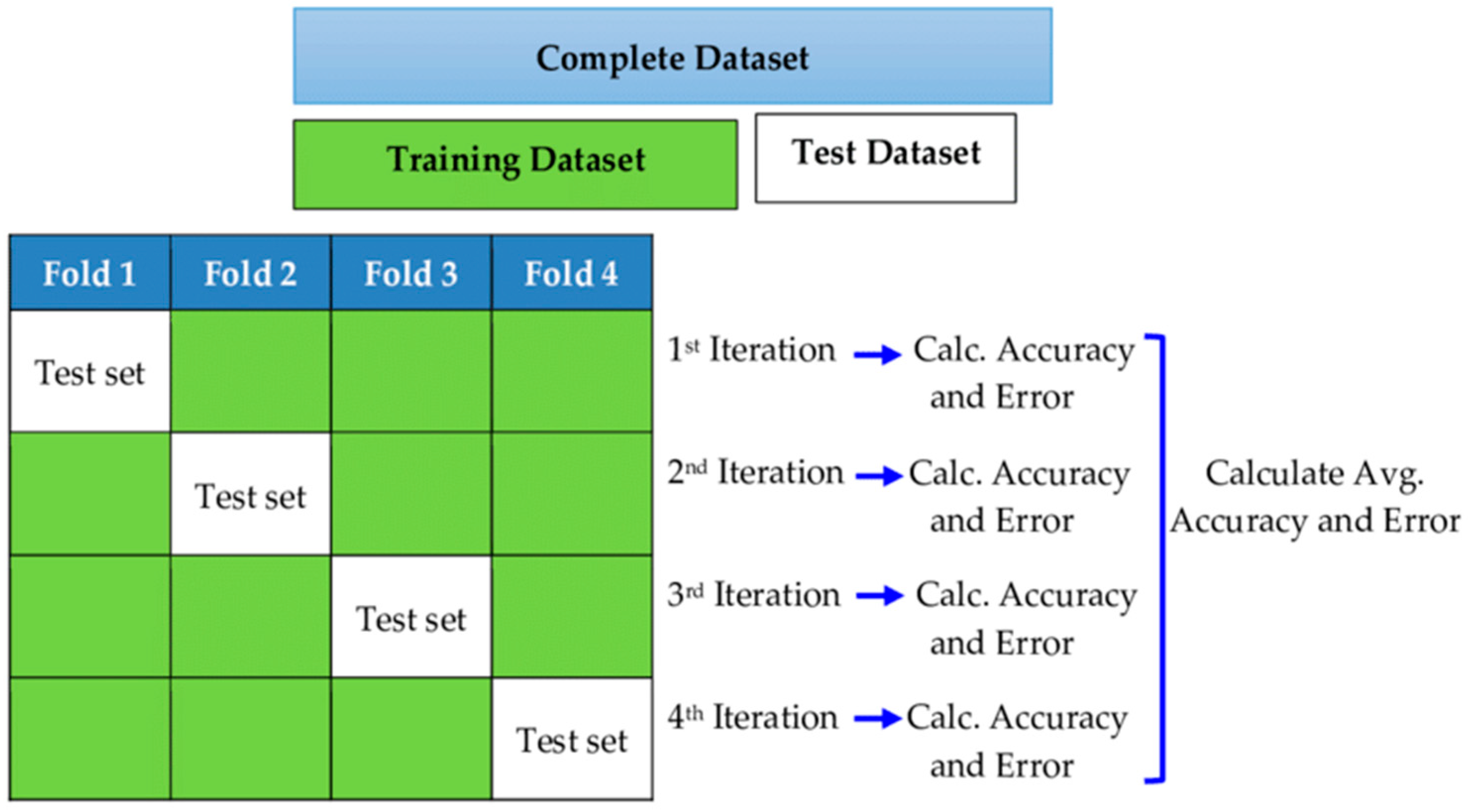
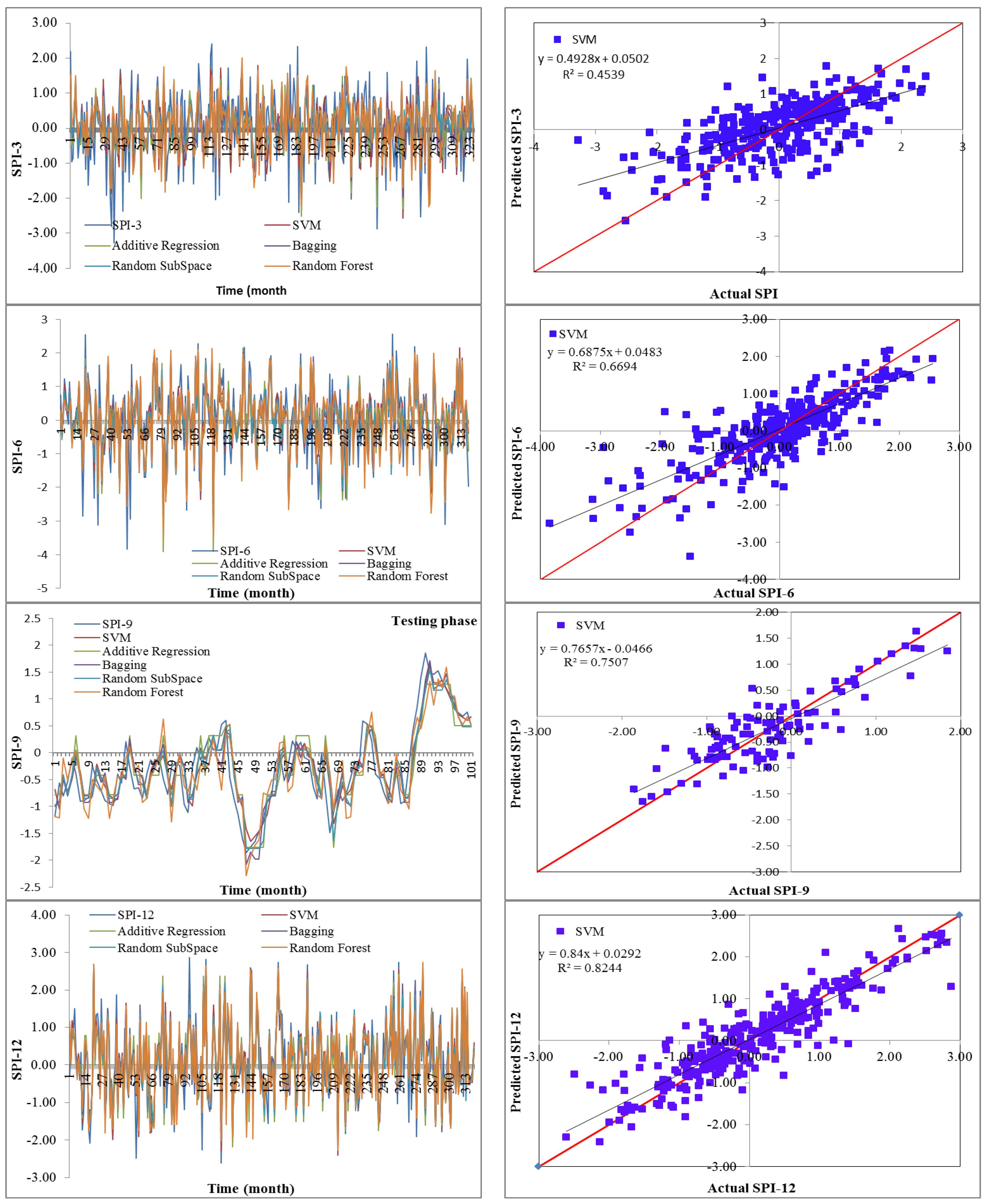
Drought has a detrimental influence on agricultural output, land and soil quality, desertification, food security, and water resources. Despite this, because of its complexity and several factors at various temporal and geographic dimensions, drought continues to be among the least understood natural phenomena. In the last ten years, the use of machine learning approaches to develop trustworthy models with high computational capabilities has drawn attention to the field of drought modelling. In this context, this research applied five machine learning models, namely support vector machine, additive regression, bagging, random subspace, and random forest, to anticipate a meteorological drought in the Wadi Mina basin, Algeria. Five performance assessment metrics were used to compare the performance of the developed models. The results indicated that SPI-12 performed the best when compared with the other timeframes. According to CC, MAE, RMSE, RAE, and RRSE with SPI-12 during the testing phase, SVM was able to achieve 0.880, 0.283, 0.371, 38.061, and 41.520, respectively. The results from cross-validation demonstrated that the SVM model outperformed the other models. The correlation coefficients ranged from 0.674 to 0.908 under all of the SPI periods. Its performance was validated at sub-basin 2 and satisfactory results were achieved. The suggested model provided a practical tool for managing intricate drought dynamics at various periods. Future studies should investigate the application of the proposed model in other basins of different countries. A trustworthy intelligent system might be developed using the suggested model to anticipate meteorological drought across a variety of timescales, aid in the management of sustainable water resources, and identify corrective actions in stations.

References

1. Dai, A. Increasing drought under global warming in observations and models. Nat. Clim. Chang. 2013, 3, 52–58. [Google Scholar] [CrossRef]
2. Kim, T.W.; Jehanzaib, M. Drought risk analysis, forecasting and assessment under climate change. Water 2020, 12, 1862. [Google Scholar] [CrossRef]
3. Zhao, L.; Lyu, A.; Wu, J.; Hayes, M.; Tang, Z.; He, B.; Liu, J.; Liu, M. Impact of meteorological drought on streamflow drought in Jinghe River Basin of China. Chin. Geogr. Sci. 2014, 24, 694–705. [Google Scholar] [CrossRef]
4. Crutchfield, S. USDA Economic Research Service-US Drought 2012: Farm and Food Impacts. 2012. Available online: https://drought.unl.edu/archive/assessments/USDA-ERS-2012-farm-food-impacts.pdf (accessed on 8 December 2022).
5. Mishra, A.K.; Singh, V.P. Drought modelling—A review. J. Hydrol. 2011, 403, 157–175. [Google Scholar] [CrossRef]
6. Cancelliere, A.; Mauro, G.D.; Bonaccorso, B.; Rossi, G. Drought forecasting using the standardized precipitation index. Water Resour. Manag. 2007, 21, 801–819. [Google Scholar] [CrossRef]
7. Heim, R.R., Jr. A review of twentieth-century drought indices used in the United States. Bull. Am. Meteorol. Soc. 2002, 83, 1149–1166. [Google Scholar] [CrossRef]
8. Jehanzaib, M.; Shah, S.A.; Kim, J.E.; Kim, T.W. Exploring spatio-temporal variation of drought characteristics and propagation under climate change using multi-model ensemble projections. Nat. Hazards 2022, 1–21. [Google Scholar] [CrossRef]
9. Jehanzaib, M.; Sattar, M.N.; Lee, J.H.; Kim, T.W. Investigating effect of climate change on drought propagation from meteorological to hydrological drought using multi-model ensemble projections. Stoch. Environ. Res. Risk Assess. 2020, 34, 7–21. [Google Scholar] [CrossRef]
10. Zhao, J.; Xu, J.; Xie, X.; Lu, H. Drought monitoring based on TIGGE and distributed hydrological model in Huaihe River Basin, China. Sci. Total Environ. 2016, 553, 358–365. [Google Scholar] [CrossRef]
11. Durbach, I.; Merven, B.; McCall, B. Expert elicitation of autocorrelated time series with application to e3 (energy-environment-economic) forecasting models. Environ. Model. Softw. 2017, 88, 93–105. [Google Scholar] [CrossRef]
12. Jehanzaib, M.; Bilal Idrees, M.; Kim, D.; Kim, T.W. Comprehensive evaluation of machine learning techniques for hydrological drought forecasting. J. Irrig. Drain. Eng. 2021, 147, 04021022. [Google Scholar] [CrossRef]
13. Anshuka, A.; van Ogtrop, F.F.; Willem Vervoort, R. Drought forecasting through statistical models using standardised precipitation index: A systematic review and meta-regression analysis. Nat. Hazards 2019, 97, 955–977. [Google Scholar] [CrossRef]
14. Solomatine, D.P.; Ostfeld, A. Data-driven modelling: Some past experiences and new approaches. J. Hydroinformatics 2008, 10, 3–22. [Google Scholar] [CrossRef]
15. Abrahart, R.J.; See, L.M.; Solomatine, D.P. (Eds.) Practical Hydroinformatics: Computational Intelligence and Technological Developments in Water Applications; Springer Science & Business Media: Berlin, Germany, 2008; Volume 68. [Google Scholar]
16. Achite, M.; Jehanzaib, M.; Elshaboury, N.; Kim, T.W. Evaluation of machine learning techniques for hydrological drought modeling: A case study of the Wadi Ouahrane basin in Algeria. Water 2022, 14, 431. [Google Scholar] [CrossRef]
17. Maca, P.; Pech, P. Forecasting SPEI and SPI drought indices using the integrated artificial neural networks. Comput. Intell. Neurosci. 2016, 2016, 14. [Google Scholar] [CrossRef]
18. Mokhtarzad, M.; Eskandari, F.; Jamshidi Vanjani, N.; Arabasadi, A. Drought forecasting by ANN, ANFIS, and SVM and comparison of the models. Environ. Earth Sci. 2017, 76, 729. [Google Scholar] [CrossRef]
19. Sattar, M.N.; Jehanzaib, M.; Kim, J.E.; Kwon, H.H.; Kim, T.W. Application of the hidden Markov bayesian classifier and propagation concept for probabilistic assessment of meteorological and hydrological droughts in South Korea. Atmosphere 2020, 11, 1000. [Google Scholar] [CrossRef]
20. Adnan, R.M.; Mostafa, R.R.; Islam, A.R.M.T.; Gorgij, A.D.; Kuriqi, A.; Kisi, O. Improving drought modeling using hybrid random vector functional link methods. Water 2021, 13, 3379. [Google Scholar] [CrossRef]
21. Achite, M.; Ouillon, S. Suspended sediment transport in a semiarid watershed, Wadi Abd, Algeria (1973–1995). J. Hydrol. 2007, 343, 187–202. [Google Scholar] [CrossRef]
22. Awange, J.L.; Mpelasoka, F.; Goncalves, R.M. When every drop counts: Analysis of droughts in Brazil for the 1901-2013 period. Sci. Total Environ. 2016, 566, 1472–1488. [Google Scholar] [CrossRef]
23. Sain, S.R. The nature of statistical learning theory. Technometrics 1996, 38, 409. [Google Scholar] [CrossRef]
24. Kushwaha, N.L.; Rajput, J.; Elbeltagi, A.; Elnaggar, A.Y.; Sena, D.R.; Vishwakarma, D.K.; Mani, I.; Hussein, E.E. Data intelligence model and meta-heuristic algorithms-based pan evaporation modelling in two different agro-climatic zones: A case study from Northern India. Atmosphere 2021, 12, 1654. [Google Scholar] [CrossRef]
25. Friedman, J.H. Stochastic gradient boosting. Comput. Stat. Data Anal. 2002, 38, 367–378. [Google Scholar] [CrossRef]
26. Tan, Y.V.; Roy, J. Bayesian additive regression trees and the General BART model. Stat. Med. 2019, 38, 5048–5069. [Google Scholar] [CrossRef] [PubMed]
27. Sparapani, R.; Logan, B.; Laud, P. MCW Biostatistics Technical Report 72 Nonparametric Failure Time: Time-to-event Machine Learning with Heteroskedastic Bayesian Additive Regression Trees and Low Information Omnibus Dirichlet Process Mixtures. 2021. Available online: https://www.mcw.edu/-/media/MCW/Departments/Biostatistics/tr72.pdf?la=en (accessed on 8 December 2022).
28. Breiman, L. Bagging predictors. Mach. Learn. 1996, 24, 123–140. [Google Scholar] [CrossRef]
29. Breiman, L. Arcing the Edge; Technical Report 486; Statistics Department, University of California at Berkeley: Berkeley, CA, USA, 1997. [Google Scholar]
30. Vishwakarma, D.K.; Ali, R.; Bhat, S.A.; Elbeltagi, A.; Kushwaha, N.L.; Kumar, R.; Rajput, J.; Heddam, S.; Kuriqi, A. Pre-and post-dam river water temperature alteration prediction using advanced machine learning models. Environ. Sci. Pollut. Res. 2022, 29, 83321–83346. [Google Scholar] [CrossRef]
31. Al-rimy, B.A.S.; Maarof, M.A.; Shaid, S.Z.M. Crypto-ransomware early detection model using novel incremental bagging with enhanced semi-random subspace selection. Future Gener. Comput. Syst. 2019, 101, 476–491. [Google Scholar] [CrossRef]
32. Plumpton, C.O.; Kuncheva, L.I.; Oosterhof, N.N.; Johnston, S.J. Naive random subspace ensemble with linear classifiers for real-time classification of fMRI data. Pattern Recognit. 2012, 45, 2101–2108. [Google Scholar] [CrossRef]
33. Breiman, L. Random forests. Mach. Learn. 2001, 45, 5–32. [Google Scholar] [CrossRef]
34. Deo, R.C.; Tiwari, M.K.; Adamowski, J.F.; Quilty, J.M. Forecasting effective drought index using a wavelet extreme learning machine (W-ELM) model. Stoch. Environ. Res. Risk Assess. 2017, 31, 1211–1240. [Google Scholar] [CrossRef]
35. Mohamadi, S.; Sammen, S.S.; Panahi, F.; Ehteram, M.; Kisi, O.; Mosavi, A.; Ahmed, A.N.; El-Shafie, A.; Al-Ansari, N. Zoning map for drought prediction using integrated machine learning models with a nomadic people optimization algorithm. Nat. Hazards 2020, 104, 537–579. [Google Scholar] [CrossRef]
Figure 1. Study area, as well as pluviometric and hydrometric network.
Water 15 00765 g001
Figure 2. Flowchart of the proposed methodology.
Water 15 00765 g002
Figure 3. Graphic schematic layout of the support vector machine.
Water 15 00765 g003
Figure 4. The block diagram of the random subspace.
Water 15 00765 g004
Figure 5. Illustration of random forest trees.
Water 15 00765 g005
Figure 6. Autocorrelation and partial autocorrelation function for SPI across different timeframes.
Water 15 00765 g006
Figure 7. Plots showing predicted and observed SPI values for 3, 6, 9, and 12 timeframes during training and testing periods at sub-basin 1.
Water 15 00765 g007aWater 15 00765 g007b
Figure 8. Cross-validation layout for evaluation of the ML algorithms based on 4 k folds.
Water 15 00765 g008
Figure 9. Plots showing the predicted and observed SPI values for 3-, 6-, 9-, and 12-month timeframes during the cross-validation periods at sub-basin 1.
Water 15 00765 g009aWater 15 00765 g009b
Figure 10. Plots showing the predicted and observed SPI values for 3, 6, 9, and 12 month timeframes during validating the performance at sub-basin 2.
Water 15 00765 g010aWater 15 00765 g010b