
Environmental Stable and Radioactive Isotopes in the Assessment of Thermomineral Waters in Lisbon Region (Portugal): Contributions for a Conceptual Model

Abstract
:1. Introduction
2. Climatology, Geological and Hydrogeological Setting
2.1. Climatology
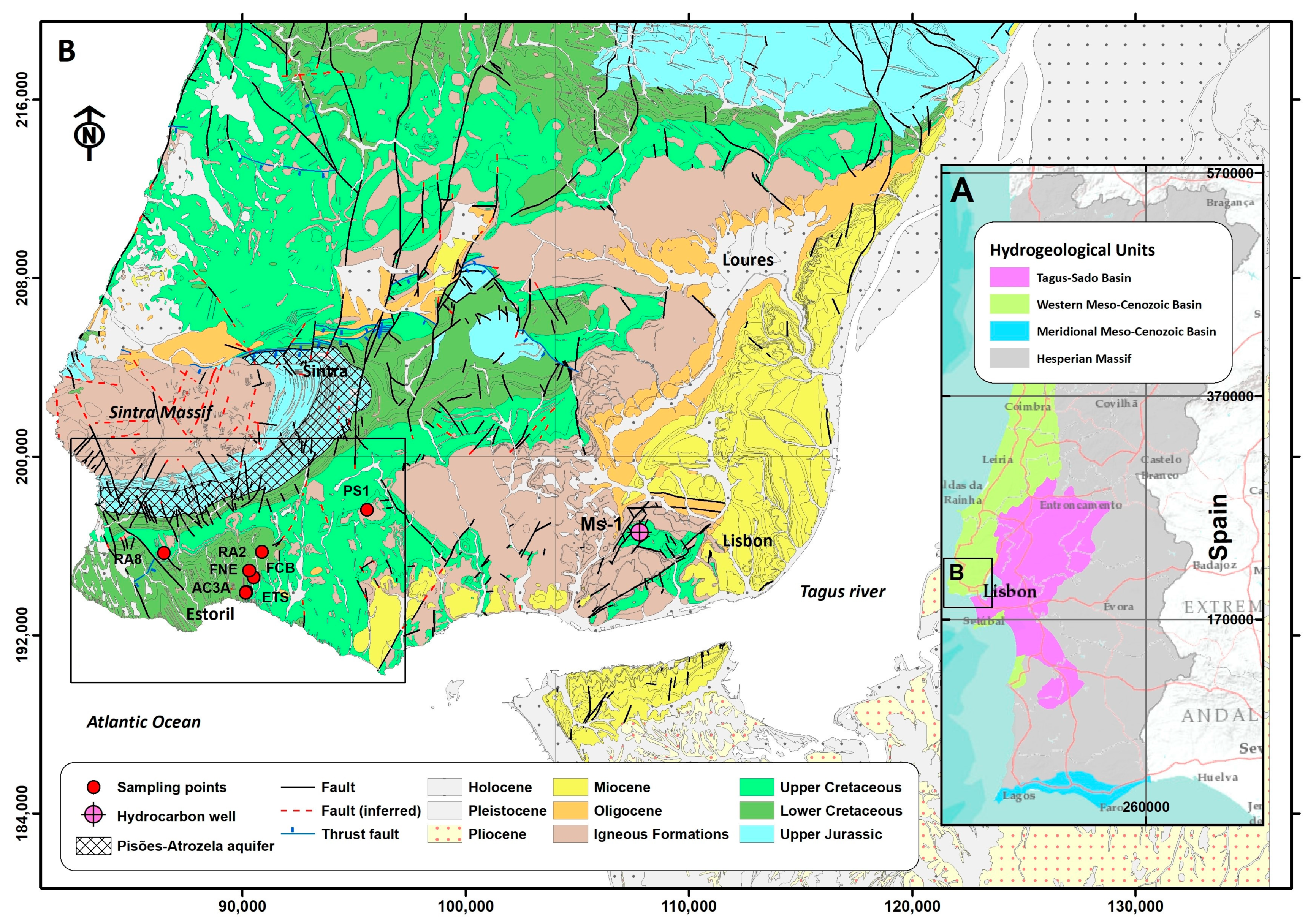
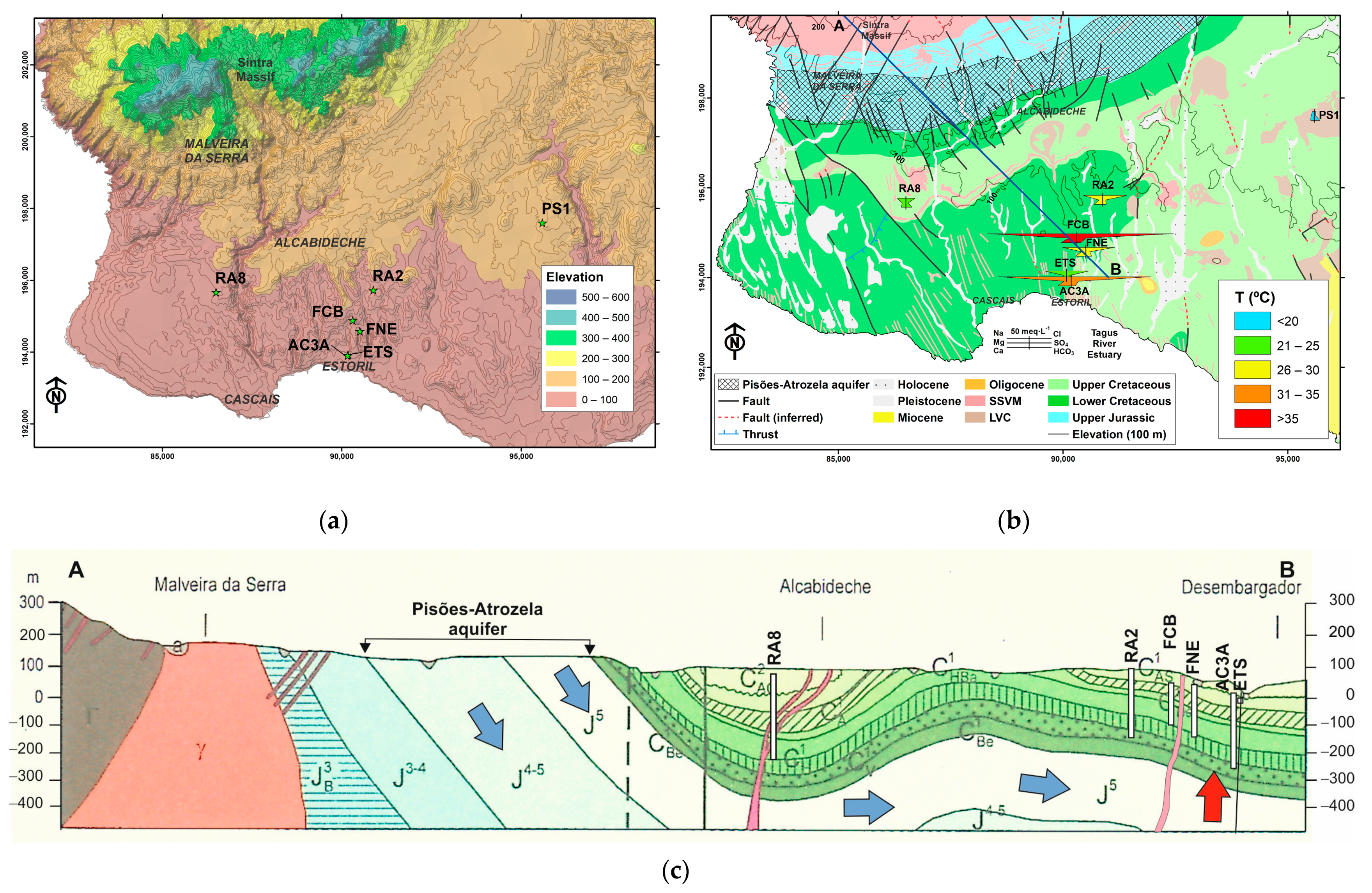
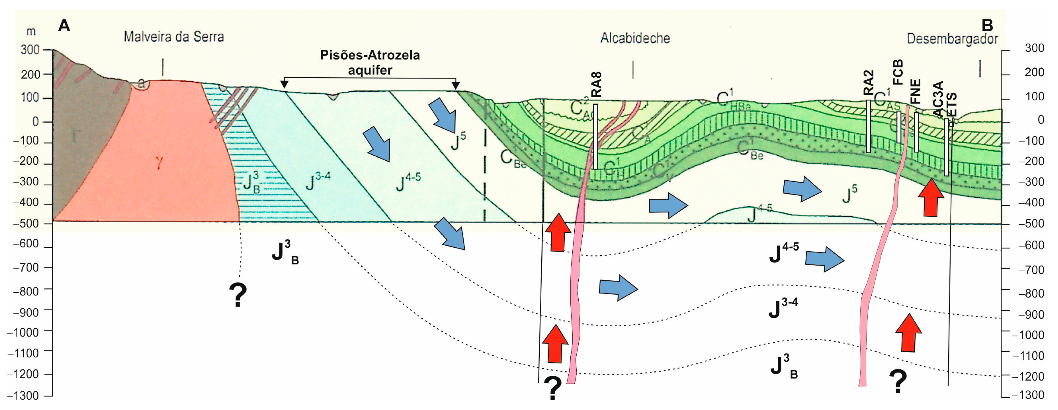
2.2. Geology and Hydrogeological Settings
3. Sampling and Analytical Approach
4. Results and Discussion
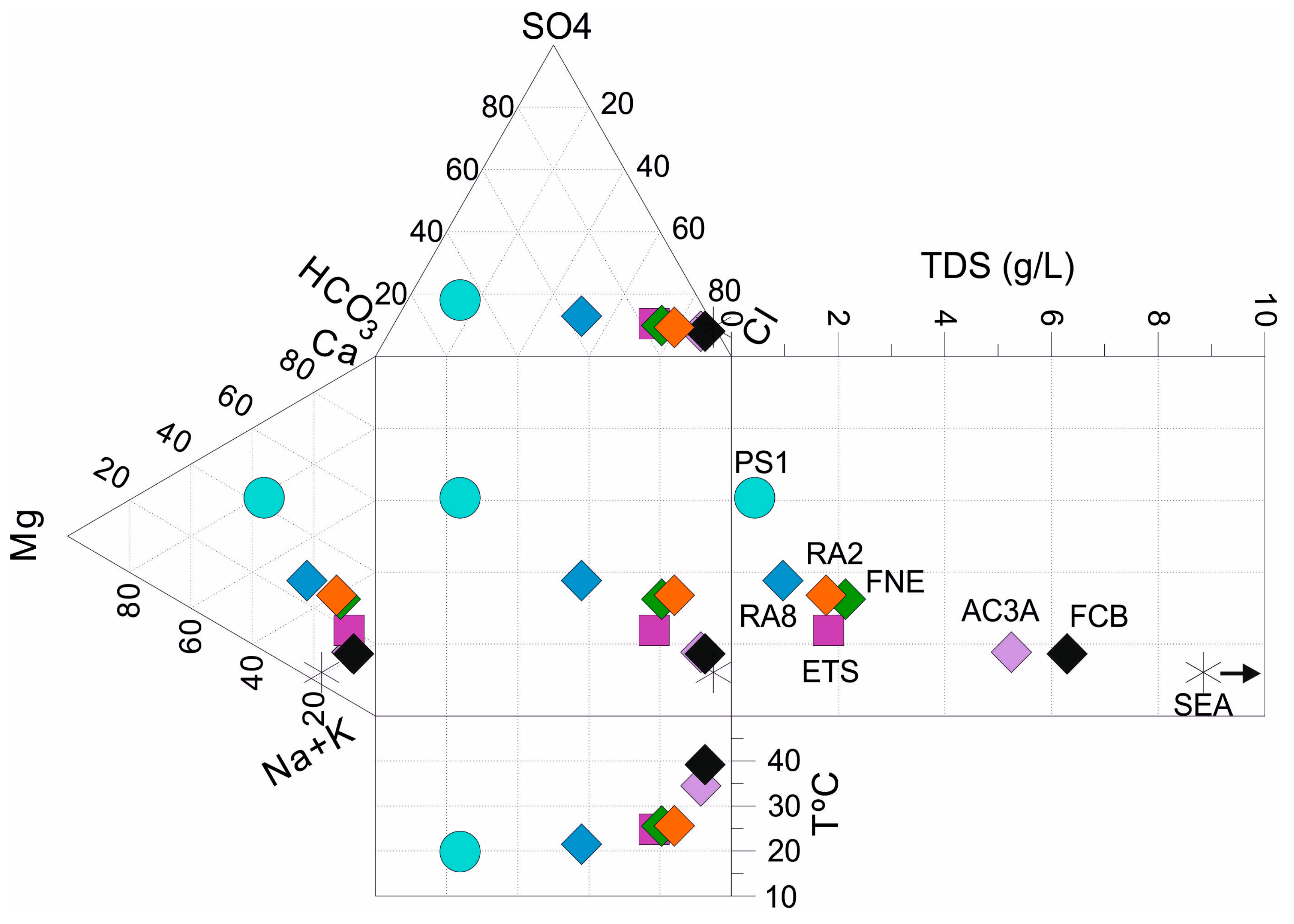
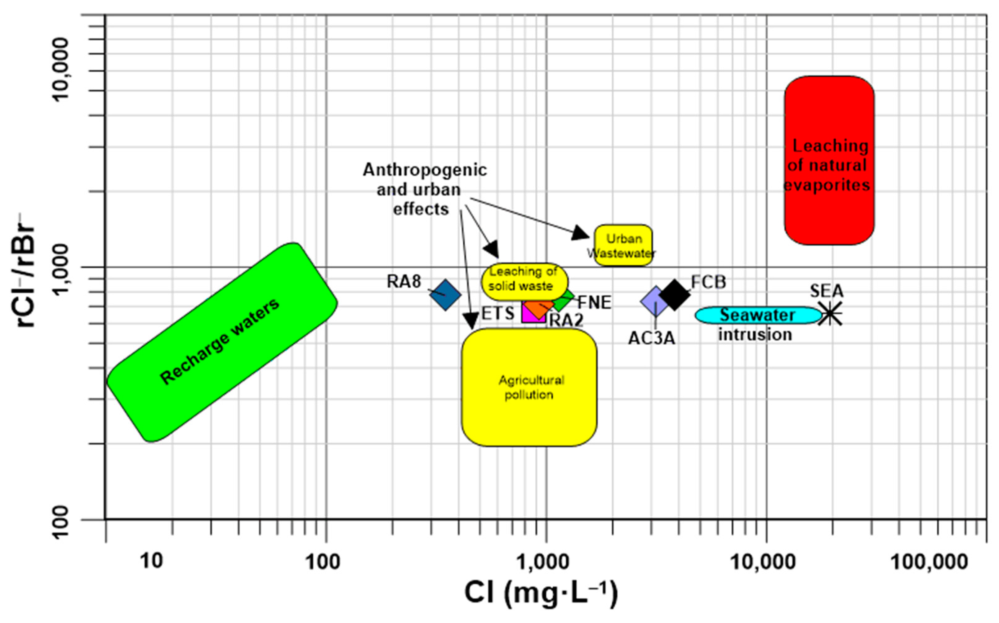
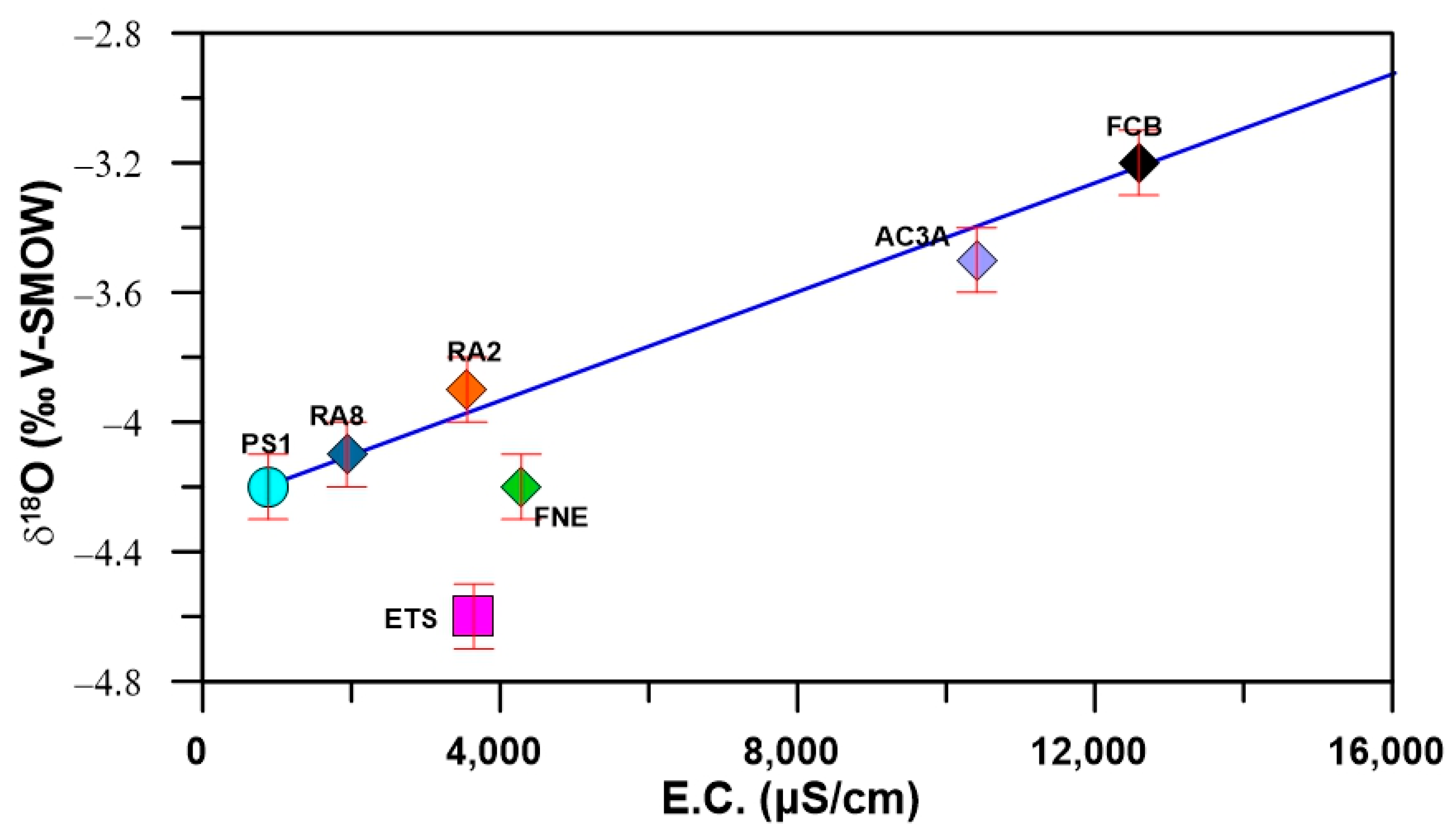
4.1. Groundwater Chemistry

4.2. Environmental Stable and Radioactive Isotopes
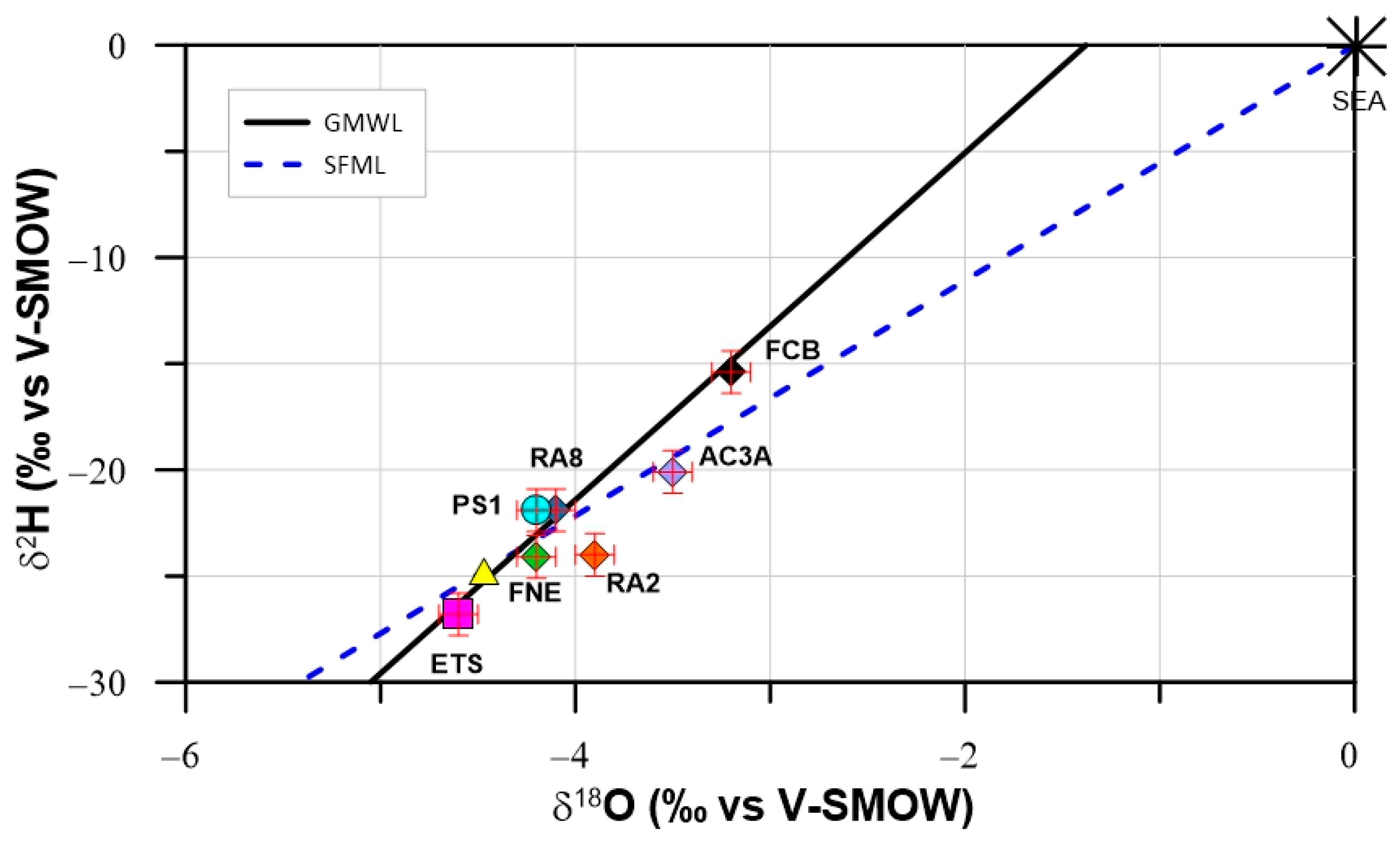
4.2.1. Stable Isotopes
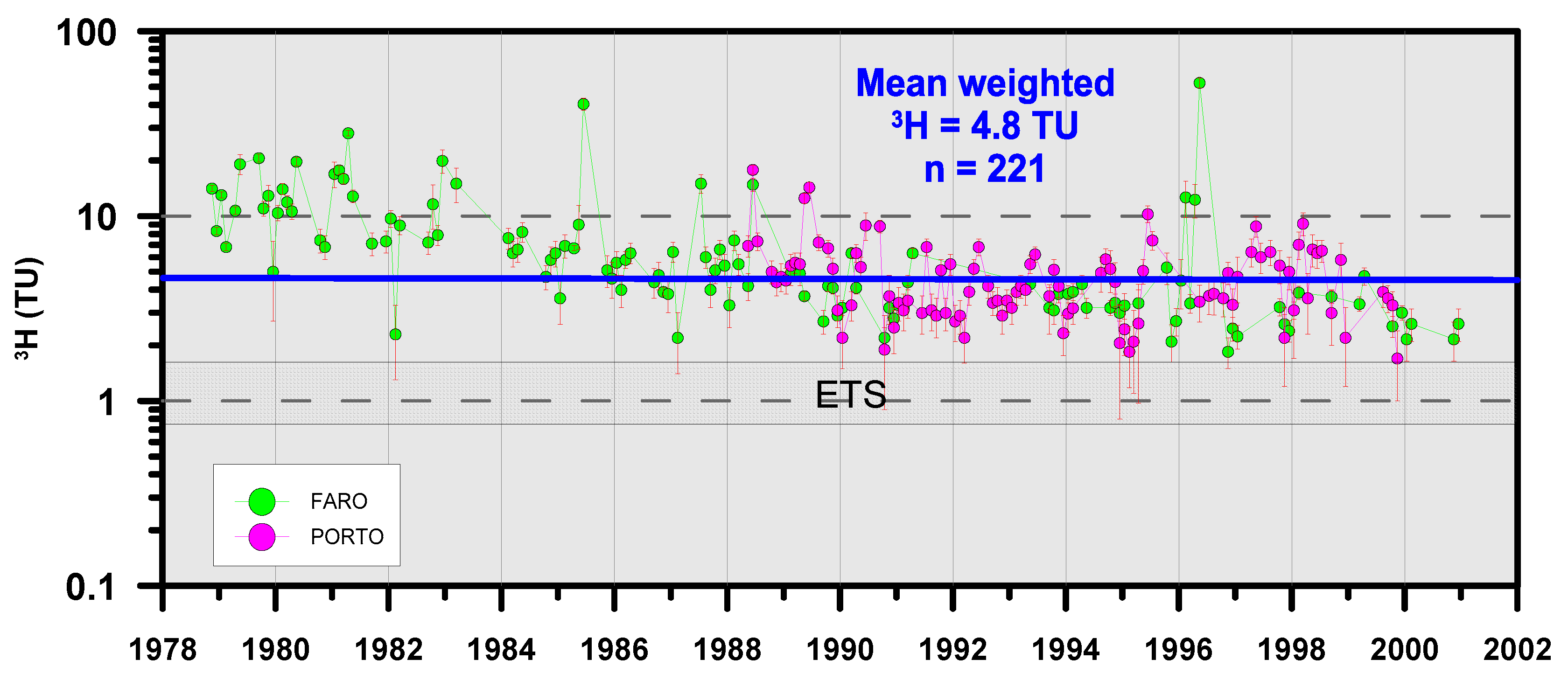
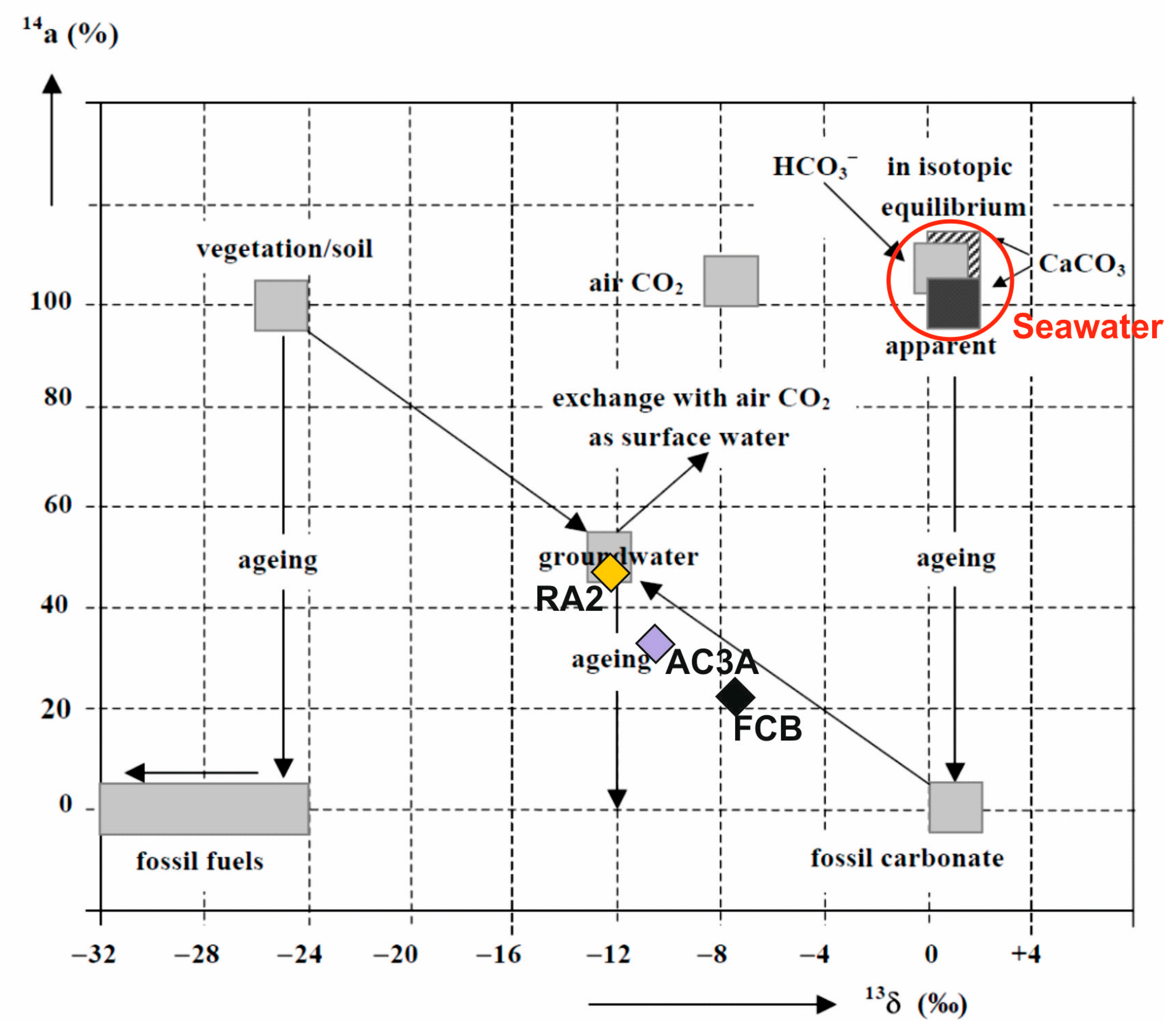
4.2.2. Radioactive Isotopes (3H and 14C)
4.3. Reservoir Settings
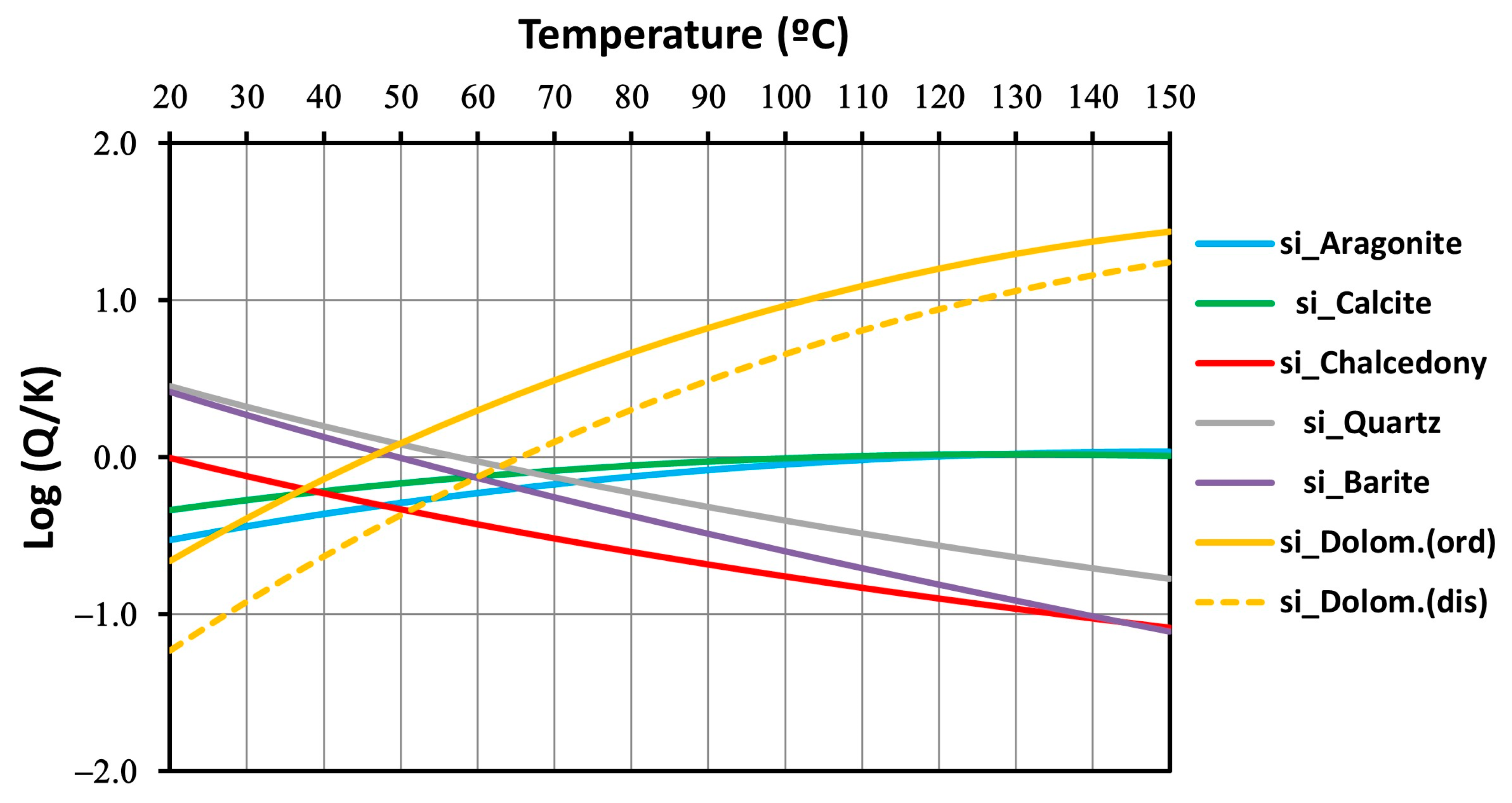
4.3.1. Silica Geothermometers
4.3.2. Marini-Chiodini Graphical Method
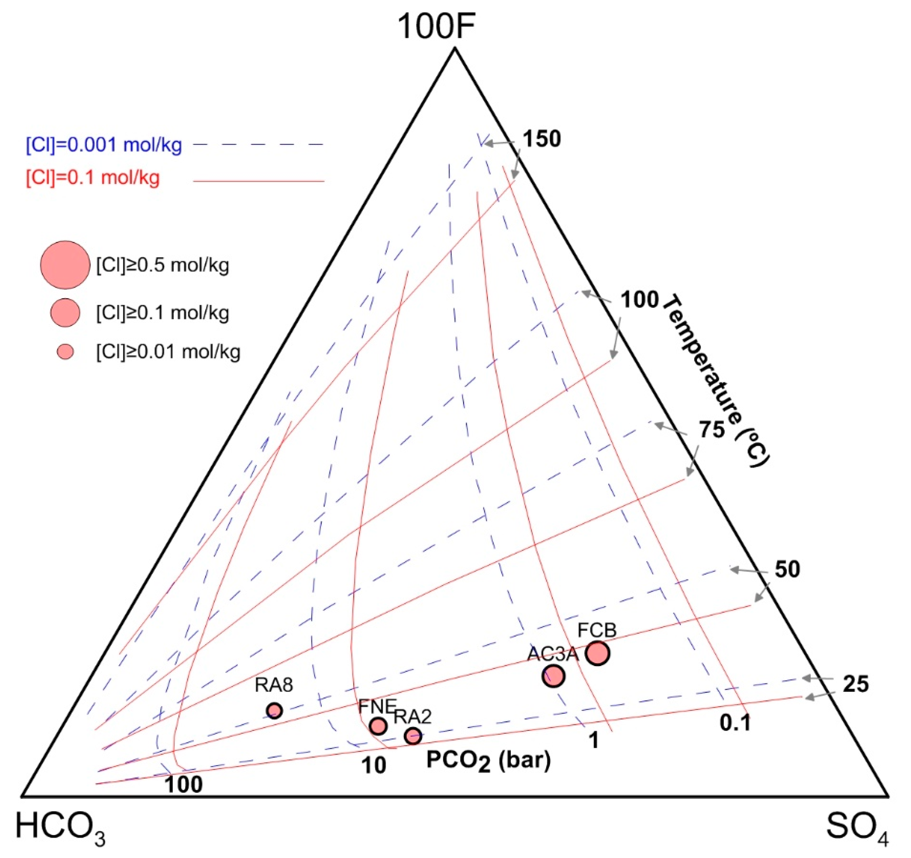
4.3.3. Spycher Graphical Method
4.4. Geochemical Modeling
| Gypsum dissolution | CaSO4·H2O = Ca2+ + SO42− + H2O |
| Halite dissolution: | NaCl = Na+ + Cl− |
| Cation exchange Na+/Ca2+: | Na+ + Ca-X2 = Na-X + Ca2+ |
| Calcite precipitation: | Ca2+ + CO32− = CaCO3 (pp) |
| Dolomite dissolution: | Ca2+ + Mg2+ + CO32− = CaMg(CO3)2 |
5. Conceptual Model Proposed
6. Conclusions
Author Contributions
Funding
Data Availability Statement
Acknowledgments
Conflicts of Interest
References
- Gaye, C.B. Editor’s Message Isotope techniques for monitoring ground water salinization. Hydrog. J. 2001, 9, 217–218. [Google Scholar] [CrossRef]
- Kim, Y.; Lee, K.-S.; Koh, D.-C.; Lee, D.-H.; Lee, S.-G.; Park, W.-B.; Koh, G.-W.; Woo, N.-C. Hydrogeochemical and isotopic evidence of groundwater salinization in a coastal aquifer: A case study in Jeju volcanic island, Korea. J. Hydrol. 2003, 270, 282–294. [Google Scholar] [CrossRef]
- Fidelibus, M.D. Environmental tracing in coastal aquifers: Old problems and new solutions. In Tecnología de la Intrusión de Agua de Mar en Acuíferos Costeros: Países Mediterráneos; Edition: Serie: Hidrogeología y Aguas Subterráneas; López Geta, J.A., de Dios Gómez, J., de la Orden, V., Ramos, G., Rodríguez, L., Eds.; IGME: Madrid, Spain, 2003; Volume 8, pp. 79–111. [Google Scholar]
- Cartwright, I.; Weaver, T.R.; Fifield, L.K. Cl/Br ratios and environmental isotopes as indicators of recharge variability and groundwater flow: An exemple from the southeast Murray Basin, Australia. Chem. Geol. 2006, 231, 38–56. [Google Scholar] [CrossRef]
- Bouchaou, L.; Michelot, J.L.; Vengosh, A.; Hsissou, Y.; Qurtobi, M.; Gaye, C.B.; Bullen, T.D.; Zuppi, M. Application of multiple isotopic and geochemical tracers for investigation of recharge, salinization, and residence time of water in the Souss–Massa aquifer, southwest of Morocco. J. Hydrol. 2008, 352, 267–287. [Google Scholar] [CrossRef]
- Carol, E.; Kruse, E.; Mas-Pla, J. Hydrochemical and isotopical evidence of ground water salinization processes on the coastal plain of Samborombón Bay, Argentina. J. Hydrol. 2009, 365, 335–345. [Google Scholar] [CrossRef]
- Koh, D.-C.; Ha, K.; Lee, K.-S.; Yoon, Y.-Y.; Ko, K.-S. Flow paths and mixing properties of groundwater using hydrogeochemistry and environmental tracers in the southwestern area of Jeju volcanic island. J. Hydrol. 2012, 432–433, 61–74. [Google Scholar] [CrossRef]
- Carreira, P.M. Mechanisms of Salinization of Coastal Aquifers in the Algarve. Master’s Thesis, Universidade Técnica de Lisbon, Lisbon, Portugal, 1991; 143p. (In Portuguese). [Google Scholar]
- Carreira, P.M.; Macedo, M.E.; Soares, A.M.M.; Vieira, M.C.; Santos, J.B. Origin of salinization of the aquifer system of the Lower Sado Basin, in the region of Setubal. Recur. Hídricos 1994, 15, 41–48. (In Portuguese) [Google Scholar]
- Carreira, P.M.; Marques, J.M.; Pina, A.; Mota Gomes, A.; Galego Fernandes, P.A.; Monteiro Santos, F. Groundwater assessment at Santiago Island (Cabo Verde): A multidisciplinary approach to a recurring source of water supply. Water Resour. Manag. 2010, 24, 1139–1159. [Google Scholar] [CrossRef]
- Carreira, P.M.; Marques, J.M.; Nunes, D. Source of groundwater salinity in coastline aquifers based on Environmental isotopes (Portugal): Natural vs. Human interference. A review and reinterpretation. Appl. Geochem. 2014, 41, 163–175. [Google Scholar] [CrossRef]
- Carreira, P.M.; Lobo de Pina, A.; Mota Gomes, A.; Marques, J.M.; Monteiro Santos, F. Radiocarbon dating and stable isotopes content in the assessment of groundwater recharge at Santiago Island, Republic of Cape Verde. Water 2022, 14, 2339. [Google Scholar] [CrossRef]
- Han, D.; Kohfahl, C.; Song, X.; Xiao, G.; Yang, J. Geochemical and isotopic evidence for palaeo-seawater intrusion into the south coast aquifer of Laizhou Bay, China. Appl. Geochem. 2011, 26, 863–883. [Google Scholar] [CrossRef]
- Delgado-Outeiriño, I.; Araujo-Nespereira, P.; Cid-Fernández, J.A.; Mejuto, J.C.; Martínez-Carballo, E.; Simal-Gándara, J. Hydrogeothermal modelling vs. inorganic chemical composition of thermal waters from the area of Carballiño (NW Spain). Hydrol. Earth Syst. Sci. 2012, 16, 157–166. [Google Scholar] [CrossRef] [Green Version]
- Mosaffa, M.; Nazif, S.; Amirhosseini, Y.K.; Balderer, W.; Meiman, H.M. An investigation of the source of salinity in groundwater using stable isotope tracers and GIS: A case study of the Urmia Lake basin, Iran. Groundw. Sustain. Dev. 2021, 12, 100513. [Google Scholar] [CrossRef]
- Hamed, Y.; Ahmadi, R.; Demdoum, A.; Bouri, S.; Gargouri, I.; Dhia, H.B. Use of geochemical, isotopic, and age tracer data to develop models of groundwater flow: A case study of Gafsa mining basin-Southern Tunisia. J. Afr. Earth Sci. 2014, 100, 418–436. [Google Scholar] [CrossRef]
- Hamed, Y.; Zairi, M.; Ali, W.; Dhia, H. Estimation of Residence Times and Recharge Area of Groundwater in the Moulares Mining Basin by Using Carbon and Oxygen Isotopes (South Western Tunisia). J. Environ. Prot. 2010, 1–4, 466–474. [Google Scholar] [CrossRef] [Green Version]
- Tarki, M.; Dassi, L.; Hamed, Y.; Jedoui, Y. Geochemical and isotopic composition of groundwater in the Complex Terminal aquifer in southwestern Tunisia, with emphasis on the mixing by vertical leakage. Environ. Earth Sci. 2011, 64, 85–95. [Google Scholar] [CrossRef]
- Craig, H. Isotopic variations in meteoric waters. Science 1961, 133, 1702–1703. [Google Scholar] [CrossRef]
- Dansgaard, W. Stable isotopes in precipitation. Tellus 1964, 16, 436–468. [Google Scholar] [CrossRef]
- Rozanski, K.; Araguás-Araguás, L.; Gonfiantini, R. Relation between long-term of oxygen-18 isotope composition of precipitation and climate. Science 1992, 258, 981–985. [Google Scholar] [CrossRef]
- Gourcy, L.L.; Groening, M.; Aggarwal, P.K. Stable oxygen and hydrogen isotopes in precipitation. In Isotopes in the Water Cycle; Aggarwal, P.K., Gat, J.R., Froehlich, K.F.O., Eds.; Springer: Dordrecht, The Netherlands, 2005; pp. 39–51. [Google Scholar] [CrossRef]
- Terzer, S.; Wassenaar, L.I.; Aráguas-Aráguas, L.J.; Aggarwal, P.K. Global isoscapes for δ18O and δ2H in precipitation: Improved prediction using regionalized climatic regression models. Hydrol. Earth Syst. Sci. 2013, 17, 4713–4728. [Google Scholar] [CrossRef]
- Vystavna, Y.; Matiatos, I.; Wassenaar, L.I. Temperature and precipitation effects on the isotopic composition of global precipitation reveal long-term climate dynamics. Sci. Rep. 2021, 11, 18503. [Google Scholar] [CrossRef] [PubMed]
- Carreira, P.M.; Marques, J.M.; Graça, R.; Aires-Barros, L. Radiocarbon application in dating “complex” hot and cold CO2-rich mineral water systems: A review of case studies ascribed to the northern Portugal. Appl. Geochem. 2008, 23, 2817–2828. [Google Scholar] [CrossRef]
- Lucas, L.L.; Unterweger, M.P. Comprehensive review and critical evaluation of the half-life of tritium. J. Res. Natl. Inst. Stand. Technol. 2000, 105, 541–549. [Google Scholar] [CrossRef] [PubMed]
- Mook, W.G. Environmental Isotopes in the Hydrological Cycle: Principles and Applications; IAEA: Vienna, Austria, 2000; 596p. [Google Scholar]
- Edmunds, W. Groundwater as an Archive of Climatic and Environmental Change. In Isotopes in the Water Cycle; Aggarwal, P.K., Gat, J.R., Froehlich, K.F., Eds.; Springer: Dordrecht, The Netherlands, 2005; pp. 341–352. [Google Scholar] [CrossRef]
- Schwarcz, H.P.; Cortecci, G. Isotopic analyses of spring and stream water SO4 from the Italian Alps and Apennines. Chem. Geol. 1974, 13, 285–294. [Google Scholar] [CrossRef]
- Krouse, H.R.; Mayer, B. Sulphur and oxygen isotopes in sulphate. In Environmental Tracers in Subsurface Hydrology; Cook, P.G., Herczeg, A.L., Eds.; Springer: Boston, MA, USA, 2000; pp. 195–231. [Google Scholar] [CrossRef]
- Gattacceca, J.C.; Vallet-Coulomb, C.; Mayer, A.; Claude, C.; Radakovitch, O.; Conchetto, E.; Hamelin, B. Isotopic and geochemical characterization of salinization in the shallow aquifers of a reclaimed subsiding zone: The southern venice lagoon coastland. J. Hydrol. 2009, 378, 46–61. [Google Scholar] [CrossRef]
- Mongelli, G.; Monni, S.; Oggiano, G.; Paternoster, M.; Sinisi, R. Tracing groundwater salinization processes in coastal aquifers: A hydrogeochemical and isotopic approach in the Na-Cl brackish waters of northwestern Sardinia, Italy. Hydrol. Earth Syst. Sci. 2013, 17, 2917–2928. [Google Scholar] [CrossRef] [Green Version]
- Marques, J.M.; Eggenkamp, H.G.M.; Graça, H.; Carreira, P.M.; Matias, M.J.; Mayer, B.; Nunes, D. Assessment of recharge and flowpaths in a limestone thermomineral aquifer system using environmental isotope tracers (Central Portugal). Isotopes Environ. Health Stud. 2010, 46, 156–165. [Google Scholar] [CrossRef]
- Acciaiuoli, L. Le Portugal Hydromineral; Direction Génèrale dês Mines e dês Services Geologiques: Lisbon, Portugal, 1952; Volume 6, 284p. (In French) [Google Scholar]
- Ramalho, M.M.; Rey, J.; Zbyszewski, G.; Matos, C.A.A.; Moitinho de Almeida, F.; Costa, C.; Carla, M.K. Notícia explicativa da Carta Geológica de Portugal, folha 34-C - Cascais; Serviços Geológicos de Portugal: Lisbon, Portugal, 1981; 87p. [Google Scholar]
- Lopo-Mendonça, J.; Oliveira da Silva, M.; Bahir, M. Considerations concerning the origin of the Estoril (Portugal) thermal water. Estud. Geológicos 2004, 60, 153–159. [Google Scholar]
- Jesus, M.R. Contaminação em aquíferos carbonatados na região de Lisboa-Sintra-Cascais. Master’s Thesis, Universidade de Lisboa, Lisbon, Portugal, 1995. [Google Scholar]
- Ramalho, M.M.; Rey, J.; Zbyszewski, G.; Matos Alves, C.A.; Palácios, T.; Moitinho De Almeida, F.; Costa, C.; Kullberg, M.C. Carta e Notícia Explicativa da Folha 34-C Cascais; IGM: Lisbon, Portugal, 2001; 104p. [Google Scholar]
- Almeida, C.; Mendonça, J.J.L.; Jesus, M.R.; Gomes, A.J. Sistemas Aquíferos de Portugal Continental; Centro de Geologia da Faculdade de Ciências de Lisboa; Instituto Nacional da Água: Lisbon, Portugal, 2000; Volume II, 139p. [Google Scholar] [CrossRef]
- LNEG, Carta Geológica de Portugal 1:50,000—Sheets 34A (1993), 34B (2011), 34C (1999), 34D (2006). National Laboratory of Energy and Geology: Lisbon, Portugal; Available online: https://eurogeologists.eu/wp-content/uploads/2017/12/EGJ44_lr-1.pdf#page=32 (accessed on 20 December 2022).
- Rasmussen, E.S.; Lomholt, S.; Andersen, C.; Vejbaek, O.V. Aspects of the structural evolution of the Lusitanian Basin in Portugal and the shelf and slope area offshore Portugal. Tectonophysics 1998, 300, 199–225. [Google Scholar] [CrossRef]
- Dias, R.; Araújo, A.; Terrinha, P.; Kullberg, J.C. (Eds.) Geologia de Portugal, Vol. II, Geologia Meso-Cenozóica de Portugal (Geology of Portugal, Vol. II, Meso-Cenozoic Geology of Portugal); Escolar Editora: Lisboa, Portugal, 2013; pp. 195–347. [Google Scholar]
- Carvalho, J.; Lopo-Mendonça, J.; Berthou, P.Y.; Blanc, P. Etude geologique et hydrogeologique des forages d’Estoril. In III Semana de Hidrogeologia; Departamento de Geologia e Centro de Geologia, Faculdade de Ciencias: Lisbon, Portugal, 1982; pp. 379–438. [Google Scholar]
- Andrade, C.F. A tectónica do estuário do Tejo e dos vales submarinos ao largo da costa da Caparica, e a sua relação com as nascentes termo-medicinais de Lisboa (Considerações Preliminares). Comun. Dos Serviços Geológicos De Port. 1933, 19, 21. [Google Scholar]
- Almeida, A. Lisboa, Capital das Águas. Rev. Munic. 1952, 49–50, 27. [Google Scholar]
- Almeida, C.; Carvalho, M.R.; Almeida, S. Modelação de Processos Hidrogeoquímicos Ocorrentes nos Aquíferos Carbonatados da Região de Lisoba-Cascais-Sintra. Hidrogeol. Recur. Hidráulicos 1991, 18, 289–304. [Google Scholar]
- Seifert, H. Águas Termais de Estoril: Avaliação do seu Potencial com Vista ao Abastecimento das Piscinas Termais Projectadas Pela Sociedade Estoril Plage; internal report; Gabinete de Estudos Geológicos e Hidrológicos Lda: Lisbon, Portugal, 1965; 15p. [Google Scholar]
- Ferreira, F.; Carvalho, M.R.; Silva, C.; Almeida, C. Variabilidade hidrogeoquímica nos aquíferos carbonatados entre Lisboa e Cascais. In Proceedings of the VIII Seminário Sobre Águas Subterrâneas, Lisbon, Portugal, 10–11 March 2011. [Google Scholar]
- Clark, I.D.; Fritz, P. Environmental Isotopes in Hydrogeology, 1st ed.; CRC Press: Boca Raton, CA, USA, 1997. [Google Scholar] [CrossRef]
- IAEA. Procedure and Technique Critique for Tritium Enrichment by Electrolysis at IAEA Laboratory; Technical Procedure 19; internal report; IAEA-IHS Laboratories: Vienna, Austria, 1976. [Google Scholar]
- IAEA. Sampling of Water for 14C Analysis; IAEA-IHS Laboratories: Vienna, Austria, 1981. [Google Scholar]
- Giesemann, A.; Jaeger, H.-J.; Norman, A.L.; Krouse, H.R.; Brand, W.A. Online Sulfur-Isotope Determination Using an Elemental Analyzer Coupled to a Mass Spectrometer. Anal. Chem. 1994, 66, 2816–2819. [Google Scholar] [CrossRef]
- Parkhurst, D.L.; Appelo, C.A.J. Description of input and examples for PHREEQC version 3—A computer program for speciation, batch-reaction, one-dimensional transport, and inverse geochemical calculations. In U.S. Geological Survey Techniques and Methods; U.S. Geological Survey: Denver, CO, USA, 2013; Chapter A43; 497p. Available online: http://pubs.usgs.gov/tm/06/a43/ (accessed on 20 December 2022).
- Alcalá, F.J.; Custodio, E. Using the Cl/Br ratio as a tracer to identify the origin of salinity in aquifers in Spain and Portugal. J. Hydrol. 2008, 359, 189–207. [Google Scholar] [CrossRef]
- Carvalho, M.R.; Carreira, P.M.; Silva, M.C.R.; Vieira da Silva, A.; Nunes, D. Geochemical and isotopes approach on the characterization of groundwater paths in Sintra Massive (Portugal). In Proceedings of the Goldschmidt Conference 2009, Davos, Switzerland, 21–26 June 2009; p. A196. [Google Scholar]
- Morais, M.; Recio, C. Geochemical and isotopic controls of carbon and sulphur in calciumsulphate waters of the western Meso-Cenozoic Portuguese border (natural mineral waters of Curia and Monte Real). In Advances in the Research of Aquatic Environment; Lambrakis, N., Stournaras, G., Katsanou, K., Eds.; Environmental Earth Sciences; Springer: Berlin/Heidelberg, Germany, 2011; pp. 125–133. [Google Scholar] [CrossRef] [Green Version]
- Kendal, C.; McDonnell, J.J. Isotope Tracers in Catchment Hydrology; Elsevier: Amsterdam, The Netherlands, 1998; 839p, ISBN 978-0-444-81546-0. [Google Scholar]
- Carvalho, M.R.; Ferreira, F.; Silva, C.; Almeida, C. Origin of Dissolved Carbon in Groundwaters from Carbonated Aquifers in Lisbon-Cascais Region (Portugal) Using δ13C; AIG10: Budapest, Hungary, 2013. [Google Scholar]
- Vogel, J.C. Carbon-14 dating of groundwater. In Proceedings of the Symposium on Use of Isotopes in Hydrology (IAEA-SM—129/15), Vienna, Austria, 9–13 March 1970; pp. 225–237. [Google Scholar]
- Geyh, M.A. Basic studies in hydrology and 14C and 3H measurements. In Proceedings of the 24th International Geology Congress, Montreal, QC, Canada, 1972; International Geological Congress: Montreal, QC, Canada, 1972; Volume 11, pp. 227–234. [Google Scholar]
- Gonfiantini, R.; Zuppi, G.M. Carbon isotope exchange rate of DIC in karst groundwater. Chem. Geol. 2003, 197, 319–336. [Google Scholar] [CrossRef]
- Criss, R.; Davisson, L.; Surbeck, H.; Winston, W. Isotopic methods. In Methods in Karst Hydrogeology: IAH: International Contributions to Hydrogeology, 26, 1st ed.; Goldscheider, N., Drew, D., Eds.; CRC Press: London, UK, 2007; pp. 123–145. [Google Scholar] [CrossRef]
- Chiodini, G.; Frondini, F.; Marini, L. Theoretical geothermometers and PCO2 indicators for aqueous solutions coming from hydrothermal systems of medium-low temperature hosted in carbonate-evaporite rocks. Application to the thermal springs of the Etruscan Swell, Italy. Appl. Geochem. 1995, 10, 337–346. [Google Scholar] [CrossRef]
- Sonney, R.; Vuataz, F.-D. Validation of Chemical and Isotopic Geothermometers from Low Temperature Deep Fluids of Northern Switzerland. In Proceedings of the 2010 World Geothermal Congress, Bali, Indonesia, 25–30 April 2010; Available online: http://doc.rero.ch/record/29458 (accessed on 20 December 2022).
- Fournier, R.O. Chemical geothermometers and mixing models for geothermal systems. Geothermics 1977, 5, 41–50. [Google Scholar] [CrossRef]
- Marini, L.; Chiodini, G.; Cioni, R. New Geothermometers for carbonate-evaporite geothermal reservoirs. Geothermics 1986, 15, 77–86. [Google Scholar] [CrossRef]
- Spycher, N.; Peiffer, L.; Sonnenthal, E.L.; Saldi, G.; Reed, M.H.; Kennedy, B.M. Integrated multicomponent solute geothermometry. Geothermics 2014, 51, 113–123. [Google Scholar] [CrossRef]
- Ramalho, E.C. Sondagens Mecânicas e Prospecção Geofísica na Caracterização de Fluidos. Ph.D. Thesis, Universidade de Aveiro, Portugal, Spain, 2013; 186p. [Google Scholar]
- Marrero-Diaz, R.; Ramalho, E.; Costa, A.; Ribeiro, L.; Carvalho, J.; Pinto, C.; Rosa, D.; Correia, A. Updated Geothermal Assessment of Lower Cretaceous Aquifer in Lisbon Region, Portugal. In Proceedings of the World Geothermal Congress 2015, Melbourne, Australia, 19–25 April 2015. Extended abstract 16012. [Google Scholar]
- Alves, J.F. Analise de Viabilidade de Armazenamento de Energia sob a Forma de ar Comprimido em Cavernas Subterrâneas. Master’s Thesis, Universidade de Évora, Évora, Portugal, 2015. [Google Scholar]


| Name | Flow | Elevation | Depth | Screen Depth | Date | Air T. | Water T. | pH | E.C. | TDS | SiO2 | Ca2+ | Mg2+ | Na+ | K+ | HCO3− | Cl− | SO42− | NO3− | Br− | IBE |
| Unit | L/s | m a.s.l | m | Initial(m)/Final(m) | mm-yy | °C | °C | µS/cm (@25°C) | g/L | mg/L | mg/L | mg/L | mg/L | mg/L | mg/L | mg/L | mg/L | mg/L | mg/L | % | |
| PS1 | 22.5 | 119 | 395 | 74/334 | 06-13 | 23 | 19.9 | 7.40 | 880 | 0.7 | 13.0 | 82.0 | 42.2 | 43.3 | 6.6 | 385.0 | 49.0 | 81.1 | 2.7 | n.d. | 1.7 |
| RA8 | 5.0 | 98 | 300 | unk. | 06-13 | 25 | 21.5 | 7.32 | 1937 | 1.0 | 14.8 | 102.3 | 52.3 | 219.7 | 12.1 | 414.3 | 347.1 | 117.3 | 0.4 | 1.0 | 1.2 |
| RA2 | 22.2 | 98 | 246 | 102/198 | 01-14 | 23 | 26.7 | 6.98 | 3558 | 1.8 | 15.7 | 194.0 | 54.7 | 484.0 | 13.2 | 230.0 | 931.0 | 147.0 | 5.1 | 2.9 | 3.6 |
| ETS | 1.0 | 31 | 0 | - | 01-14 | 23 | 24.8 | 7.86 | 3647 | 1.8 | 21.2 | 133.0 | 35.5 | 551.0 | 18.3 | 341.0 | 879.0 | 170.0 | 15.3 | 2.8 | 0.1 |
| FCB | unk. | 67 | 110 | unk. | 01-14 | 14 | 39.2 | 7.18 | 12,590 | 6.3 | 36.0 | 347.3 | 109.0 | 2255.0 | 68.6 | 251.0 | 3831.0 | 469.0 | 2.9 | 11.0 | 1.6 |
| FNE | unk. | 59 | 170 | unk. | 12-13 | 15 | 25.6 | 6.87 | 4286 | 2.1 | 21.6 | 227.9 | 58.9 | 594.6 | 14.6 | 378.2 | 1133.0 | 200.3 | 8.5 | 3.3 | 0.1 |
| AC3A | 15.4 | 31 | 279 | 135/267 | 12-13 | 17 | 32.5 | 6.96 | 10,410 | 5.2 | 29.3 | 287.0 | 97.5 | 1826.0 | 56.3 | 285.3 | 3136.4 | 391.6 | 2.3 | 9.6 | 0.9 |
| SEA * | - | - | - | - | - | - | - | - | 160,000 | 34.5 | 10 | 411 | 1290 | 10,760 | 399 | 142 | 19,350 | 2710 | 2 | 67 | 0 |
| Name | Cl−/Br− | Na+/Cl− | Seawater contribution (%) | Anhydrite | Aragonite | Calcite | Dolomite | Gypsum | Halite | Quartz | Chalcedony | ||||||||||
| Unit | molar | molar | Cl | δ18O | SI | SI | SI | SI | SI | SI | SI | SI | |||||||||
| PS1 | - | 1.35 | 0.0 | 0.0 | −1.98 | 0.18 | 0.38 | 0.18 | −1.71 | −7.28 | 0.4 | −0.10 | |||||||||
| RA8 | 782 | 0.98 | 1.5 | 2.4 | −1.58 | −0.24 | −0.06 | −0.85 | −1.34 | −5.02 | 0.41 | 0.00 | |||||||||
| RA2 | 724 | 0.80 | 4.6 | 7.1 | −1.84 | 0.08 | 0.27 | −0.01 | −1.57 | −5.75 | 0.45 | 0.00 | |||||||||
| ETS | 682 | 0.97 | 4.3 | −9.5 | −1.66 | 0.62 | 0.8 | 0.85 | −1.41 | −4.99 | 0.55 | 0.10 | |||||||||
| FCB | 785 | 0.91 | 19.6 | 23.8 | −1.14 | 0.22 | 0.37 | 0.29 | −0.96 | −3.84 | 0.62 | 0.20 | |||||||||
| FNE | 774 | 0.81 | 5.6 | 0.0 | −1.44 | −0.1 | 0.07 | −0.62 | −1.19 | −4.86 | 0.55 | 0.10 | |||||||||
| AC3A | 736 | 0.90 | 16.0 | 16.7 | −1.25 | −0.07 | 0.09 | −0.35 | −1.04 | −3.99 | 0.61 | 0.20 | |||||||||
| SEA * | 655 | 0.86 | 100 | 100 | |||||||||||||||||
| Name | δ18OH2O | δ2HH2O | Deuterium Excess (d) | δ34SSO4 | δ18OSO4 | Recharge Altitude |
|---|---|---|---|---|---|---|
| Unit | ‰ V-SMOW (±0.05) | ‰ V-SMOW (±1.0) | ‰ V-SMOW | ‰ V-CDT (±0.3) | ‰ V-SMOW (±0.6) | m a.s.l. |
| PS1 | −4.2 | −21.9 | 11.7 | n.a. | n.a. | 447 |
| RA8 | −4.1 | −21.9 | 10.9 | n.a. | n.a. | 447 |
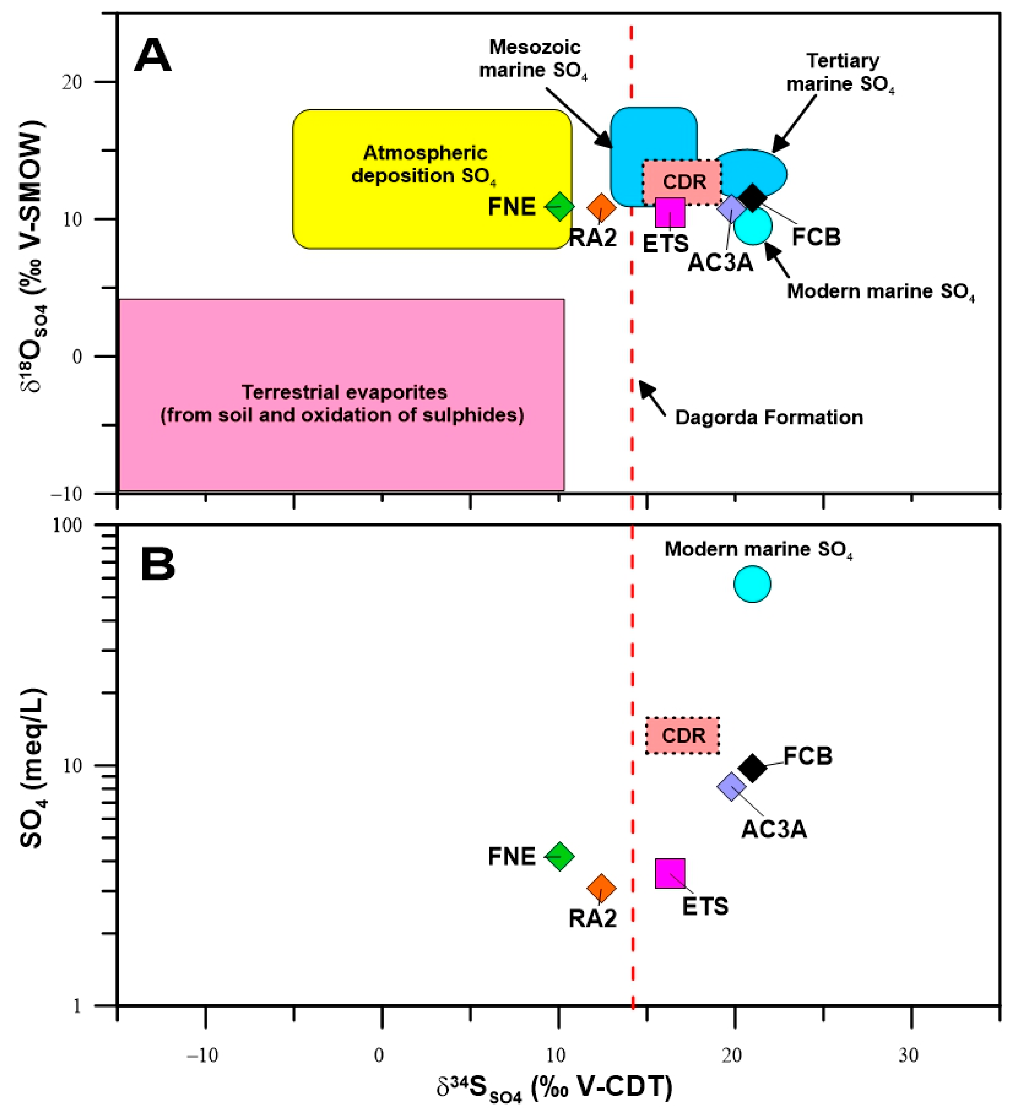
| RA2 | −3.9 | −24.0 | 7.2 | +12.4 | +10.8 | - |
| ETS | −4.6 | −26.8 | 10 | +16.3 | +10.5 | - |
| FCB | −3.2 | −15.4 | 10.2 | +21.0 | +11.5 | - |
| FNE | −4.2 | −24.1 | 9.5 | +10.1 | +10.9 | - |
| AC3A | −3.5 | −20.1 | 7.9 | +19.8 | +10.7 | - |
| SEA* | 0.0 | 0.0 | 0.0 | +20.0 | +9.5 | - |
| Sample ID | 3H | δ13CTDIC | a14C | a14C (C0) | 14C Apparent Age ± 2σ | ||
|---|---|---|---|---|---|---|---|
| δS = −27‰ | δS = −25‰ | δS = −23‰ | |||||
| Unit | TU (±0.6) | ‰ V-PDB (±0.1) | pMC | pMC | ka | ka | ka |
| PS1 | n.a. | n.a. | n.a. | n.a. | n.a. | n.a. | n.a. |
| RA8 | n.a. | n.a. | n.a. | n.a. | n.a. | n.a. | n.a. |
| ETS | 1.2 | n.a. | n.a. | n.a. | n.a. | n.a. | n.a. |
| FNE | b.d.l. | n.a. | n.a. | n.a. | n.a. | n.a. | n.a. |
| RA2 | b.d.l. | −11.7 | 52.67 ± 0.7 | 100 | 1.75 ± 1.00 | 2.70 ± 1.06 | 3.78 ±1.14 |
| 85 | 0.43 ± 1.77 | 1.38 ± 1.84 | 2.47 ± 1.95 | ||||
| 65 | Modern | Modern | 0.30 ± 1.14 | ||||
| FCB | b.d.l. | −7.51 | 22.20 ± 0.3 | 100 | 5.22 ± 1.31 | 6.18 ± 1.36 | 7.26 ± 1.42 |
| 85 | 3.90 ± 2.44 | 4.86 ± 2.50 | 5.94 ± 2.58 | ||||
| 65 | 1.74 ± 1.31 | 2.69 ± 1.36 | 3.78 ± 1.42 | ||||
| AC3A | b.d.l. | −10.7 | 28.69 ± 0.4 | 100 | 6.03 ± 1.05 | 6.98 ± 1.11 | 8.07 ± 1.18 |
| 85 | 4.71 ± 1.87 | 5.67 ± 1.95 | 6.75 ± 2.05 | ||||
| 65 | 2.54 ± 1.05 | 3.50 ± 1.11 | 4.58 ± 1.18 | ||||
| Name | Silica (Quartz) | Silica (Chalcedony) | Marini-Chiodini | Spycher | Reservoir Depth |
|---|---|---|---|---|---|
| Unit | °C | °C | °C | °C | Min–Max (m) |
| RA8 | 52 | n.d. | 75 | n.d. | 1522–2522 |
| RA2 | 55 | n.d. | 45 | 61 | 1217–1913 |
| FCB | 87 | 56 | 65 | 39 | 1435–3043 |
| FNE | 66 | 34 | 55 | 57 | 1652–2130 |
| AC3A | 78 | 47 | 60 | 48 | 1348–2652 |
| Name | pH | Alkalinity | Si | Ca2+ | Mg2+ | Na+ | K+ | Cl− | SO42− | F− | Br− |
|---|---|---|---|---|---|---|---|---|---|---|---|
| RA2 | 6.98 | 3.8 × 10⁻³ | 2.6 × 10⁻⁴ | 4.9 × 10⁻³ | 2.3 × 10⁻³ | 2.1 × 10⁻² | 3.4 × 10⁻⁴ | 2.6 × 10⁻² | 1.5 × 10⁻³ | 5.8 × 10⁻⁶ | 3.6 × 10⁻⁵ |
| Seawater | 8.22 | 2.3 × 10⁻³ | 1.7 × 10⁻⁴ | 1.0 × 10⁻² | 5.3 × 10⁻² | 4.7 × 10⁻¹ | 1.0 × 10⁻² | 5.5 × 10⁻¹ | 2.8 × 10⁻² | 6.8 × 10⁻⁵ | 8.4 × 10⁻⁴ |
| Mix | 7.09 | 3.6 × 10⁻³ | 2.5 × 10⁻⁴ | 5.7 × 10⁻³ | 1.0 × 10⁻² | 9.3 × 10⁻² | 1.9 × 10⁻³ | 1.1 × 10⁻¹ | 5.8 × 10⁻³ | 1.6 × 10⁻⁵ | 1.7 × 10⁻⁴ |
| Mix+ Diss. | 7.04 | 4.1 × 10⁻³ | 6.0 × 10⁻⁴ | 1.2 × 10⁻² | 4.5 × 10⁻³ | 9.3 × 10⁻² | 1.9 × 10⁻³ | 1.1 × 10⁻¹ | 5.8 × 10⁻³ | 1.6 × 10⁻⁵ | 1.7 × 10⁻⁴ |
| FCB | 7.18 | 4.1 × 10⁻³ | 6.0 × 10⁻⁴ | 8.7 × 10⁻³ | 4.5 × 10⁻³ | 9.9 × 10⁻² | 1.8 × 10⁻³ | 1.1 × 10⁻¹ | 4.9 × 10⁻³ | 3.3 × 10⁻⁵ | 1.4 × 10⁻⁴ |
| Inv. Model | Calcite | Chalcedony | CO2 (g) | Dolomite | Forsterite | Gypsum | Halite | Sylvite | CaX2 | NaX |
| Model 1 | −4.3 × 10⁻³ | 2.3 × 10⁻⁴ | 0.0× 100 | 2.2 × 10⁻³ | 4.5 × 10⁻⁵ | 3.4 × 10⁻³ | 8.4 × 10⁻² | 1.4 × 10⁻³ | 2.6 × 10⁻³ | −5.3 × 10⁻³ |
| Model 2 | −3.7 × 10⁻³ | 0.0E+00 | 5.9 × 10⁻⁴ | 1.6 × 10⁻³ | 3.4 × 10⁻⁴ | 3.4 × 10⁻³ | 8.4 × 10⁻² | 1.4 × 10⁻³ | 2.6 × 10⁻³ | −5.3 × 10⁻³ |
| React Path | pH | Alkalinity | Si | Ca2+ | Mg2+ | Na+ | K+ | Cl− | SO42− | |
| RA2 | 6.98 | 3. 8 × 10⁻³ | 2.6 × 10⁻⁴ | 4.9 × 10⁻³ | 2.3 × 10⁻³ | 2.1 × 10⁻² | 3.4 × 10⁻⁴ | 2.6 × 10⁻² | 1.5 × 10⁻³ | |
| Model 1 | 7.18 | 4.1 × 10⁻³ | 6.0 × 10⁻⁴ | 6.2 × 10⁻³ | 4.5 × 10⁻³ | 1.1 × 10⁻¹ | 1.8 × 10⁻³ | 1.1 × 10⁻¹ | 4.9 × 10⁻³ | |
| Model 2 | 7.19 | 4.1 × 10⁻³ | 6.0 × 10⁻⁴ | 6.2 × 10⁻³ | 4.5 × 10⁻³ | 1.1 × 10⁻¹ | 1.8 × 10⁻³ | 1.1 × 10⁻¹ | 4.9 × 10⁻³ | |
| FCB | 7.18 | 4.1 × 10⁻³ | 6.0 × 10⁻⁴ | 8.7 × 10⁻³ | 4.5 × 10⁻³ | 9.9 × 10⁻² | 1.8 × 10⁻³ | 1.1 × 10⁻¹ | 4.9 × 10⁻³ |
Disclaimer/Publisher’s Note: The statements, opinions and data contained in all publications are solely those of the individual author(s) and contributor(s) and not of MDPI and/or the editor(s). MDPI and/or the editor(s) disclaim responsibility for any injury to people or property resulting from any ideas, methods, instructions or products referred to in the content. |
© 2023 by the authors. Licensee MDPI, Basel, Switzerland. This article is an open access article distributed under the terms and conditions of the Creative Commons Attribution (CC BY) license (https://creativecommons.org/licenses/by/4.0/).
Share and Cite
Marrero-Díaz, R.; Carvalho, M.d.R.; Carreira, P.M. Environmental Stable and Radioactive Isotopes in the Assessment of Thermomineral Waters in Lisbon Region (Portugal): Contributions for a Conceptual Model. Water 2023, 15, 766. https://doi.org/10.3390/w15040766
Marrero-Díaz R, Carvalho MdR, Carreira PM. Environmental Stable and Radioactive Isotopes in the Assessment of Thermomineral Waters in Lisbon Region (Portugal): Contributions for a Conceptual Model. Water. 2023; 15(4):766. https://doi.org/10.3390/w15040766
Chicago/Turabian StyleMarrero-Díaz, Rayco, Maria do Rosário Carvalho, and Paula M. Carreira. 2023. "Environmental Stable and Radioactive Isotopes in the Assessment of Thermomineral Waters in Lisbon Region (Portugal): Contributions for a Conceptual Model" Water 15, no. 4: 766. https://doi.org/10.3390/w15040766