
An Impact of the Discrete Representation of the Bubble Size Distribution Function on the Flow Structure in a Bubble Column Reactor

1
Computational Physics Laboratory, Ioffe Institute, Politekhnicheskaya Str. 26, 194021 St. Petersburg, Russia
2
Department of Energy, Peter the Great St. Petersburg Polytechnic University, Politekhnicheskaya Str. 29, 195251 St. Petersburg, Russia
*
Author to whom correspondence should be addressed.
Water 2023, 15(4), 778; https://doi.org/10.3390/w15040778
Submission received: 27 January 2023
/
Revised: 13 February 2023
/
Accepted: 14 February 2023
/
Published: 16 February 2023
(This article belongs to the Special Issue Hydrodynamics and Heat Mass Transfer in Two-Phase Dispersed Flows in Pipes or Ducts)
Abstract
:The purpose of the present study is to analyze the effect of different discrete representations of the continuous bubble size distribution function on the flow structure in a bubble column reactor. Poly- and monodisperse media were considered, such that the mathematical expectation of the bubble size in the polydisperse case was equal to the bubble size in the monodisperse case at the same volumetric bubble contents. For these computations the normalized variances of the velocity profiles of the carrier and the disperse phases, the volume fraction of the disperse phase, and the specific area of the interfacial surface were determined. The normalized variances were calculated from a reference scenario with a detailed resolution of the bubble size distribution function with ten bubble classes. It was shown that with increase of the average bubble sizes mono- and polydisperse approaches provide converging solutions. A modified hybrid discretization of the bubble size distribution function with four classes of bubbles was shown to predict the flow structure with normalized variance less than 5% over the entire computational domain for all monitored parameters.
1. Introduction
Ascending bubble flows with the gravity force as the main driver are a common feature of many natural and technological processes. Typical industrial applications of such flows are bubble column reactors (BCRs). These apparatus are used in many areas of human activity, such as water treatment and purification [1], greenhouse gas elimination [2], hydrogen and biofuel synthesis [3,4], or production of biochemical substances [5]. All of the above shows that studies of the processes occurring in the BCRs are of great importance.
As a rule, the flows in the BCR are polydisperse; this circumstance plays an important role in the formation of both the global structure of the flows [6,7] and the local properties of the working media of reactors [4,8].
The description of the bubble size distribution (BSD) in the framework of the polydisperse Euler–Euler approach can be implemented in various ways. The simplest one is similar to the monodisperse description, but the bubbles have the same size only locally; herewith they can vary in space. The local size of the bubbles is taken to be equal to the Sauter mean diameter [9], which ensures that the total bubble surface is preserved, and is important in problems with intensive interphase mass transfer. At low relative velocities this approach is sufficient. However, at phase velocity nonequilibrium, averaging the bubble diameter results in errors in the calculation of interphase forces, which in turn affects the overall flow pattern.
A detailed description of polydispersity within the Euler–Euler approach can be provided by the Population Balance Model (PBM) [4,10] with a population balance equation. This model makes it possible to describe the change in the spectrum of bubble sizes at each spatial point but the computational algorithm becomes noticeably more complicated because of the integral–differential nature of the equation.
Another approach which is a subclass of the PBM is based on the introduction of a set of classes of monodisperse bubbles that differ in size (the MUltiple SIze Group or MUSIG model) [11]. The original model has the same velocity for each bubble class and is called homogeneous MUSIG, while its variant with separate velocity for each class is called the inhomogeneous or heterogeneous MUSIG model [12]. A fixed number of classes and ranges of bubble sizes in the classes are chosen to include all possible bubbles. Sets of the conservation equations are written for each class. Such an approach provides a unified description of the working medium. However, this approach is also quite resource-demanding due to the need to solve additional sets of nonlinear equations.
Due to the significant increase in computational resources required, it seems reasonable to assess the influence of the parameters of the discrete representation of the (BSD) function on the flow structure for the regimes where polydispersity is the determining factor.
There are a number of papers dealing with the discretization parameters of the BSD. An unsteady simulation of the BCR was performed in [13] with only two classes for the 13 mm/s surface velocity case, while a monodisperse approach was sufficient for the 3 mm/s surface velocity. The two classes for the 13 mm/s case were chosen to resolve a change in the sign of the lateral lift force at 6 mm bubble diameter. There are other investigations [14,15] which show that for gas surface velocities below 5 mm/s the monodisperse approach is sufficient.
Numerical simulations of the BSD have been performed in [7,16]. With 17 classes of bubbles it was shown [7] that good prediction can be obtained for most of the bubble size range [0.5 mm, 16.5 mm], while the probability of small bubbles was underestimated by the model. Reducing the number of classes [16] from 17 to 14 provides better correlation with experimental data.
A detailed investigation of the effect of the number of bubble classes was carried out in [17]. It was shown that seven classes of bubbles were sufficient for the detailed description of the flow in the BCR in terms of liquid velocity, bubble velocity and bubble volume fraction. However, for the prediction of the interfacial area, 15 classes were selected in the computations. In the subsequent study [18] it was shown that the heterogeneous MUSIG outperformed the original homogeneous version. The same results were obtained in [19] for the simplified heterogeneous MUSIG model with algebraic equations for bubble slip velocities with 13 classes of bubbles for the bubble size range [1 mm, 25 mm].
It should be noted that all of these studies deal with the uniform BSD and it is not clear how the bubble swarm behaves with bubble sizes ranging from fractions of a millimeter to a few millimeters.
The paper presents the results of a numerical study of the dynamics of poly- and monodisperse flows in a column-type bubble reactor. The mathematical expectation of the bubble size for a polydisperse medium was assumed to be equal to the bubble size in a monodisperse medium. Bubbles with characteristic sizes in the range = 0.25–1.0 mm are considered; the volume content of the dispersed phase at the inlet boundary was the same in all cases and was equal to 0.0037. Different discretization parameters of the BSD function were chosen to estimate their influence on the flow structure in the BCR.
According to the results of the numerical simulation, the fields of phase velocities, bubble volume fraction and the interfacial area, which influence the intensity of interphase processes, were analyzed. On the basis of the obtained data, an optimal number of classes, as well as the discretization parameters of the BSD function, were chosen in order to obtain a consistent solution in the whole range of the input parameters considered.
2. Mathematical Model
2.1. Basic Assumptions of the Model
A mathematical model of the flow of a polydisperse bubble medium in a bubble column reactor is presented. The model is based on the Euler–Euler approach to the description of multiphase flows (see, for example, [20]). Within the framework of this approach, each phase is considered as a continuum occupying the entire volume, at each point of which the volume fraction of the phase is specified. In this case, the densities of each of the phases are calculated as , where is the density of the substance of the corresponding phase. In addition to the description of the polydispersity and the interaction of the bubbles (subscript b) and the carrier phase (subscript l), attention is paid to the analysis of the effect of turbulence on the two-phase flow.
In this study, flows are characterized by values of the dispersed phase volume fraction less than 0.01, which allows bubble–bubble interactions to be to neglected.
2.2. Description of Polydispersity of Bubbly Medium
The description of the polydispersity of the working medium is carried out in the framework of the multiclass heterogeneous model of the BSD, which takes into account the different speeds of each bubble class (the heterogeneous MUSIG model, [12]). The BSD is approximated by a piecewise constant function describing N bubble classes. Each of the classes is characterized by the constant bubble diameter , the volume fraction and the bubble number density , where i is the class number. These quantities are related to each other as . Then the volume fraction of the liquid can be represented as follows:
The initial BSD corresponds to the experimental data and can be expressed by the log-normal distribution for the bubble number density [21]:
where is the bubble diameter, and and are the mathematical expectation and standard deviation with respect to . The mathematical expectation M and the standard deviation D with respect to are determined by the formulas:
In Equation (3), the value M corresponds to the most probable bubble for a given distribution and will be referred to below as the characteristic bubble size. The monodisperse case is obtained by integrating over the entire interval of bubble sizes, producing a single class of bubbles with a size equal to the most probable bubble size. In this sense, the monodisperse approach can be treated as a polydisperse approach with only one class of bubbles.
The equations of conservation of mass, momentum and number density of the bubbles are formulated for each class.
2.3. Governing Equations
In the framework of the Euler–Euler approach the Navier–Stokes equations, accounting for the N bubble classes, can be written as follows:
The following notation is used: V is the velocity vector, p is the pressure, E is the unity tensor, S is the source term responsible for the interphase momentum transport, D is the source term responsible for the bubble dispersion due to turbulence and is the strain rate tensor with its components expressed as:
where is the effective dynamic viscosity, equal to sum of the dynamic viscosity of the medium , the turbulent viscosity and an additional member, responsible for turbulence modification due to presence of bubbles .
The density of the gas inside the bubbles depends on both the external pressure of the carrier medium and on the pressure created by the surface tension, and can be expressed as follows:
where is the surface tension (assumed to be equal to 0.072 H/m), is the bubble radius for the ith class, is the ambient temperature and is the specific gas constant.
The set of Equation (4) is supplemented by the conservation equation for the bubble number density for each class i:
2.4. Interphase Momentum Exchange
The details of the interphase momentum exchange processes are discussed below. Corresponding source terms in the governing equations include: the buoyancy force, the drag (Stokes) force, the lift (Saffman) force, the virtual mass force and the wall lubrication force:
2.4.1. Buoyancy Force
The buoyancy force is the main driver of flow development in the column and is expressed as the difference between the Archimedean and gravitational forces:
2.4.2. Drag Force
The expression for the Stokes drag force acting on bubbles of class i can be written in the following form:
In the general case, when the Reynolds number of the relative motion of the phases cannot be considered small, it is necessary to introduce a correction function for the Stokes drag coefficient, which takes into account the inertia of the flow around the bubbles, their possible asymmetry, flows in the bubbles, etc. Thus, the drag coefficient can be written as . During the calculations, several options were considered to determine the function . In Ref. [22], the following expression for the correction function is proposed, based on experimental data:
This expression describes the dynamics of small bubbles, but does not take into account the possible deformation of the interfaces and the loss of sphericity.
The shape of the bubble may be different from spherical if the pressure changes significantly on scales of bubble size. Assuming that the main reason for the pressure variation is gravity, then the effect of the pressure gradient is determined by the Eötvös number , which is the ratio of the hydrostatic pressure of a liquid column whose height is equal to the size of the bubble to the pressure produced by the surface tension force. At Eo < 1 the bubble remains spherical, at Eo > 1 the bubble loses its sphericity, acquiring at the initial stage the shape of an ellipsoid. In Ref. [23], a correlation was proposed for the drag coefficient based on the Reynolds numbers and :
In this study, expression (12) for the drag force was used.
2.4.3. Lift Force
The Saffman force occurs when particles move in a stream with significant velocity gradients. The resulting force is normal to the particle relative velocity vector. Although the value of this force is usually much smaller than the Stokes force, it can have a noticeable effect on the structure of the flow and the distribution of bubbles.
The expression for the Saffman force was initially obtained under a number of assumptions, in particular, for the case of low Reynolds numbers of relative motion (Stokes flow), which are not applicable to the problems considered.
For the range of flow parameters of practical interest, the formula proposed in [24] was chosen. Here the expression for the Saffman force can be written as:
The coefficient is often taken to be constant, ranged in 0.1–0.5, depending on the type of problem.
Based on a large set of experimental data on the ascent of a single bubble in a liquid layer with a transverse linear velocity gradient, the following expression for the coefficient was proposed in [25]:
When calculating the Saffman transverse force, expression (14) was used in this study.
2.4.4. Virtual Mass Force
It is well known that the effect of added masses in bubble flows plays an important role. This effect is associated with an increase of the bubble inertia due to the inclusion of the ambient liquid in relative motion. The expression for the added mass force can be written as:
2.4.5. Wall Lubrication Force
Near the channel walls, the flow is characterized by a significant gradient of the velocity and asymmetry in the flow around a separate bubble, resulting in repulsion of the bubble from the wall. This effect can be important in the formation of the bubble flow structure and can lead to flow stratification. The expression for the wall force can be written as follows [12]:
Here is the normal to the nearest wall.
Coefficient is calculated using the following formula:
Here is the distance to the nearest wall.
2.5. Turbulence
Typical flows in the BCR are turbulent. The presence of a dispersed phase can lead to both the generation and dissipation of turbulence, depending on the flow parameters. An analysis of the influence of these processes on the flow structure in the BCR is of a great interest. In this paper, the SST turbulence model [26] is implemented with additional source terms describing the generation of turbulence due to the relative motion of the bubbles and the carrier phase:
Here k is the turbulence kinetic energy and is the specific dissipation rate. All constants and closing relations are taken from [26].
2.5.1. Turbulence Generation and Dissipation by Bubbles
The modified model of Troshko and Hassan [27], originally developed for the turbulence model, is used here to account for the effect of the generation of turbulence by the bubbles. Corresponding source terms in the equations for k and can be written as:
2.5.2. Bubble Path Dispersion
The dispersion of bubbles due to turbulent velocity fluctuations in the carrier phase is accounted for by introducing an additional diffusion term in the equations for the volume fraction of bubbles and the bubble number density [29]:
Here Sc is the Schmidt number with Sc = 0.83; the value is based on the comparison with experimental data of other authors [29,30].
Thus, the set of the conservation equations and closing relations for flows in the BCR are formulated.
2.6. Numerical Method
An algorithm and a computer code are developed for the numerical implementation of the model described above.
The algorithm is based on a common approach using the finite volume method and unstructured grids. Special attention is paid to the discretization of the convection and diffusion terms, both of which are discretized with second-order accuracy. The convection term is discretized using a second-order upwind discretization that satisfies the total variation diminishing (TVD) criterion. Three types of TVD limiters were tested: minmod, vanLeer and superbee. The minmod limiter was used in the computations due to the high stability of the resulting computational scheme.
The source terms resulting from the interphase interactions usually have nonlinear components which can affect the stability of the solution. To overcome this effect, a linearization of implicitly calculated source terms was introduced, especially for the drag force.
The coupling of the pressure and velocity fields was performed by the modified SIMPLE (Phase Coupled-SIMPLE) algorithm, taking into account the effects of multiphase. The PC-SIMPLE includes not only the major liquid phase fluxes in the calculation of pressure corrections but also the minor fluxes of the bubble phase. Rhie–Chow interpolation is used to avoid non-physical oscillations when updating the pressure and velocity fields.
The resulting discretized equations are solved by iterative methods such as Gauss–Zeidel with successive over-relaxations. The pressure correction equation is solved by the preconditioned conjugate gradient method with incomplete zero-filling Cholesky decomposition as preconditioner.
A detailed description of the basis of the numerical method can be found in [31].
3. Problem Statement
3.1. Simulation Domain and Conditions
Since the main goal of this study is to analyze the effects of the description of the polydispersity of the working medium of the BCR, a series of calculations were carried out using various parameters of the piecewise constant representation of the BSD. Different numbers of classes N and different characteristic sizes of bubbles M were considered at their constant flow rate. Flows in axisymmetric BCRs due to Archimedes’ force are considered using a simplified axisymmetric formulation. In Refs. [34,35] it was shown that such an approach allows the main features of the flows under study to be captured.
The analysis is performed for flows in a vertical cylindrical BCR with a coaxial aerator at the bottom and the top open.
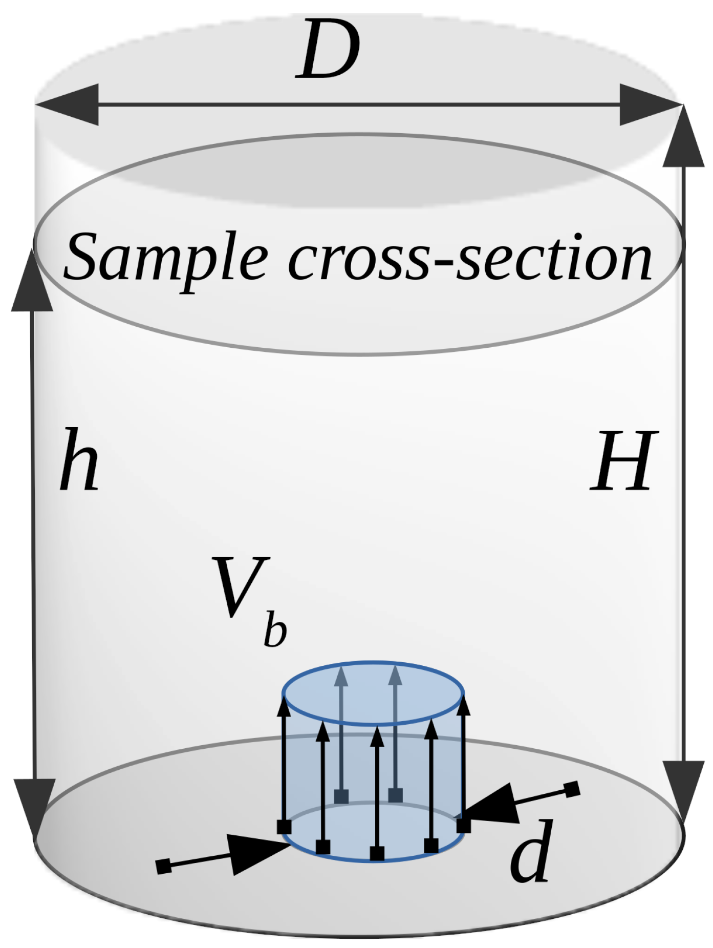
Figure 1 shows a schematic diagram of an axisymmetric BCR; reactor diameter is D = 0.07 m and reactor height is H = 0.65 m. The carrier phase is water. The disperse phase, in the form of polydisperse gas bubbles, enters the column through a coaxial axisymmetric bottom mounted aerator (d = 0.05 m).
A cross-section at a height of h = 0.48 m, depicted in the scheme, is used as a reference cross-section for the presentation of flow parameters.
Normal conditions for ambient gas at the free surface are assumed.
Simulations were carried out on a mesh of 50 cells along the radial coordinate and 90 cells along the axial coordinate, with the mesh denser toward the solid boundaries to provide detailed boundary layer resolution to meet both multiphase and turbulence requirements. Independent mesh sensitivity studies were performed and the presented mesh was selected as adequate. The time step was chosen equal to s with a normalized convergence criterion of for each independent variable.
3.2. A Discrete Approximation of the BSD Function
The initial BSD can be described by the lognormal function (2). To determine the most efficient variant of the piecewise constant approximation of this function, three sets of approximations are used, denoted by R1, R2 and R3. The entire interval of bubble size variation is replaced by the range , where , which corresponds to 99.7% of all bubbles. The R1 distribution approximation is uniform with respect to the variable in the range ; the entire range is divided into N classes, each class having the same width with respect to . The R2 distribution approximation is uniform with respect to the variable ; the range is divided into N classes, the width of each class with respect to is the same. The R3 approximation is a hybrid R2–R1: the first classes are uniformly distributed with respect to the variable in the range ; the subsequent classes are uniformly distributed with respect to the variable in the range .
The distribution approximation of type R1 is used for validation purposes. A set of different numbers of classes is used with N = [1…10], covering a range from a monodisperse approach to a detailed polydisperse one. The validation is performed for the characteristic bubble size M = 0.5 mm.
The lognormal distributions under consideration correspond to four characteristic bubble sizes M: 0.25 mm, 0.375 mm, 0.5 mm and 1.0 mm. Five combinations of the number of classes and distribution approximation options are introduced: (N = 1, R1), which corresponds to monodisperse bubbles, (N = 4, R3), which corresponds to a compact economic distribution, (N = 7, R1) and (N = 7, R2), which allow a qualitative description of the polydisperse medium, and (N = 10, R3), which provides a detailed description of the polydisperse bubble flow.
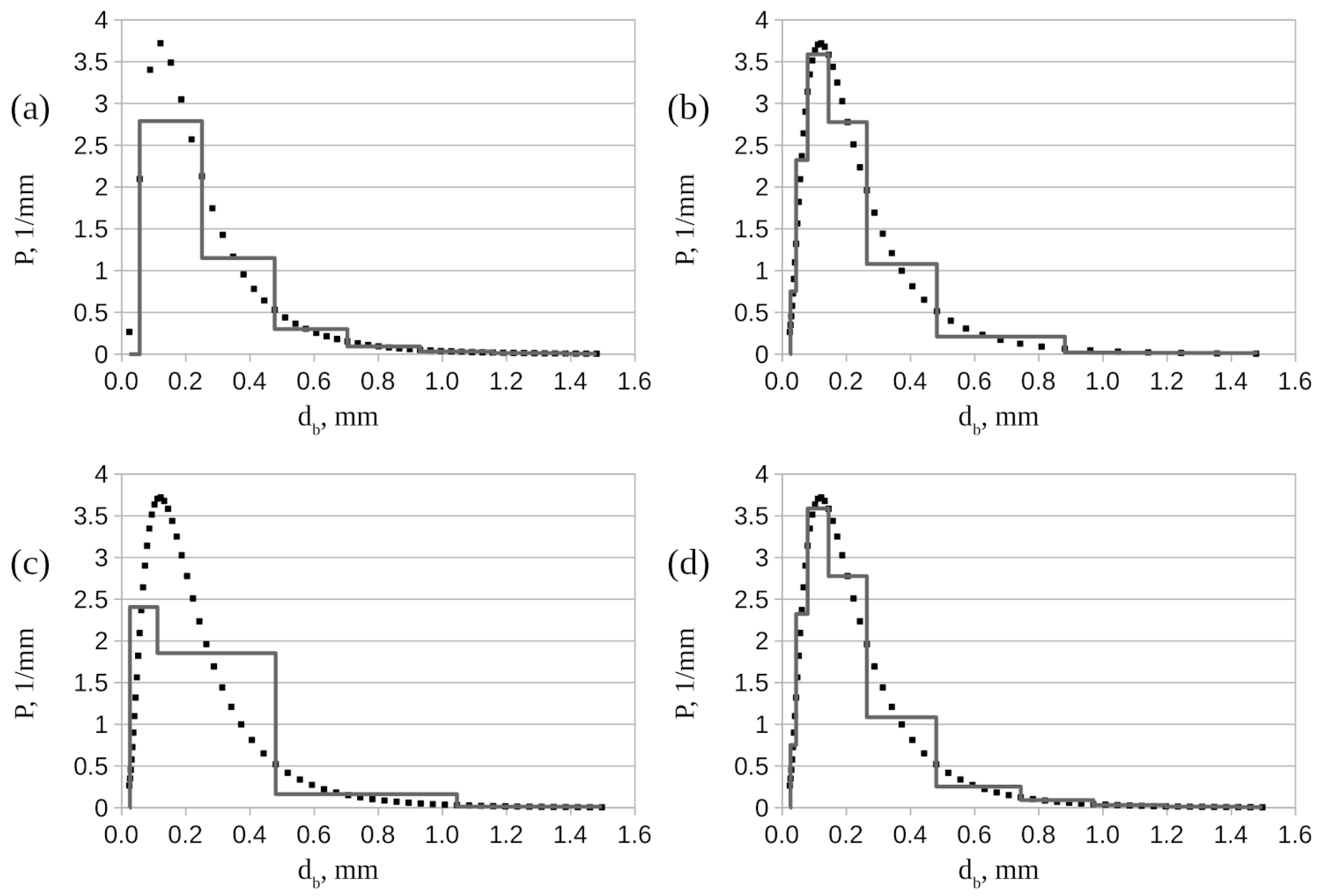
The discretized BSDs for the characteristic bubble size = 0.25 mm are shown in Figure 2, with the exception of the monodisperse one, since it is elementary. It is worth noting some features of these distributions.
It can be seen that the distribution (N = 7, R1) does not describe the features of the distribution of small bubbles, providing for this domain only one class for bubbles from 0 to 0.25 mm. The distribution (N = 7, R2) resolves small bubbles at the expense of details for large bubbles. The distribution (N = 4, R3), despite some roughness, singles out a class for small and medium bubbles. The distribution (N = 10, R3) is the most detailed, describing both small and large bubbles well over the entire range.
4. Results and Discussion
4.1. Algorithm Verification
To assess the convergence of the algorithm by the number of classes N, the following parameters are used: the interfacial area , the bubble volume fraction , the bubble velocity and the liquid velocity . The bubble volume fraction, interfacial area and bubble velocity are calculated as follows:
The overall averaged values are used to monitor the convergence to a stable solution as N increases, as well as the deviation of solutions with number of classes N and N-1.
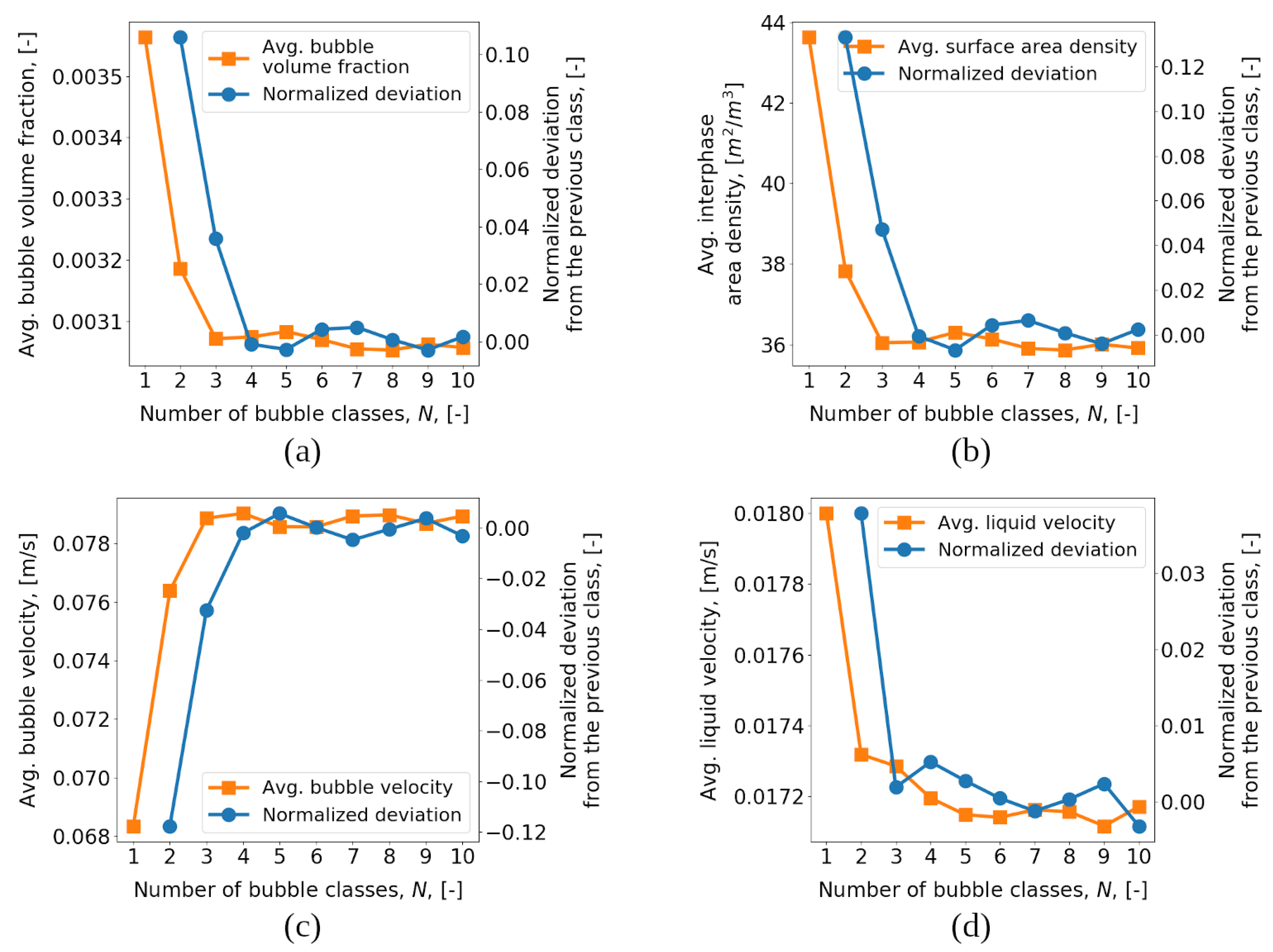
Figure 3 shows the averaged values of the variables mentioned above and the normalized deviation of the variable values compared to the solution obtained for N-1 bubble classes as a function of the number of classes. Due to the averaging procedure, these values represent the entire flow behavior. Figure 3 shows the averaged values of the above variables as a function of the number of classes and the normalized deviation of the variable values compared to the solution obtained for N-1 bubble classes. Due to the averaging procedure, the values represent the entire flow behavior.
It can be seen that the monodisperse approach overpredicts the total gas holdup within a column as well as the interfacial density. With increasing N the solution tends to converge to the polydisperse solution, with normalized deviation tending to the vicinity of zero at for the bubble volume fraction, the interfacial area density and the bubble velocity. The differences between the variants are less than 1% at N = 4, indicating that sufficient detail is captured to estimate the integral flow parameters. However, the fluid velocity, despite having the lowest normalized deviation, also has the lowest rate of deviation decay, approaching 0 at . Thus, a converged solution in terms of N can be obtained at N = 7.
4.2. An Impact of Characteristic Bubble Size and Parameters of Approximation of the BSD Function on the Flow Structure
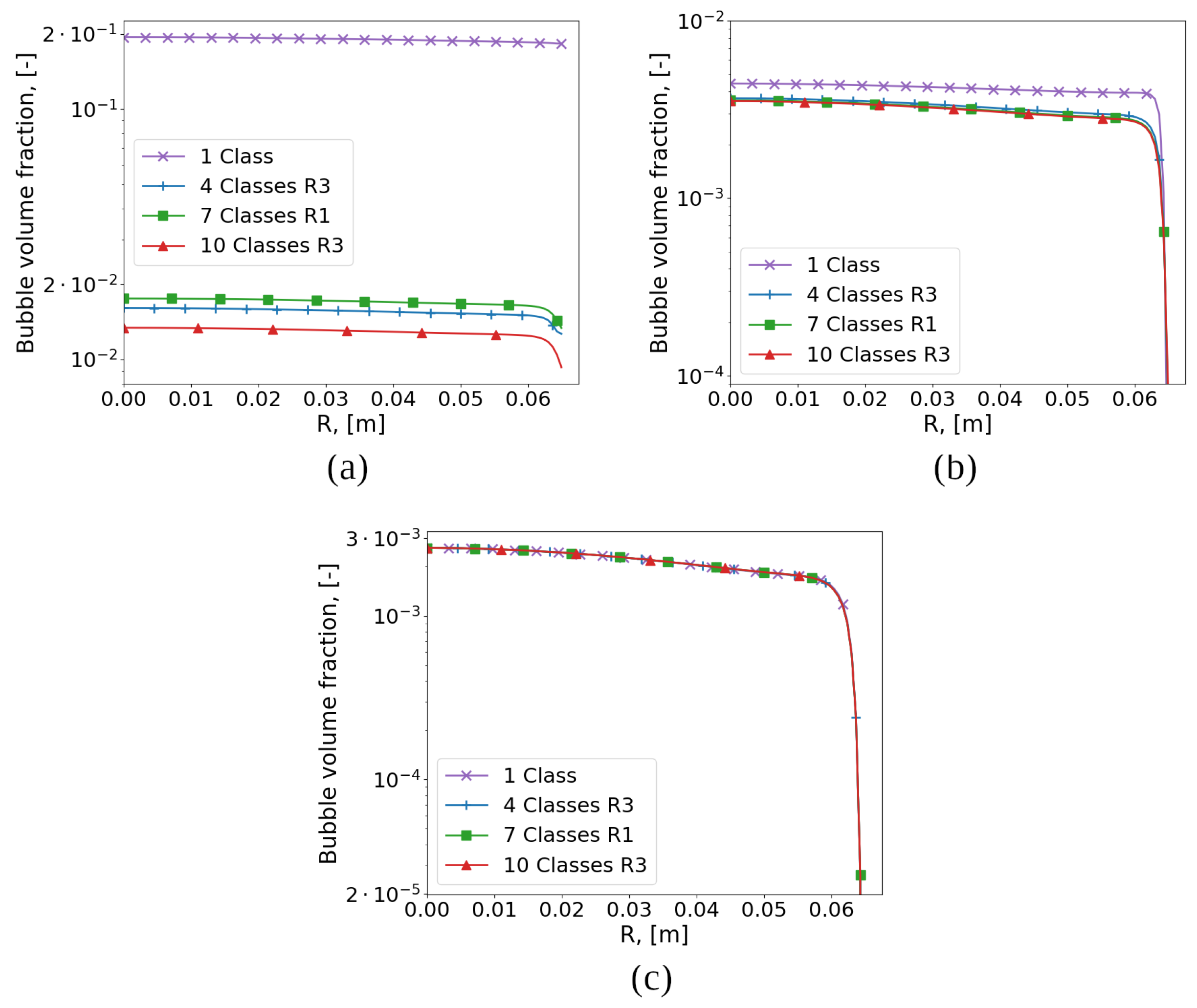
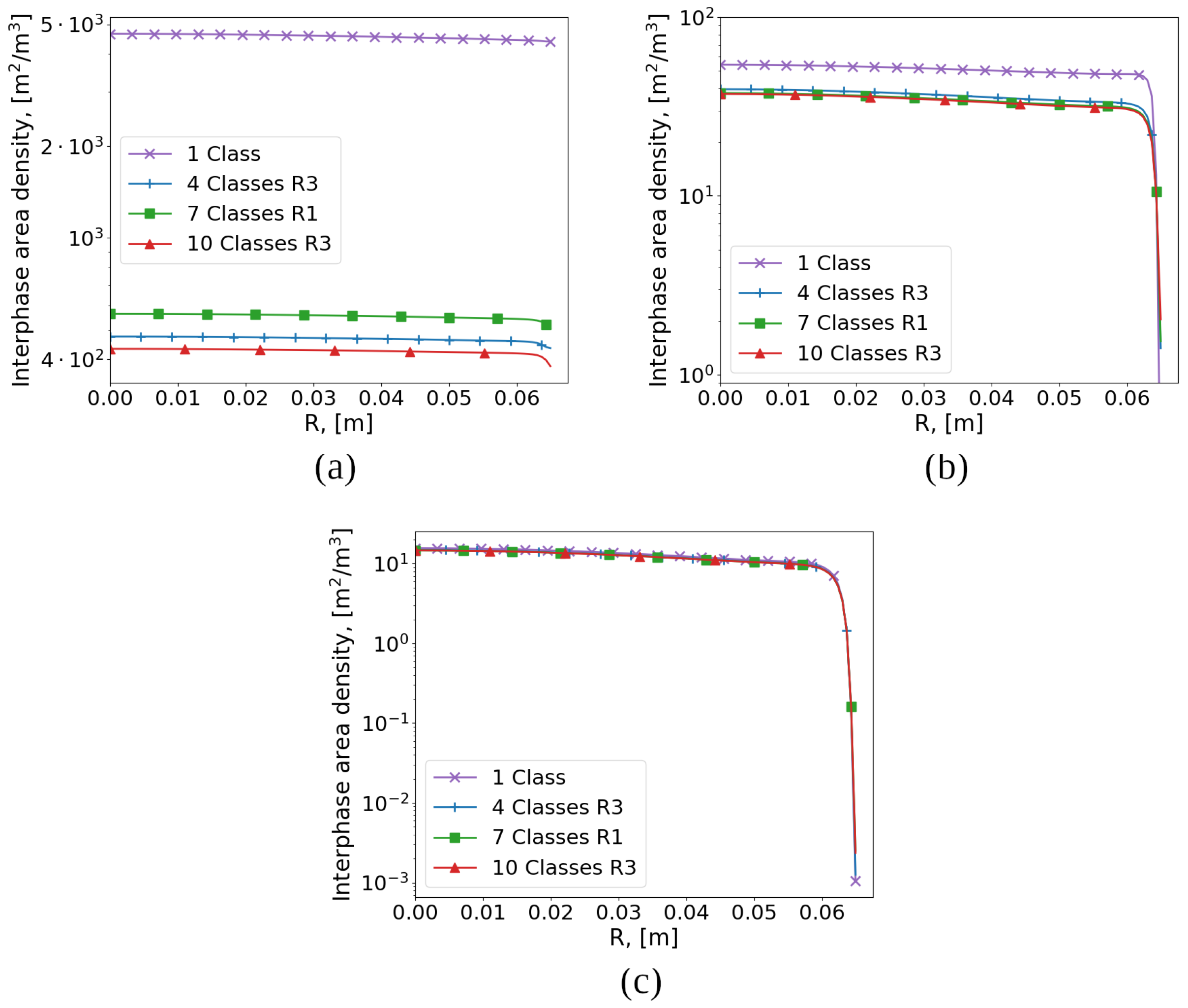
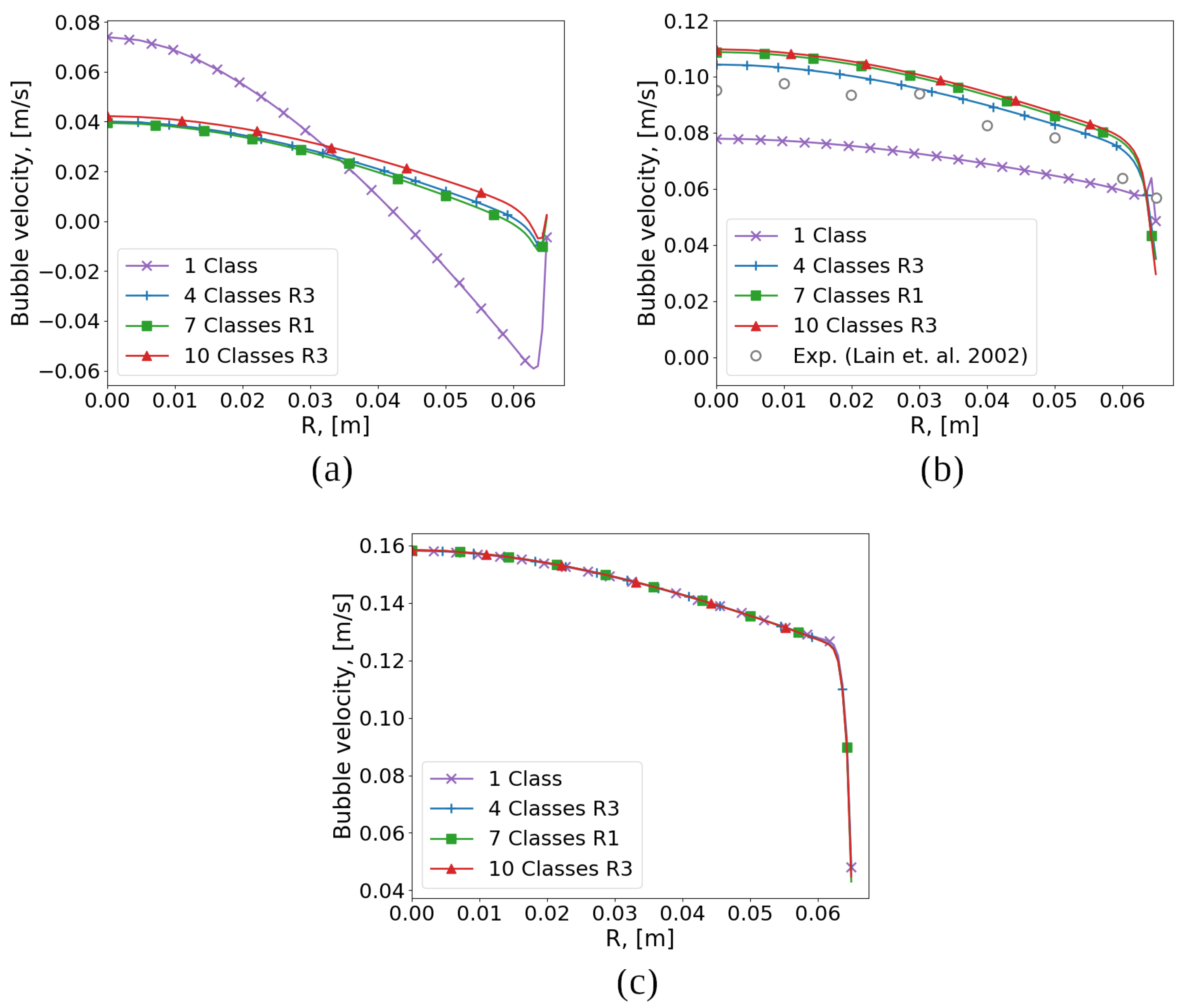
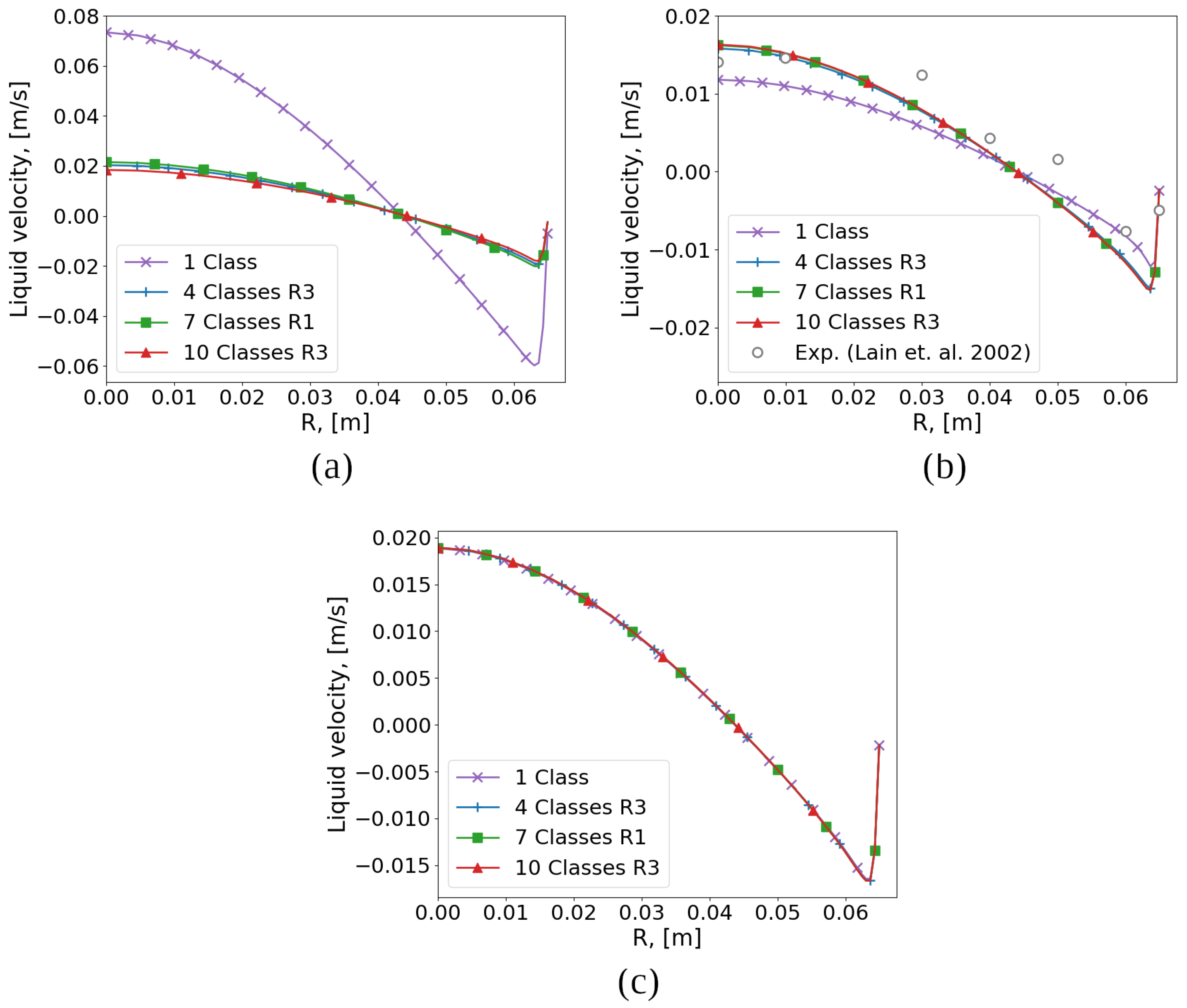
Some results of the BCR flow simulation are presented below. The radial profiles of the bubble volume fraction (Figure 4), the interfacial surface area (Figure 5), the bubble velocity (Figure 6) and the carrier phase velocity (Figure 7) are shown.
The data correspond to the reference cross-section (see Figure 1) for three characteristic bubble sizes (0.25 mm, 0.5 mm and 1 mm) and four variants of approximations: (N = 1, R1), (N = 4, R3), (N = 7, R1) and (N = 10, R3).
It can be seen that for small bubbles ( = 0.25 mm) there is a significant difference between the monodisperse and polydisperse approaches in all studied parameters. As the bubble size increases ( = 1.00 mm), the profiles of the volume fraction and the velocity of the carrier phase coincide for the two approaches. It should also be noted that, although the variant (N = 4, R3) has fewer bubble classes than (N = 7, R1), it gives a solution close to (N = 10, R3) for the volume fraction and the interfacial area, in contrast to (N = 7, R1). A comparison with the experimental data [22] for = 0.5 mm shows that the option (N = 4, R3) is preferable.
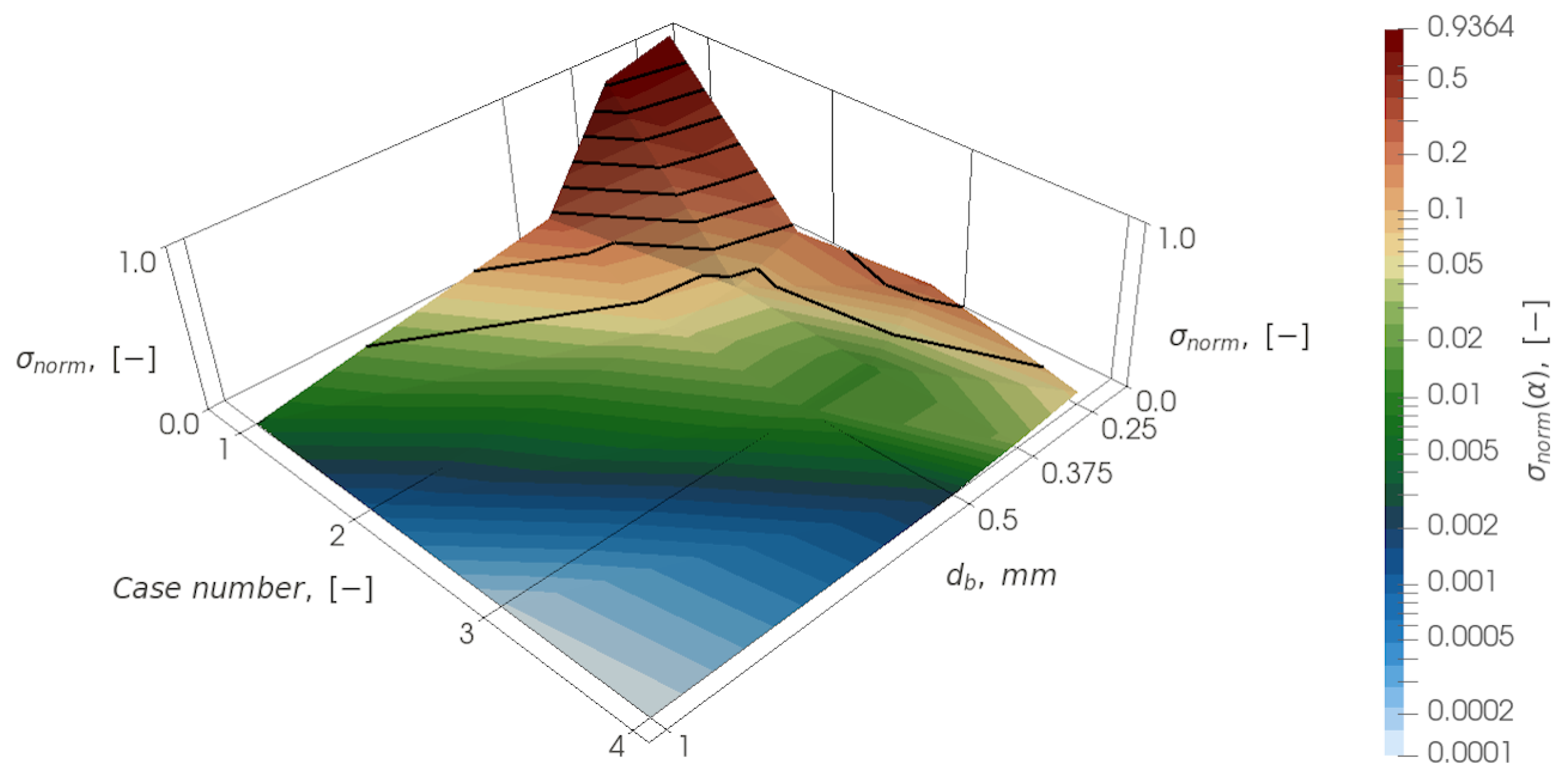
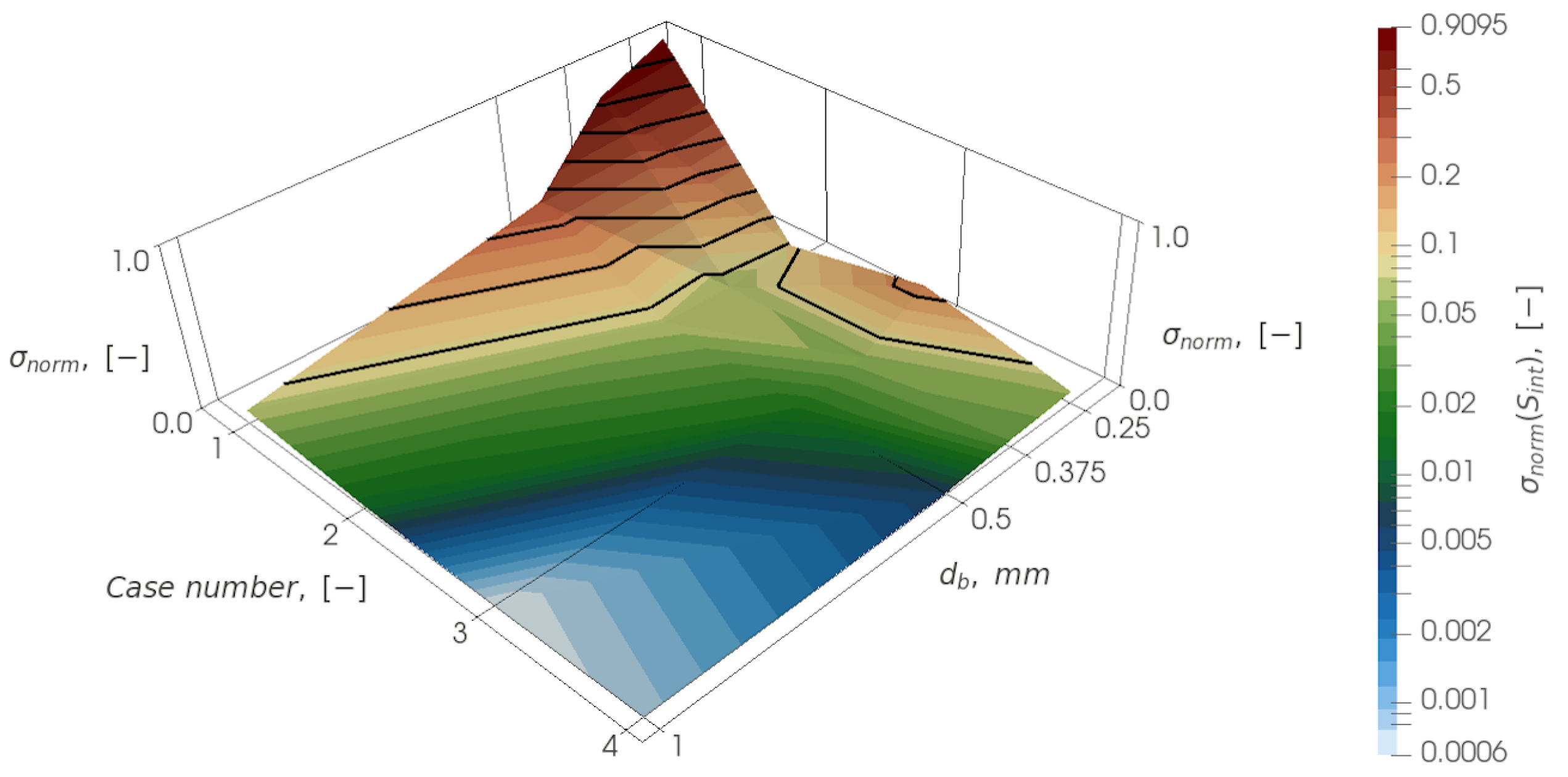
The main emphasis is placed on the comparison of the obtained solutions with the “reference” solution for the case (N = 10, R3) as the most detailed representation of the BSD function. The comparison was carried out using the normalized variance of the obtained solution and the “reference” solution in the entire domain for a set of characteristic values of the polydisperse flow, such as the velocities of the carrier and dispersed phases, the volume fraction of the bubbles, and the interfacial area. The normalized variance was estimated according to the formula:
where is the comparable variable for the solution under study and is the same variable in the same cell for the “reference” solution.
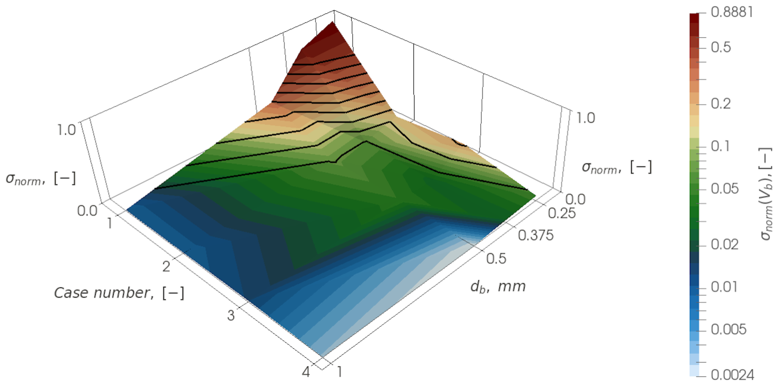
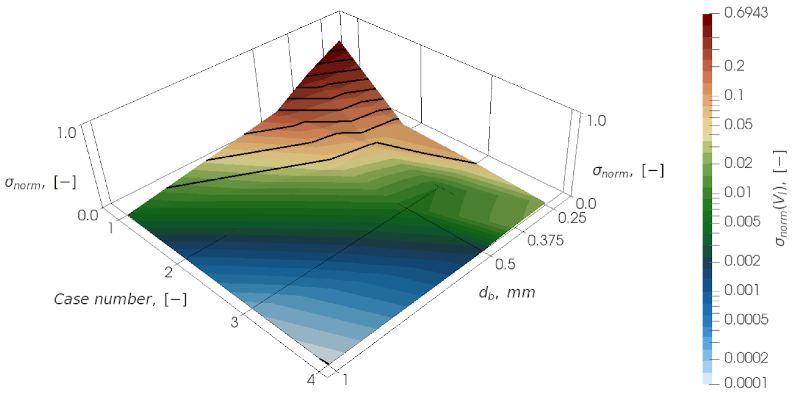
Below are plots of the weighted variances, , as a function of case number and bubble diameter, . For the case numbers, 1 stands for (N = 1, R1), 2 stands for (N = 4, R3), 3 stands for (N = 7, R1) and 4 stands for (N = 7, R2) (Figure 8, Figure 9, Figure 10 and Figure 11).
Based on the analysis of all four distributions, a general conclusion can be drawn: as the characteristic size of the bubbles increases, the difference between all approaches is leveled and, even for the monodisperse approach, the difference with the reference one turns out to be small: it is 5% for the interfacial area and about 1% for other quantities for a bubble diameter of 1 mm. However, for a bubble diameter of 0.5 mm, the difference between the monodisperse and polydisperse approaches becomes significant (up to 20%). The difference increases with decreasing bubble diameter.
For 0.5 mm bubbles the normalized variance decreases monotonically and the solution approaches the reference one with increase of N (variation of the parameters of the BSD function approximation): from monodisperse (N = 1, R1), then through distributions (N = 4, R3), (N = 7, R1) and ending with (N = 7, R2).
However, for the smallest bubble considered, with a diameter of 0.25 mm, this behavior changes. Using the distribution (N = 4, R3), a solution can be obtained that is close to the variant (N = 7, R2) and has a smaller difference from the “reference” one than (N = 7, R1). This can be explained by the fact that, in the case of the distribution (N = 7, R1), small bubbles corresponding to the left side of the BSD function are not resolved at all in the simulation. However, their influence is important since they have the ability to accumulate in stagnation or recirculation zones, significantly influencing the flow parameters and changing the flow structure. Although the distribution (N = 4, R3) is coarser than (N = 7, R1), it still describes the behavior of small bubbles.
5. Conclusions
The numerical simulation of the dynamics of polydisperse and monodisperse flows in the BCR was performed to clarify the effect of the parameters of the piecewise constant approximation of the BSD function.
It was found that with increasing of bubble size the normalized variances of the bubble volume fraction, the liquid velocity, and the specific density of the interfacial surface calculated for the polydisperse and monodisperse descriptions of the BCR working medium decrease. In particular, for bubbles with a characteristic size of M = 1.0 mm, the normalized variance is about 1% for the velocity and 5% for the density of the interfacial surface.
The discrete approximation of the BSD function with the uniform distribution of bins with respect to (R2) provides a better solution, in terms of normalized variances, than that with the uniform bins with respect to (R1), due to the correct resolution of the domain of small bubbles (with < M).
A hybrid approximation of the BSD function R3 has been proposed which is uniform with respect to for bubbles with sizes smaller than M and uniform with respect to for sizes larger than M. Such an approximation is potentially preferable with substantially large bubble sizes up to ( > 6 mm).
The hybrid approximation of the BSD (R3) with four classes of bubbles provides better results than the original R1 approximation with seven classes and is comparable to the R2 approximation with seven classes of bubbles. The obtained results were compared with the results for the R3 approximation with 10 classes of bubbles as well as with the experimental data, and demonstrated qualitative and quantitative agreement. This makes the proposed approach promising for flow pattern prediction and robust due to low computational resource requirements.
Author Contributions
Conceptualization, A.C. and A.S.; methodology, A.C. and A.S.; software, A.C.; validation, A.C. and V.C.; formal analysis, A.S.; investigation, A.S.; writing—original draft preparation, A.C., A.S. and V.C.; writing—review and editing, A.C. and A.S.; visualization, A.C. and V.C.; supervision, A.S.; project administration, A.S.; funding acquisition, A.S. All authors have read and agreed to the published version of the manuscript.
Funding
This research received no external funding.
Institutional Review Board Statement
Not applicable.
Informed Consent Statement
Not applicable.
Data Availability Statement
Data available upon request.
Conflicts of Interest
The authors declare no conflict of interest.
Abbreviations
The following abbreviations are used in this manuscript:
| BCR | Bubble column reactor |
| BSD | Bubble size distribution |
| MUSIG | Multiple size group |
| TVD | Total variation diminishing |
| SIMPLE | Semi-implicit method for pressure-linked equations |
References
- Yang, X.; Liu, Z.; Manhaeghe, D.; Yang, Y.; Hogie, J.; Demeestere, K.; van Hulle, S.W.H. Intensified ozonation in packed bubble columns for water treatment: Focus on mass transfer and humic acids removal. Chemosphere 2021, 283, 131217. [Google Scholar] [CrossRef] [PubMed]
- Inkeri, E.; Tynjälä, T. Modeling of CO2 Capture with Water Bubble Column Reactor. Energies 2020, 13, 5793. [Google Scholar] [CrossRef]
- Perez, B.J.L.; Jimenez, J.A.M.; Bhardwaj, R.; Goetheer, E.; van Sint Annaland, M.; Gallucci, F. Methane pyrolysis in a molten gallium bubble column reactor for sustainable hydrogen production: Proof of concept & techno-economic assessment. Int. J. Hydrogen Energy 2021, 46, 4917–4935. [Google Scholar] [CrossRef]
- Vik, C.B.; Solsvik, J.; Hillestad, M.; Jakobsen, H.A. Interfacial mass transfer limitations of the Fischer-Tropsch synthesis operated in a slurry bubble column reactor at industrial conditions. Chem. Eng. Sci. 2018, 192, 1138–1156. [Google Scholar] [CrossRef]
- Kantarci, N.; Borak, F.; Ulgen, K.O. Bubble column reactors. Process Biochem. 2005, 40, 2263–2283. [Google Scholar] [CrossRef]
- Lau, Y.M.; Thiruvalluvan Sujatha, K.; Gaeini, M.; Deen, N.G.; Kuipers, J.A.M. Experimental study of the bubble size distribution in a pseudo-2D bubble column. Chem. Eng. Sci. 2013, 98, 203–211. [Google Scholar] [CrossRef]
- Besagni, G.; Inzoli, F. Prediction of Bubble Size Distributions in Large-Scale Bubble Columns Using a Population Balance Model. Computations 2019, 7, 17. [Google Scholar] [CrossRef] [Green Version]
- Pakhomov, M.A.; Terekhov, V.I. Simulation of the turbulent structure of a flow and heat transfer in an ascending polydisperse bubble flow. Tech. Phys. 2015, 60, 1268–1276. [Google Scholar] [CrossRef]
- Yao, W.; Morel, C. Volumetric interfacial area prediction in upward bubbly two-phase flow. Int. J. Heat Mass Transf. 2004, 47, 307–328. [Google Scholar] [CrossRef]
- Wang, T.; Wang, J.; Jin, Y. Population Balance Model for Gas-Liquid Flows: Influence of Bubble Coalescence and Breakup Models. Ind. Eng. Chem. Res. 2005, 44, 7540–7549. [Google Scholar] [CrossRef]
- Lo, S. Application of Population Balance to CFD Modelling of Bubbly Flow via the MUSIG Model; AEA Technology: Rotherham, UK, 1996. [Google Scholar]
- Krepper, E.; Lucas, D.; Frank, T.; Prasser, H.-M.; Zwart, P.J. The inhomogeneous MUSIG model for the simulation of polydispersed flows. Nucl. Eng. Des. 2008, 238, 1690–1702. [Google Scholar] [CrossRef]
- Ziegenhein, T.; Rzehak, R.; Lucas, D. Transient simulation for large scale flow in bubble columns. Chem. Eng. Sci. 2015, 122, 1–13. [Google Scholar] [CrossRef]
- Olmos, E.; Gentric, C.; Vial, C.; Wild, G.; Midoux, N. Numerical simulation of multiphase flow in bubble column reactors. Influence of bubble coalescence and break-up. Chem. Eng. Sci. 2001, 56, 6359–6365. [Google Scholar] [CrossRef]
- Fard, M.G.; Stiriba, Y.; Gourich, B.; Vial, C.; Grau, F.X. Euler–Euler large eddy simulations of the gas–liquid flow in a cylindrical bubble column. Nucl. Eng. Des. 2020, 369, 110823. [Google Scholar] [CrossRef]
- Zhang, X.B.; Yan, W.C.; Luo, Z.H. Numerical simulation of local bubble size distribution in bubble columns operated at heterogeneous regime. Chem. Eng. Sci. 2021, 231, 116266. [Google Scholar] [CrossRef]
- Wu, Y.; Liu, Z.; Li, B.; Gan, Y. Numerical simulation of multi-size bubbly flow in a continuous casting mold using population balance model. Powder Technol. 2022, 396, 224–240. [Google Scholar] [CrossRef]
- Wu, Y.; Liu, Z.; Li, B.; Xiao, L.; Gan, Y. Numerical simulation of multi-size bubbly flow in a continuous casting mold using an inhomogeneous multiple size group model. Powder Technol. 2022, 402, 117368. [Google Scholar] [CrossRef]
- Bhole, M.R.; Joshi, J.B.; Ramkrishna, D. CFD simulation of bubble columns incorporating population balance modeling. Chem. Eng. Sci. 2008, 63, 2267–2282. [Google Scholar] [CrossRef]
- Chernyshev, A.S.; Schmidt, A.A. Investigation of the evolution of the bubble size distribution in the ascending and descending flows. J. Phys. Conf. Ser. 2017, 899, 032009. [Google Scholar] [CrossRef] [Green Version]
- Lain, S.; Broder, D.; Sommerfeld, M. Experimental and numerical studies of the hydrodynamics in a bubble column. Chem. Eng. Sci. 1999, 54, 4913–4920. [Google Scholar] [CrossRef]
- Lain, S.; Broder, D.; Sommerfeld, M.; Goz, M.F. Modelling hydrodynamics and turbulence in a bubble column using the Euler–Lagrange procedure. Int. J. Multiph. Flow 2002, 28, 1381–1407. [Google Scholar] [CrossRef]
- Roghair, I.; Lau, Y.M.; Deen, N.G.; Slagter, H.M.; Baltussen, M.W.; van Sint Annaland, M.; Kuipers, J.A.M. On the drag force of bubbles in bubble swarms at intermediate and high Reynolds numbers. Chem. Eng. Sci. 2011, 66, 3204–3211. [Google Scholar] [CrossRef]
- Auton, T.R. The lift force on a spherical body in a rotational flow. J. Fluid Mech. 1987, 183, 199–218. [Google Scholar] [CrossRef]
- Tomiyama, A.; Tamai, H.; Zun, I.; Hosokawa, S. Transverse migration of single bubbles in simple shear flows. Chem. Eng. Sci. 2002, 57, 1849–1858. [Google Scholar] [CrossRef]
- Menter, F.R.; Kuntz, M.; Langtry, R. Ten Year of Industrial Experience with the SST Turbulence Model. In Proceedings of the 4th International Symposium on Turbulence, Heat and Mass Transfer, Antalya, Turkey, 12–17 October 2003; pp. 625–632. [Google Scholar]
- Troshko, A.A.; Hassan, Y.A. A two-equation turbulence model of turbulent bubbly flows. Int. J. Multiph. Flow 2001, 27, 1965–2000. [Google Scholar] [CrossRef]
- Sato, Y.; Sekoguchi, R. Liquid velocity distribution in two-phase bubble flow. Int. J. Multiph. Flow 1975, 2, 79–95. [Google Scholar] [CrossRef]
- Sokolichin, A.; Eigenberger, G.; Lapin, A. Simulation of Buoyancy Driven Bubbly Flow: Established Simplifications and Open Questions. AIChE J. 2004, 50, 24–45. [Google Scholar] [CrossRef]
- Moraga, F.J.; Larreteguy, A.E.; Drew, D.A.; Lahey, R.T., Jr. Assessment of turbulent dispersion models for bubbly flows in the low Stokes number limit. Int. J. Multiph. Flow 2003, 29, 655–673. [Google Scholar] [CrossRef]
- Versteeg, H.K.; Malalasekera, W. An Introduction to Computational Fluid Dynamics. The Finite Volume Method, 2nd ed.; Pearson Education Limited: Harlow, UK, 2007; pp. 134–211. [Google Scholar]
- Chernyshev, A.S.; Schmidt, A.A. Numerical modeling of gravity-driven bubble flows with account of polydispersion. J. Phys. Conf. Ser. 2016, 754, 032005. [Google Scholar] [CrossRef] [Green Version]
- Chernyshev, A.S.; Schmidt, A.A. Numerical simulation of gravity-driven mono- and polydisperse bubbly flows in a three-dimensional column in the framework of the Euler–Euler approach. J. Phys. Conf. Ser. 2020, 1697, 012236. [Google Scholar] [CrossRef]
- Chen, P.; Sanyal, J.; Dudukovic, M.P. Numerical simulation of bubble columns flows: Effect of different breakup and coalescence closures. Chem. Eng. Sci. 2005, 60, 1085–1101. [Google Scholar] [CrossRef]
- Allio, A.; Buffo, A.; Marchisio, D.; Savoldi, L. Two-fluid modelling for poly-disperse bubbly flows in vertical pipes: Analysis of the impact of geometrical parameters and heat transfer. Nucl. Eng. Technol. 2022, in press. [Google Scholar] [CrossRef]
Figure 1.
Schematics of a bubble column reactor.

Figure 2.
BSD function and piecewise approximations. The characteristic bubble size is = 0.25 mm. (a) N = 7, R1; (b) N = 7, R2; (c) N = 4, R3; (d) N = 10, R3.
Figure 2.
BSD function and piecewise approximations. The characteristic bubble size is = 0.25 mm. (a) N = 7, R1; (b) N = 7, R2; (c) N = 4, R3; (d) N = 10, R3.

Figure 3.
Distributions of flow parameters as a function of the number of bubble classes. The characteristic bubble size = 0.25 mm; (a) the bubble volume fraction; (b) the interfacial area density; (c) the bubble velocity; (d) the liquid velocity.
Figure 3.
Distributions of flow parameters as a function of the number of bubble classes. The characteristic bubble size = 0.25 mm; (a) the bubble volume fraction; (b) the interfacial area density; (c) the bubble velocity; (d) the liquid velocity.

Figure 4.
Radial profiles of the bubble volume fraction in the reference cross-section (see Figure 1) per different characteristic bubble sizes: (a) M = 0.25 mm; (b) M = 0.5 mm; (c) M = 1.0 mm.
Figure 4.
Radial profiles of the bubble volume fraction in the reference cross-section (see Figure 1) per different characteristic bubble sizes: (a) M = 0.25 mm; (b) M = 0.5 mm; (c) M = 1.0 mm.

Figure 5.
Radial profiles of the interfacial area density in the reference cross-section (see Figure 1) for different characteristic bubble sizes: (a) M = 0.25 mm; (b) M = 0.5 mm; (c) M = 1.0 mm.
Figure 5.
Radial profiles of the interfacial area density in the reference cross-section (see Figure 1) for different characteristic bubble sizes: (a) M = 0.25 mm; (b) M = 0.5 mm; (c) M = 1.0 mm.

Figure 6.
Radial profiles of bubble velocity in the reference cross-section (see Figure 1) for different characteristic bubble sizes: (a) M = 0.25 mm; (b) M = 0.5 mm; (c) M = 1.0 mm.
Figure 6.
Radial profiles of bubble velocity in the reference cross-section (see Figure 1) for different characteristic bubble sizes: (a) M = 0.25 mm; (b) M = 0.5 mm; (c) M = 1.0 mm.

Figure 7.
Radial profiles of liquid velocity in the reference cross-section (see Figure 1) for different characteristic bubble sizes: (a) M = 0.25 mm; (b) M = 0.5 mm; (c) M = 1.0 mm.
Figure 7.
Radial profiles of liquid velocity in the reference cross-section (see Figure 1) for different characteristic bubble sizes: (a) M = 0.25 mm; (b) M = 0.5 mm; (c) M = 1.0 mm.

Figure 8.
Distribution of a weighted variance for the bubble volume fraction, .

Figure 9.
Distribution of a weighted variance for the interfacial area density, .

Figure 10.
Distribution of a weighted variance for the bubble velocity, .

Figure 11.
Distribution of a weighted variance for the liquid velocity, .

Disclaimer/Publisher’s Note: The statements, opinions and data contained in all publications are solely those of the individual author(s) and contributor(s) and not of MDPI and/or the editor(s). MDPI and/or the editor(s) disclaim responsibility for any injury to people or property resulting from any ideas, methods, instructions or products referred to in the content. |
© 2023 by the authors. Licensee MDPI, Basel, Switzerland. This article is an open access article distributed under the terms and conditions of the Creative Commons Attribution (CC BY) license (https://creativecommons.org/licenses/by/4.0/).
Share and Cite
MDPI and ACS Style
Chernyshev, A.; Schmidt, A.; Chernysheva, V. An Impact of the Discrete Representation of the Bubble Size Distribution Function on the Flow Structure in a Bubble Column Reactor. Water 2023, 15, 778. https://doi.org/10.3390/w15040778
AMA Style
Chernyshev A, Schmidt A, Chernysheva V. An Impact of the Discrete Representation of the Bubble Size Distribution Function on the Flow Structure in a Bubble Column Reactor. Water. 2023; 15(4):778. https://doi.org/10.3390/w15040778
Chicago/Turabian StyleChernyshev, Alexander, Alexander Schmidt, and Veronica Chernysheva. 2023. "An Impact of the Discrete Representation of the Bubble Size Distribution Function on the Flow Structure in a Bubble Column Reactor" Water 15, no. 4: 778. https://doi.org/10.3390/w15040778
Note that from the first issue of 2016, this journal uses article numbers instead of page numbers. See further details here.