

Comparison of Three Imputation Methods for Groundwater Level Timeseries
by
 ,
,
Mara Meggiorin
1,2,*,†,
Giulia Passadore
2,
Silvia Bertoldo
1,
Andrea Sottani
1 and
Andrea Rinaldo
2,3 1
Sinergeo srl, 36100 Vicenza, Italy
2
Dipartimento di Ingegneria Civile, Edile e Ambientale, Università di Padova, 35100 Padua, Italy
3
Laboratory of Echohydrology (ECHO/IIE/ENAC), École Polytechnique Fédérale de Lausanne, 1015 Lausanne, Switzerland
*
Author to whom correspondence should be addressed.
†
Current address: Ramboll, 20159 Milan, Italy.
Water 2023, 15(4), 801; https://doi.org/10.3390/w15040801
Submission received: 27 December 2022
/
Revised: 8 February 2023
/
Accepted: 15 February 2023
/
Published: 17 February 2023
(This article belongs to the Special Issue Data-Driven Approach Supporting Groundwater Resource Understanding, Protection and Management)
Abstract
:This study compares three imputation methods applied to the field observations of hydraulic head in subsurface hydrology. Hydrogeological studies that analyze the timeseries of groundwater elevations often face issues with missing data that may mislead both the interpretation of the relevant processes and the accuracy of the analyses. The imputation methods adopted for this comparative study are relatively simple to be implemented and thus are easily applicable to large datasets. They are: (i) the spline interpolation, (ii) the autoregressive linear model, and (iii) the patched kriging. The average of their results is also analyzed. By artificially generating gaps in timeseries, the results of the various imputation methods are tested. The spline interpolation is shown to be the poorest performing one. The patched kriging method usually proves to be the best option, exploiting the spatial correlations of the groundwater elevations, even though spurious trends due to the the activation of neighboring sensors at times affect their reconstructions. The autoregressive linear model proves to be a reasonable choice; however, it lacks hydrogeological controls. The ensemble average of all methods is a reasonable compromise. Additionally, by interpolating a large dataset of 53 timeseries observing the variabilities of statistical measures, the study finds that the specific choice of the imputation method only marginally affects the overarching statistics.
1. Introduction
In the last few decades, the groundwater resource has been recognized worldwide as a critical water security player. However, increased exploitation and often the consequences of climatic change are a matter of concern [1,2]. Groundwater resources currently play an essential role in sustaining ecosystems and human activities, and the importance of sustainably managing them is broadly acknowledged [3,4,5]. Nevertheless, conflicting uses and the intrinsic complexity in measuring comprehensive groundwater systems concerts difficult assessments of the quantity and quality of the resource [6].
Hydrogeological studies often focus on the monitoring data of the groundwater piezometric head in various horizons in space and time (say, the hydraulic head), via instantaneous observations or by observing the groundwater system’s seasonality. Longitudinal observations of the hydraulic head along transects are often the starting points of studies on storages and fluxes, and they provide relevant information on the aquifers of interest [7]. Hydrogeological studies that analyze the longitudinal observations of the hydraulic head are often employed to refine the conceptual model of the system, e.g., [8,9,10], and in particular if impacts of different stressors are sought (say, shifting rainfall and increased pumping). Timeseries measurements and analyses prove to be particularly meaningful, e.g., [11,12], especially in assessing the sustainability of the withdrawals, e.g., [13,14,15,16]. They are also valuable in calibrating and validating numerical models that are focused on regional or field-scales, e.g., [17,18,19,20,21].
In this domain, optimizing monitoring networks is a challenge, e.g., [22,23,24]. The optimal management of the water resources is likewise demanding, e.g., [25,26,27,28]. Within hydrogeology, the analysis of observed timeseries of groundwater levels is commonplace, and also for different purposes: for example, to study the stress state of the source aquifer before and after large earthquakes [29], or in studies of the poroelastic subsidence in river delta domains [30]. The impacts of urban planning on prospective subsurface resources may also be tackled in this framework [31,32].
In conducting timeseries analyses, one of the major problems that are encountered by hydrogeologists lies in the degree of the completeness of the data, i.e., in the observed series lacking continuity, for whatever reason. Potentially, extended gaps may impair an overall understanding of the underlying processes and the accuracy of the analysis [33]. Missing data can be due to field issues that are encountered during monitoring campaigns based on manual measures, or malfunctioning sensors, in the case of the continuous monitoring of the groundwater level. In the latter case, typical causes of the fragmented record are faulty sensors that can remain unnoticed for a long time. In addition, groundwater levels may drop below the sensor elevation for relatively long periods of time at precisely when the data would be crucial. If gaps are few and short-lived, for standard hydrogeology purposes, the missing data may be managed with simple imputation methods. Otherwise, when the loss of information about the groundwater system might cloud important processes, this prevents proper analysis and understanding. Depending on the goal that groundwater level timeseries are used for, carefully filling of gaps could be essential, even for the shortest and most fragmented series.
Several data analyses or mathematical models require a complete dataset assuming a complete data matrix [33]. As summarized by [34], two approaches can be applied to deal with incomplete available datasets: the conservative approach that defines the minimum timeseries length and discards shorter records, possibly losing important information; and the approach that identifies alternative methodologies to gather additional information concerning the shorter series. Imputation methods for short or fragmented timeseries fall into the latter approach.
The treatment of missing values has been studied in other fields, e.g., financial economics and surface hydrology. Only a few studies have dealt specifically with the suitable interpolation applied to the groundwater level timeseries, where the issue of the proper treatment of vital missing data via automatic approaches is central. The latter are essential when using and analyzing big databases, e.g., [35]. The simplest imputation methods delete missing values or substitute the missing values with the timeseries mean. They return the complete timeseries, yet they unavoidably lose information. Thus, adding missing data with insight via more sophisticated methods is recommended [36]. By increasing the complexity of the imputation methods, other approaches deal with interpolation (e.g., linear and spline interpolations), regressions (e.g., autoregressive models by [35] or [37], artificial neural networks [38,39,40], spectral analyses [36]), or combined methods [41,42]. Such methods, however, are not optimal for the groundwater data because they often require a priori knowledge of behaviors and periodicities, which are rarely available. For spatiotemporal datasets, combining geostatistics and vector regression for infilling the missing groundwater level data is an option [43], as they do take correlations among sites into account. Another option is the least squares method to fit empirical orthogonal functions [44], but this approach needs a priori information for the spatiotemporal covariance. Recently, machine learning methods have been developed for spatiotemporal imputation, e.g., multi-layer perceptron (MLP); SOM, k-nearest neighbor (KNN); random forests, e.g., [45]; and hybrid models, e.g., [46,47]. These methods still base their results on significant hydrogeological assumptions. For example, Ref. [45] assumes that the aquifer is homogenous, and that only gradual transitions are admissible. Among these methods, a few are simple and fast to apply, but they are unrelated to the groundwater dynamics. Others are more sophisticated, but they are often based on strong assumptions, or else they are computationally demanding. Typically, therefore, they prove unsuitable for large scale applications [48].
The present comparative study aims to help field groundwater practitioners who need to choose the proper imputation method for their purposes and data, by focusing on imputation methods for groundwater level records that are relatively simple to implement in an automatic structure and that are therefore easy to use for large datasets. The forecasting methods available in Pastas [11] have not been here applied, because they require the timeseries of hydraulic drivers (e.g., rain or recharge). This feature limits their applicability for large datasets monitoring groundwater levels at regional scales. With typical field applications in mind, this study compares the three imputation methods:
- Spline interpolation (mathematical approach), which smoothly interpolates the groundwater trends;
- The autoregressive linear model (statistical approach), based on random processes where imputed values can be identified by linearly combining values previously observed;
- Patched kriging (geostatistical approach), the sequential application of the ordinary kriging, preserving the available spatio-temporal information [34].
Moreover, the ensemble average of the results obtained using the three imputation methods is also considered, and is compared with the others. These methods are implemented in this study as a first attempt for hydrogeological timeseries interpolation, and for a comparison of their statistical results. Thus, assumptions and simplifications have been here applied that can be modified and improved.
The goal is to rank methodologies for the imputation of field subsurface hydraulic head data. The comparison is carried out using two different procedures. The former compares three long timeseries by artificially creating missing values in the available records, to check a posteriori which method best reproduces the actual timeseries in the time domain. Relevant statistics of the source and reconstructed timeseries are also explored. The latter instead proposes a comparison based on whole datasets, i.e., by applying the same statistical analyses to the whole available dataset where gaps are present and where real timeseries are unknown. This procedure is useful for testing different interpolation results on real records. The main results concern the strengths and weaknesses of the various approaches, with recommendations for practical use in cases of common field relevance.
2. Materials and Methods
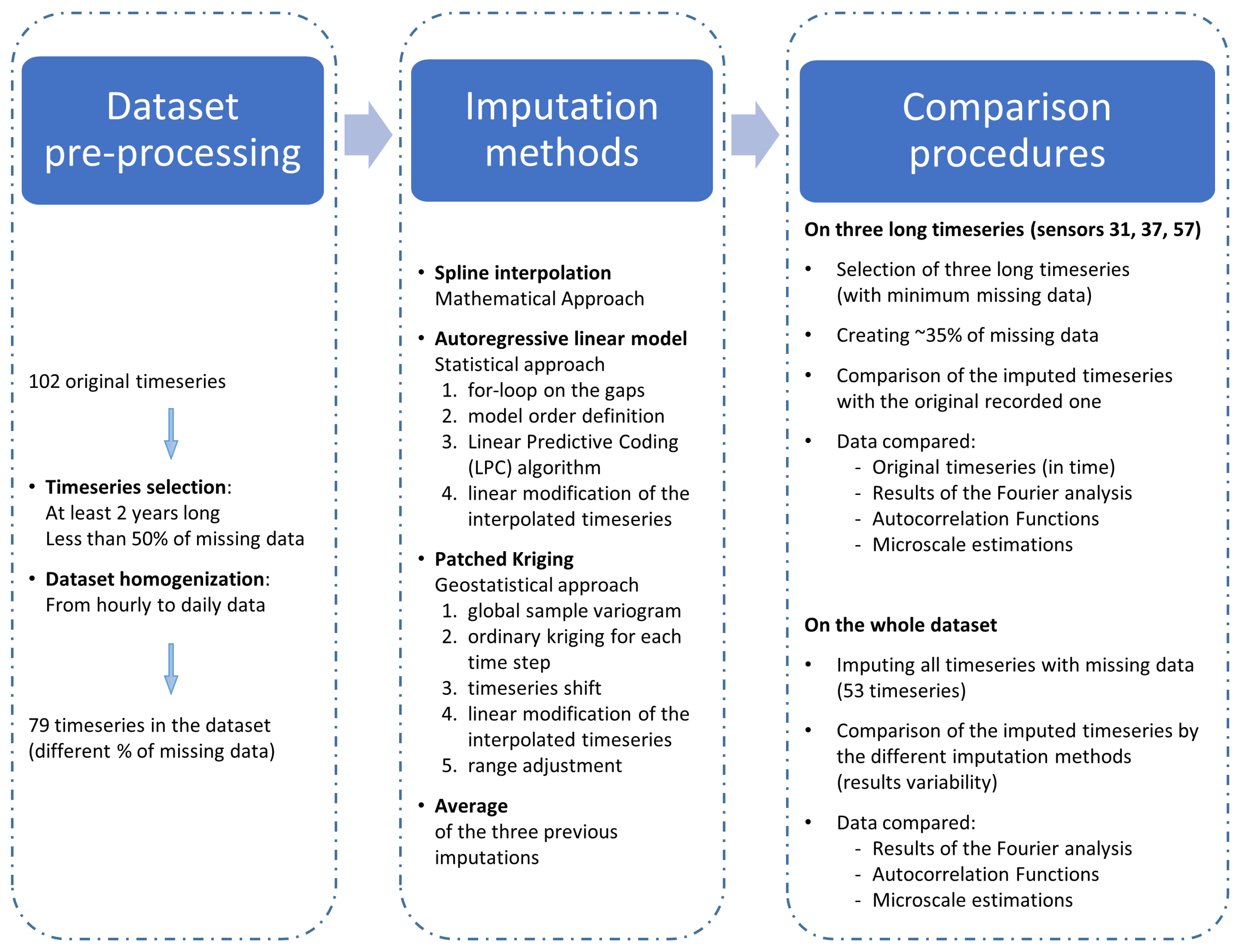
First, this section briefly presents the study area, the available dataset, and how it has been pre-processed for the following analyses, i.e., timeseries selection and dataset homogenization. Second, the selected imputation methods are briefly described, with particular focus on the description of groundwater-specific corrections. Finally, two different procedures are applied to compare the imputation methods based on the results of three statistical analyses, namely: Fourier analysis, the study of autocorrelation functions, and the evaluation of microscales (the time interval over which the signal may be assumed to be perfectly correlated). The two comparison procedures have a slightly different objective: (i) a comparison of the interpolated timeseries with the original recorded timeseries, and (ii) an analysis of the results’ variability, depending on the applied imputation method. A flowchart of the analysis is shown in Figure 1.
2.1. Overview of the Study Area
The study area where the monitoring network is located covers most of the Bacchiglione river basin (Veneto, Italy) within the alluvial plain north of the city of Vicenza. Overall, the hydrologic domain comprises approximately km. It is confined by the Asiago plateau and the Tretto area at the northern boundary, and by the Lessini mountain range westwards. The study area corresponds to the domain of earlier subsurface hydrology studies [10,16]. Several waterways drain the area in the NW–SE direction, then discharging into the Adriatic sea. The area is characterized by Quaternary deposits lying on a bedrock whose depth ranges between a few meters in the upper plain to several hundred meters towards the southeast. In the upper plain, the subsoil is mainly course material and the aquifer is undifferentiated, while towards the lower plain coarse layers vanish and a clearly stratified structure (hosting up to six clearly differentiated aquifers) appears [49,50]. The study area thus includes a hydrogeological system comprising both a large unconfined aquifer where the water table oscillates following the vagaries of hydrologic recharge; and (ii) a layered confined multi-aquifer system that is highly valuable for its protection from surface pollution [16].
2.2. Dataset Pre-Processing
The imputation methods have been applied to a proprietary dataset, collected and made available by Sinergeo srl, which has an extensive monitoring network recording the groundwater level within the study area. The proprietary dataset used for the comparison of imputation methods corresponds to the one used and presented in [16], where a detailed table reports the specifics of the monitoring network (e.g., the recorded period and the percentages of missing values for each timeseries). Briefly, the groundwater levels are monitored in 102 locations, with a sampling interval of 1 or 3 h. The available timeseries have different overall durations, ranging from 3 months to almost 14 years. Moreover, as for many real case studies, the dataset is affected by missing values and outliers. A series selection has been carried out to have at least 2 years of data per series, and less than of missing values after the outliers had been removed. As a result, the final dataset includes 79 series (Figure 2). Furthermore, in order to homogenize the dataset, hourly records have been suitably transformed into daily data.
2.3. Imputation Methods
The study applied three existing imputation methods, described in this section, adapted to the treatment of groundwater level timeseries. The first two, namely the cubic spline interpolation and the autoregressive linear model, focus on a single timeseries, while the patched kriging exploits the spatial correlation structure shown by the measured groundwater levels. Thus, the applied methods test the applicability, and the quality of the resulting fit, of both time and spatial imputation. In order to describe and to better comprehend the adjustments needed to the selected imputation methods, the resulting interpolated timeseries are reported and commented for three complete long samples (sensors 31, 37, and 57, shown in Figure 2). The same timeseries were used for comparative purposes when gaps were artificially created by removing recorded data.
The cubic spline interpolation (CS) is a mathematical interpolation, which, based on the information of the timeseries alone, applies a piecewise cubic polynomial approximating function to obtain a smooth approximation. As explained by [51], the piecewise cubic interpolators f handle data points with . In each subinterval , the interpolating function f coincides with a polynomial of order 4 that satisfies the following conditions:
where are defined as “free slopes”. Therefore, the interpolating f agrees with the data points, it is continuous, and it has a continuous first derivative on the interval . There exist different piecewise interpolation schemes, depending on the choice of the slopes evaluation: the applied CS interpolation adds the condition where the second derivative of the interpolating function f is also continuous; thus, f is twice continuously differentiable: . In this analysis, the interpolation is carried out by calling the spline function in MATLAB.
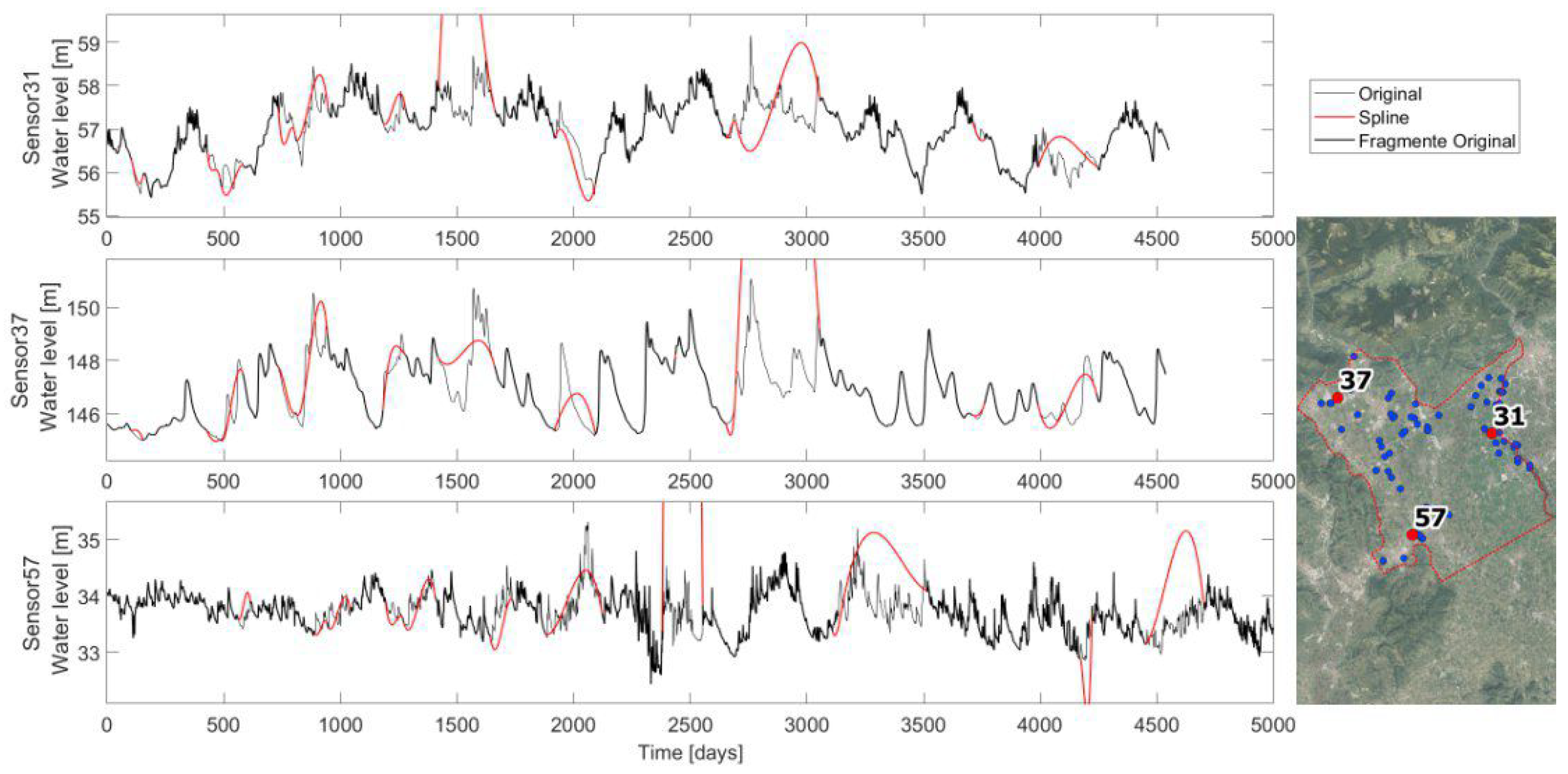
The resulting CS interpolations for sensors 31, 37, and 57 are reported in Figure 3. As is noticeable, sometimes the spline interpolation achieves maximums and minimums that are never observed by the recorded timeseries. If this happens, the CS is not considered as a plausible imputation method. The exact applied conditions are:
- The minimum spline value must be greater than the recorded minimum less one quarter of the recorded range;
- The maximum spline value must be smaller than the recorded maximum plus one quarter of the recorded range.
The autoregressive linear model (AR) is a statistical approach which, based on the information of the timeseries alone, aims to predict a realization of an underlying random processes based on past observations. Specifically, the estimated present value at k is considered to be approximated by a linear combination of n past observations. The number of past values n used by the procedure is the model order, and it intends to represent the process memory. The coefficients selected for the linear combination are constant parameters of the model that are therefore considered to be invariant in time.
In order to apply an AR model to a timeseries, it is required to first identify the appropriate order, and to estimate the coefficients by using the Linear Predictive Coding (LPC) algorithm—lpc function in MATLAB. In this study, the code used is the one described by [35], which has been adapted to this specific groundwater analysis. The code’s specifications are in [52]. What follows outlines the general procedure and the changes that are implemented. The basic assumptions are also discussed.
The AR procedure starts from a simple linear interpolation of all intervals of missing values shorter than 5 days and from a for-loop on the remaining gaps in the timeseries. For each gap, the model order is assumed to be equal to three-quarters of the prior known record length in order to use most of the available information. The known sequence is subtracted by its own mean, and the coefficients are estimated with the LPC algorithm, considering the modified timeseries. The forecast series imputing the gap is estimated using the identified linear combination, and by adding again the previously subtracted mean. Sometimes, the AR forecasted series ends () with a value that considerably diverges from the first known value after the gap , thus creating an unrealistic step-shaped trend. This happens as this forecasting procedure does not consider the available knowledge of the recorded sequence after the gap. In order to adjust such a final step, the interpolated timeseries is linearly modified within the gap in order to obtain a final forecasted value coinciding with the first value of the following known record: i.e., the timeseries S is corrected by summing up a linearly increasing factor that ranges from 0 in the first unknown value (), and in the last unknown value (). The timeseries is then updated with the interpolated sequence and the following gap of the for-loop will consider all previous values as being known and usable for its own interpolation. This for-loop applies only if the previous knowledge covers a sequence that is longer than 30 days, otherwise the information is too poor and a spline interpolation is applied for the first gaps, up to the satisfaction of the condition.
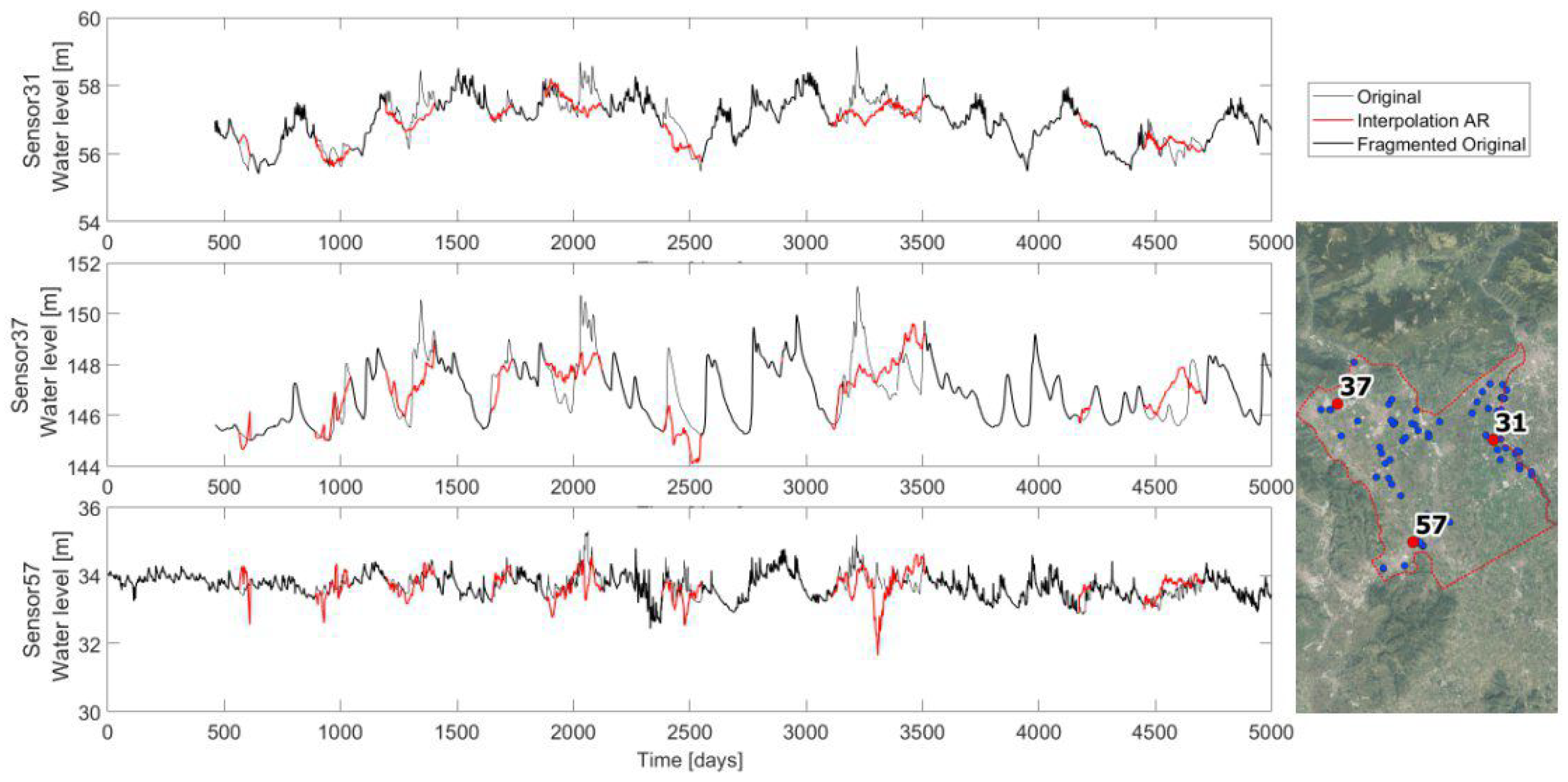
The interpolation is applied to the three long timeseries previously identified, and Figure 4 reports the resulting interpolations. Observing the graphs, it is noticeable how the interpolation can mimic the local hydrogeological behavior, even if sometimes it creates unreal minimums and peaks. This is due to the statistical approach that lacks hydrological knowledge and guidance.
Differently from the previous methods, the patched kriging (PK) is a geostatistical approach that takes advantage of the spatial information of the groundwater level. It has been originally proposed and implemented by [34] in order to deal with uneven and fragmented rainfall records that are useful for the statistical assessment of extremes. The method considers each measurement as a 3D point , and for each timestep, a spatial interpolation in the whole domain is carried out. This way, missing values in the timeseries can be evaluated owing to the concomitant information in other measurement points, extracting information from timeseries recorded nearby in space. To the authors’ knowledge, this method has been never applied to impute groundwater level timeseries. This technique evaluates the parameter value also in unmeasured points, but it is not a result of interest in this study.
Each measurement is considered as a 3D point for each time instant the hydraulic data are spatially interpolated. The method applied by [34] and by this study is the ordinary kriging. All details regarding kriging are extensively available in the geostatistical literature, e.g., [53]. Differently from the original study, the here applied PK method does not correct the data for elevation effects. The current analysis directly evaluates the spatial dependence of measured records by estimating a sample variogram as:
where L is the lag distance, and are observations lagged by a distance L, and is the number of pairs separated by lag L. As in [34], for each timestep, the sample variogram is evaluated by using Equation (4), and the global sample variogram is estimated as a weighted average of these. The weights are defined as the number of measuring points in each timestep. Then, the theoretical variogram is estimated with the exponential form best fitting the global sample variogram. The exponential model has been simply selected as first attempt, given the preliminary phase of this comparative study. This variogram model needs the definition of the nugget and the number of the considered nearest points: the nugget effect is neglected, and therefore, the measured values are preserved, while the latter parameter is arbitrary and there are different objects to look at in order to define it. It depends on the desired variability scale: few neighbors for identifying a small scale, and up to the whole sample if the small scale is not required and if a shorter computational time is desired. Ref. [54] suggest a number of between 10 and 20, even if this number should depend on the range of the evaluated variogram. In this study, as well as in [34], given that for each timestep the number and the spatial distribution of recording sensors varies, the variogram range has been used as a first hint for selecting the number of nearest points. Given the sensors’ spatial distribution within the domain and the estimated range, the algorithm always considers the 10 closest sensors for the kriging interpolation. In this manner, a minimum amount of information is also guaranteed also in areas with a lower density of sensors.
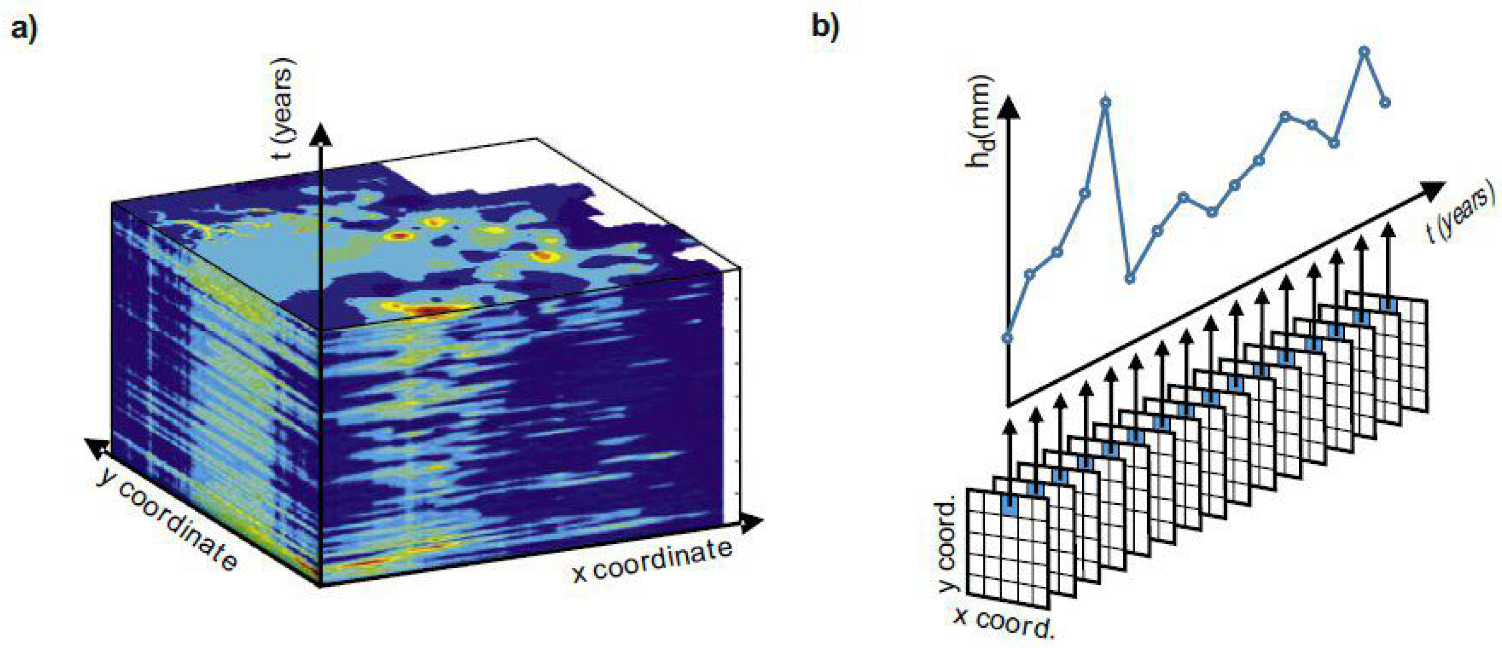
After the space interpolation and the creation of a map for each timestep with a space resolution of 25 m × 25 m, complete timeseries are extracted for each sensor location: i.e., given the space coordinates of a sensor , the complete series in the t axis is extracted from all maps, see Figure 5.
Moreover, the interpolated timeseries have to be further adjusted with respect to the procedure of [34]. The Extracted timeseries coincides with the recorded one when data are available, but it can be offset in interpolated gaps as the water level is driven by surrounding points that could have different average elevations. Nevertheless, the oscillations of the neighboring timeseries are significant information to be extracted by the spatial interpolation. Therefore, the timeseries are shifted in order to have the first interpolated value of the gap be coincident with the last known value (). Moreover, looking at the shifted timeseries, often it shows a step between the last shifted interpolated value and the first recorded value after the gap . This step can be upward, showing a hydrogeological peak, or downward, which is less realistic for a descending water level. Indeed, the ascending side of the hydrogeological peak can be very steep, while the descending one has always a slighter slope. A correction is applied only for the descendant phase () linearly modifying the interpolated series and making the two points coincide .
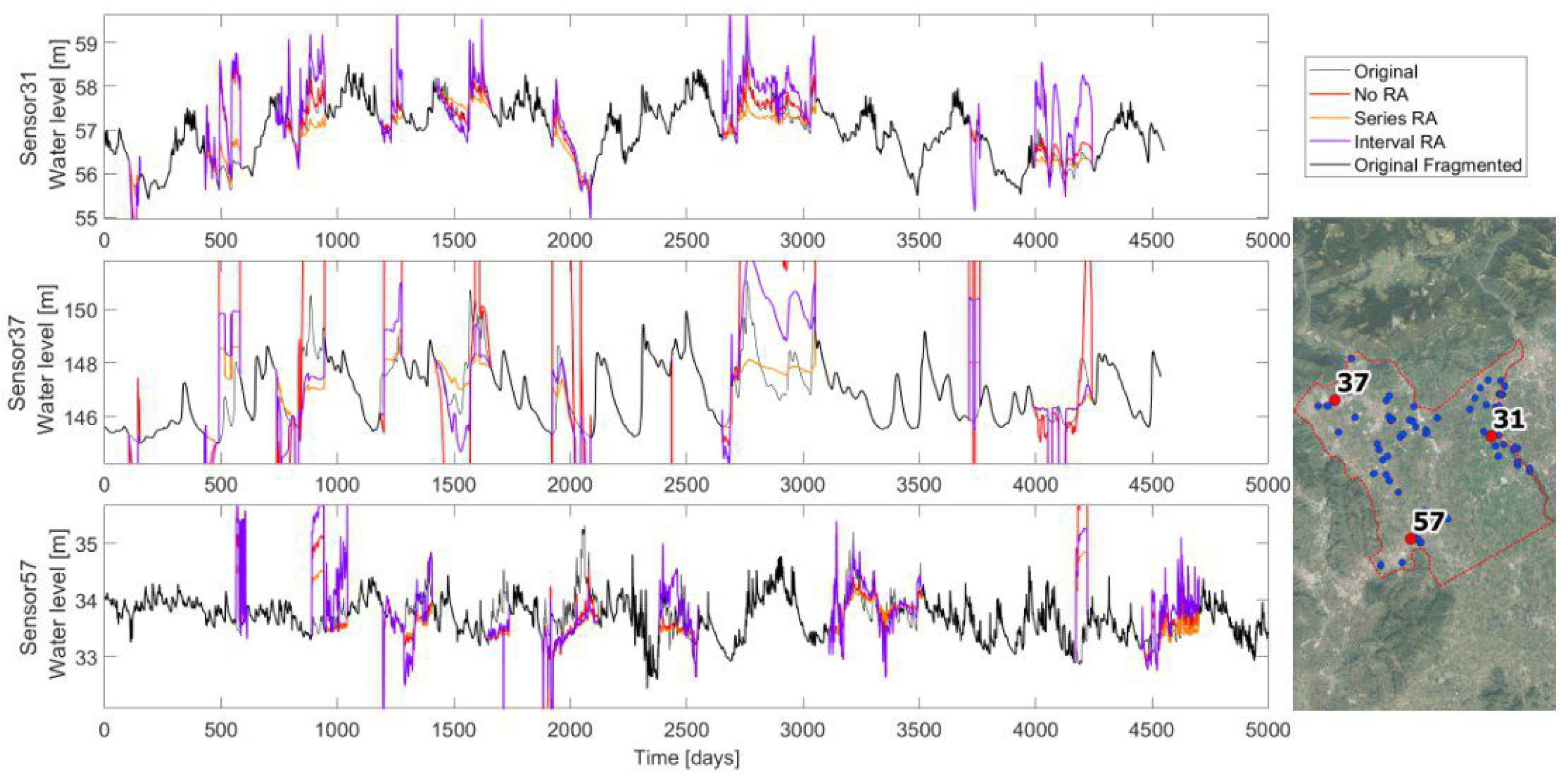
Another needed adjustment is made with regard to the oscillations range. Depending on the hydrogeological local connections, between the recording sensors, the oscillations range could be very different. In order to define which range adjustment (RA) to use, three possibilities are investigated and compared on imputing the three complete long timeseries. The three options are: (i) no range adjustment; (ii) series arrangement, meaning that the whole interpolated timeseries is proportionate in order to have the same range as the original fragmented timeseries; and (iii) interval arrangement, by proportioning the interpolated timeseries on each gap with the original record. Looking at the results comparison in Figure 6, different observations arise. In sensor 31, the PK works well on the reproduction of the real timeseries, and even with no range adjustment, the reconstructed timeseries well fits the reality in almost all gaps. This is probably due to the availability of many nearby surrounding points that well guide the imputation method. On the contrary, sensor 37 is not well reproduced and a range adjustment is necessary. The interval adjustment has water level oscillations that are close to the recorded ones, but they are shifted. The series adjustment is well located on average, the problem is that the fluctuations are softened. Finally, sensor 57 is similarly interpolated by the different range adjustments. In general, the interval RA has the tendency to enhance fluctuations, and not adjusted RA is sometimes the best option (sensor 31), even if occasionally it is completely out of the series range (sensor 37), while the series RA seems to be the safest option, even if it tends to soften the peaks. The best RA option is chosen by comparing the mean percentage daily errors, defined as the Euclidean distance divided by the total missing values of the series, and scaled based on the oscillations range:
where and are the interpolated and original timeseries, is the total number of missing values, and r is the recorded range of the original timeseries. The error is evaluated for each sensor and for each interpolation. Table 1 highlights as the interpolation with a series range of adjustment that better fits the original timeseries: it is always the minimum error. This RA is therefore chosen for the PK imputation method. Additionally, these results (particularly in the imputation of the timeseries of sensor 37) clearly show how sometimes the PK technique is step-shaped and where the applied shift procedure is not enough. This is probably because the imputed timeseries does not have so many recording sensors nearby, hence, it is sensitive to the activation and deactivation of the few surrounding points.
The last interpolation is the average of all previous imputation methods. Note that if the spline interpolation has been removed because it failed to respect the aforementioned range conditions, the average is only between the autoregressive linear model and the patched kriging methods.
2.4. Comparing Procedures and Applied Statistical Analyses
For an easy understanding of the imputation methods performances, the first procedure compares interpolations with true timeseries: the comparison in time domain that returns an immediate feeling of the interpolation’s goodness is easy to comprehend and evaluate, then statistical analyses are applied to see how sensitive these analyses are to the chosen imputation method. This comparison with the true timeseries is possible only for a few timeseries of the dataset: three series have been identified to be at least 12 years long, with less than of missing values, and located far away from each other in order to not bias the analysis. The identified timeseries are 31, 37, and 57, the locations of which are shown in Figure 2. The three timeseries have been fragmented in MATLAB by randomly creating 12 gaps, applying the functions randfixedsum e randi. The fragmentation procedure has been guided by removing of the shortest timeseries (1608 values), and it created variably long gaps ranging from 45 to 356 days.
The second procedure aims to compare the results of the imputation methods on the whole dataset, using all of the available timeseries to evaluate how much of the method is affecting the results of some statistical analyses. This returns an idea of the importance of correctly selecting the imputation method, even if the comparison with the reality is not possible. It is substantially a sensitivity analysis.
As a comparison of imputations, both procedures apply and compare the results of three statistical analyses, with the following being briefly described: Fourier analysis, autocorrelation, and microscale. The Fourier analysis provides a different view of timeseries because it analyses them in the frequency domain [55]. Its main result is the power spectrum that points out timeseries periodicities, which are usually not easily recognizable in the time domain. This result is often interesting for hydrogeological studies, as the main hydraulic periodicities depend on the most relevant hydraulic drivers affecting the site. The Discrete Fourier transform is carried out to move from the time to the frequency domain by applying the Fast Fourier Transform algorithm-fft function in MATLAB. The second statistical analysis is the evaluation of the autocorrelation function that defines the correlation (Pearson coefficient [53]) of a signal with a delayed copy of itself as a function of the time lag k. This analysis is usually useful for having insights on signal persistence and periodicity. The sample autocorrelation function (ACF) is defined by applying the autocorr function in MATLAB. The final analysis is the definition of an integral scale parameter, the microscale. It represents the time interval in which values are perfectly correlated, and it is an indication of the series memory and fluctuations rapidity. There are three ways to evaluate it:
- Using the formula of [56]:where is the autocorrelation value at , and is therefore equal to 1, and is its second derivative in 0;
- Evaluating the intersection with the abscissa axis of the parabola passing by point and leaned against the first autocorrelation values;
- Using Equation (6) but evaluating it starting from the parabola previously defined. Giving the parabola general equation , the formula becomes
3. Results and Discussion
3.1. Comparison on Three Complete Long Timeseries
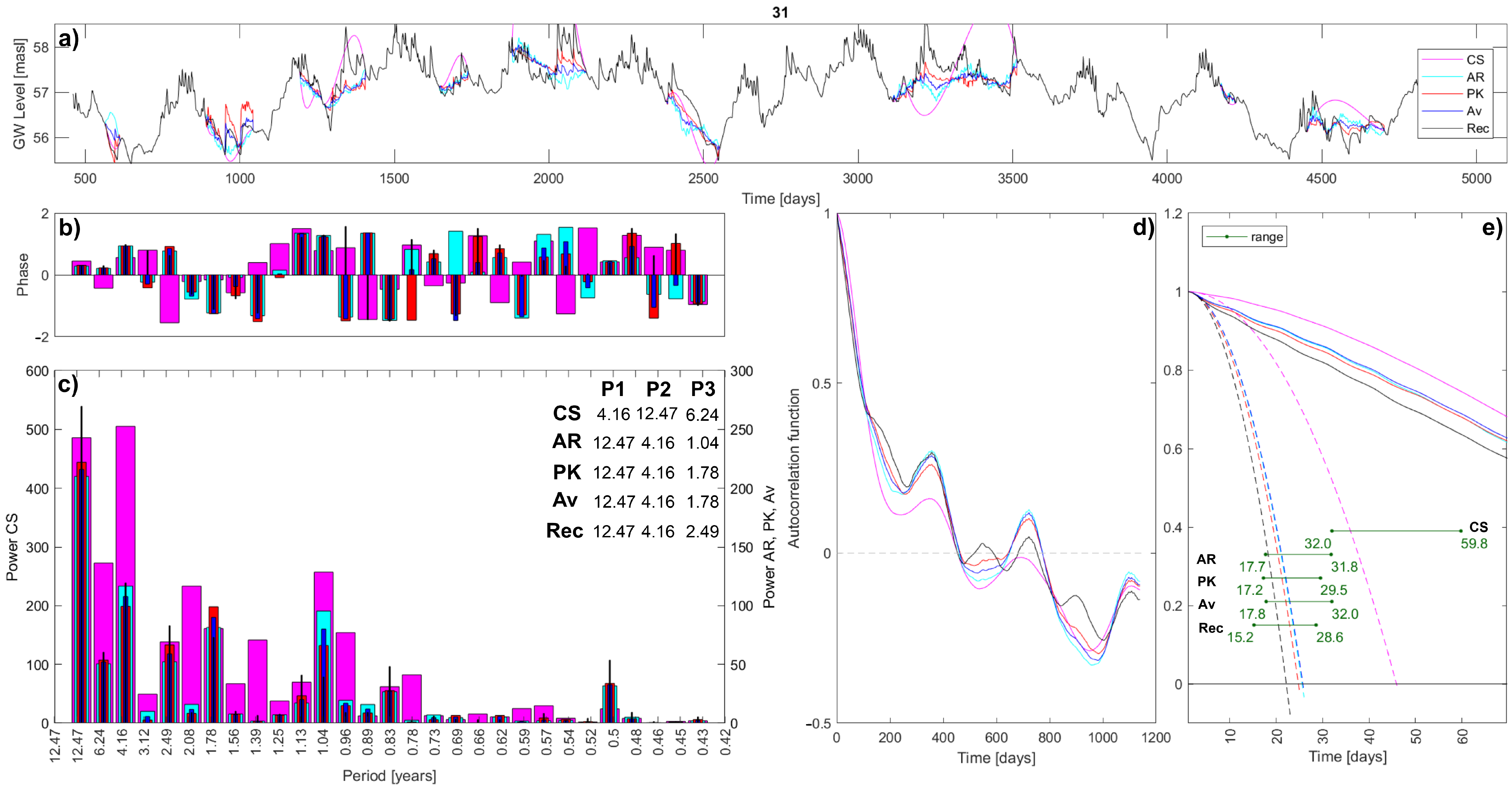
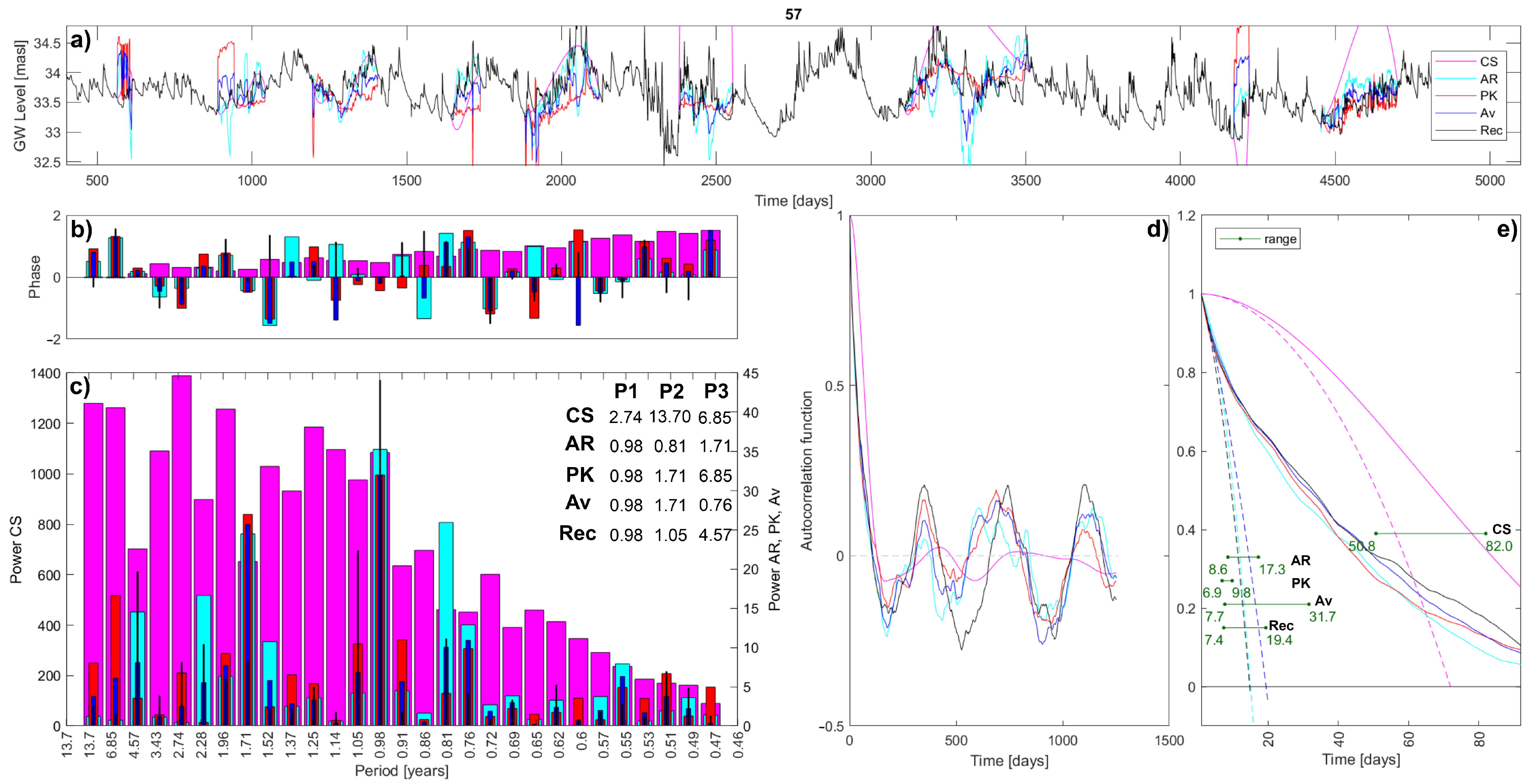
The results of the comparative analysis on the three chosen long timeseries are shown in Figure 7, Figure 8 and Figure 9. Plot ‘a’ shows the comparison in the time domain: the interpolations’ trend, compared to the known true trend. The cubic spline interpolation fails to properly reproduce the true record, owing to its smooth behavior and some outsize extreme values. All three reconstructed series do not meet the extremes condition; therefore, the CS interpolation should not be considered as a viable option. Its results are kept only in order to show the differences with other imputation methods. Regarding the autoregressive linear model, it creates a reasonable trend for all timeseries, meaning that its oscillations are similar to the recorded ones. However, the method is not hydrogeologically driven, and therefore, at times, it diverges in the opposite direction with respect to the removed observations. On the contrary, the patched kriging interpolation follows the real trend, given its hydrogeological basis. Close-by sensors and related information are obviously supporting the fitting of the input timeseries, and thus guiding the interpolated groundwater levels. Having one standalone borehole (with the closest neighbor being far away) could lead to erroneous imputations if different local stresses are present. Otherwise, the shifted interpolated data adjust the originally diverging groundwater level averages, and thus, it is likely to behave well. Instead, the main observed PK flaw is due to the activation or the deactivation of nearby recording points, affecting the induced water level in the interpolated point and producing a step-shaped behavior. The shifting correction solves many similar issues, but sometimes they tend to persist, degrading the overall imputation quality. The average interpolation is a compromise that reduces the PK stepped shape, even if it is sometimes still noticeable (e.g., sensor 37 in Figure 8), and maintains a clear hydrological meaning, thus improving the AR interpolation.
In order to confirm the observations by visual inspection and to assess how well the interpolated timeseries approximate the real recorded one, the R2 coefficient has been computed. They are shown in Table 2 for each method and each sensor. Obviously, an R2 of 1 indicates a perfect interpolation of the data. The CS method is poorly performing, while others compete with the PK for the best fitting. The PK performs better than any other method when it is not affected by the activation of neighboring sensors, i.e., when the interpolation is step-shaped. Moreover, within the tested timeseries, it is noticeable how sensor 57 is the most poorly imputed, maybe due to the fast groundwater level oscillations.
The Fourier analysis produces the phase and power spectra as results. The phase is reported in plots ‘b’, but it only shows and confirms the randomness of the process. The main result is the power spectrum, reported in plots ‘c’. Regarding the power spectra, firstly, it is evident how the CS interpolation is highly overestimating the magnitude, especially for sensors 37 and 57; secondly, its shape does not follow the true one. Looking at other interpolations instead, the magnitude is maintained, and the shape is quite similar too. These observations are confirmed by the R2 coefficient and are computed to assess how well the spectrum of each sensor approximates the real recorded one: the CS method is poorly performing, while PK best performs for fitting the spectra of sensors 31 and 37. As for the comparison in the time domain, sensor 57 is the most poorly imputed. Nevertheless, slightly different understandings come from the tables reported within the graph where the three main periodicities are identified. Not considering the CS interpolation, the tables show how all imputation methods lead to the correct identification of the two main periodicities for sensor 31 and the main periodicity for sensor 57. While for sensor 37, only the PK succeeds on identifying the main periodicity. In conclusion, AR, KP, and the average interpolations are relatively good at reproducing the magnitude and shape of the power spectrum, but on the specific action of identification for the main periodicities, they are less reliable.
Regarding the autocorrelation analysis, the resulting functions are reported in plots ‘d’. Except for the CS function that is always the farthest, other interpolations have similar autocorrelation functions that decently reproduce the function of the original timeseries. For each imputation method, the distance from the true autocorrelation function has been evaluated as the mean Euclidean distance:
where: and are respectively the interpolated and the true autocorrelation functions; and is the length of autocorrelation functions. Table 3 reports the evaluated distances and highlights that the PK interpolation has the closest autocorrelation function to the true one. Its distances are the lowest for sensors 31 and 37. For sensor 57, the average interpolation has the minimum distance, but the PK distance is very close. The same conclusions can be derived by calculating the R2 coefficient: the CS is the poorest performer, while the PK always has the highest coefficients.
In plots ‘e’, the microscale is shown as a range because there exist multiple applicable methods to compute it, see Section 2.4. As a consequence, interpolations differ on the minimum, mean, and maximum evaluated microscales, but also in the range extent. As for other analyses, the results of the CS interpolation are far from the true outcome, and also far from the ones of all other interpolations. Indeed, its microscale evaluation is too high for all sensors, while other methods provide closer estimations: the order of magnitude is well identified, even if the range slightly differs. No general patterns are identified, and the interpolations results differ, depending on the sensor analyzed.
Finally, the CS interpolation proves to be unsuitable, both in the time domain and in terms of the statistical analyses. This is likely due to the presence of large gaps in the fragmented timeseries that cause high interpolated peaks that should be removed. Comparing the results of other imputation methods, the PK returns results that are close to reality for the Fourier analysis and the autocorrelation function, but its weak point is the occasional stepped behavior in time that is surely not realistic. The AR has good performances on statistical results and a reasonable trend in the time domain, even though it lacks hydrogeological bases. The average interpolation softens both the pros and the cons of these last two imputation methods by considering both the hydrogeological guide of PK and the reasonable timeseries rendering of AR. Nevertheless, given the general performance dependence on the gap’s length and position, in addition to the sensor analyzed, these results are useful for an understanding of the method, but hardly suited to the general conclusions.
3.2. Comparison on the Whole Dataset of the Recorded Timeseries
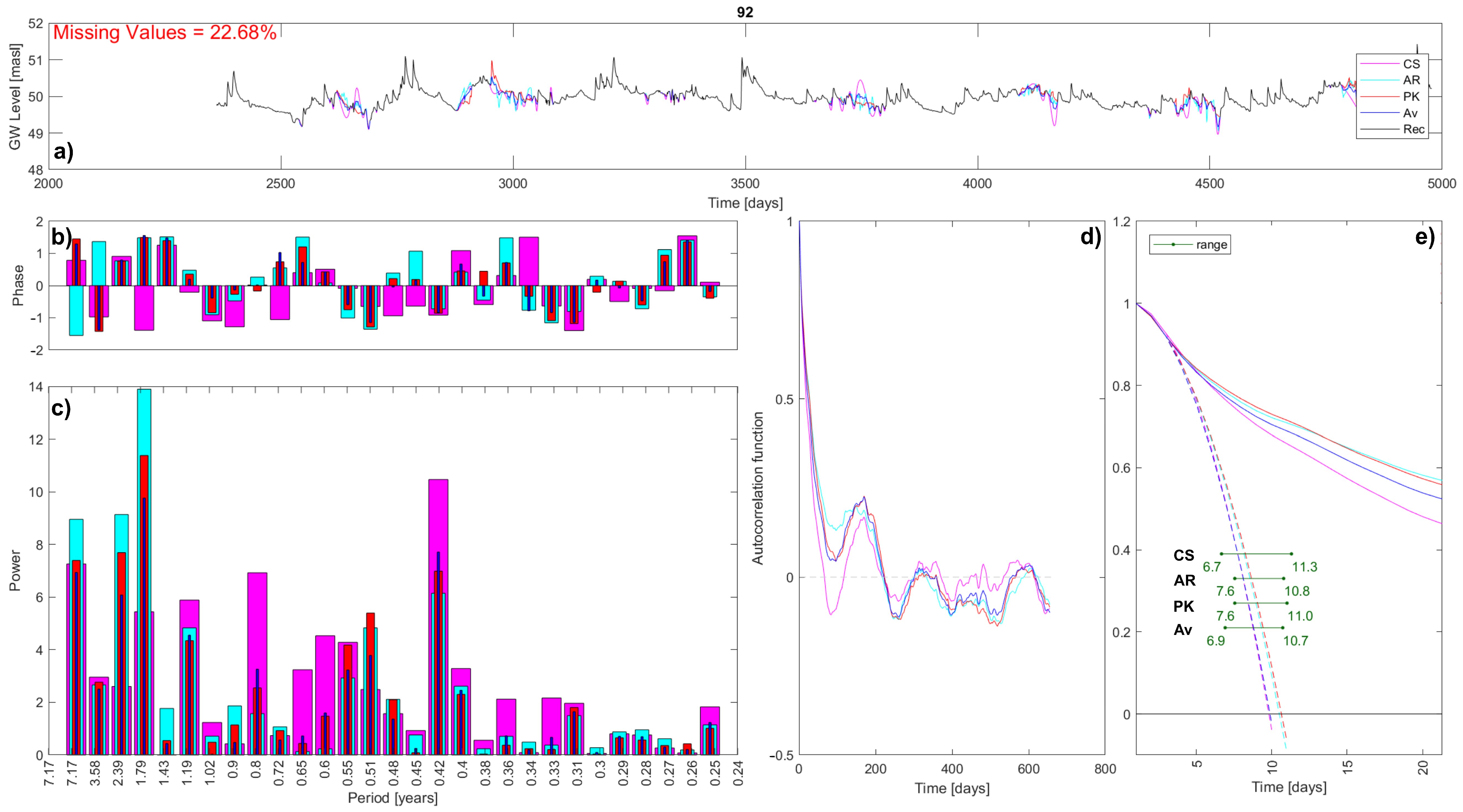
In order to obtain some conclusions that are specifically aimed at selecting the proper imputation method, the same three statistical analyses (Fourier analysis, autocorrelation, and microscale evaluation) are applied to the whole dataset of 79 records for which missing values are present and true timeseries are unknown. Note that 26 series have no missing values, and the remaining 53 series are the focus of this analysis. In order to observe the variability of the statistical results depending on the selected method, indicators are defined and applied to evaluate the statistical variability for each sensor in the dataset. These general indicators allow for a comparison of the results variability within the dataset. Indicators are thus presented and applied, as an example, to sensor 92, whose data and statistical figures are reported in Figure 10.
For the Fourier analysis, the main result concerns the power spectrum that pinpoints the main periodicities shown by the data. Interpolations affect the peak recognition; hence, the variability indicator is defined based on the identifiers of spectral peaks. Specifically, for each interpolation, the five main peaks are ordered by decreasing power, and the table is standardized by allowing for a fair comparison; see Table 4 and Table 5. The first table’s values are divided by the maximum period of the power spectrum, years in this example, and the standardized table is likewise constructed. The variance of each standardized period is then calculated and reported (in blue) in Table 5. In conclusion, the final indicator is defined as the mean of the five estimated peak variances: for sensor 92.
Regarding the autocorrelation function, the results’ variability is evaluated as the average maximum range along the function: the mean maximum distance. Specifically, for each time lag k, the autocorrelation functions with maximum and minimum values are identified, and the Euclidean distance is evaluated. The k distances are summed up and divided by the length of the autocorrelation function in order to standardize the indicator, thus allowing for the comparison within the dataset.
Finally, in order to evaluate, for each timeseries, the variability obtained in the evaluation of the microscale, different factors may be relevant. Depending on the specific goal, the maximum, minimum, mean, or range of the estimated microscale could be of interest. As a variability index, the coefficient of variation, , is calculated for each sensor s as:
Therefore, each microscale indicator is evaluated as the standard deviation of the maximum/minimum/mean/range values, estimated starting from the four interpolated timeseries, divided by their mean , as a standardization process. Table 6 reports the calculations steps for sensor 92.
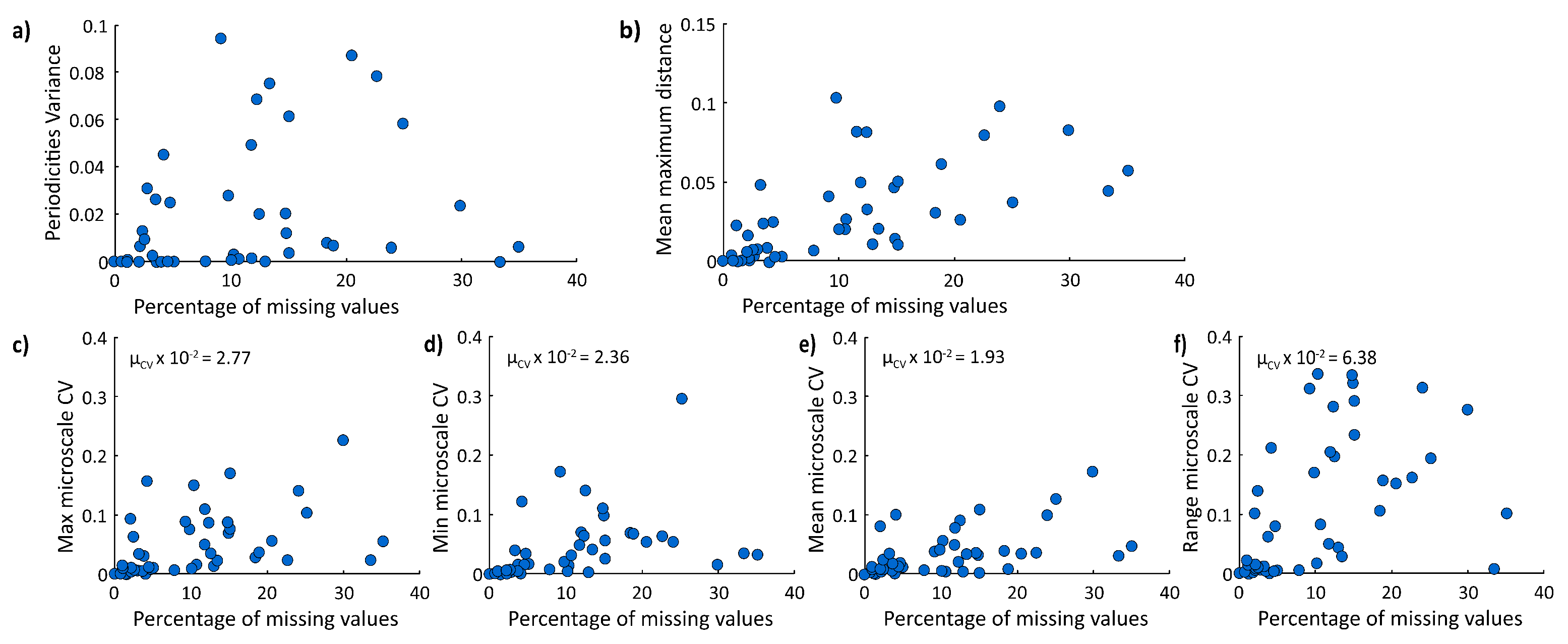
The six proposed variability indicators (one for the Fourier analysis, one for the autocorrelation, and four for the microscale) have been standardized in order to compare the results fairly for the whole dataset. The expectation is a positive dependence of each indicator variability on the percentage of missing values of the analyzed timeseries. Indeed, more missing values would imply a possibly major impact of the choice of imputation method. The variability indicator of the dataset is shown in Figure 11, plotted against the percentage of missing values.
By looking at the scatter plots, the variability of the six indicators may be evaluated. The periodicities variance and the mean maximum distance of the autocorrelation function have lower magnitudes than microscale indicators. However, they are not easily comparable because of the different standardization procedures. The comparison is possible between microscale indicators: the mean microscale is the indicator that is less dispersed, meaning that it is less affected by the chosen method, while the range is the most variable. Microscale observations are also confirmed by observing the indicator mean of the whole dataset, reported on the plots ‘c’ to ‘f’ in Figure 11.
Additionally, as expected, indicators are directly dependent on the percentage of missing values: it is noticeable a heteroskedastic behavior, i.e., the variance of the variability indicator is not homogeneous, but it varies depending on the values plotted in the x-axis. Heteroskedasticity is not always evident for the presence of a few outliers that bias the visual inspection.
The Fourier analysis indicator is the variance of the recognized most important periodicities. The real main periodicities are unknown, but the maximum variance between the timeseries is . Only two points are outliers, meaning that for them, the imputation method’s choice is affecting the statistical result more than the general dataset’s behavior. This statistical analysis seems to be ‘robust’ for the analyzed dataset, and the applied method does not excessively affect the result. Moreover, the periodicities variance indicator has been plotted on the map in Figure 12a to observe if any geographical trend is present. No specific trends are observed. For example, the proximity to timeseries with lower percentages of missing data does not lower the value of the variability indicator. The autocorrelation variability is evaluated by calculating the mean distance between the locally maximum and minimum functions. The maximum value evaluated in the dataset is below . The low distance values indicate quite robust results for this statistical analysis, as out of a range represents an error of . Thus, even this statistical analysis seems to be ‘robust’ for the analyzed dataset. Regarding the microscale analysis, between the four indicators, the mean microscale is the one that is less variable, and with lower CVs, for high missing data percentages. Thus, the mean microscale seems to be the most robust to the different applied imputation methods.
It is likely that different types of missing data can differentially affect the results of the various imputation methods. Missing point data is not an issue, but longer gaps can strongly affect any imputation result. Moreover, in addition to the length of every single gap, the results of the imputation methods are significantly impacted by the missing data forms: i.e., how often and in which hydrogeological moment (low, high, or average groundwater level) the missing data are present. Future works should investigate the sensitivity of imputation methods to the different missing data forms.
This study presented and compared different simple-to-implement methods tackling a common issue encountered by groundwater practitioners and highlighting their cons and pros on the applicability and the final fitting. With these results in mind, a groundwater practitioner can select with critical awareness the imputation method to apply. Based on such results, for this specific groundwater system, the authors decided to prefer the PK method if it is not step-shaped for the specific timeseries. In case it is not suitable, the Average method is the second choice if it manages to cancel the steps, otherwise the AR method is used. In this specific study, for the 53 timeseries with missing values: the PK method has been selected 41 times (), the average 5 times (), and the AR method, the remaining 7 times (). Figure 12b shows in which location each method has been preferred to the others, highlighting how the patched kriging dominates in the southern confined aquifer, while the three imputation methods alternate on the northern unconfined aquifer with no evident geographic trends. The PK method is preferred to other imputation methods (time imputation), even for some standalone boreholes, meaning that the concomitant information recorded by other sensors (even if far away) is useful for the imputation. Moreover, as the study objective is to support a proper imputation of the groundwater level timeseries, a forward step will be to provide a ready-to-use software for practitioners implementing an open source Python package including such imputation methods, as was performed with Pastas for the analysis of hydrogeological timeseries [11,12].
4. Conclusions
The present study compared three different imputation methods (Cubic Spline CS, Autoregressive linear model AR, and Patched Kriging PK) and their averages for groundwater level. The methods have been selected as they are relatively simple to implement in an automatic structure; hence, they are easily applicable for large datasets, and are potentially widely accessible to groundwater practitioners.
Although the method’s complexity increases going from CS, through AR to the PK, the latter imputation method is suggested to be the most appropriate method to interpolate the timeseries of the groundwater level, largely because of its ability to use information on the spatial correlation of the data. By comparing the results of the applied methods with the three true timeseries, the study concludes that: (i) the spline interpolation is the simplest to implement, but it is the poorest performing option; (ii) the autoregressive linear model is always hydrogeologically reasonable but it is not guided, and it is therefore missing relevant hydrological peaks or minimums; (iii) the patched kriging proves to be the best option, because it is hydrogeologically driven but also sensitive to the activation of neighboring sensors. The ensemble average of these methods is shown to be a good compromise between PK and AR as it retains the PK hydrogeological guide but softens the step-shaped trend by averaging with the AR trend.
Regarding the importance of properly choosing the imputation method, such an understanding is complex, and here it is based on the observation of the variabilitues of methods in a few statistical results of interpolated timeseries. Even if the outcome is uncertain, the comparative procedure on the whole available dataset highlights as the Fourier analysis, and the autocorrelation functions fail to be significantly sensitive to the selected interpolation method, while between microscale indicators, the mean microscale is the one that is less sensitive. Nevertheless, depending on the use of interpolated timeseries, more or less caution is necessary for the choice of the interpolation method: a site-specific and statistic-specific sensitivity analysis could be a useful preliminary step for relevant studies.
Author Contributions
Conceptualization, M.M. and A.R.; methodology, A.R.; software, M.M.; validation, G.P.; formal analysis, M.M.; investigation, M.M., S.B. and A.S.; resources, S.B. and A.S.; data curation, M.M.; writing—original draft preparation, M.M.; writing—review and editing, G.P., S.B., A.S. and A.R.; visualization, M.M.; supervision, A.R.; project administration, A.R.; funding acquisition, A.S. and A.R. All authors have read and agreed to the published version of the manuscript.
Funding
This research received no external funding.
Data Availability Statement
Proprietary database of Sinergeo srl.
Conflicts of Interest
The authors declare no conflict of interest.
References
- Vörösmarty, C.; McIntyre, P.; Gessner, M.; Dudgeon, D.; Prusevich, A.; Green, P.; Glidden, S.; Bunn, S.; Sullivan, C.; Liermann, R.; et al. Rivers in crisis: Global water insecurity for humans and biodiversity. Nature 2010, 467, 555–561. [Google Scholar] [CrossRef] [PubMed] [Green Version]
- Wheater, H.S.; Gober, P. Water security and the science agenda. Water Resour. Res. 2015, 51, 5406–5424. [Google Scholar] [CrossRef]
- Gleeson, T.; Alley, W.M.; Allen, D.M.; Sophocleous, M.A.; Zhou, Y.; Taniguchi, M.; VanderSteen, J. Towards sustainable groundwater use: Setting long-term goals, backcasting, and managing adaptively. Groundwater 2012, 50, 19–26. [Google Scholar] [CrossRef] [PubMed]
- Carrard, N.; Foster, T.; Willetts, J. Groundwater as a source of drinking water in southeast Asia and the Pacific: A multi-country review of current reliance and resource concerns. Water 2019, 11, 1605. [Google Scholar] [CrossRef] [Green Version]
- Elshall, A.S.; Arik, A.D.; El-Kadi, A.I.; Pierce, S.; Ye, M.; Burnett, K.M.; Wada, C.A.; Bremer, L.L.; Chun, G. Groundwater sustainability: A review of the interactions between science and policy. Environ. Res. Lett. 2020, 15, 093004. [Google Scholar] [CrossRef]
- Megdal, S.B.; Eden, S.; Shamir, E. Water Governance, Stakeholder Engagement, and Sustainable Water Resources Management. Water 2017, 9, 190. [Google Scholar] [CrossRef] [Green Version]
- Taylor, C.J.; Alley, W.M. Ground-Water-Level Monitoring and the Importance of Long-Term Water-Level Data; US Geological Survey: Denver, CO, USA, 2001; Volume 1217.
- Butler, J., Jr.; Stotler, R.; Whittemore, D.; Reboulet, E. Interpretation of water level changes in the High Plains aquifer in western Kansas. Groundwater 2013, 51, 180–190. [Google Scholar] [CrossRef]
- Zhang, Q.; López, D.L. Use of Time Series Analysis to Evaluate the Impacts of Underground Mining on the Hydraulic Properties of Groundwater of Dysart Woods, Ohio. Mine Water Environ. 2019, 38, 566–580. [Google Scholar] [CrossRef]
- Meggiorin, M.; Bullo, P.; Accoto, V.; Passadore, G.; Sottani, A.; Rinaldo, A. Applying the Principal Component Analysis for a deeper understanding of the groundwater system: Case study of the Bacchiglione Basin (Veneto, Italy). Acque-Sotter.-Ital. J. Groundw. 2022, 11, 7–17. [Google Scholar] [CrossRef]
- Collenteur, R.A.; Bakker, M.; Caljé, R.; Klop, S.A.; Schaars, F. Pastas: Open source software for the analysis of groundwater time series. Groundwater 2019, 57, 877–885. [Google Scholar] [CrossRef]
- Bakker, M.; Schaars, F. Solving groundwater flow problems with time series analysis: You may not even need another model. Groundwater 2019, 57, 826–833. [Google Scholar] [CrossRef] [PubMed] [Green Version]
- Hasanuzzaman, M.; Song, X.; Han, D.; Zhang, Y.; Hussain, S. Prediction of groundwater dynamics for sustainable water resource management in Bogra District, Northwest Bangladesh. Water 2017, 9, 238. [Google Scholar] [CrossRef] [Green Version]
- Cianflone, G.; Vespasiano, G.; De Rosa, R.; Dominici, R.; Apollaro, C.; Vaselli, O.; Pizzino, L.; Tolomei, C.; Capecchiacci, F.; Polemio, M. Hydrostratigraphic Framework and Physicochemical Status of Groundwater in the Gioia Tauro Coastal Plain (Calabria—Southern Italy). Water 2021, 13, 3279. [Google Scholar] [CrossRef]
- Islam, M.; Van Camp, M.; Hossain, D.; Sarker, M.M.R.; Khatun, S.; Walraevens, K. Impacts of large-scale groundwater exploitation based on long-term evolution of hydraulic heads in Dhaka city, Bangladesh. Water 2021, 13, 1357. [Google Scholar] [CrossRef]
- Meggiorin, M.; Passadore, G.; Bertoldo, S.; Sottani, A.; Rinaldo, A. Assessing the long-term sustainability of the groundwater resources in the Bacchiglione basin (Veneto, Italy) with the Mann-Kendall test: Suggestions for higher reliability. Acque-Sotter.-Ital. J. Groundw. 2021, 10, 35–48. [Google Scholar] [CrossRef]
- Viaroli, S.; Lotti, F.; Mastrorillo, L.; Paolucci, V.; Mazza, R. Simplified two-dimensional modelling to constrain the deep groundwater contribution in a complex mineral water mixing area, Riardo Plain, southern Italy. Hydrogeol. J. 2019, 27, 1459–1478. [Google Scholar] [CrossRef] [Green Version]
- Meggiorin, M.; Passadore, G.; Sottani, A.; Rinaldo, A. Understanding the importance of hydraulic head timeseries for calibrating a flow model: Application to the real case of the Bacchiglione Basin. In Proceedings of the EGU General Assembly Conference Abstracts, Online, 4–8 May 2020; p. 5938. [Google Scholar]
- Chen, L.; Wang, X.; Liang, G.; Zhang, H. Evaluation of Groundwater Flow Changes Associated with Drainage within Multilayer Aquifers in a Semiarid Area. Water 2022, 14, 2679. [Google Scholar] [CrossRef]
- Polomčić, D.; Bajić, D.; Hajdin, B.; Pamučar, D. Numerical Modeling and Simulation of the Effectiveness of Groundwater Source Protection Management Plans: Riverbank Filtration Case Study in Serbia. Water 2022, 14, 1993. [Google Scholar] [CrossRef]
- Ntona, M.M.; Busico, G.; Mastrocicco, M.; Kazakis, N. Modeling groundwater and surface water interaction: An overview of current status and future challenges. Sci. Total. Environ. 2022, 846, 157355. [Google Scholar] [CrossRef]
- Nunes, L.; Cunha, M.; Ribeiro, L. Groundwater monitoring network optimization with redundancy reduction. J. Water Resour. Plan. Manag. 2004, 130, 33–43. [Google Scholar] [CrossRef] [Green Version]
- Hosseini, M.; Kerachian, R. A data fusion-based methodology for optimal redesign of groundwater monitoring networks. J. Hydrol. 2017, 552, 267–282. [Google Scholar] [CrossRef]
- Sottani, A.; Meggiorin, M.; Ribeiro, L.; Rinaldo, A. Comparison of two methods for optimizing existing groundwater monitoring networks: Application to the Bacchiglione Basin, Italy. In Proceedings of the EGU General Assembly Conference Abstracts, Online, 4–8 May 2020; p. 8759. [Google Scholar]
- Garamhegyi, T.; Hatvani, I.G.; Szalai, J.; Kovács, J. Delineation of Hydraulic Flow Regime Areas Based on the Statistical Analysis of Semicentennial Shallow Groundwater Table Time Series. Water 2020, 12, 828. [Google Scholar] [CrossRef] [Green Version]
- Naranjo-Fernández, N.; Guardiola-Albert, C.; Aguilera, H.; Serrano-Hidalgo, C.; Montero-González, E. Clustering groundwater level time series of the exploited Almonte-Marismas aquifer in Southwest Spain. Water 2020, 12, 1063. [Google Scholar] [CrossRef] [Green Version]
- Flinck, A.; Folton, N.; Arnaud, P. Assimilation of Piezometric Data to Calibrate Parsimonious Daily Hydrological Models. Water 2021, 13, 2342. [Google Scholar] [CrossRef]
- Kayhomayoon, Z.; Babaeian, F.; Ghordoyee Milan, S.; Arya Azar, N.; Berndtsson, R. A Combination of Metaheuristic Optimization Algorithms and Machine Learning Methods Improves the Prediction of Groundwater Level. Water 2022, 14, 751. [Google Scholar] [CrossRef]
- Yu, H.; Yu, C.; Ma, Y.; Zhao, B.; Yue, C.; Gao, R.; Chang, Y. Determining Stress State of Source Media with Identified Difference between Groundwater Level during Loading and Unloading Induced by Earth Tides. Water 2021, 13, 2843. [Google Scholar] [CrossRef]
- Minderhoud, P.; Erkens, G.; Pham, V.; Bui, V.T.; Erban, L.; Kooi, H.; Stouthamer, E. Impacts of 25 years of groundwater extraction on subsidence in the Mekong delta, Vietnam. Environ. Res. Lett. 2017, 12, 064006. [Google Scholar] [CrossRef]
- Carneiro, J.; Carvalho, J. Groundwater modelling as an urban planning tool: Issues raised by a small-scale model. Q. J. Eng. Geol. Hydrogeol. 2010, 43, 157–170. [Google Scholar] [CrossRef]
- Patra, S.; Sahoo, S.; Mishra, P.; Mahapatra, S.C. Impacts of urbanization on land use/cover changes and its probable implications on local climate and groundwater level. J. Urban Manag. 2018, 7, 70–84. [Google Scholar] [CrossRef]
- Feng, L.; Nowak, G.; O’Neill, T.; Welsh, A. CUTOFF: A spatio-temporal imputation method. J. Hydrol. 2014, 519, 3591–3605. [Google Scholar] [CrossRef]
- Libertino, A.; Allamano, P.; Laio, F.; Claps, P. Regional-scale analysis of extreme precipitation from short and fragmented records. Adv. Water Resour. 2018, 112, 147–159. [Google Scholar] [CrossRef]
- Ginocchi, M.; Crosta, G.; Rotiroti, M.; Bonomi, T. Analysis and prediction of groundwater level time series with Autoregressive Linear Models. Rend. Online Della Soc. Geol. Ital. 2016, 39, 109–112. [Google Scholar] [CrossRef]
- Taie Semiromi, M.; Koch, M. Reconstruction of groundwater levels to impute missing values using singular and multichannel spectrum analysis: Application to the Ardabil Plain, Iran. Hydrol. Sci. J. 2019, 64, 1711–1726. [Google Scholar] [CrossRef]
- Guo, T.; Song, S.; Yan, Y. A time-varying autoregressive model for groundwater depth prediction. J. Hydrol. 2022, 613, 128394. [Google Scholar] [CrossRef]
- Krishna, B.; Satyaji Rao, Y.; Vijaya, T. Modelling groundwater levels in an urban coastal aquifer using artificial neural networks. Hydrol. Process. Int. J. 2008, 22, 1180–1188. [Google Scholar] [CrossRef]
- Mohanty, S.; Jha, M.K.; Kumar, A.; Sudheer, K. Artificial neural network modeling for groundwater level forecasting in a river island of eastern India. Water Resour. Manag. 2010, 24, 1845–1865. [Google Scholar] [CrossRef]
- Park, J.; Muller, J.; Arora, B.; Faybishenko, B.; Pastorello, G.; Varadharajan, C.; Sahu, R.; Agarwal, D. Long-Term Missing Value Imputation for Time Series Data Using Deep Neural Networks. arXiv 2022, arXiv:2202.12441. [Google Scholar] [CrossRef]
- Yan, Q.; Ma, C. Application of integrated RIMA and RBF network for groundwater level forecasting. Environ. Earth Sci. 2016, 75, 396. [Google Scholar] [CrossRef]
- Asgharinia, S.; Petroselli, A. A comparison of statistical methods for evaluating missing data of monitoring wells in the Kazeroun Plain, Fars Province, Iran. Groundw. Sustain. Dev. 2020, 10, 100294. [Google Scholar] [CrossRef]
- He, L.; Chen, S.; Liang, Y.; Hou, M.; Chen, J. Infilling the missing values of groundwater level using time and space series: Case of Nantong City, east coast of China. Earth Sci. Inform. 2020, 13, 1445–1459. [Google Scholar] [CrossRef]
- Smith, T.M.; Reynolds, R.W.; Livezey, R.E.; Stokes, D.C. Reconstruction of historical sea surface temperatures using empirical orthogonal functions. J. Clim. 1996, 9, 1403–1420. [Google Scholar] [CrossRef]
- Dwivedi, D.; Mital, U.; Faybishenko, B.; Dafflon, B.; Varadharajan, C.; Agarwal, D.; Williams, K.H.; Steefel, C.I.; Hubbard, S.S. Imputation of contiguous gaps and extremes of subhourly groundwater time series using random forests. J. Mach. Learn. Model. Comput. 2022, 3, 1–22. [Google Scholar] [CrossRef]
- Zhang, Z.; Yang, X.; Li, H.; Li, W.; Yan, H.; Shi, F. Application of a novel hybrid method for spatiotemporal data imputation: A case study of the Minqin County groundwater level. J. Hydrol. 2017, 553, 384–397. [Google Scholar] [CrossRef]
- Razzagh, S.; Sadeghfam, S.; Nadiri, A.; Busico, G.; Ntona, M.; Kazakis, N. Formulation of Shannon entropy model averaging for groundwater level prediction using artificial intelligence models. Int. J. Environ. Sci. Technol. 2021, 19, 6203–6220. [Google Scholar] [CrossRef]
- Pappas, C.; Papalexiou, S.M.; Koutsoyiannis, D. A quick gap filling of missing hydrometeorological data. J. Geophys. Res. Atmos. 2014, 119, 9290–9300. [Google Scholar] [CrossRef]
- Dal Prà, A.; Bellatti, R.; Costacurta, R.; Sbettega, G. Distribuzione Delle Ghiaie nel Sottosuolo Della Pianura Veneta; Quaderni IRSA e del Consiglio Nazionale delle Ricerche; IRSA: Rome, Italy, 1976. [Google Scholar]
- Passadore, G.; Monego, M.; Altissimo, L.; Sottani, A.; Putti, M.; Rinaldo, A. Alternative conceptual models and the robustness of groundwater management scenarios in the multi-aquifer system of the Central Veneto Basin, Italy. Hydrogeol. J. 2012, 20, 419. [Google Scholar] [CrossRef]
- De Boor, C. A Practical Guide to Splines; Springer: New York, NY, USA, 1978; Volume 27. [Google Scholar]
- Ginocchi, M. Studio Esplorativo di Serie Storiche Idrologiche. Master’s Thesis, Università degli Studi di Milano-Bicocca, Milan, Italy, 2014. [Google Scholar]
- Isaaks, E.H.; Srivastava, R.M. Applied Geostatistics; Oxford University Press: Oxford, UK, 1989. [Google Scholar]
- Kolárová, M.; Hamouz, P. Approaches to the analysis of weed distribution. In Atlas of Weed Mapping; Kraehmer, H., Ed.; John Wiley & Sons, Inc.: New York, NY, USA, 2016; pp. 440–455. [Google Scholar]
- Bras, L.R.; Rodriguez-Iturbe, I. Random Functions and Hydrology; Dover Publications: Mineola, NY, USA, 1994. [Google Scholar]
- Batchelor, G.K. The Theory of Homogeneous Turbulence; Cambridge University Press: Cambridge, UK, 1953. [Google Scholar]
Figure 1.
Flowchart of the analysis applied to compare the results of the imputation methods: pre-processing phase, imputation phase applying three different methods and their average for the interpolation of missing values, the comparison phase comprising two parallel procedures working on different datasets (three complete long timeseries vs. the whole dataset), and both comparing the results of three statistical analyses on the imputed timeseries. Blue squares and arrows define the main phases of the analysis.

Figure 2.
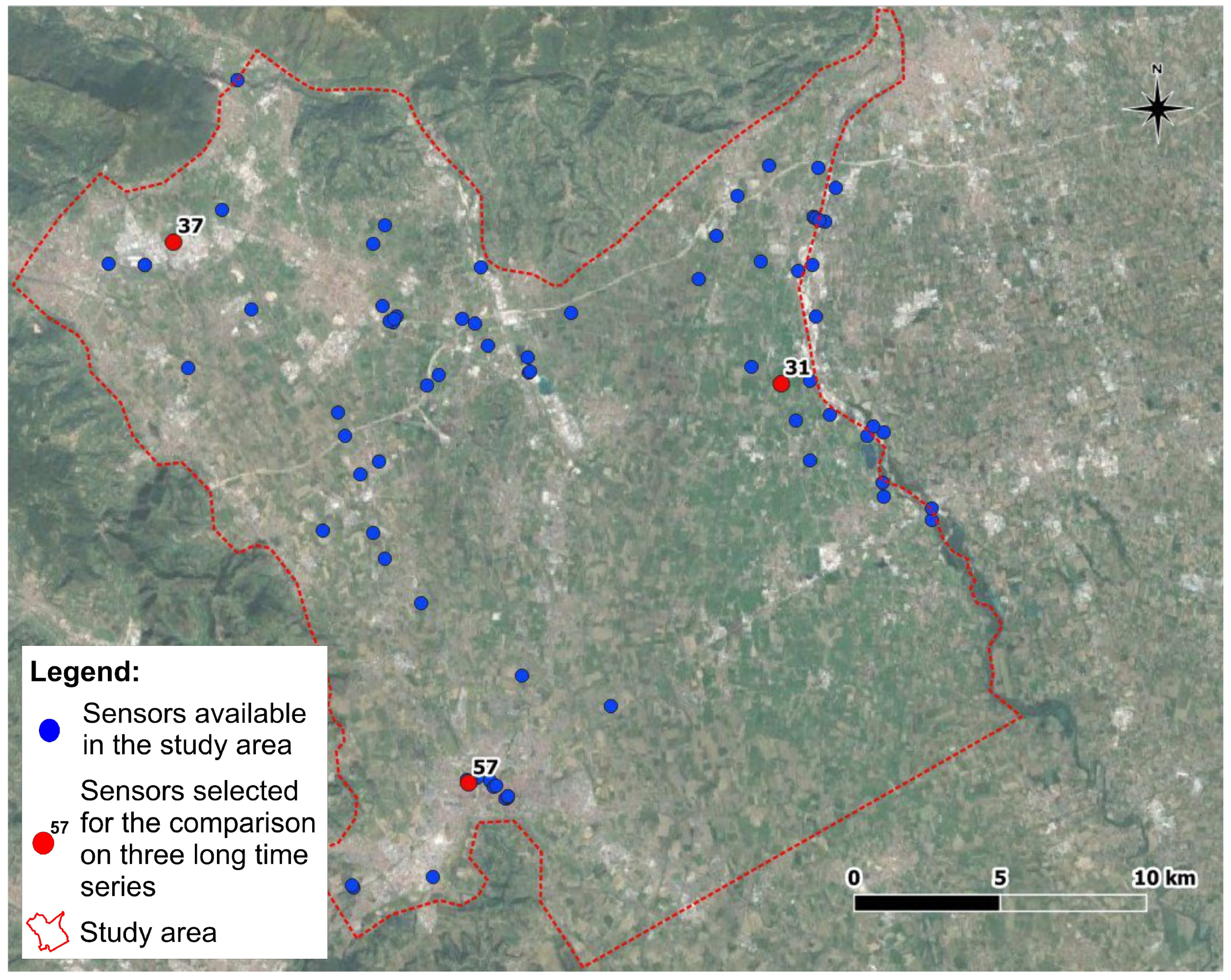
Map of the sensors within the study area: the 79 sensors included in the pre-processed dataset (blue) and the three identified sensors for the first comparative procedure on complete long timeseries (red).
Figure 2.
Map of the sensors within the study area: the 79 sensors included in the pre-processed dataset (blue) and the three identified sensors for the first comparative procedure on complete long timeseries (red).

Figure 3.
Cubic Spline interpolation applied to the three timeseries (sensors 31, 37, and 57). For each sensor, a plot shows the comparison of the original complete recorded timeseries (in gray) with the interpolated timeseries (in red) of the fragmented timeseries (in black). On the right, the map shows the location of the three sample timeseries within the domain.

Figure 4.
The autoregressive linear model applied to the three long timeseries (sensors 31, 37, and 57). For each sensor, a plot shows the comparison of the original complete recorded timeseries (in gray) with the interpolated timeseries (in red) of the fragmented timeseries (in black). On the right, the map shows the locations of the three sample timeseries within the domain.

Figure 5.
(a) Representation in time of the maps obtained with the ordinary kriging. (b) Example of the extraction of a timeseries in a certain location. Source: [34].
Figure 5.
(a) Representation in time of the maps obtained with the ordinary kriging. (b) Example of the extraction of a timeseries in a certain location. Source: [34].

Figure 6.
The patched kriging applied to the three long timeseries (sensors 31, 37, and 57). For each sensor, a plot shows the comparison of the original complete recorded timeseries (in gray) with the interpolated timeseries of the fragmented timeseries (in black). The plots show three different patched kriging interpolations differing on the applied range adjustment (RA): no RA (in red), series RA (in yellow), and interval RA (in violet). On the right, the map shows the locations of the three sample timeseries within the domain.

Figure 7.
Statistical results comparison for the interpolation of sensor 31: (a) Records in time domain; (b) Phase Spectra; (c) Power Spectra, and a table of the three most relevant periodicities (P1, P2, P3) identified in the original and in each interpolated timeseries; (d) Autocorrelation functions; (e) Ranges of evaluated microscales—plotted as horizontal green bars. Within plots ‘e’, continuous lines are the autocorrelation functions, while the dashed lines are the fitting parabolas. In all plots, black lines/bars represent the original complete observed record (named ‘Rec’) where missing data have been artificially located and then interpolated. The tested imputation methods are cubic spline (CS in pink), autoregressive linear model (AR in light blue), patched kriging (PK in red), and their average (Av in blue)—the legend is shown only in plots ‘a’, but it is valid for all plots. Note that the Power Spectra (plots ‘c’) has two y-axes due to the different magnitudes: Power of the CS on the left, and Power of the other three imputation methods and the original record on the right.

Figure 8.
Statistical results comparison for the interpolation of sensor 37: (a) Records in time domain; (b) Phase Spectra; (c) Power Spectra, and a table of the three most relevant periodicities (P1, P2, P3) identified in the original and in each interpolated timeseries; (d) Autocorrelation functions; (e) Ranges of evaluated microscales—plotted as horizontal green bars. Within plots ‘e’, continuous lines are the autocorrelation functions, while dashed lines are the fitting parabolas. In all plots, black lines/bars represent the original complete observed record (named ‘Rec’), where missing data have been artificially located and then interpolated. Tested imputation methods are cubic spline (CS in pink), autoregressive linear model (AR in light blue), patched kriging (PK in red), and their average (Av in blue)—the legend is shown only in plots ‘a’, but it is valid for all plots. Note that the Power Spectra (plots ‘c’) has two y-axes due to the different magnitudes: Power of the CS on the left, and Power of the other three imputation methods and the original record on the right.

Figure 9.
Statistical results comparison for the interpolation of sensor 57: (a) Records in time domain; (b) Phase Spectra; (c) Power Spectra, and a table of the three most relevant periodicities (P1, P2, P3) identified in the original and in each interpolated timeseries; (d) Autocorrelation functions; (e) Ranges of evaluated microscales—plotted as horizontal green bars. Within plots ‘e’, continuous lines are the autocorrelation functions, while dashed lines are the fitting parabolas. In all plots, black lines/bars represent the original complete observed record (named ‘Rec’) where missing data have been artificially located and then interpolated. Tested imputation methods are cubic spline (CS in pink), autoregressive linear model (AR in light blue), patched kriging (PK in red), and their average (Av in blue)—the legend is shown only in plots ‘a’, but it is valid for all plots. Note that the Power Spectra (plots ‘c’) has two y-axes due to the different magnitudes: Power of the CS on the left, and Power of the other three imputation methods, and the original record on the right.

Figure 10.
Statistical results comparison for the interpolation of sensor 92: (a) Records in time domain, (b) Phase Spectra, (c) Power Spectra, (d) Autocorrelation functions, (e) Ranges of evaluated microscales—plotted as horizontal green bars. Within plots ‘e’, continuous lines are the autocorrelation functions, while dashed lines are the fitting parabolas. Tested imputation methods are cubic spline (CS in pink), autoregressive linear model (AR in light blue), patched kriging (PK in red), and their average (Av in blue)—the legend is shown only in plots ‘a’, but it is valid for all plots. In red are the percentages of missing values in the recorded timeseries.

Figure 11.
Relationships between variability indicators and the percentage of missing data. Estimated statistical indicators are (a) the variance of five identified main periodicities for the Fourier analysis, (b) the average maximum distance between evaluated autocorrelation functions (Equation (9)), the coefficient of variation , considering (c) maximum, (d) minimum, (e) mean microscale values, and (f) their ranges (Equation (10)). Tested imputation methods are Cubic Splice CS, Autoregressive linear model AR, Patched Kriging PK, and their average.

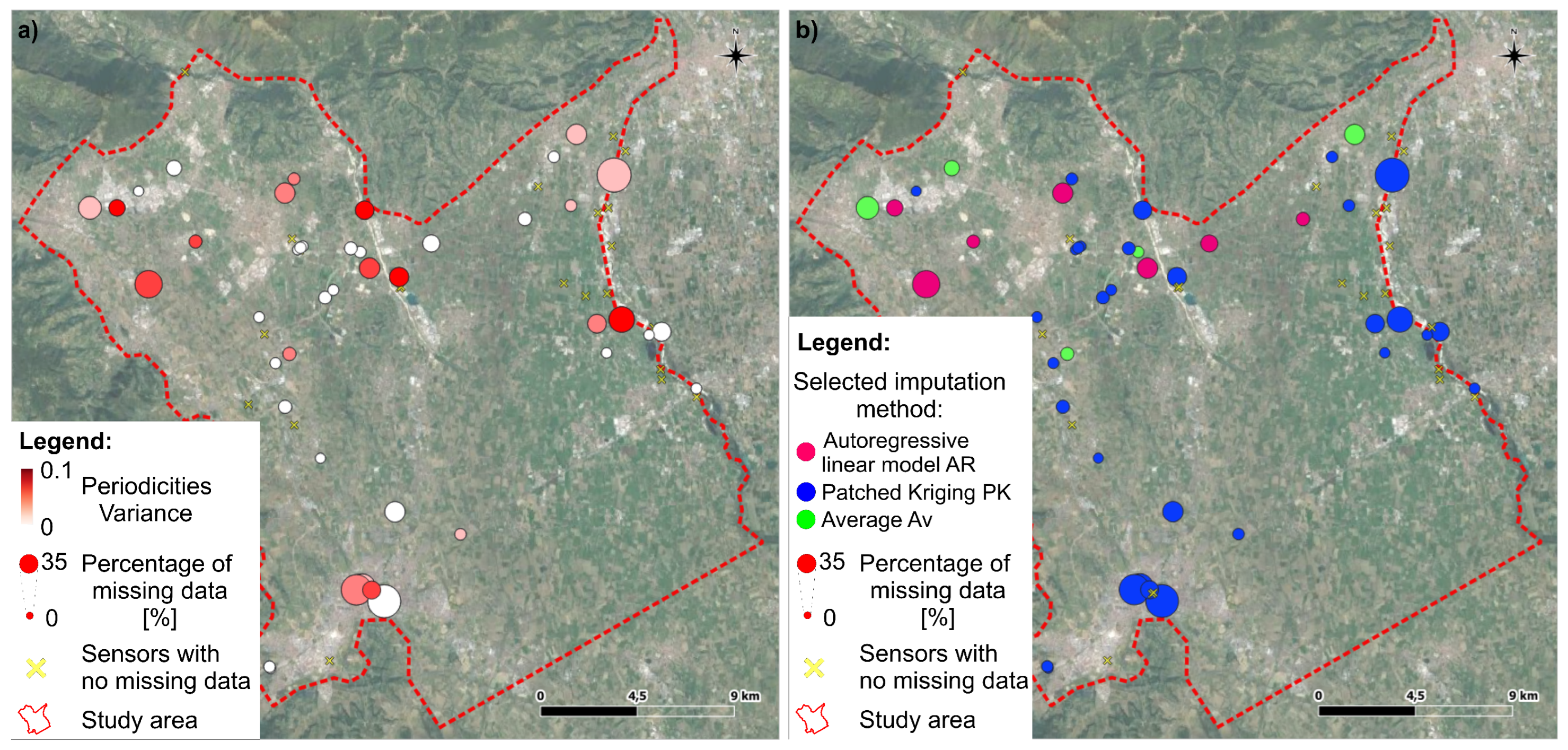
Figure 12.
(a) Map of the variability indicator for the Fourier Analysis and the periodicities variance. (b) Map of the prefered imputation method for each sensor (Cubic Spline CS, Autoregressive linear model AR, Patched Kriging PK, and their average). In both maps, the symbol dimension is related to the percentage of missing values in the recorded timeseries, and the yellow crosses represent the 26 timeseries without missing data.


Table 1.
Percentage daily errors of patched kriging interpolations differing on the applied range adjustment (RA): no RA, series RA, and interval RA for sensors 31, 37, and 57.
Table 1.
Percentage daily errors of patched kriging interpolations differing on the applied range adjustment (RA): no RA, series RA, and interval RA for sensors 31, 37, and 57.
| No RA | Series RA | Interval RA | |
|---|---|---|---|
| Sensor 31 | 5.00 | 4.76 | 11.71 |
| Sensor 37 | 165.08 | 11.12 | 19.52 |
| Sensor 57 | 13.76 | 12.24 | 16.34 |
Table 2.
Estimated R2 between the imputed timeseries, using the imputation methods (Cubic Spline CS, Autoregressive linear model AR, Patched Kriging PK, and their average) and the original recorded timeseries for each analyzed long timeseries. R2 estimated only for the interpolated intervals, roughly of the complete timeseries.
| Sensor 31 | Sensor 37 | Sensor 57 | |
|---|---|---|---|
| CS | 0.34 | 0.18 | 0.00 |
| AR | 0.69 | 0.40 | 0.08 |
| PK | 0.84 | 0.39 | 0.01 |
| Average | 0.80 | 0.48 | 0.07 |
Table 3.
Euclidean distances between the autocorrelation functions estimated from the timeseries interpolated by the imputation methods (Cubic Spline CS, Autoregressive linear model AR, Patched Kriging PK, and their average) and the autocorrelation function estimated from the original recorded timeseries.
| Sensor 31 | Sensor 37 | Sensor 57 | |
|---|---|---|---|
| CS | 0.0680 | 0.1420 | 0.1243 |
| AR | 0.0543 | 0.0783 | 0.0855 |
| PK | 0.0373 | 0.0359 | 0.0738 |
| Average | 0.0455 | 0.0503 | 0.0703 |
Table 4.
Five main periodicities (years), identified using each imputation method, observing the estimated power spectrum-sensor 92.
Table 4.
Five main periodicities (years), identified using each imputation method, observing the estimated power spectrum-sensor 92.
| 1st Peak | 2nd Peak | 3rd Peak | 4th Peak | 5th Peak | |
|---|---|---|---|---|---|
| CS | 0.42 | 7.17 | 0.80 | 1.19 | 1.79 |
| AR | 1.79 | 2.39 | 7.17 | 0.42 | 0.51 |
| PK | 1.79 | 2.39 | 7.17 | 0.42 | 0.51 |
| Average | 1.79 | 0.42 | 7.17 | 2.39 | 1.19 |
Table 5.
Five main standardized periodicities identified by each imputation method, observing the estimated power spectrum-sensor 92. For each power peak, the variances of the standardized periodicities of the four elaborated power spectra are reported in blue.
Table 5.
Five main standardized periodicities identified by each imputation method, observing the estimated power spectrum-sensor 92. For each power peak, the variances of the standardized periodicities of the four elaborated power spectra are reported in blue.
| 1st Peak | 2nd Peak | 3rd Peak | 4th Peak | 5th Peak | |
|---|---|---|---|---|---|
| CS | 0.06 | 1.00 | 0.11 | 0.17 | 0.25 |
| AR | 0.25 | 0.33 | 1.00 | 0.06 | 0.07 |
| PK | 0.25 | 0.33 | 1.00 | 0.06 | 0.07 |
| Average | 0.25 | 0.06 | 1.00 | 0.33 | 0.17 |
| 0.9 | 16.1 | 19.7 | 1.68 | 0.74 |
Table 6.
Calculations for the four microscale variability indicators referring to the maximum, minimum, mean, and overall range of the estimated microscale-sensor 92. For each indicator, the standard deviation , the mean , and the coefficient of variation are reported in blue.
Table 6.
Calculations for the four microscale variability indicators referring to the maximum, minimum, mean, and overall range of the estimated microscale-sensor 92. For each indicator, the standard deviation , the mean , and the coefficient of variation are reported in blue.
| Max | Min | Mean | Range | |
|---|---|---|---|---|
| CS | 11.31 | 6.67 | 8.65 | 4.64 |
| AR | 10.80 | 7.55 | 9.14 | 3.24 |
| PK | 11.02 | 7.55 | 9.26 | 3.46 |
| Average | 10.74 | 6.92 | 8.65 | 3.82 |
| 0.26 | 0.45 | 0.32 | 0.61 | |
| 10.97 | 7.17 | 8.92 | 3.79 | |
| 2.38 | 6.26 | 3.59 | 16.2 |
Disclaimer/Publisher’s Note: The statements, opinions and data contained in all publications are solely those of the individual author(s) and contributor(s) and not of MDPI and/or the editor(s). MDPI and/or the editor(s) disclaim responsibility for any injury to people or property resulting from any ideas, methods, instructions or products referred to in the content. |
© 2023 by the authors. Licensee MDPI, Basel, Switzerland. This article is an open access article distributed under the terms and conditions of the Creative Commons Attribution (CC BY) license (https://creativecommons.org/licenses/by/4.0/).
Share and Cite
MDPI and ACS Style
Meggiorin, M.; Passadore, G.; Bertoldo, S.; Sottani, A.; Rinaldo, A. Comparison of Three Imputation Methods for Groundwater Level Timeseries. Water 2023, 15, 801. https://doi.org/10.3390/w15040801
AMA Style
Meggiorin M, Passadore G, Bertoldo S, Sottani A, Rinaldo A. Comparison of Three Imputation Methods for Groundwater Level Timeseries. Water. 2023; 15(4):801. https://doi.org/10.3390/w15040801
Chicago/Turabian StyleMeggiorin, Mara, Giulia Passadore, Silvia Bertoldo, Andrea Sottani, and Andrea Rinaldo. 2023. "Comparison of Three Imputation Methods for Groundwater Level Timeseries" Water 15, no. 4: 801. https://doi.org/10.3390/w15040801
Note that from the first issue of 2016, this journal uses article numbers instead of page numbers. See further details here.