Assessing Climate Change Impact on Water Balance Components Using Integrated Groundwater–Surface Water Models (Case Study: Shazand Plain, Iran)

Abstract

Assessing the status of water resources is essential for long-term planning related to water and many other needs of a country. According to climate reports, climate change is on the rise in all parts of the world; however, this phenomenon will have more consequences in arid and semi-arid regions. The aim of this study is to evaluate the effects of climate change on groundwater, surface water, and their exchanges in Shazand plain in Iran, which has experienced a significant decline in streamflow and groundwater level in recent years. To address this issue, we propose the use of the integrated hydrological model MODFLOW-OWHM to simulate groundwater level, surface water routing, and their interactions; a climate model, NorESM, under scenario SSP2, for climate data prediction; and, finally, the HEC-HMS model to predict future river discharge. The results predict that, under future climate conditions, the river discharges at the hydrometric stations of the region may decrease by 58%, 63%, 75%, and 81%. The average groundwater level in 2060 may decrease significantly by 15.1 m compared to 2010. The results of this study reveal the likely destructive effects of climate change on water resources in this region and highlight the need for sustainable management methods to mitigate these future effects.

1. Introduction

One of the most complex challenges of the 21st century is global warming. Climate model simulations indicate drastic atmospheric temperature increases all over the world [1]. Recent climate changes have already had widespread effects on human and natural systems [2]. Climate change will pose short- to long-term risks to natural systems, including water resources. In some areas, the sustainable quantity of groundwater is threatened. Changes in streamflow, timing, and associated extremes are predicted to have a negative impact on freshwater ecosystems in many watersheds in the mid-to-long term in all studied scenarios [3]. Since groundwater resources are in direct interaction with surface water, the development and exploitation of each will have an impact on the other. Thus, integrated water resource management is required for future water security [4].

This requires understanding of complicated, linked groundwater and surface water processes [5]. In the past decades, several studies have assessed the impact of climate change on surface water [6,7,8,9] and groundwater separately [10,11,12,13]. Over time, some coupled or integrated models were introduced that analyzed surface water–groundwater interactions, which provided the possibility of analyzing joint flow systems. Some of these coupled models were used in different studies to quantitatively assess the effects of climate change on surface water and groundwater exchange, like the coupled SWAT-MODFLOW [14,15], Mike-SHE [16], and GSFLOW [17]. Another integrated hydrological flow model that can assess surface-water/groundwater interactions is the MODFLOW One Water Hydrologic Flow Model (MF-OWHM), which is the most complete model to date to analyze the integrated use of groundwater and surface water [18]. The MF-OWHM has successfully been applied in the Colorado River delta, Mexico, to improve understanding of the dynamics of surface–groundwater interactions in the Delta aquifers [19]. It has also helped to understand recharge and flow processes and proper water management in the Hout Catchment, Limpopo Province, South Africa [20]. Ref. [21] used MF-OWHM to simulate large-scale surface and groundwater budgets for the United States. The model can also be used to study the response of the hydrological system under different future climate scenarios. Azeref et al. used MF-OWHM in Ethiopia under two scenarios (changes in withdrawal and recharge) to evaluate changes that might occur in groundwater and river leakage [22]. Another capability of MF-OWHM is to link land subsidence/uplift with deformation-dependent flows and indirect effects on conjunctive groundwater–surface water use [23]. However, none of these modeling studies used MF-OWHM to simulate groundwater–surface water interaction in response to climate change.

According to the IPCC, the possible effects of climate change on the quantity and quality of water resources are more severe in arid and semi-arid regions as compared to other parts of the world [24]. Most of Iran is located in arid and semi-arid areas, and the limited annual rainfall is already resulting in severe water scarcity. Thus, future climate change is likely to aggravate the situation. Streamflow reduction, groundwater level decline, loss of more than 405 aquifers, soil salinization, land subsidence, and dust storms are the most obvious effects of climate change and water supply overuse in this country during recent years. Dwindling surface water has caused irreparable damage to most aquifers in the country in the past decades [25]. Overexploitation of groundwater has resulted in water level drops and reduced the quality of aquifer water [26]. According to the latest report of the Information Technology and Statistics Office of the Ministry of Energy of Iran, about 43% of the country’s water needs are supplied from surface water resources and 57% from groundwater. In this situation, when both surface water and groundwater resources contribute to the needs of all sectors and the country is undergoing severe climate change, quantifying the availability of water under current and future conditions is a vital aspect of the evaluation and planning of water management policies.

Optimal use of water resources, especially groundwater, plays a key role in Iran’s economic development. The central watersheds of Iran have less rainfall than other parts of the country and, consequently, the amount of renewable groundwater in these areas does not suffice for existing withdrawal. In general, the increase in population and the expansion of industrial and agricultural activities without consideration of the natural potential of the region have led to an increase in water requirements for drinking, health and recreation, and industrial activities. On the other hand, the occurrence of recent consecutive droughts, reductions in surface water resources, a greater tendency to use groundwater resources, poorly integrated management in the water sector, and many other factors in the centrally located Shazand Plain have resulted in restrictions on groundwater use on the entire plain since 1991 [27]. However, continuing the current trend may lead to irreparable damage to the groundwater resources of this region.

In general, this study’s objectives are:

• Evaluating the feasibility of using MF-OWHM and HEC-HMS for simulating the groundwater level and river discharge in the study area;
• Improving the understanding of the area´s river and groundwater interaction;
• Evaluating future rainfall and temperature patterns;
• Prediction of river discharge and groundwater levels under climate change.

2. Materials and Methods

2.1. Study Area

The Shazand Plain area is located in the Qarachai watershed in the southwest of Markazi Province in Iran, with an area of 984 sq. km. Figure 1 shows the location of the Shazand Aquifer. It lies between the north latitudes of 33°43′ to 34°11′ and east longitudes of 49°16′ to 49°52′. According to the Geiger–Koppen classification, Shazand’s climate is continental (Dsa). It has warm summers and cold winters due to its mountainous area and elevation of 1920 m above mean sea level. Shazand is one of the coldest regions of Markazi Province. Its mean annual temperature is about 12.4 °C. The daily temperature of the region can reach 33 °C in summer and −25 °C in winter. Due to the location of the Shazand area on the eastern slopes of the Zagros Mountains, most of its precipitation forms due to moist air masses that come from the west, northwest, and southwest [28]. The long-term mean annual precipitation and potential evapotranspiration in Shazand plain are 338 and 2750 mm per year, respectively. There is a rain gauge station to the west and an evaporation station to the east of the study area. According to the Iran Meteorological Organization, precipitation in the west of the region is higher than in the east.

Water Resources in Shazand

Gharechai River is one of the most important rivers in central Iran. Shazand forms the tributary of this river. The Cheshme-Emarat River flows from the south, and the Azna River from the west, Mohajeran River from the northeast, and Tore River from the northwest join it during its course through the plain [29]. Data from four hydrometric stations were used in this study (Figure 2). The discharge at these stations shows a decrease of about 35% to 60% during the last 5- to 7-year period compared with the mean of the 30-year period. This indicates a significant decline in the surface water of the region [27].

In 1998, 17 piezometric wells were installed in the region to observe groundwater level changes. Groundwater exploitation includes 1143 wells with an annual discharge of about 185 million cubic meters (MCM). Water consumption in this area includes 192 MCM per year of groundwater (wells and aqueducts), which is used for agriculture, drinking, and industry [27]. The water balance data for the Shazand area are presented in

Table 1. Water balance data for the Shazand area.

MCM	Agriculture	Industry	Drinking	Total
Groundwater Discharge	231.11	8.82	13.58	283.51
Surface Water Discharge	5.87	-	-	5.87
Total Discharge	236.98	8.82	13.58	289.32
Return Flow from Groundwater	79.11	6.21	6.86	92.18
Return Flow from Surface Water	1.76	-	-	1.76
Total Return Flow	80.88	6.21	6.86	93.95
Net Groundwater Consumption	151.87	2.61	6.72	161.20
Net Surface Water Consumption	4.11	-	-	4.11
Total Net Consumption	155.98	2.61	6.72	165.31

. Consequently, groundwater levels are continuously decreasing in the Shazand Aquifer, from west to east.

2.2. Methodology

To improve water resource management and prevent further damage to water resources in the Shazand Plain, improved knowledge of surface water and groundwater interaction under future climate conditions is necessary. For this reason, the MF-OWHM was applied to the area using the CHD, WEL, RCH, and SFR packages. The model was calibrated and validated by trial and error. The Norwegian Earth System Model version 2 (NorESM2) under the SSP2 scenario was then used to simulate the future climate. Downscaling was performed to adjust gridded precipitation and temperature data to the catchment area. HEC-HMS was then set up, calibrated, and validated to simulate river discharge. The verified model was used for prediction of river discharge under future climate scenarios. Finally, interactions between river water and groundwater were analyzed using MF-OWHM. Figure 2 presents a brief summary of the methodology in this study.

2.3. Model Development and Input Data

2.3.1. MODFLOW-OWHM

The MODFLOW One-Water Hydrologic Flow Model (MF-OWHM) is an integrated hydrological model based on MODFLOW-2005 that can simulate and analyze different environmental conditions. The term “integrated” refers to the connection of groundwater, surface water, aquifer compaction, and subsidence [18]. In MF-OWHM, the hydraulic head is calculated by summing a pressure term, an elevation term, and a kinetic energy term. Because of nonmoving or slowly moving bodies of water, the kinetic energy term can be assumed to be zero. The hydraulic head equation can then be simplified to:

$$h=\frac{P}{\rho g}+Z$$

(1)

where h is the hydraulic head, P is the gauge pressure measured at elevation Z, $\rho$ is the freshwater density, g is the acceleration due to gravity, and Z is the elevation that the gauge pressure is measured at.

In MF-OWHM, groundwater flows according to the changes in the hydraulic head, like in MODFLOW. Groundwater flows to regions of the aquifer that have a lower hydraulic head according to Darcy’s law and the conservation of mass (continuity) equation.

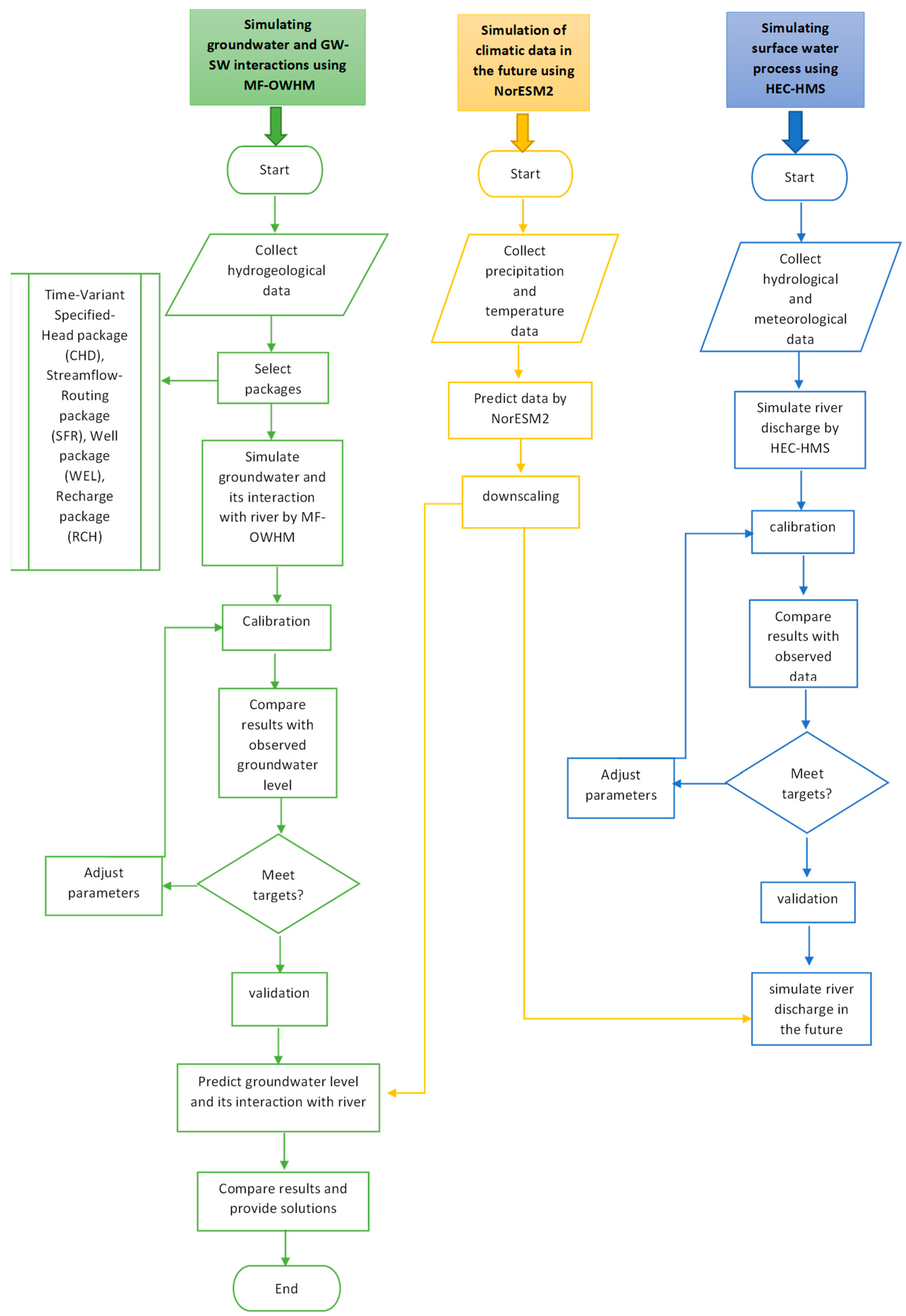
MF-OWHM consists of different packages for multiple purposes that were used in this study: the Time-Variant Specified-Head package (CHD) was used to simulate specified head boundaries, the Recharge package (RCH) was used to simulate a specified flux from precipitation infiltration distributed over the top of the model, the Well package (WEL) was used for simulating a specified flux to individual cells, and the Streamflow-Routing package (SFR) was used for simulation of streams and their interactions with groundwater. The ModelMuse software used in this study is a graphical user interface (GUI) for U.S. Geological Survey models like MODFLOW6, MODFLOW-2005, MODFLOW-NWT, and MODFLOW-OWHM [30].

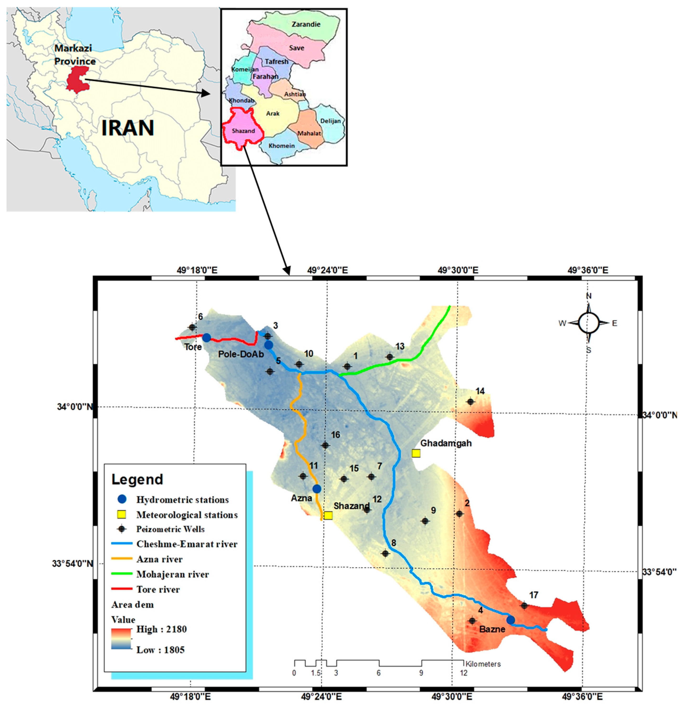
The Shazand Aquifer was divided into 7316 cells with a size of 300 m × 300 m. To ensure good model performance and analyze river and groundwater interactions, the aquifer was simulated with one year (2009–2010) of data and 12 one-month stress periods consisting of one steady state and the rest transient stages. Precipitation and evaporation data from two climate stations were used to calculate the recharge from rainfall infiltration. Inside the catchment, there are 32 wells for domestic purposes, 35 wells for industrial use, and 756 wells for agricultural use, and their pumping rates were added to the WEL package. It should be noted that, because the groundwater level is 5 m below the ground surface, groundwater evaporation does not take place in this area. Thus, the evaporation package was not used.

• Streamflow routing and its interaction with groundwater

The SFR package calculates water exchange between river channels and groundwater and routes of river discharge downstream [21]. When the groundwater level is lower than the surface water, water drains into the groundwater. When the groundwater level is above the surface water system, water discharges from groundwater to the surface water. These exchanges create a dynamic link between surface water and groundwater systems that is simulated [18]. In MF-OWHM, the rainfall–runoff process is considered for a conjunctive use. Surface water flow is routed through distribution of precipitation, excess water from irrigation, surface water diversions and deliveries, subsurface flows, and groundwater that discharges to surface water. The streamflow routing process is represented as a head-dependent package in MF-OWHM. The flow is always in the direction of the canals, and the recharge and discharge to the aquifer are assumed to be constant at each time step [18]. Flow between streams and aquifers in this package is calculated using Darcy’s law and assuming uniform flow between a stream and an aquifer in a section of the stream and the corresponding volume of the aquifer [18]. The flow is computed as:

$$Q_L=\frac{K_{sb} w L}{m} \left(h_s-h_a\right)$$

(2)

where Q_L is the flow between a section of the stream and the aquifer, K_sb is the hydraulic conductivity of the streambed, w is the width of the stream, L is the length of the stream, m is the thickness of the streambed, h_s is the stream head, which is computed by adding the stream depth to the elevation of the streambed, and h_a is the aquifer hydraulic head beneath the streambed.

In Equation (2), leakage from the streambed to the aquifer can change depending on the aquifer head and the stream. The flow that seeps from the stream bed to the aquifer is calculated by multiplying the wetted area of the stream by the infiltration rate. The wetted area can be constant or specified based on the stream’s cross-sectional dimensions, discharge, and stage. Manning’s equation is used for calculating the relation between stage and discharge.

The SFR package routes streamflow via a network of channels that are divided into reaches and segments. A reach is a part of a river that is linked to a particular finite-difference cell to model groundwater flow and a segment is a group of reaches that have common characteristics such as uniform precipitation over them, uniform evaporation from them, and uniform changing properties, such as streambed elevation, hydraulic conductivity, streambed thickness, and stream depth and width. A stream water budget and leakage rate are calculated for each reach at the end of each time step and separated from the groundwater flow budget. This water budget determines the amount of water that is available to leak from the stream into the aquifer. The package uses the volumetric continuity equation so that the sum of flows into the reach $\sum Q_{in}$ is equal to the sum of flows out of the reach $\sum Q_{out}$:

$$\sum Q_{in}=\sum Q_{out}$$

(3)

The package includes several sources of inflow to a reach:

$$\sum Q_{in}=Q_{sri}+Q_{trb}+Q_{ppt}-Q_{li}$$

(4)

where $Q_{sri}$ is the specified inflow at the beginning of the first reach, $Q_{trb}$ is the sum of tributary flow from upstream into a reach, $Q_{ppt}$ is direct precipitation over a reach, and $Q_{li}$ is groundwater leakage to a reach.

The package also allows several losses from a stream reach, including:

$$\sum Q_{out}=Q_{sro}+Q_{div}+Q_{et}+Q_{lo}$$

(5)

where $Q_{sro}$ is the streamflow out of a reach $Q_{div}$ is a specified diversion from the last reach, $Q_{et}$ is evaporation from a reach, and $Q_{lo}$ is leakage into the aquifer.

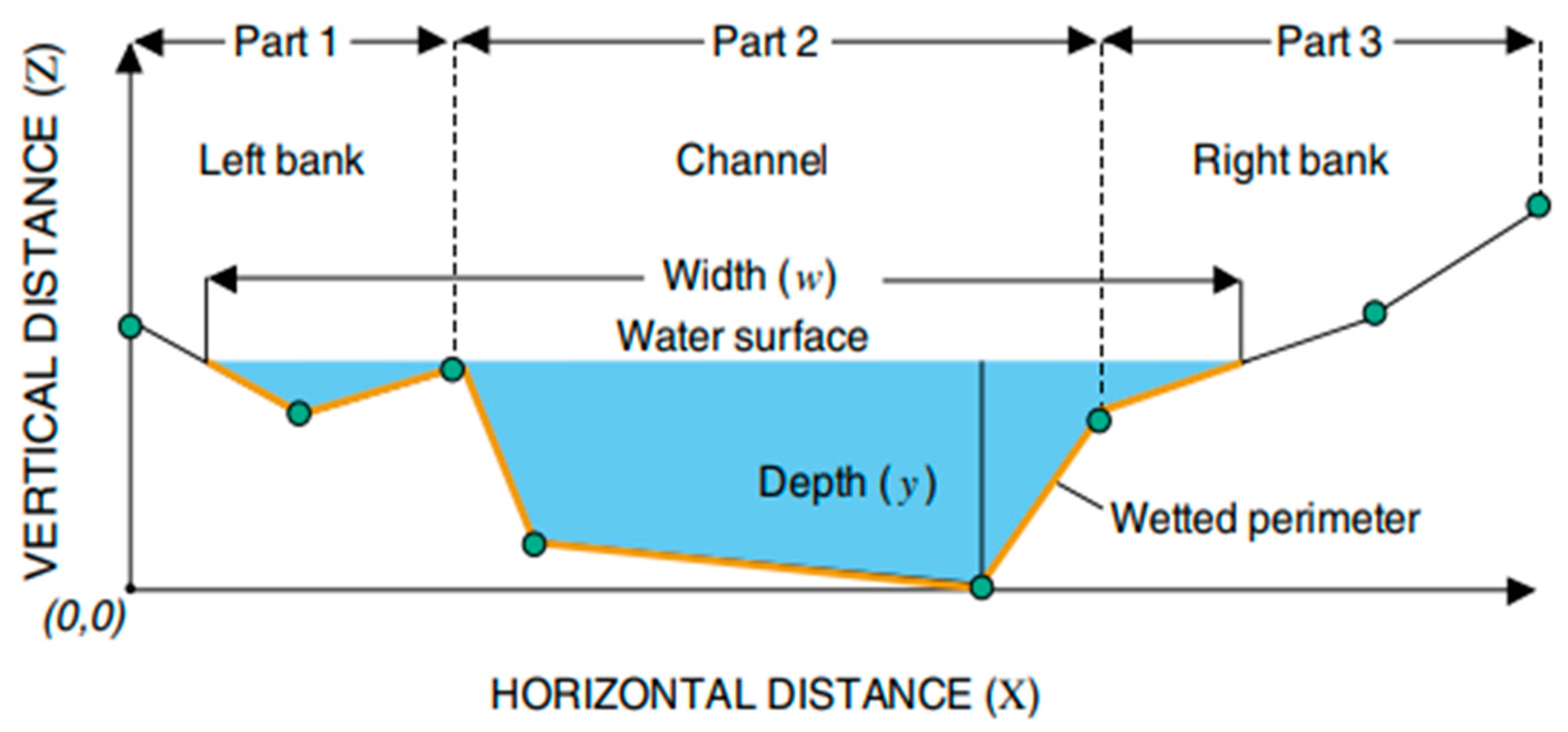
There are five options to compute stream depth in this package. The option selected uses Manning’s equation, but the channel is divided into an eight-point cross-section (Figure 3). Depth (y) is calculated by computing the flow for an estimated depth until the time that the difference between the computed flow $\left(Q_n\right)$ and the streamflow at the midpoint point of the reach becomes very small. The simple form of the equation is defined as:

$$y_n=f\left(y_{n-1}\right)\frac{f\left(y_{n-1}\right)\left(y_{n-1}-y_{n-2}\right)}{f\left(y_{n-1}\right)-f\left(y_{n-2}\right)}$$

(6)

where n is the iteration number;$f\left(y_{n-1}\right)$ is $Q_{n-1}-Q_{mdpt}$ for depth $y_{n-1}$; and $f\left(y_{n-2}\right)$ is $Q_{n-2}-Q_{mdpt}$ for depth $y_{n-2}$

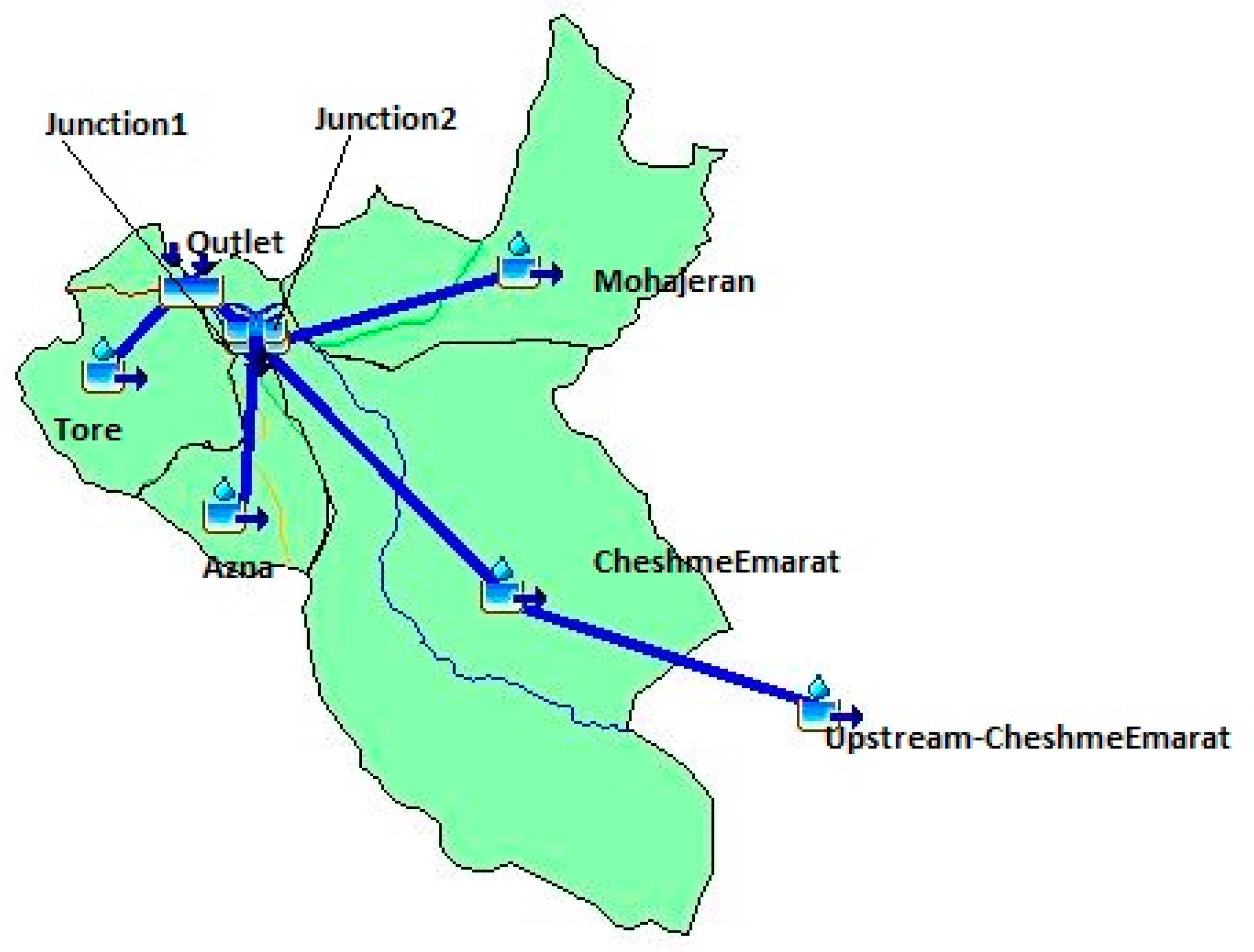
The four main rivers were considered as four segments, each of which was divided into smaller parts called reaches [18]. For the flow parameter in this package, hydrometric station data were used, and, when a hydrometric station was not available in a segment, data were obtained from other hydrometric stations by using the discharge-area ratio method. To simplify calculations in the SFR package, the riverbed thickness was set to 1 m and channel roughness was set equal for all river segments.

2.3.2. HEC-HMS

The HEC-HMS model was used to simulate future river discharge by using downscaled climate data. The output of the HECHMS model was used in the MF-OWHM model to simulate future river and aquifer interaction. The HEC-HMS, developed by the US Army Corps of Engineers Hydrologic Engineering Center, is capable of modeling both continuous and event-based runoff [18]. HEC-HMS consists of four components including a basin component, meteorological component, control specification, and input data component. The model uses different methods to transform rainfall into runoff, including the Clark unit hydrograph, SCS unit hydrograph, ModClark, and kinematic wave. The model consists of different methods for computing loss, among which soil moisture accounting (SMA) is a continuous method used for longer periods [31]. The SMA method uses five storage layers to represent the watershed. The layers include canopy interception, surface depression storage, soil, upper groundwater, and deeper groundwater involving twelve parameters (Figure 4).

To simulate river discharge in the HECHMS model, the Shazand study area was divided into five sub-basins consisting of two junctions and one outlet (Figure 5). The Clark unit hydrograph method was used to transform rainfall to runoff. The soil moisture accounting (SMA) method was used for loss and the constant monthly method for baseflow. Moreover, daily rainfall data were obtained from two stations (Shazand and Ghadamgah) and daily temperature was collected from the Ghadamgah evaporation station. The evapotranspiration values were computed based on the Hamon method.

2.3.3. NorESM2

The Norwegian Earth System Model version 2 (NorESM2) is the second generation of the coupled Earth system model (ESM) developed by the Norwegian Climate Center and is the successor of NorESM1 [33]. In NorESM2, a new natural DIC tracer, which simulates changes in the natural DIC components, was introduced [34]. Currently, NorESM2 is available in three versions: NorEsm2-LM, NorEsm2-MM, and NorEsm2-LME. The first two versions share the same horizontal resolution of 1° for the ocean and sea-ice components, but they differ in the horizontal resolution of the atmosphere and land components [34]. The third version can be applied in interactive carbon-cycle programs but is the same as NorESM-LM in all other parts. SSP_s scenarios are used as important inputs for the latest climate models, feeding into the sixth assessment report of the Intergovernmental Panel on Climate Change (IPCC). These scenarios regard five distinct ways in which the world might change in the absence of climate policy and how different levels of climate change mitigation could be achieved when the mitigation goals of RCPs are combined with the SSPs. SSP2, which is called the “middle of the road” is one of those scenarios in which development and income growth do not proceed evenly, and there is a decline in the consumption of energy and resources.

One of the problems with using climatic model outputs is the large temporal and spatial scale of the computed cells compared to the study area [35]. There are different methods to produce regional climate scenarios from simulation climate models, which are called downscaling [36]. MRQNBC is a statistical downscaling method that can be used alongside the NorESM model.

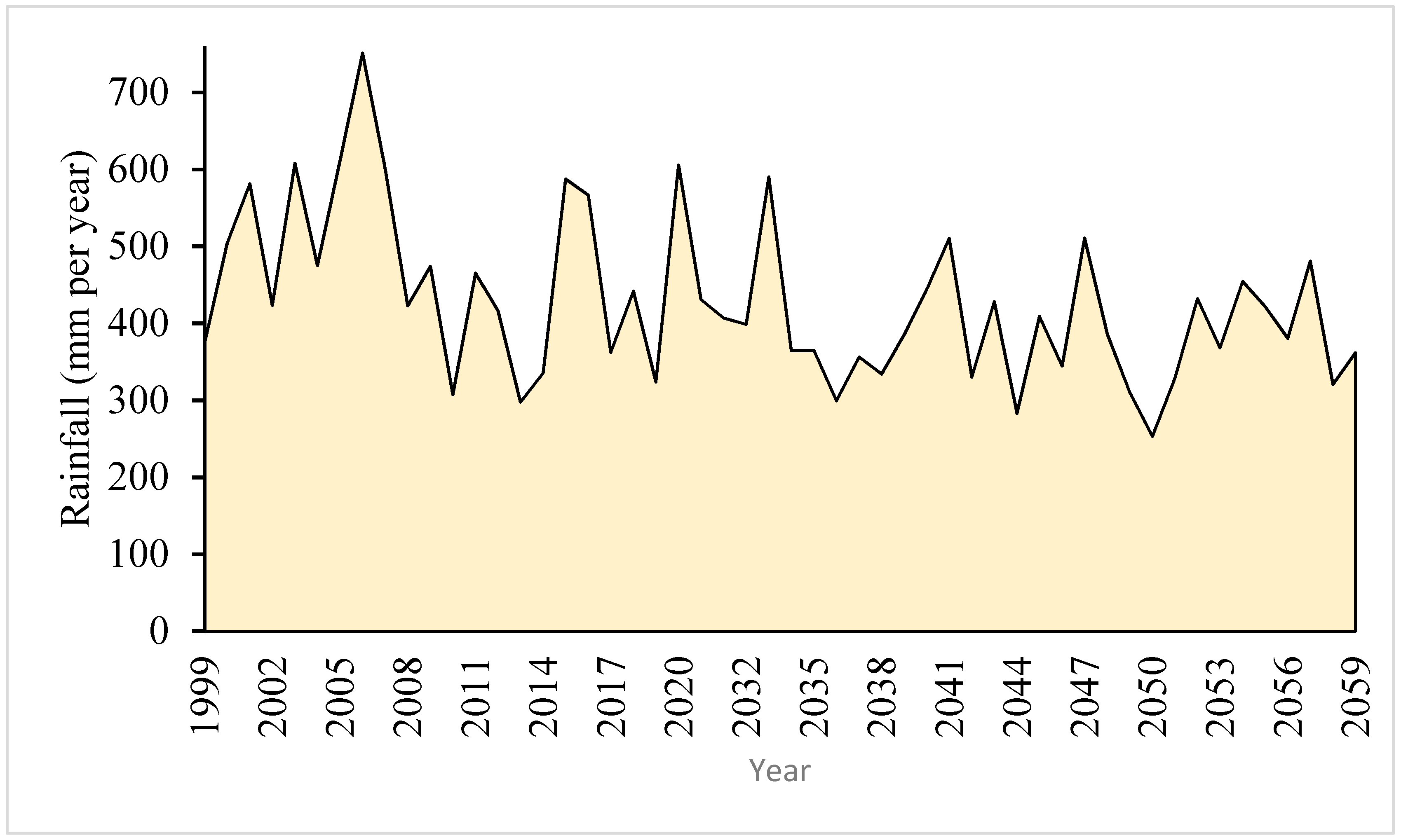
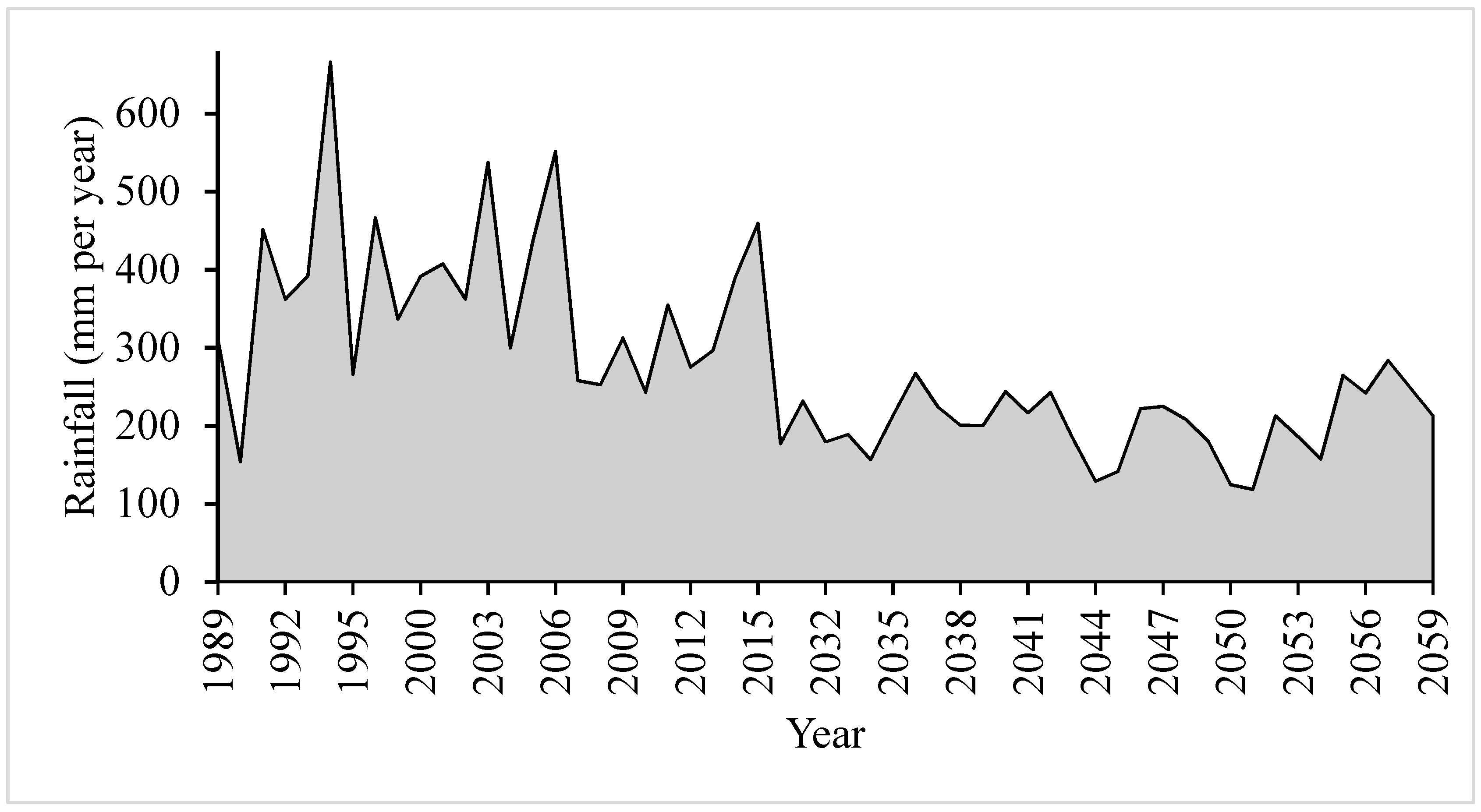
NorESM2-LM, under one of the shared socioeconomic pathway scenarios (SSP2) from the Scenario Model Intercomparison Project defined under CMIP6 [37], was used to predict future climate data. For this purpose, daily rainfall data from the Ghadmagah station during 1984–2015 and the Shazand station during 1999–2020 and average daily temperature data from the Ghadamgah station during 2003–2020 were used. Data from NorESM2 were downscaled by the MRQNBC method to generate regional daily climate data that was used as an input to the HEC-HMS and MF-OWHM models.

3. Results

3.1. MODFLOW-OWHM

The hydrological model for Shazand Basin was calibrated for 2009–2010 and validated for 2010–2011 in two steps. First, by using riverbed hydraulic conductivity, the observational river discharge data at the Pole-DoAb station (Figure 1) were used in comparison to river flow, which was routed in the SFR package. Each river segment was divided into upstream and downstream parts, and their hydraulic conductivity was estimated by trial and error (

Table 2. Riverbed hydraulic conductivity.

River Segment	Upstream Hydraulic Conductivity (m/day)	Downstream Hydraulic Conductivity (m/day)
Cheshme-Emarat	1.3	1.9
Azna	1.1	1.4
Mohajeran	1.8	1.8
Tore	3.0	1.1

).

According to the results, the lowest hydraulic conductivity of the riverbed was in the downstream Azna segment (1.1 m/day). The highest riverbed hydraulic conductivity was in the downstream Tore segment (3 m/day). Figure 6 shows the observed and routed river flow at the Pole-DoAb hydrometric station, which has the highest river discharge in the region.

According to the calculated error metrics, the SFR package’s capability of routing river flow is good (

Table 3. Error metrics for streamflow routing in MF-OWHM.

Error Metric	Value
R2	0.97
MAPE	0.21
RMSE (m3/s)	0.126

).

In the next step, the aquifer’s hydraulic conductivity was calibrated by comparing observed and simulated groundwater levels in 17 piezometers. For this purpose, the area was divided into different zones and the hydraulic conductivity of each zone was estimated by trial and error. The hydraulic conductivity varied from 3 to 55 m/day, with the highest values in the middle of the aquifer and the lowest in the northwest of the aquifer (Figure 7). The minimum groundwater level is associated with the piezometers in the east of the region and the piezometers in the northwest have the highest groundwater level in the region.

R² and RMSE were 0.99 and 1.67 m, respectively, for the simulated and observed groundwater levels for 17 piezometers in the steady state, indicating the acceptable performance of the model.

Table 4. RMSE values for piezometers in the transient state.

Piezometer Name	RMSE (m)	Piezometer Name	RMSE (m)
N1	2.15	N10	1.10
N2	1.22	N11	0.75
N3	2.70	N12	2.17
N4	0.79	N13	2.68
N5	1.21	N14	1.51
N6	1.45	N15	1.95
N7	2.54	N16	1.91
N8	1.33	N17	2.69
N9	2.20

shows the RMSE for 17 piezometers in the transient state and good performance of the model in this case as well. R² and RMSE were 0.997 and 1.98 m, respectively, which indicate acceptable errors (Figure 8).

Water Budget and River–Aquifer Interaction

The annual simulation results showed that infiltration from the river makes the lowest contribution to aquifer recharge in all months of the year. During the autumn, winter (except March), and spring, the constant head contributed the largest share to aquifer recharge, while during the summer and March, infiltration from rainfall had a greater share than the constant head in aquifer recharge. Regarding aquifer discharge, during the summer and October, well extraction had the largest share, while in autumn (except October), winter and spring, the constant head had a larger share than well extraction in (

Table 5. Water budget simulation results.

Month	Constant Head (In) (%)	Rainfall Infiltration (%)	River Leakage to Aquifer (%)	Constant Head (Out) (%)	Well Withdrawal (%)	Aquifer Leakage to River (%)
October	83	8.0	1.3	13	79.5	0.9
November	62	29	1.3	55	41	1.1
December	66	19	1.3	56	42	0.9
January	68	25	1.6	87	9.0	1.4
February	61	34	2.1	87	7.0	1.8
March	31	62	4.1	88	4.0	3.0
April	23	68	7.3	88	5.5	4.2
May	28	66	4.6	88	5.5	4.6
Jun	82	9.0	3.3	71	25.5	2.7
July	87	3.0	1.5	38	59	1.3
August	89	0.0	1.3	31	67.5	1.0
September	89	0.0	0.9	28	69.5	0.6

).

In all months, the amount of water infiltrated from the river to the aquifer was greater than the amount of water discharged from the aquifer to the river. Most of the infiltration from the river to the aquifer occurred in the Tore segment in the northwest of the region and in the downstream of the Cheshme-Emarat segment in the north.

3.2. HEC-HMS Results

The rainfall–runoff model was calibrated for 2009–2013 and validated for 2013–2014. For this purpose, the observed river discharge at each station was used to compare to the simulated discharge at each station. Automatic model calibration was used to calibrate the Clark unit hydrograph parameters, SMA parameters, and other model parameters such as Muskingum k and x, aiming to maximize the Nash–Sutcliffe and coefficient of determination.

Figure 9 and Figure 10 show observed and simulated river discharge for the Pole-Do-Ab hydrometric station, which is located near the watershed outlet, for calibration and validation. Calculated error metrics for calibration and validation show that the capability of the model for simulating river discharge in the Shazand watershed is acceptable (

Table 6. Error metrics for the HEC-HMS calibration.

Station	R2	Nash Sutcliffe	RMSE (m3/s)
Pole-Do-Ab	0.72	0.69	0.35
Tore	0.77	0.77	0.10
Azna	0.63	0.62	0.17
Bazne	0.40	0.56	0.03

and

Table 7. Error metrics for the HEC-HMS validation.

Station	R2	Nash Sutcliffe	RMSE (m3/s)
Pole-Do-Ab	0.76	0.65	0.23
Tore	0.63	0.40	0.02
Azna	0.78	0.54	0.03
Bazne	0.59	0.38	0.08

).

3.3. Future Scenario Predictions

3.3.1. Climate Projection

The climatic model (NorESM2-LM) was used to generate daily rainfall (Shazand and Ghadmagah stations) and daily temperature (Shazand station) for the 30-year period (2030–2059). These data were downscaled using the MRQNBC.

Comparing the historical long-term annual data with the future data at the Shazand station shows that the rainfall may decrease from 479 to 389 mm per year with a decrease of 18% (Figure 11).

For the Ghadmagah station, the rainfall may decrease from 369 to 202 mm per year (−45%) (Figure 12), and average daily temperature at this station will probably increase by 16% from 13.7 to 15.9 °C (Figure 13). According to these results, the east of the region, which had less rainfall in the past, will have a more severe decrease in rainfall in the future compared to the west of the region.

3.3.2. Climate Change Impacts on Surface Water

The HECHMS model was used to predict the stream flow using the downscaled climatic data for the period 2030 to 2059. Comparison of the historical long-term annual discharge with the future values showed that the largest decrease may occur at the Bazneh station, by 81%, and the smallest decrease may occur at Tore station, by 58%. The river discharge reductions at the Azna and Pole-Do-Ab stations were 63% and 75%, respectively (Figure 14).

3.3.3. Climate Change Impacts on Groundwater

The groundwater level was predicted using MF-OWHM for the period 2030–2059 at monthly time steps. Figure 15 shows the drop in piezometer levels from 2010 to 2059. Piezometer N13, in the northeast of the region, may have the largest decrease, with a drop of about 33 m. In general, under the future climate, the east and northeast parts of the region will probably face larger decreases in groundwater level. The minimum groundwater decrease may occur in the northwest of the region, which is in line with climate model predictions that shows more decline in rainfall in the eastern area. The overall aquifer water level in 2059 is predicted to be about 1857 m, which means that the water level may decrease by 15 m compared to the groundwater level in 2010.

3.3.4. Climate Change Impacts on Water Budgets and River–Aquifer Interaction

Table 8. Average volumetric water budgets for an average of 30 years (2030–2059) compared to baseline (2010).

In	Future (MCM)	Baseline (MCM)	Changes from Baseline (MCM)	Out	Future (MCM)	Baseline (MCM)	Changes from Baseline (MCM)
Storage	12.81	20.35	−7.54	Storage	26.69	76.06	−49.37
Constant head	62.9	113.03	−48.13	Constant head	53.13	85.95	−32.8
Precipitation infiltration	68.69	101.06	−32.37	Well extraction	85.2	85.2	0
Stream leakage	7.70	18.65	−13.95	Stream leakage	5.04	12.6	−7.02
Total	152.10	253.09	−100.99	Total out	165.06	259.81	−94.75

presents a comparison of the water budget components for an average of 30 years compared to the baseline year, 2010. According to the water budget results, the total amount of groundwater will decrease in the coming years. According to the table, infiltration from the river will contribute the lowest share to aquifer recharge. Well extraction and constant head will play the biggest roles in aquifer discharge.

The results show that the volume of water exchanged between the aquifer and river will decrease due to the decrease in the total volume of water, and this is more evident in the amount of water transferred from the aquifer to the river because the groundwater level will drop significantly. This downward trend will continue throughout the forecast years. According to the SFR package’s forecast results, the highest infiltration from the river to the aquifer in most months of the simulation will occur in the downstream of the Cheshmeh-Emarat segment, in the north of the region, and the lowest river infiltration will occur in the Azna segment, in the west of the region.

4. Discussion

MODFLOW-OWHM, an integrated hydrological model, and HEC-HMS, a rainfall–runoff model, have been used to study the status of water resources in the Shazand plain, Iran under climate scenarios. The NorESM2 model was used to predict climate data under the SSP2 scenario. This study was adopted to simulate streamflow, groundwater level, and surface water–groundwater exchanges under climate change scenarios. Both surface water and groundwater in the Shazand area are greatly affected by climate change. The interaction between surface water and groundwater in this region is not that strong that they can affect each other greatly. It can be concluded that the significant reduction in streamflow in recent years in Shazand was caused by climate change, not by groundwater level decline. The decrease in rainfall will be more in the east of the region, and, because of this, water resources in the east of the area will be severely affected in the future. From the mentioned simulation results, it can be seen that the MF-OWHM model has good applicability in simulating groundwater and surface water–groundwater exchanges and routing streamflow.

Studies show that the ever-increasing demand for water in most regions is met by both surface water and groundwater, so choosing an appropriate model to investigate the exchanges between the two systems is very important, because the demands placed on one have direct effects on the other. The previous studies have mostly examined each of the systems separately and ignored the effects of the two on each other. Some studies have examined groundwater–surface water exchanges using the SWAT-MODFLOW model. It is important to consider that this model is not capable of simulating the two systems’ interactions in as much detail as MF-OWHM does. In this paper, MF-OWHM was adopted to assess the statuses of surface water, groundwater, and their interactions under climate change scenarios in the study area. Although MF-OWHM is good at simulating groundwater and its interactions with surface water, it does not include the watershed rainfall–runoff process, so using a rainfall–runoff model is necessary for predicting the river discharge in the future.

Models are undoubtedly subject to uncertainty because of their simplification of reality [38]. Uncertainties in studies related to climate change’s impact on water resources arise from the climate model projection, downscaling, and the hydrological models [39]. The uncertainties in the outputs of hydrological models originate from three sources of errors: input data, model structure, and model parameters [40]. In this study, there are uncertainties in parameters such as estimated hydraulic conductivity, pumping observations, boundary conditions, streambed thickness, and streambed elevation. Uncertainties in these parameters misrepresent the aquifer [21]. For example, a wrong estimation of riverbed hydraulic conductivity leads to wrong simulation of groundwater and river interactions. Among all sources of uncertainty, uncertainty in parameters is easier to control through calibration procedures [41]. In this study, calibration was carried out by trial and error in order to adjust parameters. The simulated results of the applied models show a good correlation with observed data.

In this study, water demand was not simulated. Further studies could link population increase with landscape, groundwater, and surface water processes. This could combine water loss from irrigation, imported water, rainfall, and evaporation to groundwater and surface water [18]. Scenarios such as increasing well extraction or decreasing rainfall infiltration can also be used to assess impacts on aquifers and river exchanges [22]. Combined optimization can be used with this scenario to better manage future water resources [22,42]. The use of other available models for the integrated modeling of surface water and groundwater and the comparison of their results with this study is also suggested.

5. Conclusions

Investigation of surface water and groundwater statuses and their interaction helps decision-makers to make effective decisions for the sustainable management of water resources [43]. The purpose of this study was to investigate the impacts of climate change on surface and groundwater resources and their exchanges by modeling the Shazand Basin and aquifer. For this purpose, the new MODFLOW-OWHM model was used to simulate groundwater and its interaction with surface water, and the rainfall–runoff model HEC-HMS was used to simulate surface water flow. The climatic model NorESM2, under the scenario SSP2 and using the downscaling method MRQNBC, was used to predict the future meteorological state. The downscaled climate results were then used to predict surface water flow with the HEC-HMS model. The results of this model were used to predict future groundwater and its interaction with surface water. The major findings of this research are:

• Rainfall in the region will decrease by 18–45% (2059). The results indicate that the eastern region will experience a stronger rainfall decline.
• Average annual temperature is projected to rise in the region by the end of 2059 by 16% (from 13.7 to 15.9).
• Under the climate change scenarios, river discharge will decrease by 63–81% by the end of 2059. The smallest reduction may be expected at the Tore runoff station in the western region.
• By the end of 2059, the groundwater level of the region may drop significantly (maximum of −33 m). The northeastern region will probably be most affected, while the northwestern region will face less decline in groundwater level.
• Under the climate change scenario, when the streamflow and groundwater level are declining, the volume of water exchanged between the aquifer and the river will also decrease.
• The highest stream leakage to the aquifer in most months may occur in the downstream of the Cheshmeh-Emarat segment, in the northern region. The lowest stream leakage may occur in the Azna segment in the western region.
• Stream leakage makes the smallest contribution to recharging the aquifer.

In conclusion, the models applied in this paper were able to conduct a reasonable simulation of surface water, groundwater, and their interaction in the Shazand Basin study area. This study investigated the impact of future climate change on the water resources of this area. This represents a natural–human system with a high dependence on a highly variable and vulnerable resource, which reinforces the need for water resource management according to future climate conditions. It is suggested to carry out optimal and appropriate planning for the use of water resources in the region, such as installing modern irrigation systems for agricultural section.

References

1. Zahabiyoun, B.; Goodarzi, M.; Bavani, A.M.; Azamathulla, H.M. Assessment of climate change impact on the Gharesou River Basin using SWAT hydrological model. CLEAN Soil Air Water 2013, 41, 601–609. [Google Scholar] [CrossRef]
2. IPCC. Contribution of Working Groups I, II and III to the Fifth Assessment Report of the Intergovernmental Panel on Climate Change; Core Writing Team, Pachauri, R.K., Meyer, L.A., Eds.; IPCC: Geneva, Switzerland, 2014; p. 151. [Google Scholar]
3. IPCC. Climate Change 2022: Impacts, Adaptation, and Vulnerability. Contribution of Working Group II to the Sixth Assessment Report of the Intergovernmental Panel on Climate Change; Pörtner, H.-O., Roberts, D., Tignor, M., Poloczanska, E., Mintenbeck, K., Alegría, A., Craig, M., Langsdorf, S., Löschke, S., Möller, V., et al., Eds.; Cambridge University Press: Cambridge, UK, 2022; In Press. [Google Scholar]
4. Taylor, R.; Scanlon, B.; Döll, P.; Rodell, M.; Van Beek, R.; Wada, Y.; Longuevergne, L.; Leblanc, M.; Famiglietti, J.; Edmunds, M. Ground water and climate change. Nat. Clim. Chang. 2013, 3, 322–329. [Google Scholar] [CrossRef] [Green Version]
5. Hussain, S.A.; Das, K.; Bhanja, S.N.; Mukherjee, A. Potential Impact of Climate Change on Surface Water and Groundwater Interactions in Lower Reaches of Ganges River, India. In Groundwater of South Asia; Springer: Singapore, 2018; pp. 583–591. [Google Scholar] [CrossRef]
6. Uniyal, B.; Jha, M.K.; Verma, A.K. Assessing climate change impact on water balance components of a river basin using SWAT model. Water Resour. Manag. 2015, 29, 4767–4785. [Google Scholar] [CrossRef]
7. Fiseha, B.M.; Setegn, S.; Melesse, A.; Volpi, E.; Fiori, A. Impact of climate change on the hydrology of upper Tiber River Basin using bias corrected regional climate model. Water Resour. Manag. 2014, 28, 1327–1343. [Google Scholar] [CrossRef]
8. Bhatta, B.; Shrestha, S.; Shrestha, P.K.; Talchabhadel, R. Evaluation and application of a SWAT model to assess the climate change impact on the hydrology of the Himalayan River Basin. Catena 2019, 181, 104082. [Google Scholar] [CrossRef]
9. Chaemiso, S.E.; Abebe, A.; Pingale, S.M. Assessment of the impact of climate change on surface hydrological processes using SWAT: A case study of Omo-Gibe river basin, Ethiopia. Model. Earth Syst. Environ. 2016, 2, 1–15. [Google Scholar] [CrossRef] [Green Version]
10. Larocque, M.; Levison, J.; Martin, A.; Chaumont, D. A review of simulated climate change impacts on groundwater resources in Eastern Canada. Can. Water Resour. J./Rev. Can. Des Ressour. Hydr. 2019, 44, 22–41. [Google Scholar] [CrossRef]
11. Zamanirad, M.; Sedghi, H.; Sarraf, A.; Saremi, A.; Rezaee, P. Potential impacts of climate change on groundwater levels on the Kerdi-Shirazi plain, Iran. Environ. Earth Sci. 2018, 77, 1–10. [Google Scholar] [CrossRef]
12. Malekinezhad, H.; Banadkooki, F.B. Modeling impacts of climate change and human activities on groundwater resources using MODFLOW. J. Water Clim. Chang. 2018, 9, 156–177. [Google Scholar] [CrossRef]
13. Goodarzi, M.; Abedi-Koupai, J.; Heidarpour, M.; Safavi, H.R. Evaluation of the effects of climate change on groundwater recharge using a hybrid method. Water Resour. Manag. 2016, 30, 133–148. [Google Scholar] [CrossRef]
14. Bailey, R.T.; Wible, T.C.; Arabi, M.; Records, R.M.; Ditty, J. Assessing regional-scale spatio-temporal patterns of groundwater-surface water interactions using a coupled SWAT-MODFLOW model. Hydrol. Process. 2016, 30, 4420–4433. [Google Scholar] [CrossRef]
15. Liu, W.; Bailey, R.T.; Andersen, H.E.; Jeppesen, E.; Nielsen, A.; Peng, K.; Molina-Navarro, E.; Park, S.; Thodsen, H.; Trolle, D. Quantifying the effects of climate change on hydrological regime and stream biota in a groundwater-dominated catchment: A modelling approach combining SWAT-MODFLOW with flow-biota empirical models. Sci. Total Environ. 2020, 745, 140933. [Google Scholar] [CrossRef] [PubMed]
16. Sun, Y.; Kim, D.E.; Wendi, D.; Doan, D.C.; Raghavan, S.V.; Jiang, Z.; Liong, S.Y. Projected impacts of climate change on stream flow and groundwater of Nee Soon freshwater swamp forest, Singapore. Gard. Bull. Singap. 2018, 70, 175–190. [Google Scholar] [CrossRef]
17. Markstrom, S.L.; Niswonger, R.G.; Regan, R.S.; Prudic, D.E.; Barlow, P.M. GSFLOW-Coupled Ground-water and Surface-water FLOW model based on the integration of the Precipitation-Runoff Modeling System (PRMS) and the Modular Ground-Water Flow Model (MODFLOW-2005). US Geol. Surv. Tech. Methods 2008, 6, 240. [Google Scholar]
18. Boyce, S.E.; Hanson, R.T.; Ferguson, I.; Schmid, W.; Henson, W.R.; Reimann, T.; Mehl, S.W.; Earll, M.M. One-Water Hydrologic Flow Model: A MODFLOW Based Conjunctive-Use Simulation Software; US Geological Survey: Reston, VA, USA, 2020. [Google Scholar]
19. Bushira, K.M.; Hernandez, J.R.; Sheng, Z. Surface and groundwater flow modeling for calibrating steady state using MODFLOW in Colorado River Delta, Baja California, Mexico. Model. Earth Syst. Environ. 2017, 3, 815–824. [Google Scholar] [CrossRef]
20. Ebrahim, G.Y.; Villholth, K.G.; Boulos, M. Integrated hydrogeological modelling of hard-rock semi-arid terrain: Supporting sustainable agricultural groundwater use in Hout catchment, Limpopo Province, South Africa. Hydrogeol. J. 2019, 27, 965–981. [Google Scholar] [CrossRef] [Green Version]
21. Alattar, M.H.; Troy, T.J.; Russo, T.A.; Boyce, S.E. Modeling the surface water and groundwater budgets of the US using MODFLOW-OWHM. Adv. Water Resour. 2020, 143, 103682. [Google Scholar] [CrossRef]
22. Azeref, B.G.; Bushira, K.M. Numerical groundwater flow modeling of the Kombolcha catchment northern Ethiopia. Model. Earth Syst. Environ. 2020, 6, 1233–1244. [Google Scholar] [CrossRef]
23. Schmid, W.; Hanson, R.T.; Leake, S.A.; Hughes, J.D.; Niswonger, R.G. Feedback of land subsidence on the movement and conjunctive use of water resources. Environ. Model. Softw. 2014, 62, 253–270. [Google Scholar] [CrossRef]
24. IPCC. Limate Change 2007: Synthesis Report. Contribution of Working Groups I, II and III to the Fourth Assessment Report of the Intergovernmental Panel on Climate Change; Core Writing Team, Pachauri, R.K., Reisinger, A., Eds.; IPCC: Geneva, Switzerland, 2007; p. 104. [Google Scholar]
25. Javadi, S.; Saatsaz, M.; Shahdany, S.M.H.; Neshat, A.; Milan, S.G.; Akbari, S. A new hybrid framework of site selection for groundwater recharge. Geosci. Front. 2021, 12, 101144. [Google Scholar] [CrossRef]
26. Milan, S.G.; Roozbahani, A.; Azar, N.A.; Javadi, S. Development of adaptive neuro fuzzy inference system–Evolutionary algorithms hybrid models (ANFIS-EA) for prediction of optimal groundwater exploitation. J. Hydrol. 2021, 598, 126258. [Google Scholar] [CrossRef]
27. Groundwater Department. Report of Extension the Ban of Shazand Study Area; Markazi Regional Water Authority: Markazi Province, Iran, 2015. [Google Scholar]
28. Soltani, F.; Javadi, S.; Roozbahani, A.; Massah Bavani, A.R.; Lotfi, S. Simulation of surface water-groundwater interaction using MODFLOW-OWHM (case study: Shazand plain). Iran. J. Ecohydrol. 2022, 9, 199–210. [Google Scholar]
29. Farzaneh, S.; Saman, J.; Roozbahani, A.; Massah, A. (Eds.) Modeling Groundwater and River-Aquifer Interactions (Case Study: Shazand Plain). In Proceedings of the 3rd International and 6th National Conference on Conservation of Natural Resources and Environment, Ardabil, Iran, 30–31 August 2022. [Google Scholar]
30. Winston, R.B. ModelMuse: A Graphical User Interface for MODFLOW-2005 and PHAST; US Geological Survey: Reston, VA, USA, 2009. [Google Scholar]
31. Maneshdavi, A.; Nikbakht Shahbazi, A.; Fathian, H. Rainfall-Runoff continuous simulation in Abolabbas watershed using SMA by HEC-HMS. Iran. J. Soil Water Res. 2018, 49, 317–327. [Google Scholar]
32. Bennett, T.H.; Peters, J.C. Continuous soil moisture accounting in the hydrologic Engineering Center Hydrologic Modeling System (HEC-HMS). Build. Partnersh. 2000, 1, 1–10. [Google Scholar]
33. Kirkevåg, A.; Grini, A.; Olivié, D.; Seland, Ø.; Alterskjær, K.; Hummel, M.; Karset, I.H.; Lewinschal, A.; Liu, X.; Makkonen, R. A production-tagged aerosol module for Earth system models, OsloAero5. 3–extensions and updates for CAM5. 3-Oslo. Geosci. Model Dev. 2018, 11, 3945–3982. [Google Scholar] [CrossRef] [Green Version]
34. Tjiputra, J.F.; Schwinger, J.; Bentsen, M.; Morée, A.L.; Gao, S.; Bethke, I.; Heinze, C.; Goris, N.; Gupta, A.; He, Y.-C.; et al. Ocean biogeochemistry in the Norwegian Earth System Model version 2 (NorESM2). Geosci. Model Dev. 2020, 13, 2393–2431. [Google Scholar] [CrossRef]
35. Sadeghi Loyeh, N.; Massah Bavani, A. Daily maximum runoff frequency analysis under non-stationary conditions due to climate change in the future period: Case study Ghareh Sou basin. J. Water Clim. Chang. 2021, 12, 1910–1929. [Google Scholar] [CrossRef]
36. Wilby, R.L.; Harris, I. A framework for assessing uncertainties in climate change impacts: Low-flow scenarios for the River Thames, UK. Water Resour. Res. 2006, 42. [Google Scholar] [CrossRef]
37. Seland, Ø.; Bentsen, M.; Olivié, D.; Toniazzo, T.; Gjermundsen, A.; Graff, L.S.; Debernard, J.B.; Gupta, A.K.; He, Y.-C.; Kirkevåg, A.; et al. Overview of the Norwegian Earth System Model (NorESM2) and key climate response of CMIP6 DECK, historical, and scenario simulations. Geosci. Model Dev. 2020, 13, 6165–6200. [Google Scholar] [CrossRef]
38. Probst, E.; Mauser, W. Climate Change Impacts on Water Resources in the Danube River Basin: A Hydrological Modelling Study Using EURO-CORDEX Climate Scenarios. Water 2022, 15, 8. [Google Scholar] [CrossRef]
39. Kundzewicz, Z.; Krysanova, V.; Benestad, R.; Hov, Ø.; Piniewski, M.; Otto, I. Uncertainty in climate change impacts on water resources. Environ. Sci. Policy 2018, 79, 1–8. [Google Scholar] [CrossRef]
40. Rafiei Emam, A.; Kappas, M.; Fassnacht, S.; Linh, N.H.K. Uncertainty analysis of hydrological modeling in a tropical area using different algorithms. Front. Earth Sci. 2018, 12, 661–671. [Google Scholar] [CrossRef]
41. Wu, H.; Chen, B. Evaluating uncertainty estimates in distributed hydrological modeling for the Wenjing River watershed in China by GLUE, SUFI-2, and ParaSol methods. Ecol. Eng. 2015, 76, 110–121. [Google Scholar] [CrossRef]
42. Fowler, K.; Jenkins, E.; Parno, M.; Chrispell, J.; Colón, A.; Hanson, R. Integrated Mathematical Analysis of Agricultural Systems and Associated Water Use Impacts Using Coupled Software Frameworks. AIMS Agric. Food 2016, 1, 208–226. [Google Scholar] [CrossRef]
43. Najafi, S.; Roozbahani, A.; Javadi, S.; Shahdany, S.M.H. Evaluation of Water Resources in Zayandeh Rood Basin Using Integrated Surface and groundwater Footprint Indices. Water Irrig. Manag. 2021, 11, 15–30. [Google Scholar]
Figure 1. Scheme of meteorological and hydrometric stations.
Water 15 00813 g001
Figure 2. Schematic of research methodology.
Water 15 00813 g002
Figure 3. An eight-point cross section for computing depth in the SFR package.
Water 15 00813 g003
Figure 4. Schematic of the SMA algorithm [32].
Water 15 00813 g004
Figure 5. The Shazand Basin model.
Water 15 00813 g005
Figure 6. Observed and routed streamflow at the Pole-DoAb hydrometric station.
Water 15 00813 g006
Figure 7. Aquifer hydraulic conductivity (m/day).
Water 15 00813 g007
Figure 8. Correlation of the observed and simulated values of the groundwater level in piezometers in Shazand for the validation stage.
Water 15 00813 g008
Figure 9. Cheshme-Emarat segment calibration results (observed data at Pole-Do-Ab hydrometric station).
Water 15 00813 g009
Figure 10. Cheshme-Emarat segment validation results (observed data at Pole-Do-Ab hydrometric station).
Water 15 00813 g010
Figure 11. Long-term average annual rainfall at the Shazand station.
Water 15 00813 g011
Figure 12. Long-term average annual rainfall at the Ghadamgah station.
Water 15 00813 g012
Figure 13. Long-term average annual temperature at the Ghadamgah station.
Water 15 00813 g013
Figure 14. Long-term average annual river discharge at four hydrometric stations.
Water 15 00813 g014
Figure 15. Groundwater level in Shazand in 2059 compared to 2010.
Water 15 00813 g015