

Predicting Groundwater Level Based on Machine Learning: A Case Study of the Hebei Plain

State Key Laboratory of Simulation and Regulation of Water Cycle in River Basin, China Institute of Water Resources and Hydropower Research, Beijing 100038, China
*
Author to whom correspondence should be addressed.
Water 2023, 15(4), 823; https://doi.org/10.3390/w15040823
Submission received: 1 February 2023
/
Revised: 16 February 2023
/
Accepted: 16 February 2023
/
Published: 20 February 2023
(This article belongs to the Special Issue China Water Forum 2022)
Abstract
:In recent years, the groundwater level (GWL) and its dynamic changes in the Hebei Plain have gained increasing interest. The GWL serves as a crucial indicator of the health of groundwater resources, and accurately predicting the GWL is vital to prevent its overexploitation and the loss of water quality and land subsidence. Here, we utilized data-driven models, such as the support vector machine, long-short term memory, multi-layer perceptron, and gated recurrent unit models, to predict GWL. Additionally, data from six GWL monitoring stations from 2018 to 2020, covering dynamical fluctuations, increases, and decreases in GWL, were used. Further, the first 70% and remaining 30% of the time-series data were used to train and test the model, respectively. Each model was quantitatively evaluated using the root mean square error (RMSE), coefficient of determination (R2), and Nash–Sutcliffe efficiency (NSE), and they were qualitatively evaluated using time-series line plots, scatter plots, and Taylor diagrams. A comparison of the models revealed that the RMSE, R2, and NSE of the GRU model in the training and testing periods were better than those of the other models at most groundwater monitoring stations. In conclusion, the GRU model performed best and could support dynamic predictions of GWL in the Hebei Plain.
1. Introduction
The Hebei Plain is one of the most water-sensitive areas of China. Its per capita water resources amount to less than 12.5% of the national total [1], and 70% of the water consumption depends on groundwater [2]. Consequently, the decline in GWL has precipitated various ecological and environmental issues in the Hebei Plain, such as land subsidence, soil salinization, the expansion of cones of depression, and aquifer dewatering [3].
Physical and statistical models are the main tools used to predict GWL. Physical models can describe the groundwater system and reflect changes in groundwater, but their practical applications are hindered by heavy computational loads and the need for large volumes of hydrogeological data [4,5]. Conversely, statistical models, such as machine learning and deep learning models, are an effective alternative that do not require the specific characterization of physical properties, accurate physical parameters, or the modeling of the physical processes of a groundwater system [6,7,8,9]. Widely used statistical models include the support vector machine (SVM), long-short term memory (LSTM), multi-layer perceptron (MLP), and gated recurrent unit (GRU) models. Moreover, the use of the Gravity Recovery and Climate Experiment (GRACE) gravity satellite and global hydrological model has been identified as a promising alternative method for predicting groundwater levels. By utilizing remote sensing data and numerical models, this method provides valuable insights into the distribution of groundwater resources, allowing for more informed decision-making and effective management of these vital resources [9,10,11].
SVMs are a type of generalized nonlinear model for classification and regression analysis [12], and their solutions adopt a macro-perspective to solve quadratic constraint optimization [13]. Asefa et al. [14] proposed a solution for groundwater monitoring and prediction networks using the SVM method. Yoon et al. [15] compared time-series models based on artificial neural networks (ANNs) and SVM to predict GWL. Moreover, Tapak et al. [16] used SVM to predict the GWL of the Hamadan–Bahar Plain in West Iran. SVMs have also been used to predict hydrological factors, such as river flow [17,18].
LSTM is an improved recurrent neural network (RNN) that was developed to address the exploding gradient problem using forget and update gates to regulate gradient [19], with GWL predictions extensively tested. Vu et al. [20] used LSTM to reconstruct, fill gaps, and extend existing time-series of GWL data in Normandy, France. Further, Wunsch et al. [21] compared the LSTM and nonlinear autoregressive networks with exogenous input and proved the proficiency and accuracy of LSTM for GWL predictions.
An MLP is a type of feedforward ANN consisting of an input layer, single or multiple hidden layers, and an output layer, and each node (neuron) in a layer is connected to every node in the following layer [22]. MLPs have been widely used in hydrological models [23,24] and agricultural pollution models [25,26,27]. Sahoo et al. [7] combined an MLP and genetic algorithm to predict GWL changes in agricultural areas of the United States.
GRUs are an optimized version of an LSTM that shorten the model training time and simplify the gated structure [28]. Jeong et al. [29] predicted GWL sequences using the LSTM, GRU, and autoregressive with exogenous input models. Zhang et al. [30] used various models to compare the simulations of the water level of the middle route of the South-to-North Water Transfer Project and proved that the performance of GRU and LSTM is similar but GRU has a comparatively faster learning curve. Additionally, Chen et al. [31] automatically calibrated groundwater parameters by combining the GRU model with particle swarm optimization.
The GWL in the Hebei Plain exhibits highly nonlinear variability due to various factors such as precipitation, evapotranspiration, and human activities. This variability may result in poor model prediction. Additionally, some nonlinear machine learning models may not accurately process the noise and features that are present in the real situation of the study area. Therefore, this paper aims to explore the mathematical relationships of the GWL time-scale data themselves and to perform dynamic prediction of the GWL in the Hebei Plain by comparing support vector machine (SVM), long-short term memory (LSTM), multi-layer perceptron (MLP), and gated recurrent unit (GRU) models. We evaluate each model qualitatively and quantitatively using dynamic fluctuation, dynamic rise, and dynamic fall types of sites, respectively, in order to obtain a dynamic prediction model applicable to the GWL in the Hebei Plain. The remaining paper is organized as follows: Section 2 introduces the research area, data sources, model methods, and evaluation indicators, along with the technical approach of this study. Section 3 introduces the main findings and discusses the performance indicators of each model. Section 4 sets out the main conclusions of this study.
2. Materials and Methods
2.1. Study Area
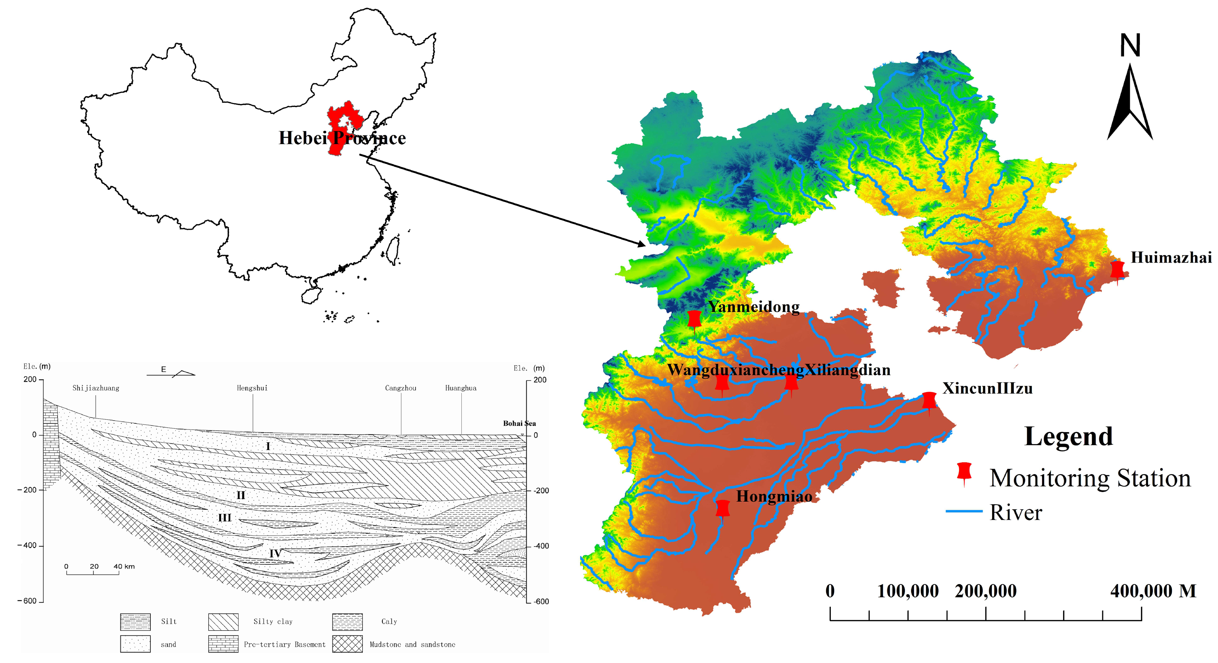
The Hebei Plain is located in North China (114°33′–119°42′ N 36°05′–39°93′ E) (Figure 1). Per capita water resources in the region are approximately 386 m3, which is approximately one eighth of China’s national average, thus making it an extremely water-scarce region. It lies in the semi-humid, semi-arid climate zone and experiences a temperate continental monsoon climate. This region has four distinct seasons with rainy and hot periods coinciding. Annual precipitation is unevenly distributed but mainly falls in summer, with an annual average of 450–550 mm. Precipitation from June to July accounts for approximately 75% of the annual precipitation, and surface water resources are relatively scarce. The main water source for irrigation is groundwater, and agricultural groundwater consumption accounts for 74.5–76.6% of groundwater exploitation.
The North China Plain has complex hydrogeological conditions, but it mainly comprises basins of Quaternary (Cenozoic) loose sediment. Quaternary aquifer media are divided into four groups (from top to bottom): Quaternary Holocene Q4, Upper Pleistocene Q3, Middle Pleistocene Q2, and Lower Pleistocene Q1. The buried depths of the bottom boundaries of the aquifer group are 40–60 m, 120–170 m, 250–350 m, and 350–550 m, respectively. Overexploitation of groundwater for many years has resulted in many groundwater cones of depression in the first, second, and third aquifer groups in the Hebei Plain, causing nonlinear changes in the groundwater flow direction and GWL height in the region.
2.2. Data Sources
GWL data collected during 2018–2020, with a time interval of 4 h, were obtained from China’s National Groundwater Monitoring Project. The trends in GWL in the Hebei Plain during the study period consisted of dynamic fluctuations, increases, and decreases. In total, six monitoring stations covering these three change types were selected as the study objects, which provided 32,880 datapoints. The time series of each station was divided, and any missing series was added so that the data could be converted into a format recognized by each model. The station data sample formats are shown in Table 1.
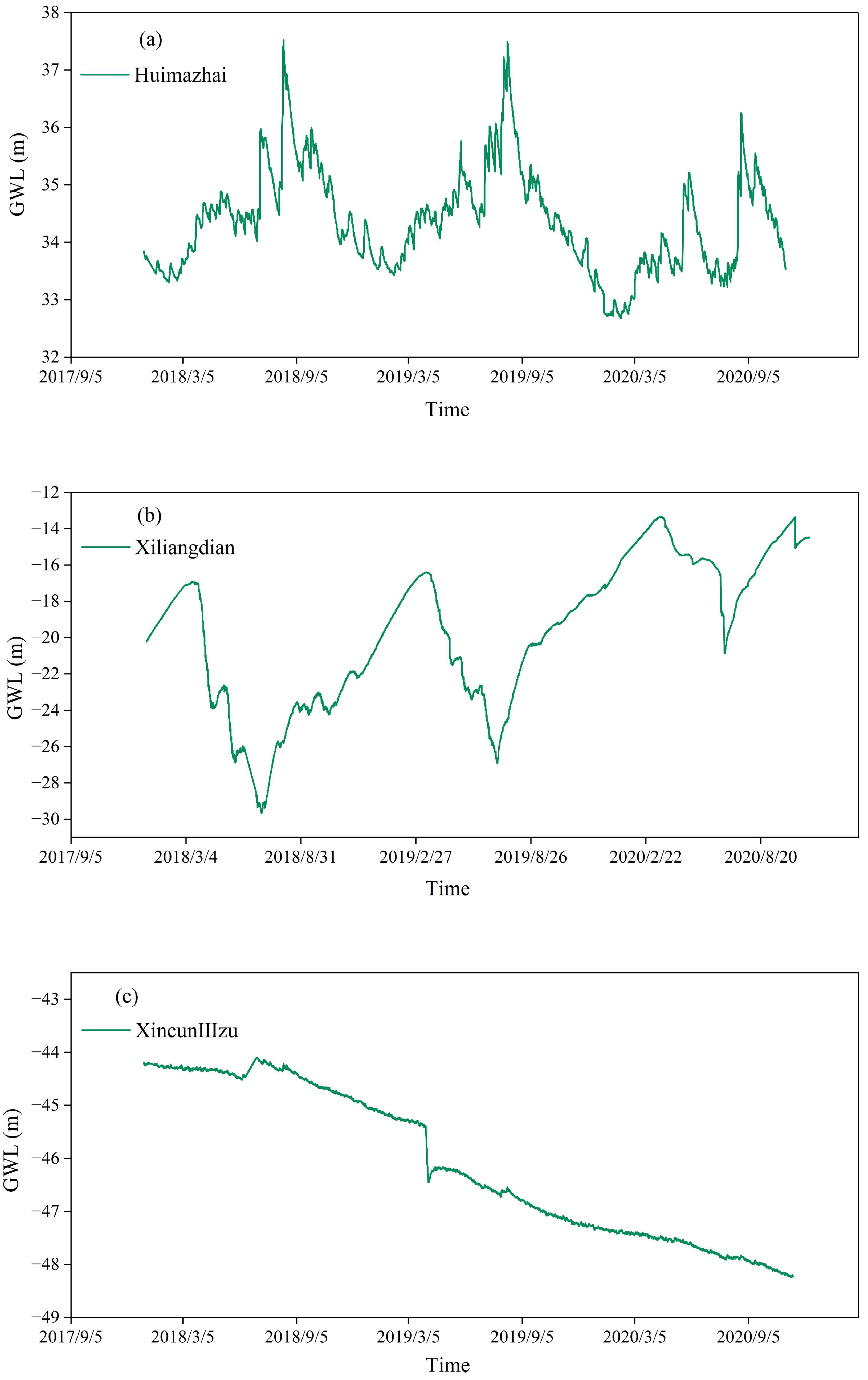
To intuitively reflect the daily changes in the GWL of the three types of selected monitoring stations, line graphs were drawn showing the time scale of GWL for 2018–2020. Figure 2a shows a station with dynamic fluctuations, where the GWL was the same at the beginning and end of the research period. Figure 2b shows a station with a dynamic increase. Although there were fluctuations during the study period, the GWL at the end of the study period was higher than at the beginning. Further, Figure 2c shows a station with a dynamic decrease, wherein the GWL at the end of the study period was lower than at the beginning.
2.3. Methods
Data-driven models, such as ANNs, can easily approximate the complex behavior and responses of physical systems; additionally, they can quickly optimize many case scenarios with different constraints. Compared with the multiple assumptions, complex input variables, and parameter calibration of physical models, the input variables of data-driven models are easier to measure and quantify. In particular, machine learning can help to predict the GWL in areas that lack hydrogeological survey data. In this study, SVM, LSTM, GRU, and MLP models were used to predict GWL at the selected monitoring stations. Each of these models has been described below.
2.3.1. Support Vector Machine
SVM is a linear discriminant classification method based on the maximum margin. SVMs are the most widely used machine learning models for predicting GWL, as they can maximize prediction accuracy. They use the linear kernel function, polynomial kernel function, Gaussian kernel radial basis function (RBF), and sigmoid kernel function, which greatly optimize the nonlinear prediction capability of the model. Moreover, it is considered the best theory for small-sample statistical estimations and predictive learning, and can precisely predict GWL.
RBF has a strong nonlinear mapping capability and is suitable for predicting moment-to-moment changes in GWL as follows:
where γ is an artificially determined positive real number parameter and (xi, xj) is the training sample.
2.3.2. Long-Short Term Memory
The LSTM model processes and analyzes time-series data by selectively extracting saved information and combining the selected information with subsequently input time-series data. The network can locally predict each fragmented sequence of GWL data, and the prediction deviations are passed back, to dynamically predict a GWL sequence.
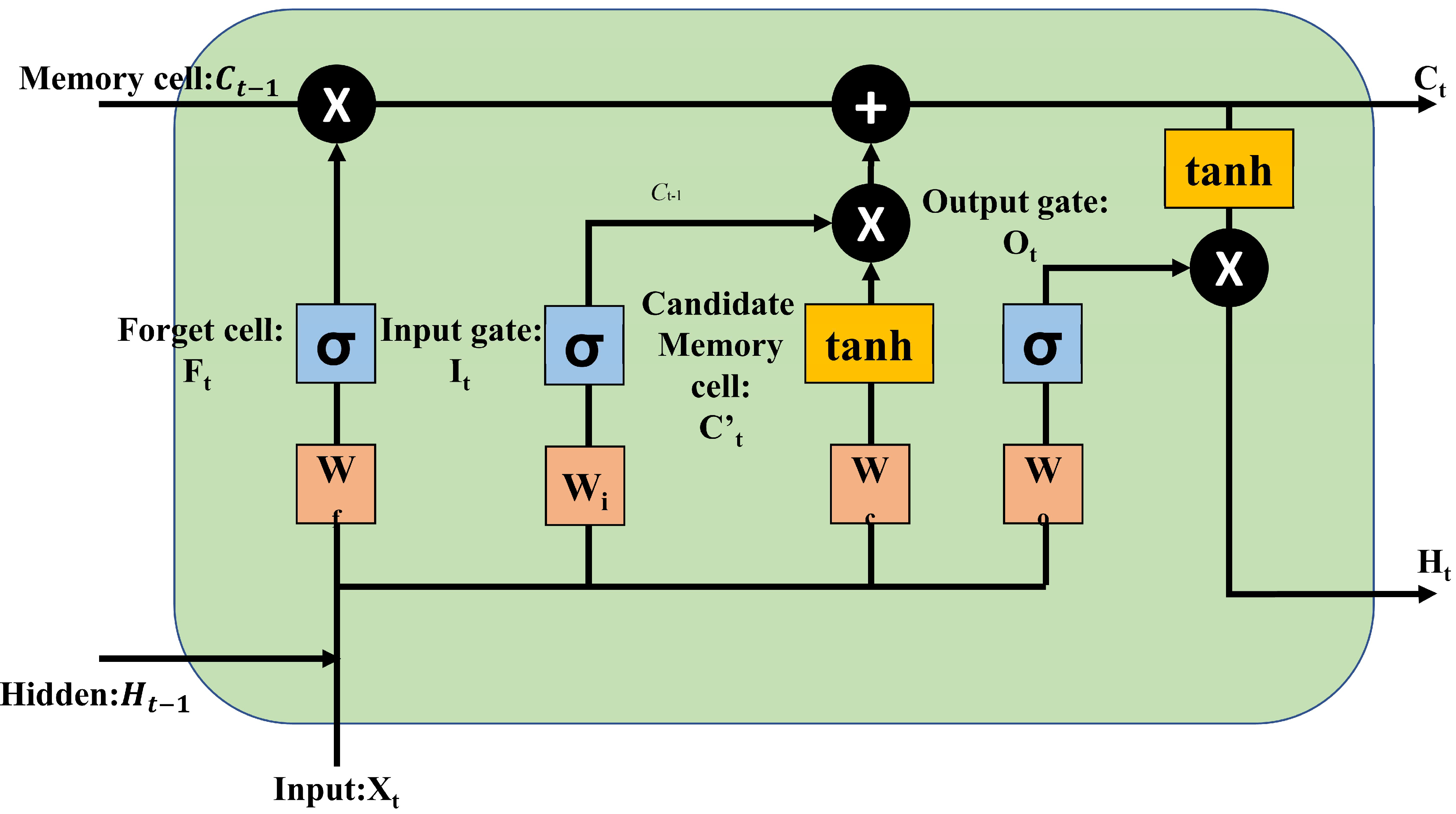
LSTM is an improved recurrent neural network (RNN). The cycle of an ordinary RNN passes through the hidden state (H), but the LSTM output has two states: H and memory state (C). Further, three “gates” are added to the LSTM to process the input information differently. Figure 3 shows the internal structure of an LSTM cell.
At the core of LSTM is the objective of controlling the internal state to allow it to retain and filter information from previous moments. LSTM has three gates (forget gate Ft, input gate It, and output gate Ot) in the hidden layer to control the signal input and output. The forget gate uses Ht−1 and Xt as inputs to control how much information needs to be forgotten in the internal state of the previous moment Ct−1; further, the input gate selectively memorizes input information and determines the quantity saved to the cell state Ct in the current moment Xt. The output gate controls how much information the internal state Ct needs to output to the external state in the current moment. The entire network equation of the LSTM cell can be given as follows:
where σ is the sigmoid activation function, which limits the output to between 0 and 1. Since each element of the output matrix (or vector) after the sigmoid layer is a real number between 0 and 1, which is then dot-multiplied with other information, it effectively controls the passage of information. In this range, “0” indicates that the information does not pass at all, and “1” indicates that the information passes entirely. This allows the network to regulate the flow of information through the “gate”.
2.3.3. Gated Recurrent Units
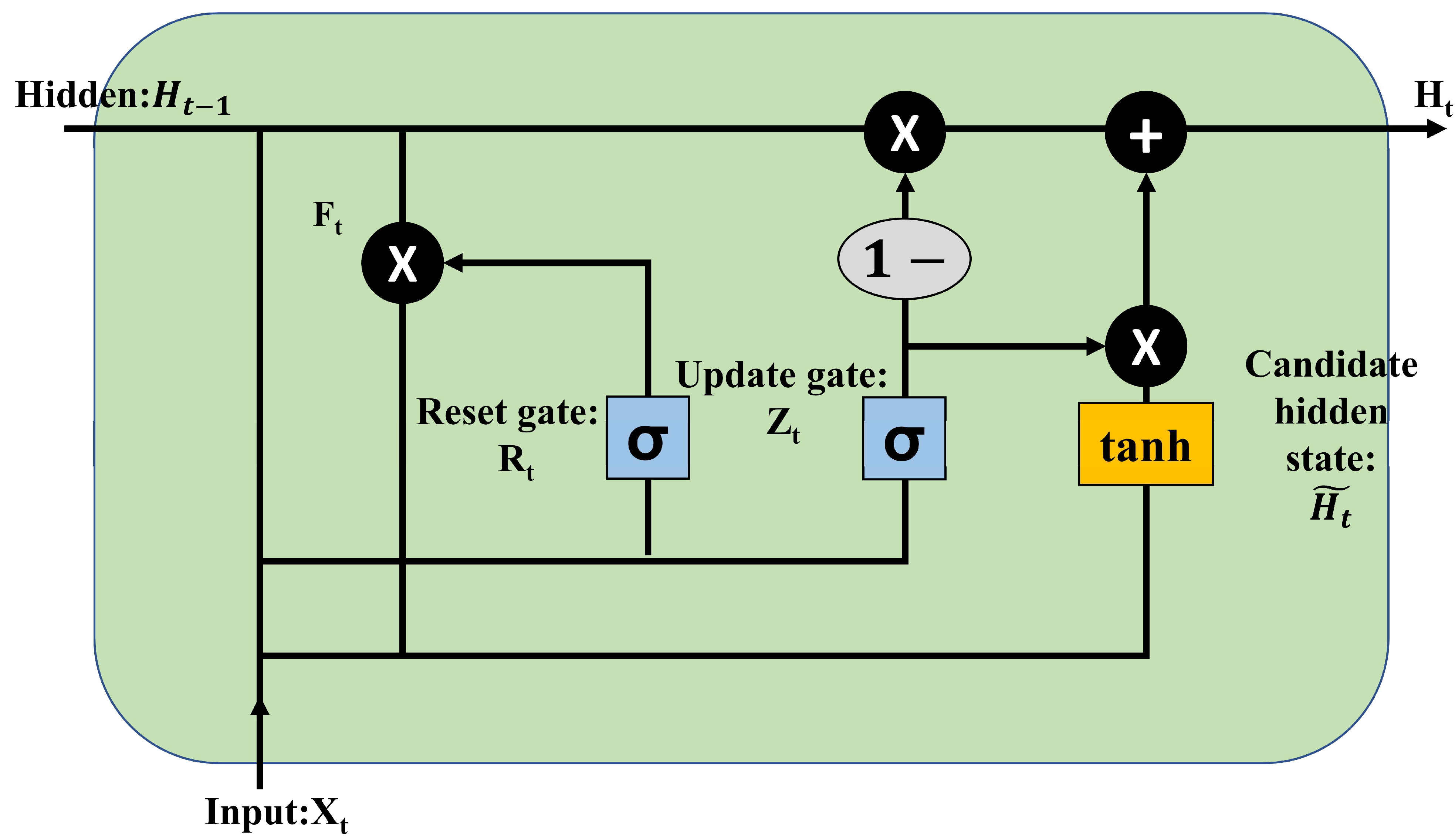
GRU optimizes the gated structure of LSTM (Figure 4), and its training process is easier to converge. Compared with LSTM, GRU has only two gates: the update and reset gates. The update gate is constructed from the forget and input gates in the LSTM. The reset gate is recomposed from memory cells and hidden layer states. The GRU network controls the change in state of hidden units over time through its special gated structure. This avoids inaccurate parameter training due to the vanishing gradient problem or exploding gradient problem during long-term propagation.
In Figure 4, the update and reset gates are denoted by Zt and Rt, respectively, where Zt is used to control the extent to which Ht−1 is retained in Ht, and Rt is used to control the extent to which the current candidate set will be written into Ht−1.
First, the gating state is obtained from the state in the previous moment Ht−1 and the input Xt in the current moment. Subsequently, using sigmoid nonlinear transformation, the data are mapped to [0,1], which acts as the gating signal. Once the gating signal has been obtained, the reset gate is “reset” as a coefficient before the previous moment Ht−1 to obtain the candidate hidden state . The equations are as follows:
where σ is the sigmoid activation function. While calculating a gate’s hidden state, the sigmoid function is used to obtain a result between 0 and 1, and while calculating a candidate hidden state, the activation function uses the tanh function. Wr, Wz, and are the reset gate, update gate, and the weight matrix, respectively, for calculating the candidate hidden state.
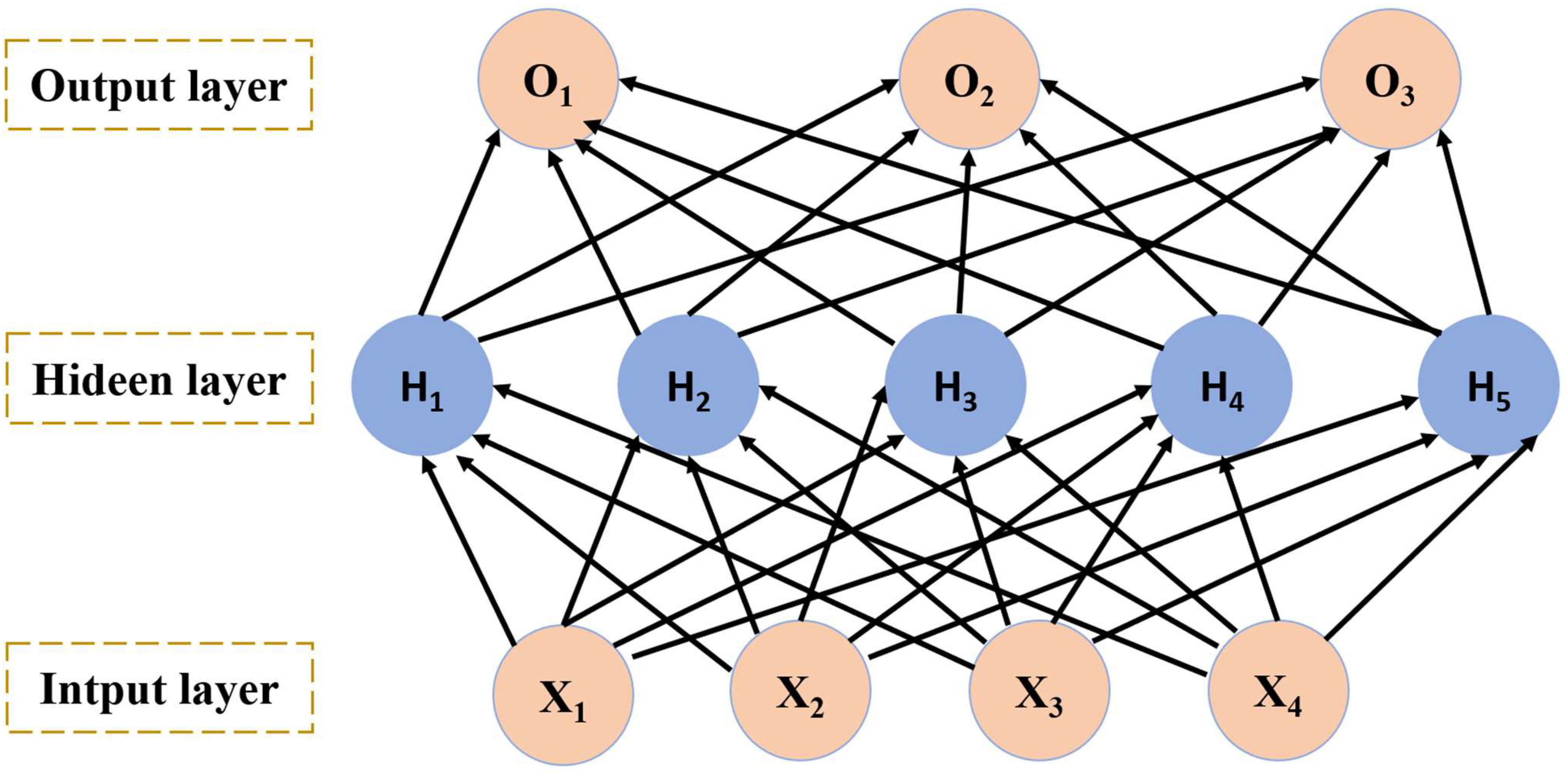
2.3.4. Multi-Layer Perceptron
MLP is an ANN used for predictions. It learns the relationships between inputs and outputs using a large volume of data and can be used for nonlinear modeling. An MLP is composed of multiple layers of neurons, and each node (neuron) in a layer is connected with a certain weight to every node in the following layer (Figure 5). The main disadvantage of this method is that when layers or the nodes in each layer increase, overfitting and model training issues arise.
In Figure 5, the output of the MLP hidden layer H node is given as
where ω and b are the weight and deviation, respectively, and g is the activation function, commonly the sigmoid, tanh, or rectifier linear unit (ReLU) activation function. Because the ReLU function avoids the vanishing gradient problem and its convergence speed is faster than that of the sigmoid and tanh activation functions, ReLU was used as the activation function in this study.
2.4. Performance Evaluation of Models
The performance of the SVM, LSTM, GRU, and MLP models can be evaluated using the root mean square error (RMSE), coefficient of determination (R2), and Nash–Sutcliffe efficiency (NSE), which are calculated as follows:
where Qo is the observed GWL, Qp is the predicted GWL, N is the length of the groundwater series, and is the mean value of the observed GWL.
2.5. Groundwater Level Prediction Methodology
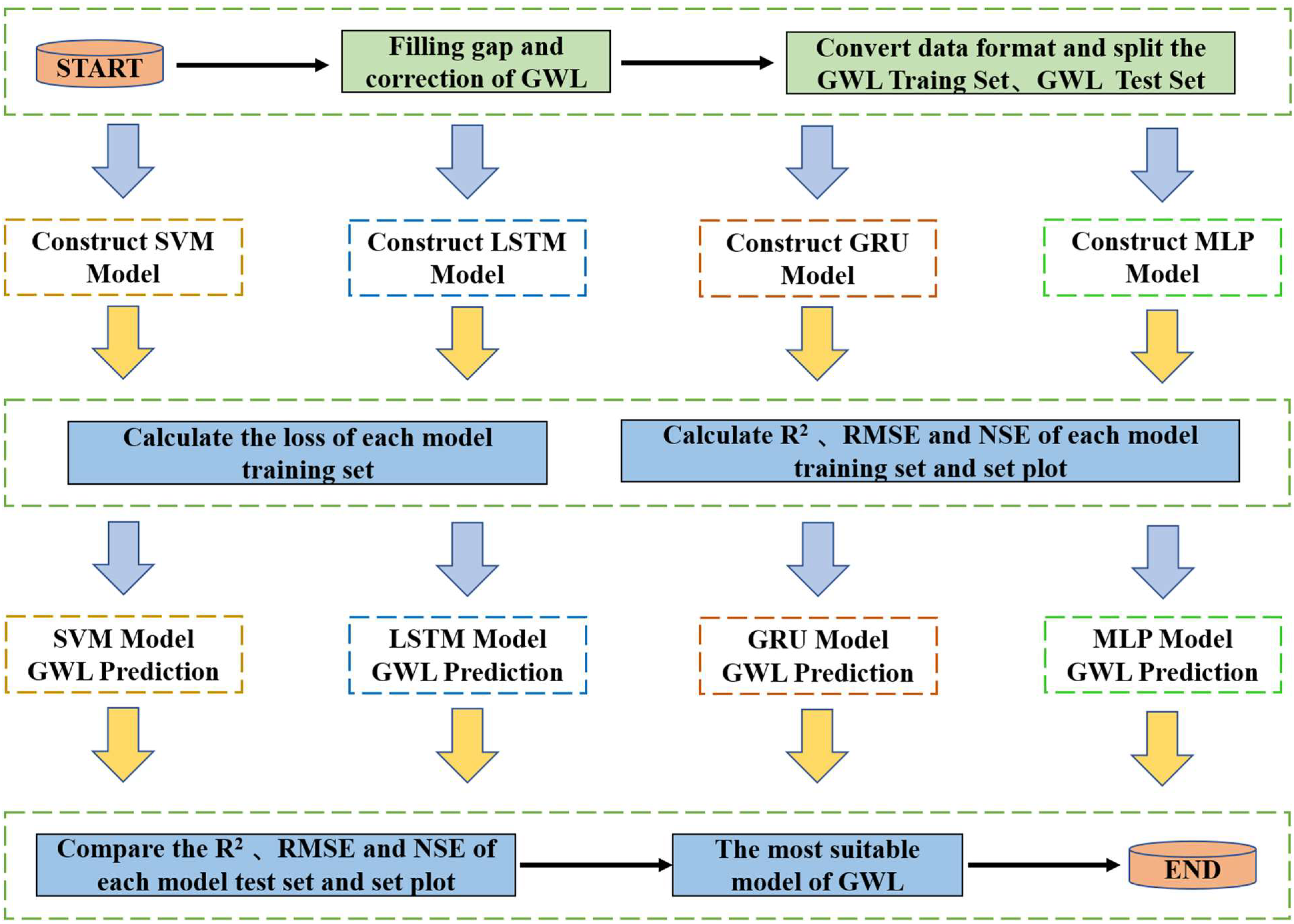
As shown in Figure 6, we first input missing values and processed outliers in the original dataset and converted the format into a data type recognized by the model. Subsequently, we split the dataset, with the first 70% of the time-scale GWL measured sequence used as the training set. We converted the one-dimensional training data into a two-dimensional matrix containing input data and testing data, with a window of 10, i.e., GWL0–GWL9 was used to predict GWL10, GWL1–GWL10 was used to predict GWL11, etc. GWL data of each station were converted into this format. Later, we used the SVM, LSTM, GRU, and MLP models to build and train the dataset, calculated the loss functions of each model, observed the consistency between predicted and actual values, and judged the robustness of each model based on its dynamic changes. The degree of convergence of the loss function was used as the basis for the training results of each model to continuously train the model. After training was completed, 30% of the time-scale GWL measured sequence for each station was used as the testing set. The testing set data were also converted into a two-dimensional matrix as described above and input into the trained model. The R2, RMSE, and NSE evaluation indicators were used to evaluate the performance of the models, to select the model that was most suitable for dynamically predicting the GWL in the Hebei Plain.
3. Results and Discussion
The results of the GWL predictions for each station in Hebei Province acquired through the machine learning techniques are presented in this section. The Huimazhai and Hongmiao stations were the dynamically fluctuating stations. The Huimazhai station is located in the urban area of Qinhuangdao, adjacent to the Shi River and Liaodong Bay, and it showed an average GWL of 34.36 m. During the study period, its GWL in summer was mostly higher than in spring and winter, resulting in dynamic fluctuations. This may be due to a reduced need to irrigate crops in the rainy and summer season across the entire Qinhuangdao area. Moreover, changes in GWL were consistent with changes in precipitation. The Hongmiao station is located in Xingtai City, where groundwater is exploited for crop irrigation. However, Xingtai has conducted a groundwater restoration pilot project and promoted the cultivation of drought-resistant winter wheat; additionally, groundwater replenishment work has also been conducted. The GWL in this area fluctuated due to the influence of changes in human activities, but it had a mean GWL of −65.09 m. The dynamically increasing stations were Xiliangdian and Yanmeidong. The Xiliangdian station is located in Gaoyang County, Baoding, and had a mean GWL of −19.41 m. The GWL in this station was lower in spring and summer than in other seasons, which was likely due to the expansive area of water-intensive crops in spring and summer. Nevertheless, because this area is located in the middle route of the South-to-North Water Diversion Project, its GWL has been increasing. Further, the Yanmeidong station is located in Laiyuan County, Baoding, and showed an average GWL of 1235.67 m, and its GWL increased overall during the study period. This was likely due to the station being located in a mountainous area that receives relatively high levels of precipitation; moreover, because the area under irrigated farmland in the region was small, agricultural water consumption was low. The dynamically decreasing stations were Wangduxiancheng and XincunIIIzu. The Wangduxiancheng station is located in Wangdu County, Baoding, and had a mean GWL of 16.43 m, and XincunIIIzu is located in Huanghua and had a mean GWL of −43.13 m. Despite the implementation of groundwater extraction projects at the two stations, their water levels decreased gradually during the study period due to increases in the area under winter wheat.
In this study, GWL data were divided into training and validation sets, with the GWL of the validation set predicted using mathematical relationships discovered in the training set data. The SVM, LSTM, GRU, and MLP models were used to develop a GWL prediction model, and time-series scatter plots, relative error, and Taylor diagrams were used to qualitatively evaluate the performance of the models, while statistical and hydrological model indicators, such as RMSE, R2, and NSE, were used to quantitatively evaluate their performance.
3.1. GWL Prediction Using SVM Model
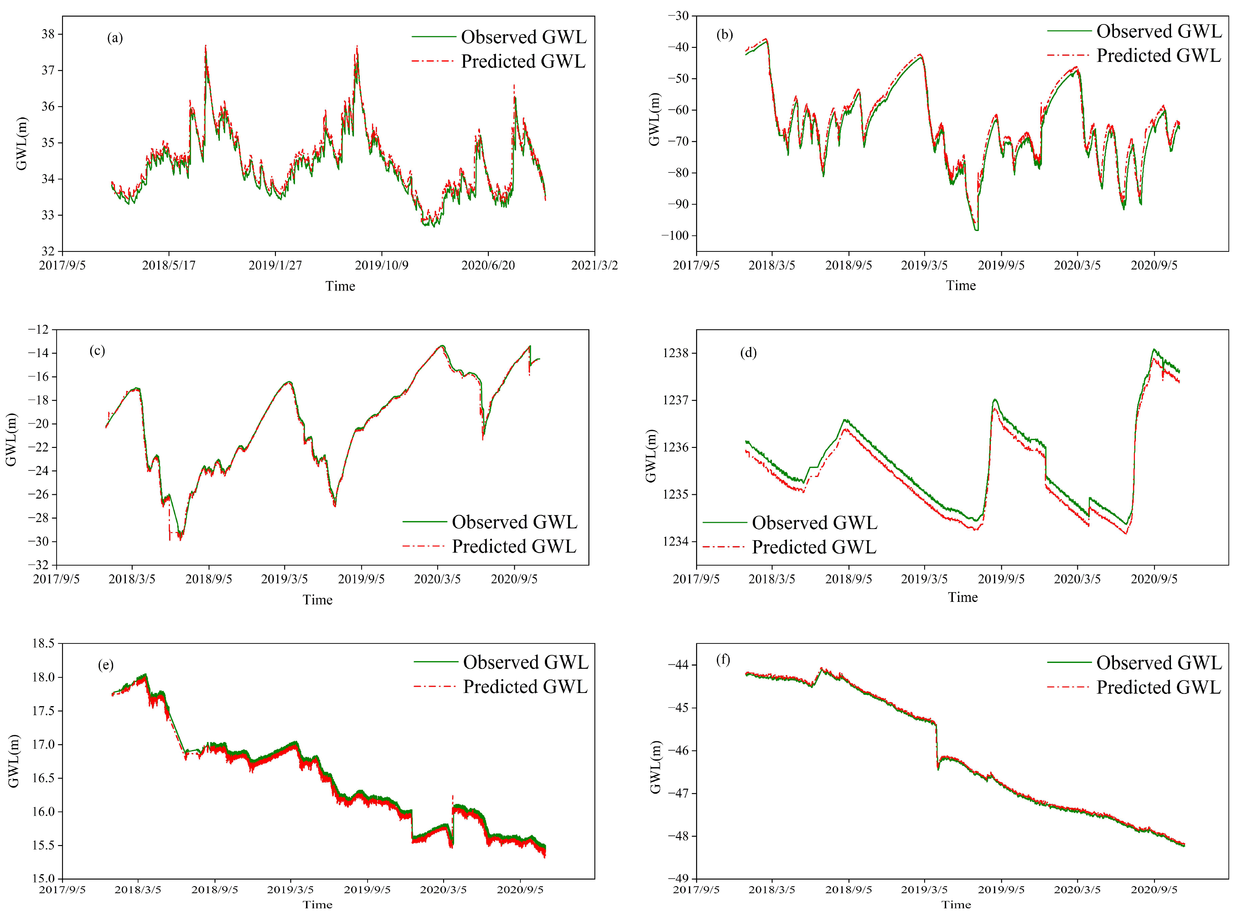
Gaussian and linear kernel functions were used for SVM-based runoff modeling. The former was more effective than the latter; therefore, we established an SVM model with the Gaussian function as the kernel function to predict the GWL of the six monitoring stations with the three types of dynamic changes (fluctuations, increases, and decreases). As shown in Figure 7, the SVM model overestimated the GWL of the dynamically fluctuating stations and slightly underestimated the GWL of the stations with dynamic increases and decreases.
Table 2 shows the simulation results. Generally, the simulation results were better for the dynamically increasing and decreasing stations. For example, the RMSE, R2, and NSE values of the Yanmeidong station in the testing period were 0.193 m, 0.998, and 0.984, respectively, indicating that SVM was well suited to these two types of monitoring stations. Considering the dynamically fluctuating stations, the RMSE, R2, and NSE values of the Huimazhai station in the training period were 0.253 m, 0.953, and 0.921, respectively, while the accuracy in the testing period was markedly lower, with NSE being 24.9% lower in the testing period than in the training period, indicating that SVM was not effective at capturing the nonlinear relationship of dynamically fluctuating stations. Overall, SVM was not suitable for predicting GWL in the Hebei Plain.
3.2. GWL Prediction Using the LSTM Model
During LSTM modeling, the model filtered GWL features through the output gate, saved the useful features, and discarded the useless features to obtain current moment contextual information, which greatly enriched the information in the vector. This also implied that the current moment contextual information Ht was only one part of the global information Ct. Further, we used the LSTM model to simulate the six selected stations. The GWL in the training and testing periods is shown in Figure 8. The GWL prediction results were suboptimal for the dynamically fluctuating stations, including another overestimation of the peak value in the testing period shown in Figure 8a. However, compared with the SVM model, the results of the dynamically increasing station, shown in Figure 8d, improved, with the predicted GWL closer to the observed GWL, although the peak value was overestimated.
Table 3 shows the simulation results. The RMSE, R2, and NSE values of the Yanmeidong station in the testing period were 0.116 m, 0.996, and 0.994, respectively. Notably, the results from the testing period were better than those from the training period for this station, indicating that the observed and predicted values in the verification period were highly consistent, thus proving the effectiveness of the LSTM model for the dynamically increasing stations. The RMSE, R2, and NSE values of the Huimazhai station in the training period were 0.263 m, 0.868, and 0.868, respectively. Compared to the R2 value of the SVM model, the R2 value of the LSTM model was 12.7% higher. Nevertheless, for the dynamically fluctuating stations, both the peaks and troughs of the predicted GWL were more than the observed GWL; therefore, the prediction results were suboptimal. The overall R2 value of the LSTM model was >0.85, indicating that it was a good model for predicting the GWL in the Hebei Plain.
3.3. GWL Prediction Using the MLP Model
The MLP model includes the input, output, and hidden layers, and each node (neuron) in a layer is connected to every node in the following layer. We improved the basic three-layer MLP by adding two linear hidden layers and the ReLU activation function after the first hidden layer. Subsequently, we simulated the selected stations in the Hebei Plain. Notably, this model solved the shortcomings of the SVM and LSTM models for dynamically fluctuating stations (Figure 9a,b). The predicted trend was satisfactory and higher in the testing period than in the training period. However, in the stations with dynamically increasing trends (Figure 8c), further improvement in the prediction results of peak and trough values was not possible.
Table 4 shows the simulation results. The RMSE, R2, and NSE values of the Yanmeidong station in the testing period were 0.08 m, 0.998, and 0.997, respectively, which were the best simulation results. The results for the dynamically fluctuating stations (Huimazhai and Hongmiao) were also satisfactory, especially for the Huimazhai station, with RMSE, R2, and NSE values of 0.201 m, 0.959, and 0.95 in the training period and 0.128 m, 0.979, and 0.968 in the testing period, respectively. Thus, the results in the testing period were better than those in the training period. Overall, the RMSE values of the various station types were <0.6, and NSE and R2 values were >0.96, thus making this a highly suitable model for predicting the GWL in the Hebei Plain.
3.4. GWL Prediction Using the GRU Model
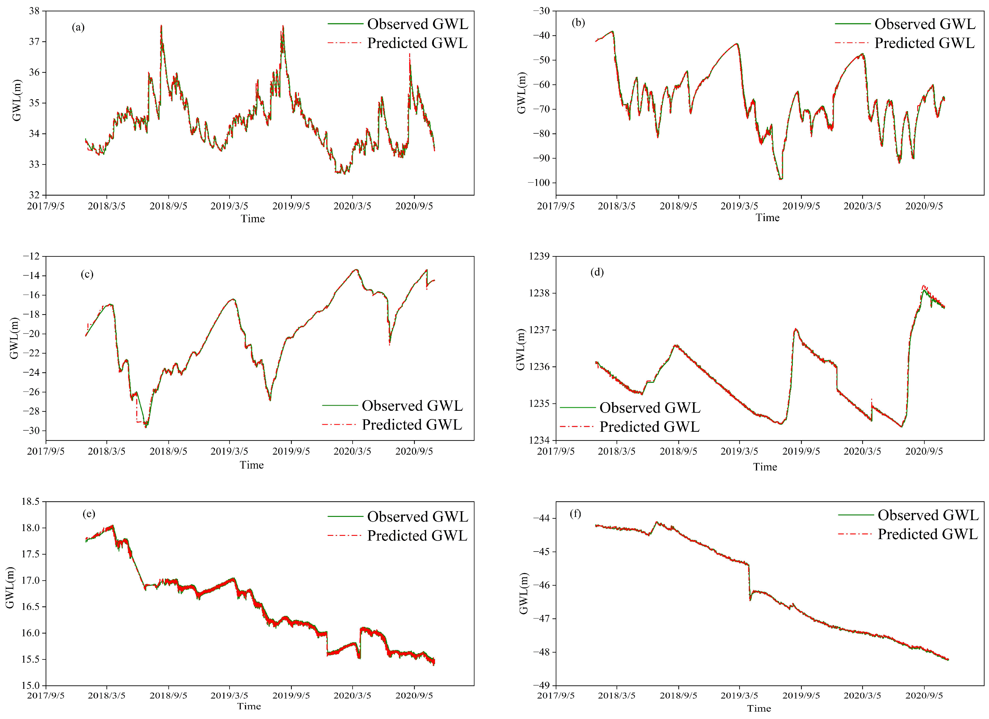
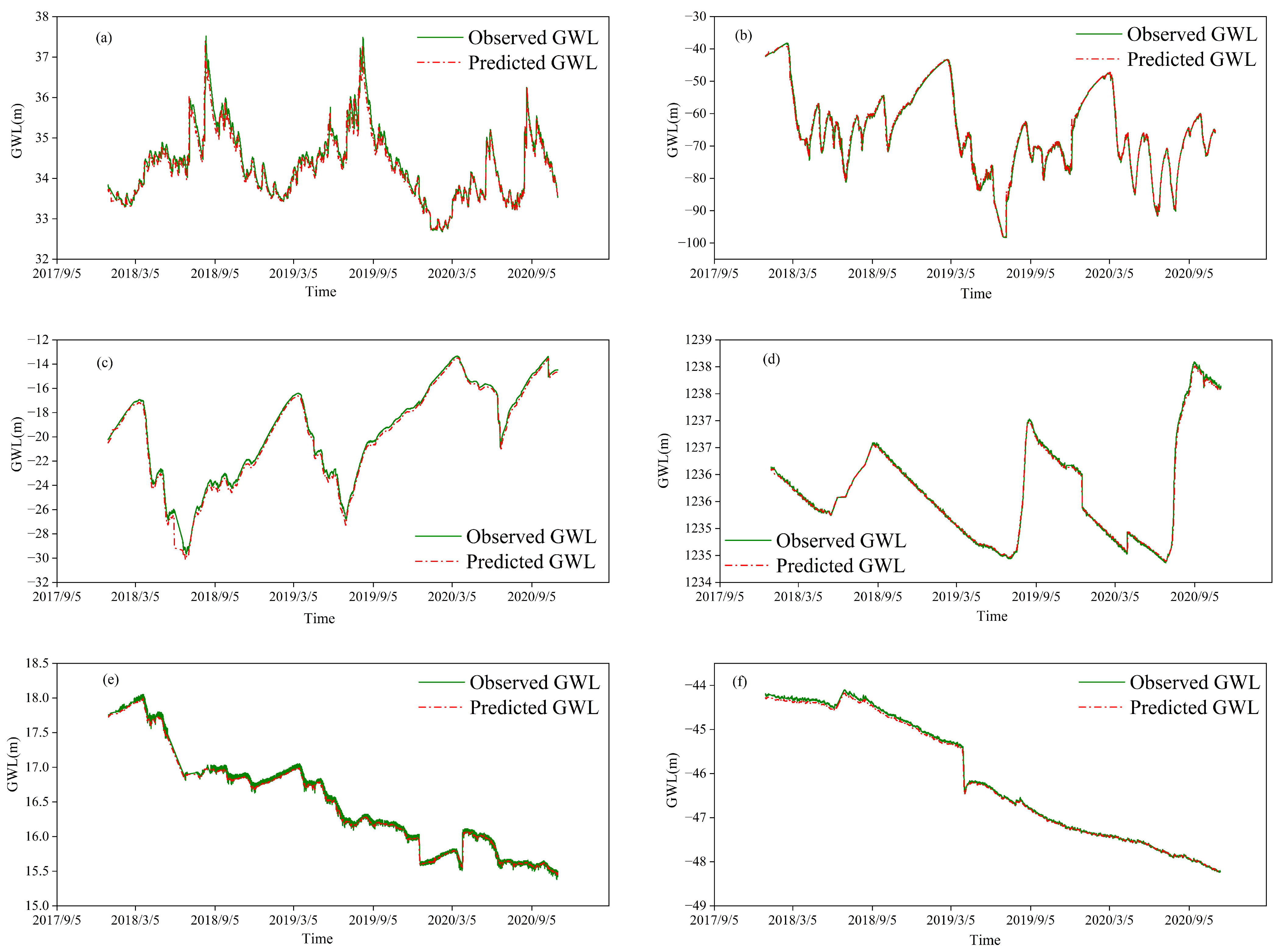
Compared with LSTM, GRU has a simpler gated structure and fewer parameters and faster convergence. The Ct in GRU already contained Ht, and there was a trade-off between current unit information and previous global information while generating moment contextual information. Therefore, replacing It with 1-Zt can expose all information globally. The GRU model for each of the selected stations in the training and testing periods is shown in Figure 10. The model retained the testing results of the MLP model for dynamically fluctuating stations, but the testing period results for the dynamically increasing station (c) were better than the results of the other models.
Table 5 shows the corresponding simulation results. The best training period results were observed in the XincunIIIzu station, with RMSE, R2, and NSE values of 0.081 m, 0.999, and 0.996, respectively, while the best testing period results were observed in the Yanmeidong station, with RMSE, R2, and NSE values of 0.098 m, 0.998, and 0.996, respectively. The GRU model results were notably better for dynamically fluctuating stations than those of the first three models. Furthermore, the model maintained the training and testing results for the other station types, thus making it the best model for predicting the GWL in the Hebei Plain.
3.5. Model Comparison
The SVM model had the lowest simulation accuracy for the selected stations, which may be due to the four kernel functions of the SVM. The RBF kernel function selected in this study could be modified further. When σ is too small, RBF can overfit, and when σ is too large, the relationship between Xi and Xj will have less overall influence on the model, causing inaccurate predictions. The LSTM model was the third-best model. It included a forget gate, which makes the partial derivative of the current memory unit to the previous memory unit a constant, thereby solving the disappearing gradient problem of RNN. Nevertheless, several input parameters exist, which increase the likelihood of overfitting. The second-best model was MLP. Its highly nonlinear global effect resulted in good accuracy in the training and testing periods, with an NSE value of 0.997 for the Yanmeidong station, but the model had the slowest learning speed, which was suboptimal in terms of time consumption for moment-to-moment predictions. Moreover, the GRU model was the most accurate for the dynamically fluctuating and dynamically increasing stations. As it had a simple gated structure and fewer input parameters, and as it reduced the risk of overfitting, it had a shorter training time (Table 6). Thus, it was the most suitable model for predicting the GWL in the Hebei Plain.
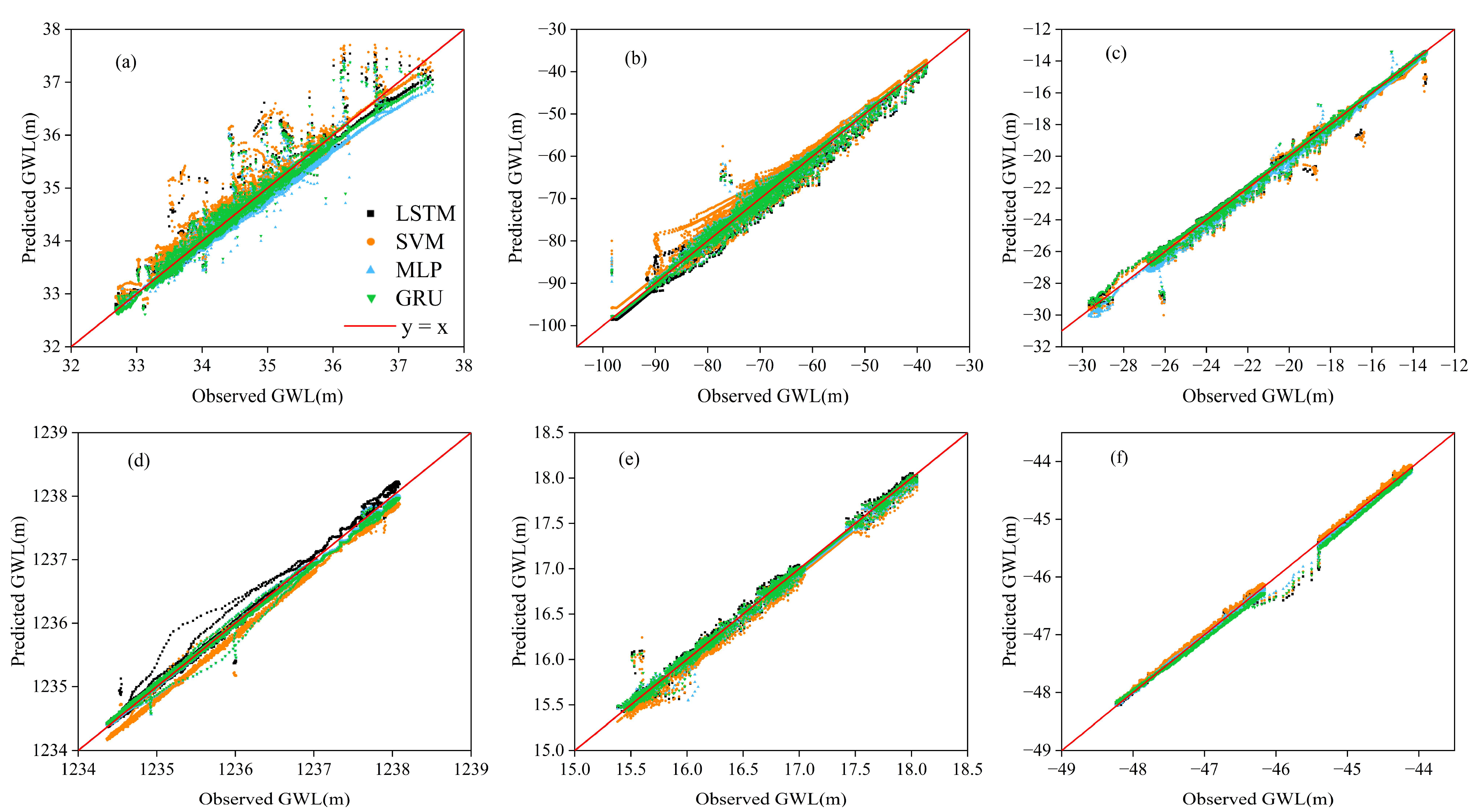
Figure 11 presents the scatter plots for each station during the study period. The GRU model had the best correlation between the observed and predicted GWL of the four models, with predicted values near the regression function for almost every station. Although the MLP model was accurate for most stations, it did not capture the extreme values of the dynamically increasing sites. Moreover, the SVM and LSTM models only reflected the GWL trend for dynamically fluctuating stations, and they did not accurately predict the specific GWL values.
Finally, we evaluated the performance of the models for each of the stations using Taylor diagrams (Figure 12). The results showed that the GRU model had the best accuracy for both dynamically fluctuating and dynamically increasing stations, followed by the MLP model, which had the best accuracy for dynamically decreasing stations. Comparatively, the SVM model had the poorest performance, as it was the furthest from the “Ref” point for most stations. It was followed by the LSTM model, which performed reasonably.
4. Conclusions
GWL is a crucial indicator for evaluating the health of groundwater resources in the Hebei Plain. This study attempted to model the GWL in the Hebei Plain and predict dynamic changes in the GWL using SVM, LSTM, MLP, and GRU models, and it qualitatively and quantitatively analyzed the training and testing datasets in the modeling process. The main conclusions were as follows:
- (1)
- By comparing the RMSE, R2, and NSE indicators, we discovered that the GRU model performed the best for dynamically fluctuating and dynamically increasing stations, while the MLP model performed the best for dynamically decreasing stations. The update gate in the GRU model acquired previous moment state information in the current state, which assisted in capturing long-term dependencies in the time series and solved the problem of overfitting to some extent. Moreover, the GRU model not only showed good performance in predicting trends, but it was also better than the other models regarding the training time and capturing extreme values, thus making it the most suitable model for predicting the GWL in the Hebei Plain.
- (2)
- Apart from the different principles of each model, the differences in the simulation results can be attributed to factors such as data segmentation during the modeling process, the length of subsequences, and the uncertainty of model parameters. Moreover, the influence of the different activation functions on the GWL in the different models should also be considered. Furthermore, the training frequency of each model in this study was the same, and adaptive improvements should be made for each model in subsequent studies.
Author Contributions
Conceptualization, Z.W. and C.W.; methodology, Z.W.; software, C.L.; validation, Q.S., W.L. and X.H.; investigation, Z.W., C.W. and T.Q.; resources, Q.S.; data curation, C.W.; writing—original draft preparation, Q.S. and Z.W.; writing—review and editing, C.W.; visualization, Q.S.; supervision, W.L.; project administration, L.Y.; funding acquisition, C.L. All authors have read and agreed to the published version of the manuscript.
Funding
This research was funded by the National Key Research and Development Program of China (2021YFC3000205), Heilongjiang Provincial Applied Technology Research and Development Program (GA19C005), Key R & D Program of Heilongjiang Province (JD22B001), and Independent Research Project of the State Key Laboratory of Simulation and Regulation of Water Cycle in River Basin (SKL2022ZD02).
Data Availability Statement
The data will be available on request.
Acknowledgments
The authors would like to thank the editor and two anonymous reviewers for taking the time to provide their helpful feedback and suggestions.
Conflicts of Interest
The authors declare no conflict of interest.
References
- Wei, Y.; Sun, B. Optimizing Water Use Structures in Resource-Based Water-Deficient Regions Using Water Resources Input–Output Analysis: A Case Study in Hebei Province, China. Sustainability 2021, 13, 3939. [Google Scholar] [CrossRef]
- Currell, M.J.; Han, D.; Chen, Z.; Cartwright, I. Sustainability of groundwater usage in northern China: Dependence on palaeowaters and effects on water quality, quantity and ecosystem health. Hydrol. Process. 2012, 26, 4050–4066. [Google Scholar] [CrossRef]
- Niu, J.; Zhu, X.G.; Parry, M.A.J.; Kang, S.; Du, T.; Tong, L.; Ding, R. Environmental burdens of groundwater extraction for irrigation over an inland river basin in Northwest China. J. Clean. Prod. 2019, 222, 182–192. [Google Scholar] [CrossRef] [Green Version]
- Gupta, B.B.; Nema, A.K.; Mittal, A.K.; Maurya, N.S. Modeling of Groundwater Systems: Problems and Pitfalls. Available online: https://www.researchgate.net/profile/Atul-Mittal-3/publication/261758986_Modeling_of_Groundwater_Systems_Problems_and_Pitfalls/links/00b495356b45d3464c000000/Modeling-of-Groundwater-Systems-Problems-and-Pitfalls.pdf (accessed on 2 December 2022).
- Ahmadi, S.H.; Sedghamiz, A. Geostatistical analysis of spatial and temporal variations of groundwater level. Environ. Monit. Assess. 2007, 129, 277–294. [Google Scholar] [CrossRef] [PubMed]
- Chen, H.; Zhang, W.; Nie, N.; Guo, Y. Long-term groundwater storage variations estimated in the Songhua River Basin by using GRACE products, land surface models, and in-situ observations. Sci. Total Environ. 2019, 649, 372–387. [Google Scholar] [CrossRef] [PubMed]
- Sahoo, S.; Russo, T.A.; Elliott, J.; Foster, I. Machine learning algorithms for modeling groundwater level changes in agricultural regions of the US. Water Resour. Res. 2017, 53, 3878–3895. [Google Scholar] [CrossRef] [Green Version]
- Yadav, B.; Ch, S.; Mathur, S.; Adamowski, J. Assessing the suitability of extreme learning machines (ELM) for groundwater level prediction. J. Water Land Dev. 2017, 32, 103–112. [Google Scholar] [CrossRef]
- Xiong, J.; Guo, S.; Kinouchi, T. Leveraging machine learning methods to quantify 50 years of dwindling groundwater in India. Sci. Total Environ. 2022, 835, 155474. Available online: https://www.sciencedirect.com/science/article/abs/pii/S0048969722025700 (accessed on 3 December 2022). [CrossRef]
- Pratoomchai, W.; Kazama, S.; Hanasaki, N.; Ekkawatpanit, C.; Komori, D. A projection of groundwater resources in the Upper Chao Phraya River basin in Thailand. Hydrol. Res. Lett. 2014, 8, 20–26. [Google Scholar]
- Thomas, B.F.; Famiglietti, J.S.; Landerer, F.W.; Wiese, D.N.; Molotch, N.P.; Argus, D.F. GRACE groundwater drought index: Evaluation of California Central Valley groundwater drought. Remote Sens. Environ. 2017, 198, 384–392. [Google Scholar] [CrossRef]
- Vapnik, V.N. The Nature of Statistical Learning Theory; Springer: New York, NY, USA, 1995; p. 314. [Google Scholar]
- Scholkoff, B.; Smola, A.J. Learning with Kernels: Support Vector Machines, Regularization, Optimization, and Beyond; MIT Press: Cambridge, MA, USA, 2002; p. 648. [Google Scholar]
- Asefa, T.; Kemblowski, M.W.; Urroz, G.; McKee, M.; Khalil, A. Support vectors–based groundwater head observation networks design. Water Resour. Res. 2004, 40, 11. Available online: https://agupubs.onlinelibrary.wiley.com/doi/abs/10.1029/2004WR003304 (accessed on 3 December 2022). [CrossRef] [Green Version]
- Yoon, H.; Jun, S.C.; Hyun, Y.; Bae, G.-O.; Lee, K.-K. A comparative study of artificial neural networks and support vector machines for predicting groundwater levels in a coastal aquifer. J. Hydrol. 2011, 396, 128–138. [Google Scholar] [CrossRef]
- Tapak, L.; Rahmani, A.R.; Moghimbeigi, A. Prediction the groundwater level of Hamadan-Bahar plain, west of Iran using support vector machines. J. Res. Health Sci. 2013, 14, 82–87. [Google Scholar]
- Sudheer, C.; Maheswaran, R.; Panigrahi, B.K.; Mathur, S. A hybrid SVM-PSO model for forecasting monthly streamflow. Neural Comput. Appl. 2014, 24, 1381–1389. [Google Scholar] [CrossRef]
- Wang, W.; Xu, D.; Chau, K.; Chen, S. Improved annual rainfall-runoff forecasting using PSO–SVM model based on EEMD. J. Hydroinformatics 2013, 15, 1377–1390. [Google Scholar] [CrossRef]
- Hochreiter, S.; Schmidhuber, J. Long short-term memory. Neural Comput. 1997, 9, 1735–1780. [Google Scholar] [CrossRef]
- Vu, M.T.; Jardani, A.; Massei, N.; Fournier, M. Reconstruction of missing groundwater level data by using Long Short-Term Memory (LSTM) deep neural network. J. Hydrol. 2021, 597, 125776. [Google Scholar] [CrossRef]
- Wunsch, A.; Liesch, T.; Broda, S. Groundwater level forecasting with artificial neural networks: A comparison of long short-term memory (LSTM), convolutional neural networks (CNNs), and non-linear autoregressive networks with exogenous input (NARX). Hydrol. Earth Syst. Sci. 2021, 25, 1671–1687. [Google Scholar] [CrossRef]
- Haykin, S. Neural Networks and Learning Machines, 3/E; Pearson Education India: New Delhi, India, 2009; Available online: https://www.pearson.com/en-us/subject-catalog/p/neural-networks-and-learning-machines/P200000003278 (accessed on 4 December 2022).
- Foddis, M.L.; Montisci, A.; Trabelsi, F.; Uras, G. An MLP-ANN-based approach for assessing nitrate contamination. Water Supply 2019, 19, 1911–1917. [Google Scholar] [CrossRef]
- Ghorbani, M.A.; Deo, R.C.; Karimi, V.; Yaseen, Z.M.; Terzi, O. Implementation of a hybrid MLP-FFA model for water level prediction of Lake Egirdir, Turkey. Stoch. Environ. Res. Risk Assess. 2018, 32, 1683–1697. [Google Scholar] [CrossRef]
- Singh, A.; Imtiyaz, M.; Isaac, R.K.; Denis, D.M. Comparison of soil and water assessment tool (SWAT) and multilayer perceptron (MLP) artificial neural network for predicting sediment yield in the Nagwa agricultural watershed in Jharkhand, India. Agric. Water Manag. 2012, 104, 113–120. [Google Scholar] [CrossRef]
- Jia, X.; Cao, Y.; O’Connor, D.; Zhu, J.; Tsang, D.C.; Zou, B.; Hou, D. Mapping soil pollution by using drone image recognition and machine learning at an arsenic-contaminated agricultural field. Environ. Pollut. 2021, 270, 116281. [Google Scholar] [CrossRef] [PubMed]
- Ijlil, S.; Essahlaoui, A.; Mohajane, M.; Essahlaoui, N.; Mili, E.M.; Van Rompaey, A. Machine Learning Algorithms for Modeling and Mapping of Groundwater Pollution Risk: A Study to Reach Water Security and Sustainable Development (Sdg) Goals in a Mediterranean Aquifer System. Remote Sens. 2022, 14, 2379. [Google Scholar] [CrossRef]
- Cho, K.; Van Merriënboer, B.; Gulcehre, C.; Bahdanau, D.; Bougares, F.; Schwenk, H.; Bengio, Y. Learning phrase representations using RNN encoder-decoder for statistical machine translation. arXiv 2014, arXiv:1406.1078. Available online: https://arxiv.org/abs/1406.1078 (accessed on 4 December 2022).
- Jeong, J.; Park, E. Comparative applications of data-driven models representing water table fluctuations. J. Hydrol. 2019, 572, 261–273. [Google Scholar] [CrossRef]
- Zhang, D.; Lindholm, G.; Ratnaweera, H. Use long short-term memory to enhance Internet of Things for combined sewer overflow monitoring. J. Hydrol. 2018, 556, 409–418. [Google Scholar] [CrossRef]
- Chen, Y.; Liu, G.; Huang, X.; Chen, K.; Hou, J.; Zhou, J. Development of a surrogate method of groundwater modeling using gated recurrent unit to improve the efficiency of parameter auto-calibration and global sensitivity analysis. J. Hydrol. 2021, 598, 125726. [Google Scholar] [CrossRef]
Figure 1.
Location and hydrogeological profile of the study area in the Hebei Plain.

Figure 2.
Three types of GWL data samples: (a) dynamic fluctuations; (b) dynamic increase; (c) dynamic decrease.
Figure 2.
Three types of GWL data samples: (a) dynamic fluctuations; (b) dynamic increase; (c) dynamic decrease.

Figure 3.
Structure of the LSTM cell.

Figure 4.
Structure of the GRU cell.

Figure 5.
Structure of MLP model.

Figure 6.
Running process of the SVM, LSTM, GRU, and MLP models.

Figure 7.
Results of hourly GWL simulation (m) in six stations using the SVM model during 2018–2020 in the training and testing periods: (a) Huimazhai station, (b) Hongmiao station, (c) Xiliangdian station, (d) Yanmeidong station, (e) Wangduxiancheng station, and (f) XincunIIIzu station.
Figure 7.
Results of hourly GWL simulation (m) in six stations using the SVM model during 2018–2020 in the training and testing periods: (a) Huimazhai station, (b) Hongmiao station, (c) Xiliangdian station, (d) Yanmeidong station, (e) Wangduxiancheng station, and (f) XincunIIIzu station.

Figure 8.
Results of the hourly GWL simulation (m) in six stations using the LSTM model during 2018–2020 in the training and testing periods: (a) Huimazhai station, (b) Hongmiao station, (c) Xiliangdian station, (d) Yanmeidong station, (e) Wangduxiancheng station, and (f) XincunIIIzu station.
Figure 8.
Results of the hourly GWL simulation (m) in six stations using the LSTM model during 2018–2020 in the training and testing periods: (a) Huimazhai station, (b) Hongmiao station, (c) Xiliangdian station, (d) Yanmeidong station, (e) Wangduxiancheng station, and (f) XincunIIIzu station.

Figure 9.
Results of hourly GWL simulation (m) in six stations using the MLP model during 2018–2020 during the training and testing periods: (a) Huimazhai station, (b) Hongmiao station, (c) Xiliangdian station, (d) Yanmeidong station, (e) Wangduxiancheng station, and (f) XincunIIIzu station.
Figure 9.
Results of hourly GWL simulation (m) in six stations using the MLP model during 2018–2020 during the training and testing periods: (a) Huimazhai station, (b) Hongmiao station, (c) Xiliangdian station, (d) Yanmeidong station, (e) Wangduxiancheng station, and (f) XincunIIIzu station.

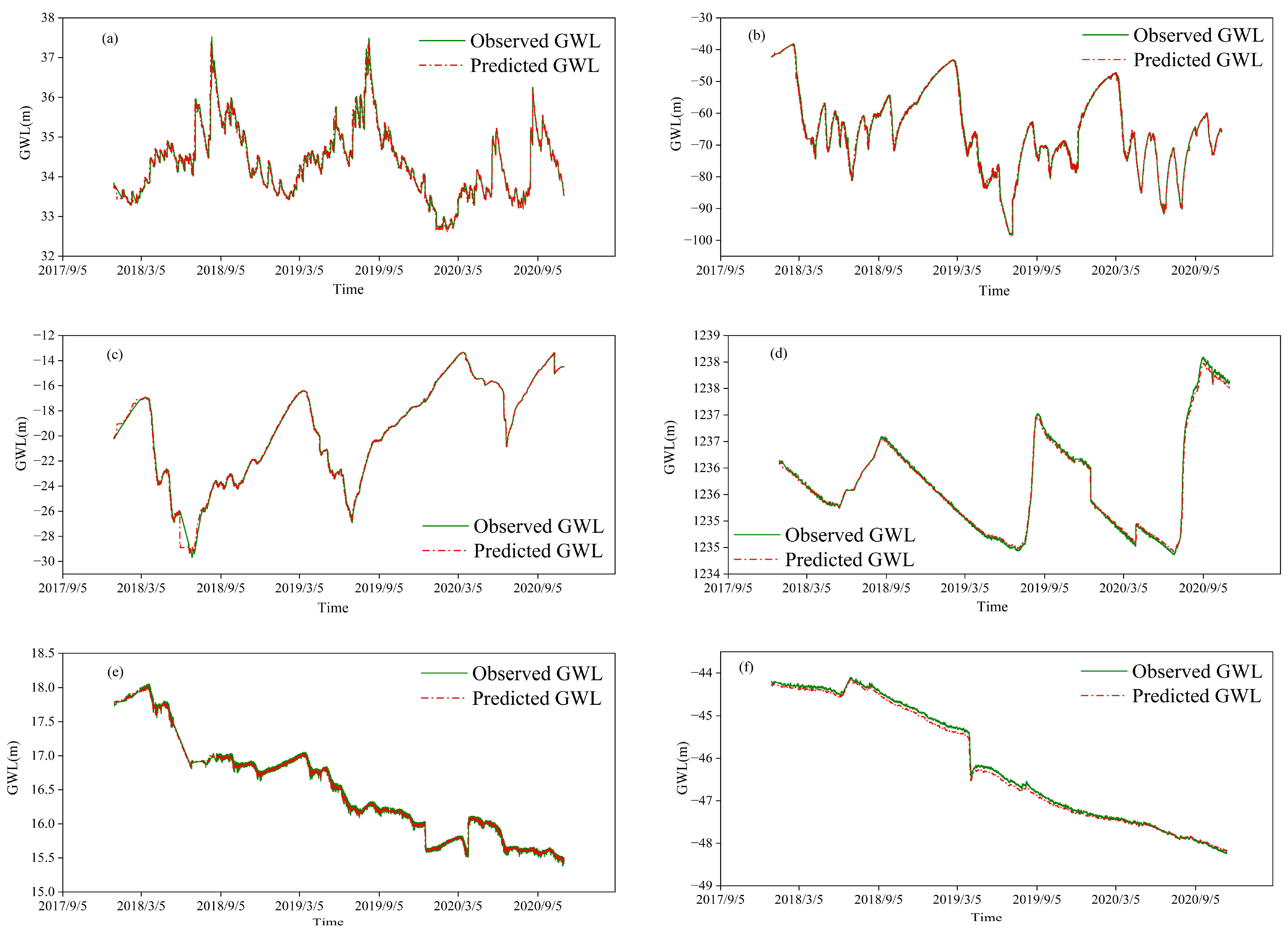
Figure 10.
Results of hourly GWL simulation (m) in six stations using the GRU model during 2018–2020 training and testing periods: (a) Huimazhai station, (b) Hongmiao station, (c) Xiliangdian station, (d) Yanmeidong station, (e) Wangduxiancheng station, and (f) XincunIIIzu station.
Figure 10.
Results of hourly GWL simulation (m) in six stations using the GRU model during 2018–2020 training and testing periods: (a) Huimazhai station, (b) Hongmiao station, (c) Xiliangdian station, (d) Yanmeidong station, (e) Wangduxiancheng station, and (f) XincunIIIzu station.

Figure 11.
Scatter diagrams of GWL simulations for each site by SVM, LSTM, MLP and GRU models: (a) Huimazhai station, (b) Hongmiao station, (c) Xiliangdian station, (d)Yanmeidong station, (e) Wangduxiancheng station, and (f) XincunIIIzu station.
Figure 11.
Scatter diagrams of GWL simulations for each site by SVM, LSTM, MLP and GRU models: (a) Huimazhai station, (b) Hongmiao station, (c) Xiliangdian station, (d)Yanmeidong station, (e) Wangduxiancheng station, and (f) XincunIIIzu station.

Figure 12.
Taylor diagrams of GWL simulations for each site by SVM, LSTM, MLP and GRU models: (a) Huimazhai station, (b) Hongmiao station, (c) Xiliangdian station, (d) Yanmeidong station, (e) Wangduxiancheng station, and (f) XincunIIIzu station.
Figure 12.
Taylor diagrams of GWL simulations for each site by SVM, LSTM, MLP and GRU models: (a) Huimazhai station, (b) Hongmiao station, (c) Xiliangdian station, (d) Yanmeidong station, (e) Wangduxiancheng station, and (f) XincunIIIzu station.


Table 1.
Data samples in the study area.
| Number | Type | Station | City | GWL | Sequence Length (Day) |
|---|---|---|---|---|---|
| 1 | dynamic fluctuations | Huimazhai | Qinhuangdao | 33.83 | 5480 |
| 2 | Hongmiao | Xingtai | 17.74 | 5480 | |
| 3 | dynamic increase | Xiliangdian | Baoding | −20.23 | 5480 |
| 4 | Yanmeidong | Baoding | 1236.14 | 5480 | |
| 5 | dynamic decrease | Wangduxiancheng | Baoding | −42.33 | 5480 |
| 6 | XincunIIIzu | Huanghua | −44.21 | 5480 |
Table 2.
Results of different performance indicators of the SVM model during the training and testing periods at each site.
Table 2.
Results of different performance indicators of the SVM model during the training and testing periods at each site.
| Station | Training | Testing | ||||
|---|---|---|---|---|---|---|
| RMSE | R2 | NSE | RMSE | R2 | NSE | |
| Huimazhai | 0.253 | 0.953 | 0.921 | 0.396 | 0.757 | 0.691 |
| Hongmiao | 2.299 | 0.98 | 0.967 | 3.823 | 0.867 | 0.804 |
| Xiliangdian | 0.298 | 0.995 | 0.994 | 0.511 | 0.915 | 0.908 |
| Yanmeidong | 0.204 | 0.998 | 0.909 | 0.193 | 0.998 | 0.984 |
| Wangduxiancheng | 0.076 | 0.992 | 0.985 | 0.071 | 0.929 | 0.808 |
| XincunIIIzu | 0.052 | 0.999 | 0.998 | 0.045 | 0.990 | 0.940 |
Table 3.
Results of the different performance indicators of LSTM model during training and testing periods at each monitoring station.
Table 3.
Results of the different performance indicators of LSTM model during training and testing periods at each monitoring station.
| Station | Training | Testing | ||||
|---|---|---|---|---|---|---|
| RMSE | R2 | NSE | RMSE | R2 | NSE | |
| Huimazhai | 0.192 | 0.955 | 0.955 | 0.263 | 0.868 | 0.864 |
| Hongmiao | 1.581 | 0.985 | 0.984 | 1.771 | 0.958 | 0.958 |
| Xiliangdian | 0.244 | 0.996 | 0.996 | 0.338 | 0.961 | 0.96 |
| Yanmeidong | 0.053 | 0.994 | 0.994 | 0.116 | 0.996 | 0.994 |
| Wangduxiancheng | 0.049 | 0.994 | 0.994 | 0.036 | 0.953 | 0.95 |
| XincunIIIzu | 0.037 | 0.999 | 0.999 | 0.028 | 0.987 | 0.976 |
Table 4.
Results of different performance indicators of the MLP model during the training and testing periods at each station.
Table 4.
Results of different performance indicators of the MLP model during the training and testing periods at each station.
| Station | Training | Testing | ||||
|---|---|---|---|---|---|---|
| RMSE | R2 | NSE | RMSE | R2 | NSE | |
| Huimazhai | 0.201 | 0.959 | 0.95 | 0.128 | 0.979 | 0.968 |
| Hongmiao | 1.419 | 0.988 | 0.987 | 0.514 | 0.997 | 0.996 |
| Xiliangdian | 0.347 | 0.999 | 0.991 | 0.295 | 0.987 | 0.969 |
| Yanmeidong | 0.033 | 0.998 | 0.998 | 0.08 | 0.998 | 0.997 |
| Wangduxiancheng | 0.041 | 0.997 | 0.996 | 0.028 | 0.969 | 0.97 |
| XincunIIIzu | 0.051 | 0.999 | 0.998 | 0.014 | 0.995 | 0.994 |
Table 5.
Results of different performance indicators of the GRU model during the training and testing periods at each station.
Table 5.
Results of different performance indicators of the GRU model during the training and testing periods at each station.
| Station | Training | Testing | ||||
|---|---|---|---|---|---|---|
| RMSE | R2 | NSE | RMSE | R2 | NSE | |
| Huimazhai | 0.182 | 0.959 | 0.959 | 0.08 | 0.988 | 0.987 |
| Hongmiao | 1.449 | 0.987 | 0.987 | 0.518 | 0.996 | 0.996 |
| Xiliangdian | 0.229 | 0.996 | 0.996 | 0.123 | 0.995 | 0.995 |
| Yanmeidong | 0.04 | 0.998 | 0.996 | 0.098 | 0.998 | 0.996 |
| Wangduxiancheng | 0.041 | 0.996 | 0.996 | 0.033 | 0.961 | 0.96 |
| XincunIIIzu | 0.081 | 0.999 | 0.996 | 0.027 | 0.995 | 0.978 |
Table 6.
Training time comparison of four models with 500 epochs.
| Model | SVM | LSTM | GRU | MLP |
|---|---|---|---|---|
| Time (min) | 1081 | 1660 | 1251 | 2694 |
Disclaimer/Publisher’s Note: The statements, opinions and data contained in all publications are solely those of the individual author(s) and contributor(s) and not of MDPI and/or the editor(s). MDPI and/or the editor(s) disclaim responsibility for any injury to people or property resulting from any ideas, methods, instructions or products referred to in the content. |
© 2023 by the authors. Licensee MDPI, Basel, Switzerland. This article is an open access article distributed under the terms and conditions of the Creative Commons Attribution (CC BY) license (https://creativecommons.org/licenses/by/4.0/).
Share and Cite
MDPI and ACS Style
Wu, Z.; Lu, C.; Sun, Q.; Lu, W.; He, X.; Qin, T.; Yan, L.; Wu, C. Predicting Groundwater Level Based on Machine Learning: A Case Study of the Hebei Plain. Water 2023, 15, 823. https://doi.org/10.3390/w15040823
AMA Style
Wu Z, Lu C, Sun Q, Lu W, He X, Qin T, Yan L, Wu C. Predicting Groundwater Level Based on Machine Learning: A Case Study of the Hebei Plain. Water. 2023; 15(4):823. https://doi.org/10.3390/w15040823
Chicago/Turabian StyleWu, Zhenjiang, Chuiyu Lu, Qingyan Sun, Wen Lu, Xin He, Tao Qin, Lingjia Yan, and Chu Wu. 2023. "Predicting Groundwater Level Based on Machine Learning: A Case Study of the Hebei Plain" Water 15, no. 4: 823. https://doi.org/10.3390/w15040823
Note that from the first issue of 2016, this journal uses article numbers instead of page numbers. See further details here.