
Rainfall Prediction Rate in Saudi Arabia Using Improved Machine Learning Techniques


1
Department of Computer Engineering, College of Computer and Information Sciences, Majmaah University, Majmaah 11952, Saudi Arabia
2
Department of Information System, College of Computer and Information Sciences, Majmaah University, Majmaah 11952, Saudi Arabia
*
Author to whom correspondence should be addressed.
Water 2023, 15(4), 826; https://doi.org/10.3390/w15040826
Submission received: 4 January 2023
/
Revised: 15 February 2023
/
Accepted: 15 February 2023
/
Published: 20 February 2023
(This article belongs to the Special Issue Understanding Circular Economy Complexities and the Climate–Water–Food–Energy Nexus in an SDG Framework: Interactions and Alternatives for Decision Making)
Abstract
:Every farmer requires access to rainfall prediction (RP) to continue their exploration of harvest yield. The proper use of water assets, the successful collection of water, and the successful pre-growth of water construction all depend on an accurate assessment of rainfall. The prediction of heavy rain and the provision of information regarding natural catastrophes are two of the most challenging factors in this regard. In the twentieth century, RP was the most methodically and technically complicated issue worldwide. Weather prediction may be used to calculate and analyse the behaviour of weather with unique features and to determine rainfall patterns at an exact locale. To this end, a variety of methodologies have been used to determine the rainfall intensity in Saudi Arabia. The classification methods of data mining (DM) approaches that estimate rainfall both numerically and categorically can be used to achieve RP. This study, which used DM approaches, achieved greater accuracy in RP than conventional statistical methods. This study was conducted to test the efficacy of several machine learning (ML) approaches for forecasting rainfall, utilising southern Saudi Arabia’s historical weather data obtained from the live database that comprises various meteorological data variables. Accurate crop yield predictions are crucial and would undoubtedly assist farmers. While engineers have developed analysis systems whose performance relies on several connected factors, these methods are seldom used despite their potential for precise crop yield forecasts. For this reason, agricultural forecasting should make use of these methods. The impact of drought on crop yield can be difficult to forecast and there is a need for careful preparation regarding crop choice, planting window, harvest motive, and storage space. In this study, the relevant characteristics required to predict precipitation were identified and the ML approach utilised is an innovative classification method that can be used determine whether the predicted rainfall will be regular or heavy. The outcomes of several different methodologies, including accuracy, error, recall, F-measure, RMSE, and MAE, are used to evaluate the performance metrics. Based on this evaluation, it is determined that DT provides the highest level of accuracy. The accuracy of the Function Fitting Artificial Neural Network classifier (FFANN) is 96.1%, which is higher than that of any of the other classifiers currently used in the rainfall database.
1. Introduction
Knowledge can be analysed from various angles and then distilled into usable data in a process known as data mining [1]. Users are able to obtain information from different dimensions and technically summarise attribute correlations via data mining. To provide accurate forecasts, the method gleans relevant information from the observable characteristics of current and historical weather data. This article offers an original forecasting model to investigate the general climatic changes and the factors that cause severe weather occurrences in Saudi Arabia.
The purpose of this approach is to compile relevant data from the database and implement a subset of climatic variables [2], which significantly improves accuracy. The models created with the help of data mining methods are broken down into several steps so that the meteorological datasets and the algorithms can be evaluated. The following classifiers are drawn from several data mining strategies and are used in the proposed method: the multiple linear regression approach, the decision tree method, the k-nearest neighbour [3] method, the support vector machine algorithm, the artificial neural network methodology, and the random forest algorithm.
Experiments using advanced statistical prediction methods for short-range, medium-range, and long-range forecasting in regular monsoon rainfall and extreme rainfall events have been used in Saudi Arabia, and are utilised by the Saudi Arabian Metrological Department [4] to make daily forecasts. High-resolution datasets are generated about the climate, including rainfall characteristics and temperature datasets. Researchers worldwide use these datasets effectively.
One of the goals of this research is to develop objective criteria for predicting monsoons over the southern region of Saudi Arabia and to effectively follow the Saudi Arabian summer monsoons [5]. For operational purposes, the Saudi Arabian Meteorological Department uses several factors to study severe climatic situations such as solid precipitation, monsoon droughts, and heatwaves, and to understand the physical model processes.
Utilising observations and regional climate models, we have created a high-resolution ground surface data collection method for hydrological applications. This study focuses on the function of monsoon surface processes. The active and break periods of the Saudi Arabian monsoon, including description parameters and processes, have been extensively cited and are utilised by academics in their research [6]. Using modern datasets gathered from satellites, researchers investigate the three-dimensional cloud patterns and the instability of such structures over the monsoon region and study space–radiation interactions and weather radiative pressure over the monsoon zone using many satellite datasets, as well as observing cloud radiation input throughout the Asian Monsoon region [7]. Multivariate information helps depict a wide variety of models and processes. Using multivariate data analysis techniques, one may visualise variables and reactions, uncover the connection between all components and reactions, and ultimately extract helpful information from multivariate data [7]. Multivariate data analysis provides insights into the current and future demands to help with problem solving and may be used better to comprehend the characteristics of various frameworks and forms.
The purpose of linear regression is to create a connection between a response variable (the dependent variable) and a set of explanatory factors (the independent variables) [8]. Factor Analysis (FA) examines the influence of the common variance of the independent variables under investigation on the dependent variable. Canonical correlation (CC) shows how significantly the independent variables are associated with the explanatory variable, regardless of whether they are related. Dimensionality reduction and visualisation of the main factors affecting crop yield (CY) are two more applications of the diagnostic model known as principal component analysis (PCA).
For the evaluation and interpretation of the predictability of the Saudi Arabian Monsoon inside climate models, the Climatology Section, which is a component of the Regional Meteorological Centre (RMC), Ref. [8] is the primary institution that handles all of the Qassim region’s climatic and meteorological operations linked to the area.
There are many different kinds of data, such as hourly-based, daily, monthly, and annual rainfall data, as well as divisional station-based hourly, daily, and averaged monthly temperature data, averaged maximum and minimum temperatures, and extreme temperature forecasting. The combination of water vapor and air measured hourly, daily, and monthly is referred to as relative humidity. The surface wind speed, direction of the wind, and amount of sunlight are also measured hourly. Additionally, the pressure at the station level and the pressure at mean sea level are recorded on an hourly, daily, and monthly basis. The volume and types of clouds [9] are recorded eight times daily. The incidence of other meteorological phenomena, such as thunderstorms, visibility, and heavy spells, are also documented. Various weather reports, including those on storms, wind rode graphs, and severe rainfall, are also available to researchers.
2. Related Study
According to [10], machine learning approaches are frequently employed in the process of making predictions about financial time series data. The suggested model detects the changes in financial market prices with near precision, and money can be made merely because these forecasts are sufficiently correct. Researchers have attempted to debunk the general theory of financial economists, which states that predictability and successful trading in financial markets cannot be achieved accurately, by providing evidence that contradicts this work. The model’s predictions regarding financial markets are more accurate than the most advanced econometric approaches. The authors concluded that financial forecasting is affected by factors such as the maturity of the market, the methods used for the prediction, the scope for which it develops forecasting, the methodology used to access the model, and the simulation-based model training. The investigative study demonstrates that sophisticated prediction models may be of considerable use in attempting to forecast the changes in price that will occur in financial markets.
According to [11], a machine learning system is able to carry out superior forecasting in the context of weather prediction. The ML model is able to forecast by making use of satellite-based datasets that are complicated and comprise rainfall retrieval variables. The improvements in parallel computing with machine learning algorithms are particularly beneficial in training the dataset as well as in anticipating future trends, and these are the reasons behind adopting machine learning technology in real-time practical applications. In this study, the researchers analysed the MSG SEVIRI data from Germany by making use of four different machine learning algorithms, namely, support vector machines, neural networks (NNET), averaged neural networks (AVNNET), and random forests (RF), for the purpose of determining the rainfall rate and identifying the types of precipitation. Within the scope of this research, consideration was given to the satellite-based predictor variables of cloud water path, cloud phase, cloud temperature, and cloud height. According to the findings of the researchers, NNET and AVNNET perform much better than the other models. The authors conclude that additional study into the provision of appropriate and precise rainfall forecasting is urgently required.
The authors of [12] presented a new sort of forecasting model that utilises three out of the four models mentioned above. In [12], a survey was conducted regarding the extreme rainfall event that occurred over the north coastal region of Saudi Arabia, which included the city of Qassim. According to their findings, the Qassim region was hit by three separate bouts of heavy rain in the following time periods: 8th to 9th November, 16th to 17th November, and 30th November to 1st December 2015. The study was conducted on the basis of the observation of an anomaly in the global land surface air temperature, which was related to the yearly variable rainfall of Saudi Arabia’s summer monsoon. The overarching circumstances of these three significant rainfall occurrences during the previous 52 weeks are as follows. The dramatic occurrences took place as a result of a significant depression that occurred close to the south-west corner of the Bay of Bengal and was accompanied by cyclonic circulation that stretched to the middle troposphere over the south-east region of Saudi Arabia. The authors of [13] suggested a model that is based on positive correlation coefficients of independent meteorological indices. These parameters include surface temperature and air temperature. Extreme rainfall activities, floods, and natural disasters around the coast of Saudi Arabia were used to help the writers identify the criteria.
The research in [14] contributed to the development of a prediction method for estimating future rice output. For the purpose of the experimental study, the researchers made use of a dataset that relates to an area of Bangladesh. Climatic factors such as wind speed, temperature, and rainfall have a significant impact on the location that was chosen for this research. The researchers projected the yield of crops by making use of machine learning algorithms, and by utilising the model, the authors tested its performance on unknown climatic factors that may cause changes in the production of crops. The initial step in training the model is to establish a connection between historical ecological patterns and agricultural output rates.
In [15], a model was developed to calculate the price of stocks using multiple classifiers. The results compared the individual classifier techniques such as logistic regression, KNN, support vector machine, and neural networks with those of the ensemble models such as random forest, AdaBoost, and kernel factory. The research gathered 5767 records of European businesses for the purpose of experimental examination. The performance measure was assessed with the assistance of 53 characteristic curves, and the findings revealed that random forest ensemble models demonstrated high accuracy in comparison to other classification models.
For the purpose of landslide susceptibility modelling, Ref. [16] suggested prediction approaches that evaluate statistical methodologies in conjunction with data mining techniques. The geotechnical information that is mapped into areas prone to landslides is employed in the development of models based on the actual world. The experimental research was carried out in the three distinct areas that make up the province of Lower Austria. A modular model provided by [17] consists of many sub-processes that are further separated into local expert models. The modular model that was developed using the training data was divided into a hard split and a soft split. When datasets overlap, this technique is referred to as soft splitting, and the prediction is made using the weighted average of each local model. During the hard-splitting process, the dataset will not be overlapped, and prediction will be conducted based on a single local model. The ensemble model integrates numerous different models.
Case-based reasoning is a paradigm for the creation of expert systems that recycle previously implemented solutions to address new challenges. The first strategy makes use of CBR to save K examples that are similar to one another in order to solve the motion planning issue by combining the various answers into a set. After that, it makes its selections for the final answer based on a heuristic function, choosing from among these potential options. The retained K comparable examples are used in a different manner by the second technique. It does this by using those solutions to construct a graph that can be searched using conventional graph search techniques.
The findings demonstrate the viability of such techniques with regard to the quality of the solutions and the success rate in comparison to various experience-based algorithms. Because of its use for CBR systems, new research avenues are developed for the construction of systems that are capable of solving NP problems only on the basis of retained experiences.
In their study, Ref. [18] describe a novel approach to learning-based path planning. It uses a graph-based route planner that was recently suggested as a “training expert” and imitation learning. In order to achieve exploratory behaviour comparable to that of the training expert with a more than an order of magnitude reduction in computational cost, the algorithm only uses a short window of range data sampled from the onboard LiDAR. Concurrently, the need to maintain a consistent and online reconstructed map of the environment is relaxed as a result of this. In the context of the autonomous exploration of underground mines, the taught route planning strategy is subjected to intensive testing both virtually and in the form of field trials, where it is reviewed in great detail.
The accuracy of a forecast [19] is strongly influenced by the qualities that have the greatest potential for information acquisition and the most comprehensive sets of data. It was also discovered via the review of the relevant literature that the performance of the algorithm is fully dependent on the quality of the data that is readily accessible. The entropy measurements guarantee that the data used for the training and testing of the data mining method are of a high quality. It should also be mentioned that the vast majority of data mining approaches and hybrid techniques employ conventional data-cleaning methods and normalisation processes, both of which are used in this study. It is also stated that standard error measures such as SSE and RMSE [20] have been used to compare and assess the implemented models. This information was gleaned from the research of the relevant literature. This study was executed utilising a wide variety of data mining methods, and the analysis that was completed was based on the accuracy and execution time. This information was gleaned from the research of the relevant literature [21]. The study work that was suggested has been executed utilising a wide variety of data mining methods, and the analysis that was completed was based on accuracy and execution time.
3. Methodology and Data Description
The datasets utilised in the study can be obtained for free from the internet; they were gathered from the Saudi Arabian Metrological Department website. The dataset represents rainfall information compiled from the more comprehensive weather information for Saudi Arabia. The NCEP/NCAR Reanalysis data collection incorporates observations and a numerical weather prediction (NWP) model, providing information about the Earth’s atmosphere. These data are continually updated and reviewed by a large number of scholars all around the globe.
3.1. Weather Features
The following list provides the characteristics that may be derived from the database for the research efforts that have been suggested. The study team carefully considered various pertinent aspects to develop trustworthy data mining strategies for prediction. Evaporation, terrain characteristics, sea level height, relative humidity, specific humidity, pressure, temperature, sea surface temperature, sea level pressure, precipitable water, evaporation, geopotential height, cloud cover, wind speed, dew point, zonal wind, meridional wind, sunshine, and dew point temperature are the features that are taken into consideration.
- Temperature: The atmosphere’s temperature indicates the temperature of the various layers of the Earth’s atmosphere. The factors determining the temperature are the amount of incoming solar radiation, precipitation, and altitude. The energy density component of the sun’s air temperature changed from day to day, month to month, season to season, and even latitude to latitude. The sun sends forth short waves of energy, which are absorbed by the Earth, which then emits long waves. The quantity of heat energy absorbed by the Earth and the amount it emits are evaluated against one another on a comparative scale.
- Humidity: Humidity refers to water vapor in the air. The current temperature affects the relative humidity that is present. In some conditions, such as when the water evaporation rate is very high, the relative humidity will be treated as if it were the absolute value.
- Wind flow: The movement of gases on a broad scale is called wind. Wind is the driving force behind air movement on Earth and is caused by differences in atmospheric pressure. When the pressure is measured, there is a movement of air from the high-pressure to the low-pressure level. Wind speed is affected by a variety of variables and causes, and it can be measured using several different scales. The pressure curve, jet streams, Rossby waves, and local weather are some examples of these. During periods of air and pressure disturbance across surfaces, wind speed and direction are connected and interdependent properties.
- Water level: The depth of the water level in the atmospheric column is referred to as the water level. The complete water content of the atmospheric column condenses to become rain. The total amount of water vapour in the air is estimated as the cross-sectional area of a vertical column and measured at a range that is often expressed as the height of the water column (in millimetres or centimetres).
- Solar radiation: This is a kind of atmospheric parameter that may be measured on a daily basis or on a yearly basis from a particular site within a region.
- Evaporation: Evaporation is a process that takes place in the atmosphere and involves the transformation of water from its liquid state into a gas or vapour. The amount of water that is lost by evaporation from a pan is measured in inches of depth as the unit of measurement.
- Dew point: This is the temperature at which water droplets begin to condense and create a dew. When the ambient temperature shifts in response to changes in pressure and humidity, the beginning of this process is initiated.
- Sea surface temperature: The temperature of the sea surface is the water temperature that is most closely related to the surface of the ocean. The precise definition of the surface might change depending on the methodology used to measure it. The unit of measurement ranges from 1 millimetre (0.04 in) to 20 metres (70 ft) below the surface of the water.
- Sea level pressure (SLP): The mean sea level pressure is an average of the atmospheric pressure measured at the mean sea level. The standard level of pressure is an atmospheric pressure that is often discussed in weather forecasts.
- Relative humidity: Relative humidity is the ratio of the amount of water vapour in the air to the total mass of the air. The value of the measurement is given in terms of grammes of vapour per kilogramme of air.
- Omega: The word omega refers to the vertical motion that occurs in the atmosphere. If the weather prediction chart indicates that there is a high value of omega or a strong omega field, this indicates that the omega value is associated with upward vertical motion (UVV) in the atmosphere. Severe episodes of heavy rain, thunderstorms, and other types of precipitation are measured based on the upward vertical motion.
- Geo potential height: The geo potential height, also known as the geo potential altitude, is a vertical coordinate that is referenced to the mean sea level of the Earth. It is an adjustment to the geometric height, which is the altitude above the mean sea level, that takes into account how gravity varies with both latitude and altitude.
- Zonal wind: This is component of a wind that blows along a certain latitude parallel.
- Meridional wind: The meridional wind, sometimes known simply as wind, is a component that, in contrast to zonal wind, exists in addition to the local meridian. The horizontal coordinate system is established locally with the X-axis pointing eastward and the Y-axis pointing northward. Next, the meridional wind is described as positive if the wind is coming from the south, and it is characterised as negative if the wind is coming from the north.
Input climate complex presents a global surface summary of day data, version 7, for over 9000 worldwide stations. As per the World Meteorological Organization (WMO) World Weather Watch Program, the data summaries provided here are exchanged among the nations. The summaries and products of different countries are made available, which are intended for free, open access, and unrestricted use in research and development, education, and other non-commercial activities. The following is a description of the global surface summary produced. The current daily summary data are normally available 1–2 days after the date and time of the observations. The daily elements included in the dataset are as follows:
- (i)
- Mean temperature, max., min. (0.1 Fahrenheit).
- (ii)
- Mean dew point (0.1 Fahrenheit) (DP).
- (iii)
- Mean sea level pressure (0.1 mb) (SLP).
- (iv)
- Mean station pressure (0.1 mb) (SP).
- (v)
- Mean visibility (0.1 miles).
- (vi)
- Mean wind speed (0.1 knots) (WS).
- (vii)
- Maximum sustained wind speed (0.1 knots) (SWP).
- (viii)
- Maximum wind gust (0.1 knots) (WG).
- (ix)
- Precipitation amount (0.01 inches) (x).
- (x)
- Snow depth (0.1 inches).
The data were processed in order to remove any unexpected values. This was accomplished via the use of personal experience. Only values such as 7777 and 5555 were omitted as these figures were uncommon and were ultimately superseded by an average value for rainfall. After determining the highest and lowest possible temperatures and amounts of precipitation for each individual year, the next step was to calculate the yearly averages for those parameters over a period of thirty years.
The vast majority of the characteristics related to the open-source data were found on the websites of different regional meteorological centres, the Saudi Arabian Meteorological Department, open-source data from NOAA/NECP, reliable internet sources, and the website of the Qassim region regional meteorological centre. Following the data gathering phase were the data cleaning methods, data selection methods, data transformation techniques, and data mining stages. The pre-processing removes any ambiguity that may arise during the data mining process. The prediction algorithms contain established procedures for noise control and data imputation. In order to arrive at a conclusion, the gathered datasets are subjected to a variety of pre-processing procedures.
3.2. Data Cleaning
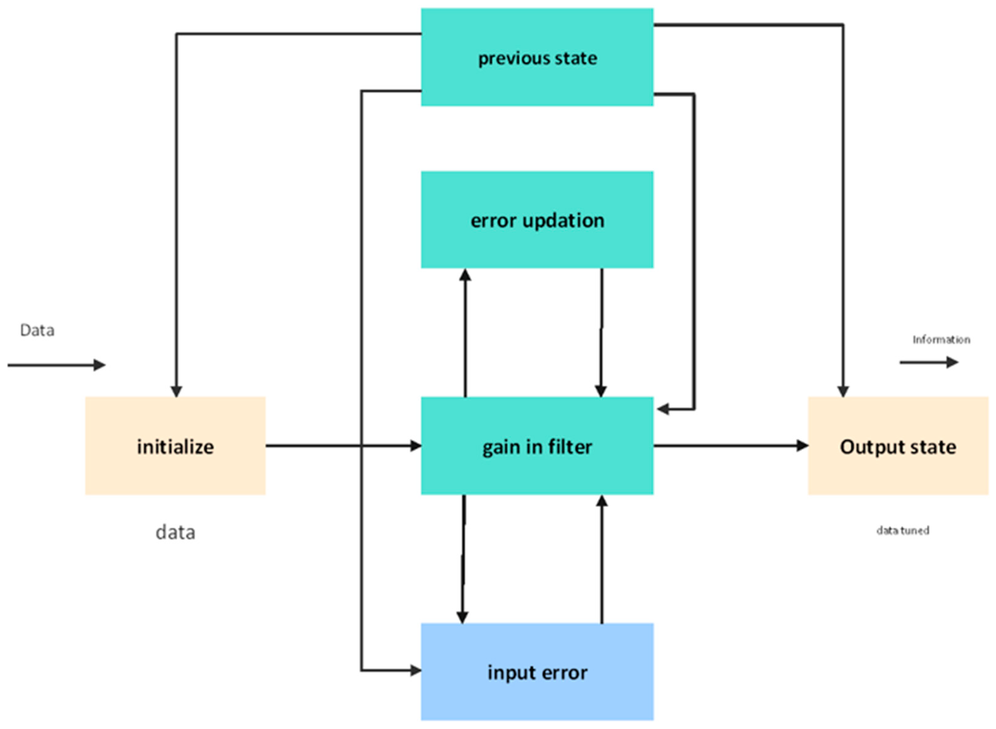
The goal of the data cleaning process is to determine the causes of the problems found in the dataset and to devise methods that can be used to prevent errors from occurring in the data collection process in the future. It enhances the overall quality of the data while at the same time reducing the amount of incoherence that is present in the sample. The discipline of data mining makes frequent use of the pre-processing approach discussed in this article. At this point, the architecture of a consistent data model is constructed in order to handle missing data in an efficient way. This is one of the steps in the process. The algorithm known as the Kalman filter is used when there are missing or incorrect values that need to be replaced. The Kalman filter is a simple method that can accurately forecast the current value of a variable by analysing data from the past and comparing it to the current value of the variable. The Kalman gain K is used by the Kalman filter method, which works to continually update the values that are being delivered to the projected state. The components that comprise the Kalman filter algorithm are shown in Figure 1.
Assume a temperature with noise at time t. The Kalman filter algorithm estimates the temperature and compares it with the current temperature to decide the predicted temperature at time . Now the KF filter must remove the noise.
Step 1. Compute the predicted temperature from the previously estimated value using Equation :
where is the internally predicted temperature, is the state transition, is the control matrix, is the previous temperature at time , and is the control vector.
Step 2. Uncertainty in the internally predicted temperature is determined by a covariance factor, which is updated using Equation :
where is the state transition matrix, is the transpose matrix, is the old value of covariance, and is the estimated error.
Step 3. Kalman gain is updated using Equation , as follows:
where is the observation matrix, is the transpose matrix, and is the estimated error in the measurements.
Step 4. Assume the current temperature at time is . Then, the predicted temperature is calculated using Equation :
Step 5. The covariance factor is updated for the next iteration using Equation :
As a result, the Kalman filter method will replace any missing data or erroneous values. Following the completion of the data cleaning process, the experimental data were changed into target data, a structured model for prediction. The vast majority of the data accessible on the internet could be of better quality. There are many different software solutions available for data transformation, and their primary purpose is to offer data cleaning procedures for raw data.
3.3. Classification
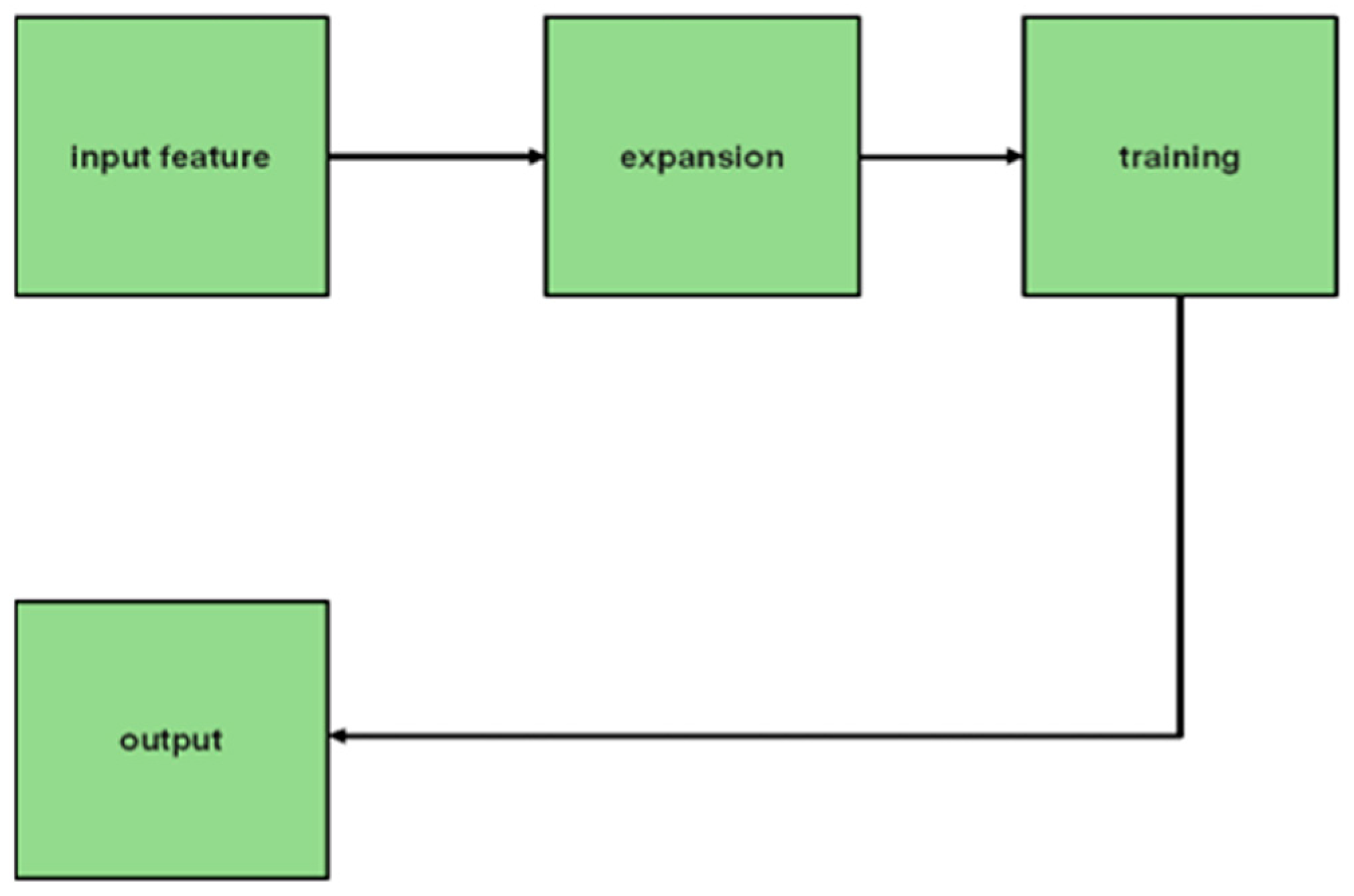
In our proposed link artificial neural network (LANN), in order to estimate the software development effort, we determine the network architecture parameters according to the characteristics. The general structure of the functional link artificial neural network is shown in Figure 1. (TL—temperature low, TM—temperature medium, TH—temperature high, DL—dew low, DM—dew medium, DH—dew high, VL—visibility low, VH—visibility high, VM—visibility medium, —precipitation).
3.4. Attribute Selection
The dataset’s accuracy and precision are both improved by the use of normalization procedures. In order to improve the generalization and prediction, many kinds of normalizing approaches, such as rescaling, standardization procedures, and rescaling to unit length, are used in the processing of meteorological datasets. There are many scales that are used to measure the values of the weather data. Integer types, floating point values, Boolean data types, and range values are several ways in which attributes may be measured. During the normalization process, the actual range values are rescaled to unit scale values, and the minimum and maximum range values are converted into standard values for these ranges. The purpose of standardization is to reduce the number of errors that occur by establishing a common range of data compiled from a variety of data sources. The training of weather prediction models based on clustering or classification is made more effective by standardization.
The normalizations utilized in the model used to forecast the weather are derived from nonlinear transformations. When the range of variables is constrained to fall within a small number of minimum and maximum values, the accuracy of the results improves to 71. When conducting sigmoidal normalization, the ranges 0 to 1 (or −1 to +1) are the ones that are allocated. A nonlinear sigmoidal normalization was included in the weather forecasting model. The methods of normalization based on the median were used in order to standardize the input values of the weather data. This normalization is applicable to datasets that disperse data samples across inputs, such as those dealing with the atmosphere. The suggested model for weather forecasting incorporates the following three data standardization techniques that are employed in the classification system. These methods are developed to work with binary and multiclass datasets.
(a) Min–Max Normalization
The min–max approach of normalization implements the usage of linear regression in order to modify the meteorological data and normalize the samples. The linkages between the true atmospheric input and the normalized new values are preserved by the min–max normalization technique. When procedures detect a deviation in standardized values from the initial dataset, this indicates that an error has been made. The use of this technology ensures that the normalized input values that fall within a certain range will be severely confined. The min–max method of normalizing changes X0 to Xn, which indicates that the value falls within the allowed range.
Here, is the normalised value of , is a current value of , and and are the minimum and maximum of the input data, respectively, followed by the detailed functional link artificial neural network architecture in Figure 2.
The classifier has four hidden layers: the sequence input layer, fully connected layer, softmax layer, and classification output layer. In this portion of the article, we offer an innovative hybrid model consisting of a multilayer artificial neural network for the goal of obtaining an accurate evaluation of the expenses associated with software development. It is widely held that artificial neural networks, on account of their capacities for self-learning, modelling complicated nonlinear connections, swiftness, and fault tolerance against noise, are among the most effective tools for providing solutions to issues pertaining to prediction.
In this case, we use a multilayer layer artificial neural network as our core architecture for the purpose of developing accurate estimates of the costs associated with software development. The Firefly algorithm is utilized as the training algorithm for this network due to its multimodal optimization capability.
Numerous architectures of neural networks have been established in the past for a variety of purposes, and there are many of these architectures. The architectural configuration of a neural network is dependent on both the design of the network and the performance limitations it sets. A variety of factors are used in an artificial neural network, such as: (1) an input layer and the number of nodes included inside it; (2) the total number of hidden layers and the total number of nodes in each hidden layer; (3) the parameters of the training procedure; and (4) the weights that are assigned to each communication channel present between neuronal connections in the research that we have suggested. In our case, we use 20 different numbers of nodes as inputs. These numbers represent 15 different effort multipliers and five different scale factors. In the network that we have suggested, we set the learning rate to 0.1 and the bias parameter, “b”, to a value of 1.00.
In addition, the identity activation function is employed in our developed network in order to determine the desired output from the network. After obtaining the results as an output from the multilayer layer artificial neural network, they are repeatedly passed to the Firefly algorithm to train the network, and the output, if it is discovered to be optimal, becomes the solution as a desired criterion of estimation. If the output is not found to be optimal, the process of training is continued until the solution is found.
Algorithm A1: Pseudo code of proposed forecasting model (Appendix A).
The J4.8 model performs a heuristic division to maximize the information gain. The information gain ratio enables the identification of the best attribute with the power of discrimination between classes. The information gain is measured using Shannon entropy. The entropy is expressed in Equation :
where D specifies the datasets, and specifies the proportion of dataset D belonging to class . The information gain of of attribute provided the collection of , as given in Equation :
where Values(A) is the set of possible values for , and is the subset of for which has value (i.e., ). The information gain ratio is a measure defined from gain and split information.
where Split Information(D, A) is defined in Equation .
The maximum information gain variable is omega at , which indicates the upward vertical movement of the atmosphere at coordinate . As predicted, the coordinate is as near to the disaster zone as the limited spatial resolution of the gridded data permits.
4. Experimental Results
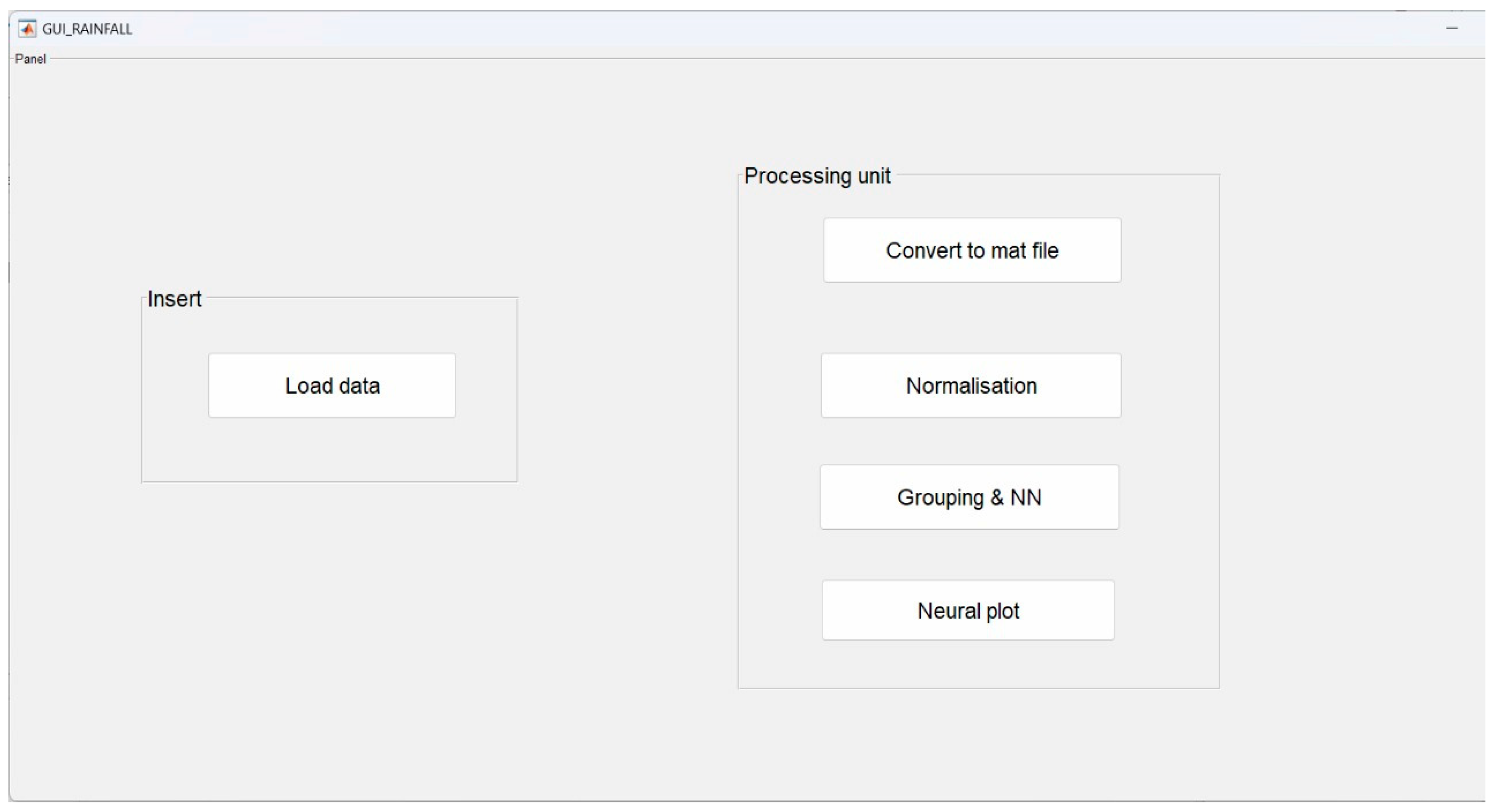
The FFANN technique was designed with the Hadoop–MapReduce framework for seasonal rainfall forecasting, with the case study region as Saudi Arabia and the dataset used in developing the forecasting model. The proposed model was designed and implemented using MATLAB. The performance of the model was assessed and compared with the existing strategies in terms of R-square, MAPE, and RMSE. The input climate data, outcomes, screenshots, and charts were produced at the end of each model. This section describes the execution of the FFANN model for rainfall prediction. Figure 4 shows the GUI window of proposed work implementation.
The model was implemented using R-Tool on a Windows 7 operating system with a and hard disk. The accuracy of the model was calculated using the Percentage Forecast Error (PFE) and value. is a statistical measure of how close the data are to the fitted regression line and is computed by Equation (13):
where SSE is the sum of the squared errors, SST is the sum of the squared total, is the number of observations, and is the regression coefficients. The higher value of indicates that the model is good for prediction. The percentage forecast error of the method is measured by Equation (14):
where is the actual value for weather forecast and is the forecast value of the crop yield. The lower value of the PE indicates better prediction accuracy.
The results of the two hidden layers are shown in Table 1 with an LR value of 0.50. The best results were achieved for a number of neurons using the first layer’s value of 30 and the second layer’s value of 60, both of which had an R-square value of 0.94.
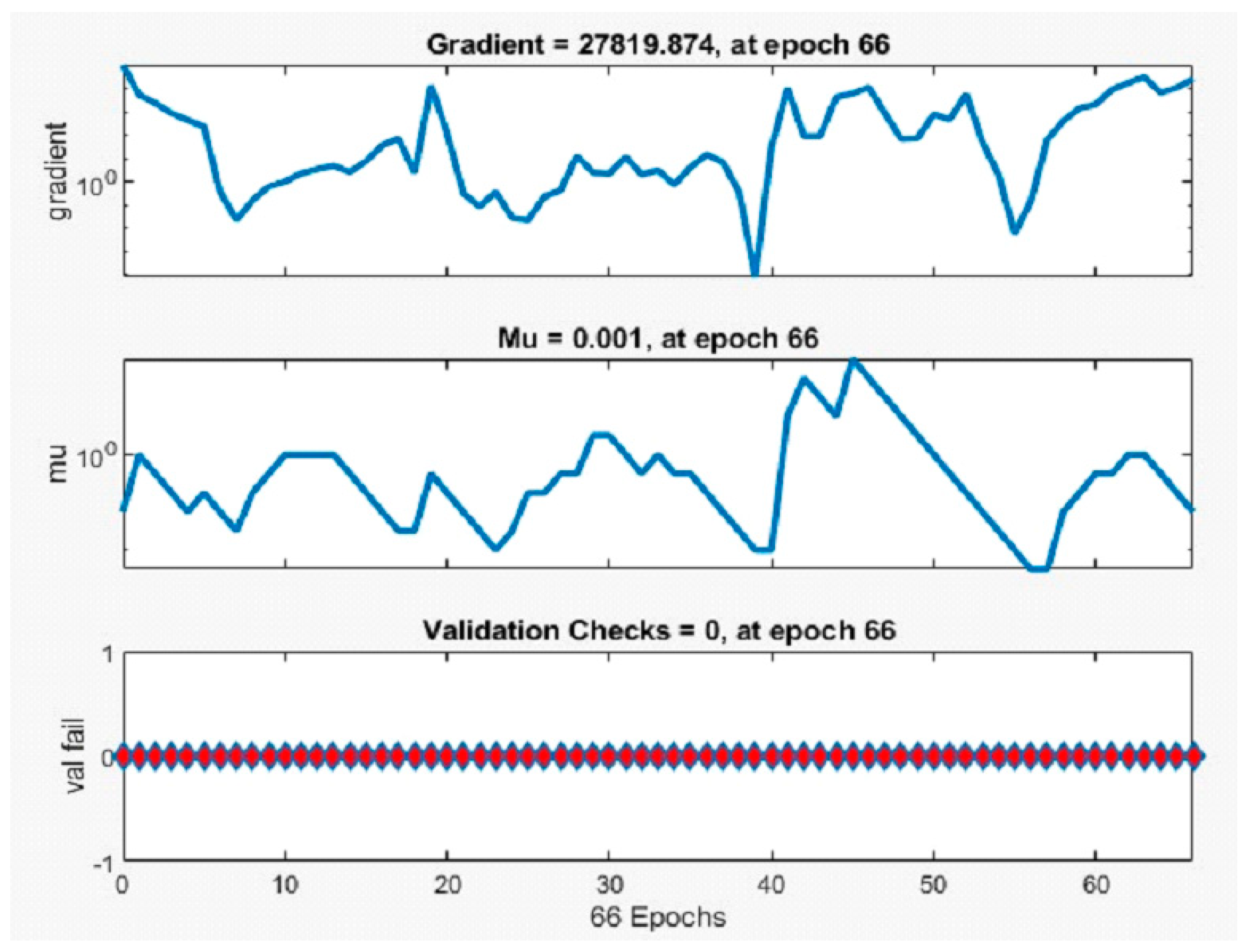
The FFANN model with the following combination yields the best result of 0.97 (R-square) as two hidden layers and the number of neurons for the first layer is 40 and the number of neurons for the second layer is 80 with LR 0.25. The results are shown in Table 2. Figure 5 shows the training epochs of the proposed work.
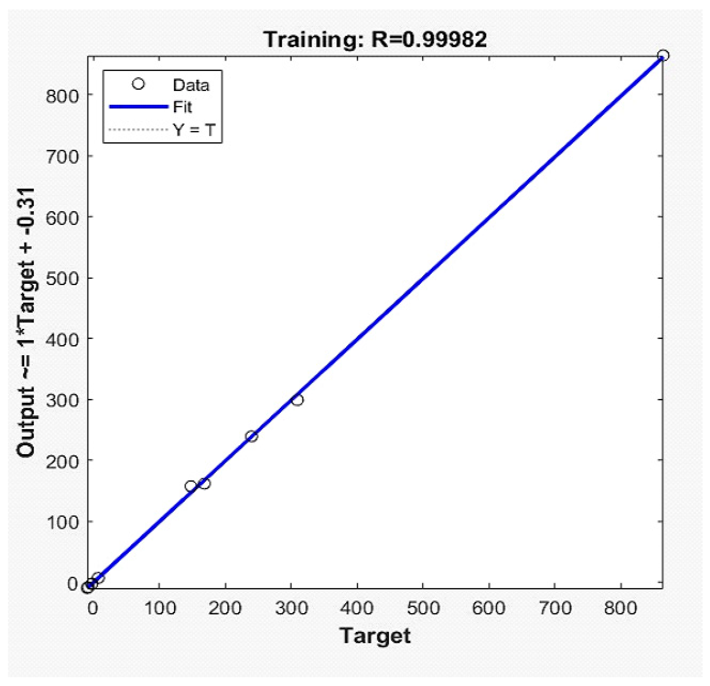
Figure 6 shows the neural network testing phase. It is possible to calculate the F-statistic for more than two different groups. In this scenario, at least one of the classes corresponding to the alternative hypothesis has to have a distribution that is distinct from the others. The scores from the t-test and the F-test were transformed into probabilities, referred to as the p-value. A p-value is the probability that, under the assumption of the null hypothesis, one would see a t-statistic (or F-statistic) that is larger than the one derived from the data. The level of statistical significance may be determined by looking at the p-value. Both the test and the datasets make the assumption that normal distribution applies (Figure 7). If the dataset that is available to analyze is rather limited, non-parametric alternatives to these tests, such as the Wilcoxon test, the Kruskal–Walli’s test, or a permutation procedure, may be more appropriate.
The findings of the FFANN illustrate the essential factors that played a crucial role during the heavy rainfall that occurred in the Qassim region in 2015. The extreme rainfall was caused by the vertical transport of the moisture that was transported from the ocean by sustained easterly winds. The model was effective as a predictor in that it was able to accurately anticipate all of the severe rainfall events that took place over the course of the evaluation years.
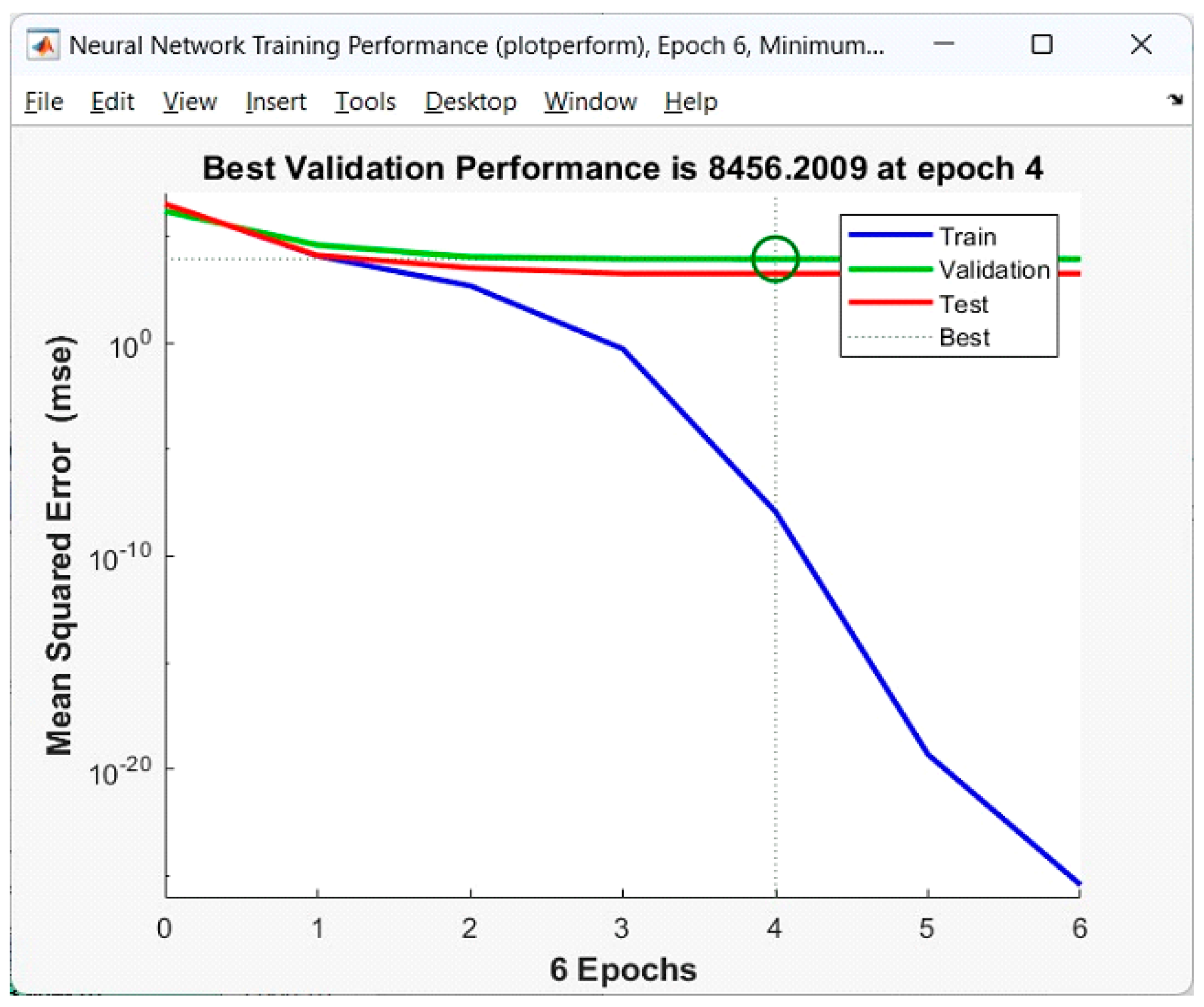
Agriculture, the planning and building industry, and water resource management may all benefit from an early warning system that is provided by the ability to predict high rainfall occurrences. Being able to accurately forecast how much rain will fall gives farmers an advantage in terms of crop planning and selection. The farmer can better plan the sort of crops that will grow, whether short-term or long-term yields, thanks to accurate predictions of the geographical and temporal distribution of rainfall events. FFANN may be used in medical applications, financial analysis, applications related to molecular biology, and applications related to object identification, as well as in remote sensing, such as satellite launching vehicles, orbit tracking, and radar monitoring. Figure 8 shows the validation rate.
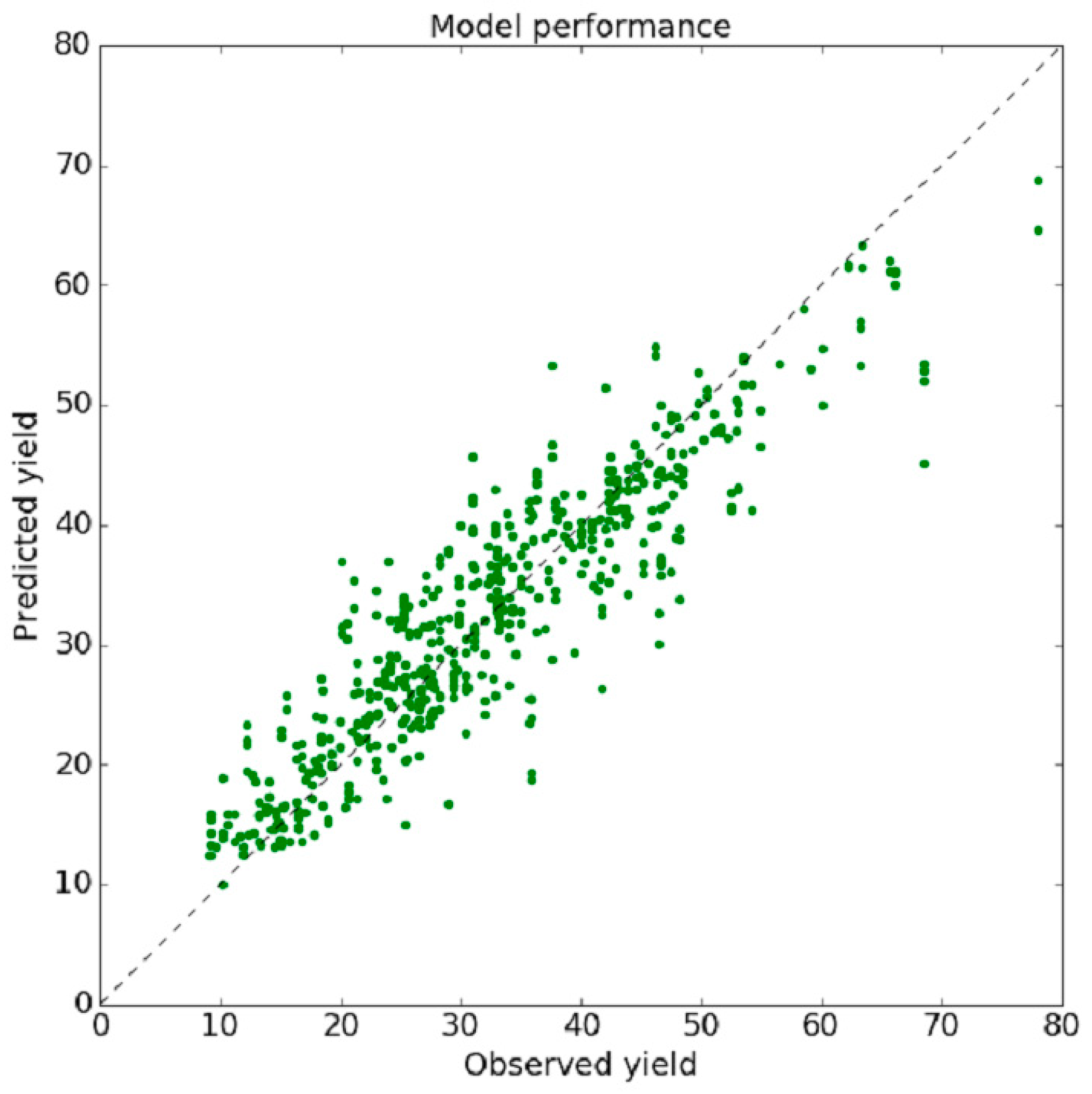
The common variance among the explanatory variables studied that affects crop yield may be calculated using factor analysis (FA). Factor analysis is used to determine the structure of a dataset and the connections between its elements. Crop yield is the response variable while minimum support price, consumer price index, food price index, area under the curve, and adjusted R-squared are the explanatory factors evaluated. In factor analysis, the explanatory variables are reduced to elements is shown in Figure 9.
Factor analysis is a method for reducing the number of components to their underlying relationships and discovering patterns in the original data with little information loss. MSP, CPI, FPI, AUC, and AR are the metrics used in this evaluation. MATLAB is used to analyze FA. FA is used to create a model fit for the cereals rice, maize, and gram once the data has been imported. If one latent component is found to have a very positive weight on all five of the observable variables, this would be reflected in the estimated loading. If the value of factor loading is high, it indicates that the factors have a strong relationship with the dependent variable. With a particular variance equal to 1, we may infer that the components are highly correlated with one another. The goal of factor derivation and overall fit analysis is to determine the strategy for factor extraction, in addition to selecting the number of factors that will be utilized to model the underlying observable variables.
The key procedures involved in factor interpretation are assessment and factor rotation. The estimation stage of factor analysis involves the calculation of the unrotated factor matrix, and factor rotation is used to reduce the complexity of the factor structure. Each of these loadings corresponds to a coordinate of a latent component, and they are used to depict the independent variables’ shared variance. In order to understand the impact of different independent variables in the same factor space, a factor rotation of 46 is carried out. Reducing variables into latent factors allows us to establish the relationship between MSP, CPI, FPI, AUC, and AR, all of which are considered independent variables.
In both first loading and second loading, the correlation between the variables and the latent factor is represented by the loading score. The loading values and their respective variations are shown clearly in Figure 10.
Figure 10 shows initial loading values for AR, AUC, and MSP (all significant predictors of crop yield) of 0.9030, 0.9586, and 0.9913, respectively. The parameters have a large impact on rice crop yield, as shown by the fact that the initial loading variances of AR, AUC, and MSP are all more than 0.5, at 0.8613, 0.7811, and 0.6173, respectively.
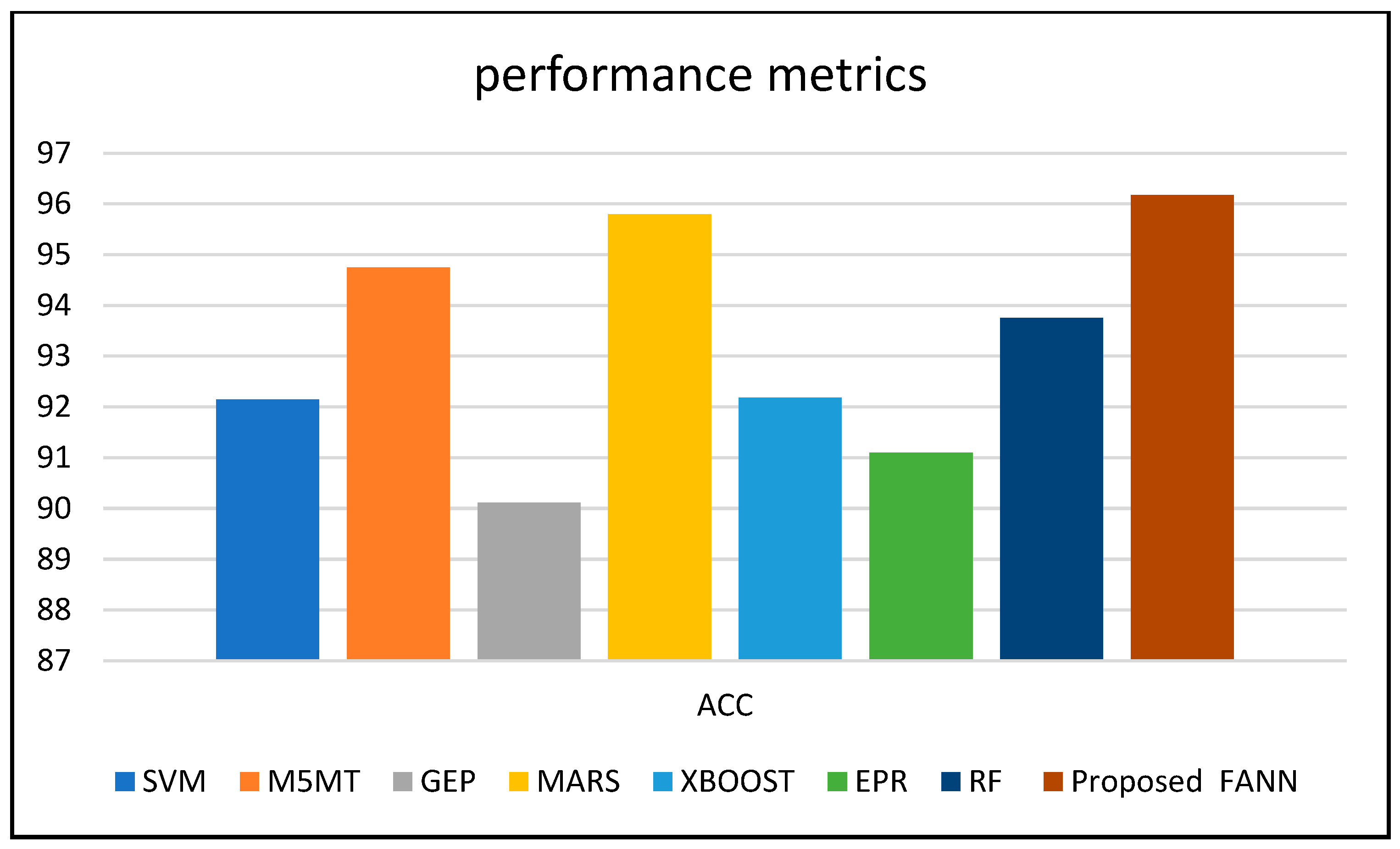
Figure 11 shows the comparison of the accuracy of the proposed work, with an SVM of 92.14%, M5MT of 94.75%, GEP of 90.12%, MARS of 95.79%, XBOOST of 92.18%, EPR of 91.1%, RF of 93.75%, and proposed FANN of 96.17%.
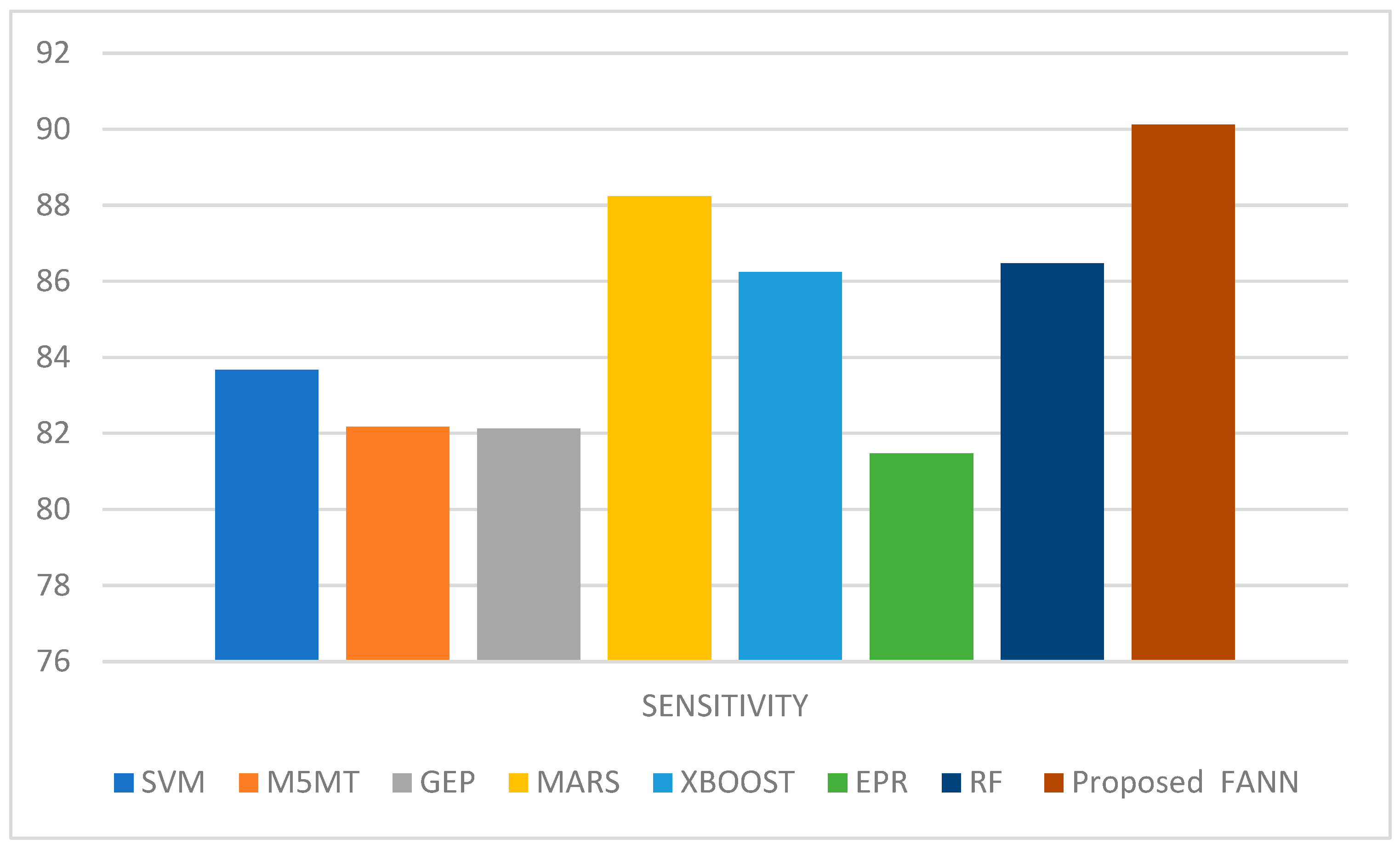
Figure 12 shows the sensitivity comparison of the proposed work, with an SVM of 83.67%, M5MT of 82.17%, GEP of 82.13%, MARS of 88.24%, XBOOST of 86.24%, EPR of 81.47%, RF of 93.75%, and proposed FANN of 96.17%.
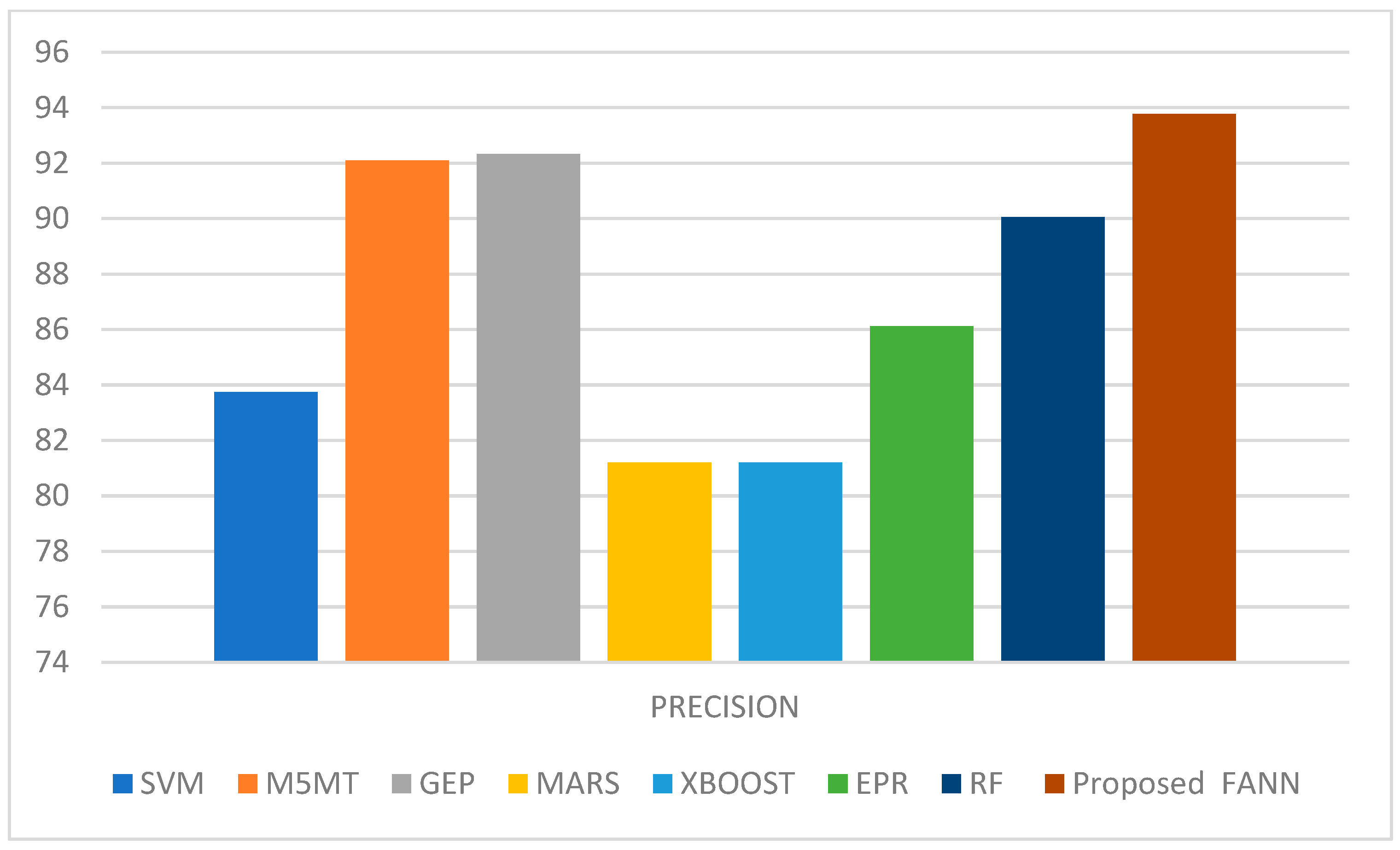
Figure 13 shows the precision comparison of the proposed work, with an SVM of 83.74%, M5MT of 92.1%, GEP of 92.33%, MARS of 81.2%, XBOOST of 81.2%, EPR of 86.12%, RF of 90.05%, and proposed FANN of 93.78%.
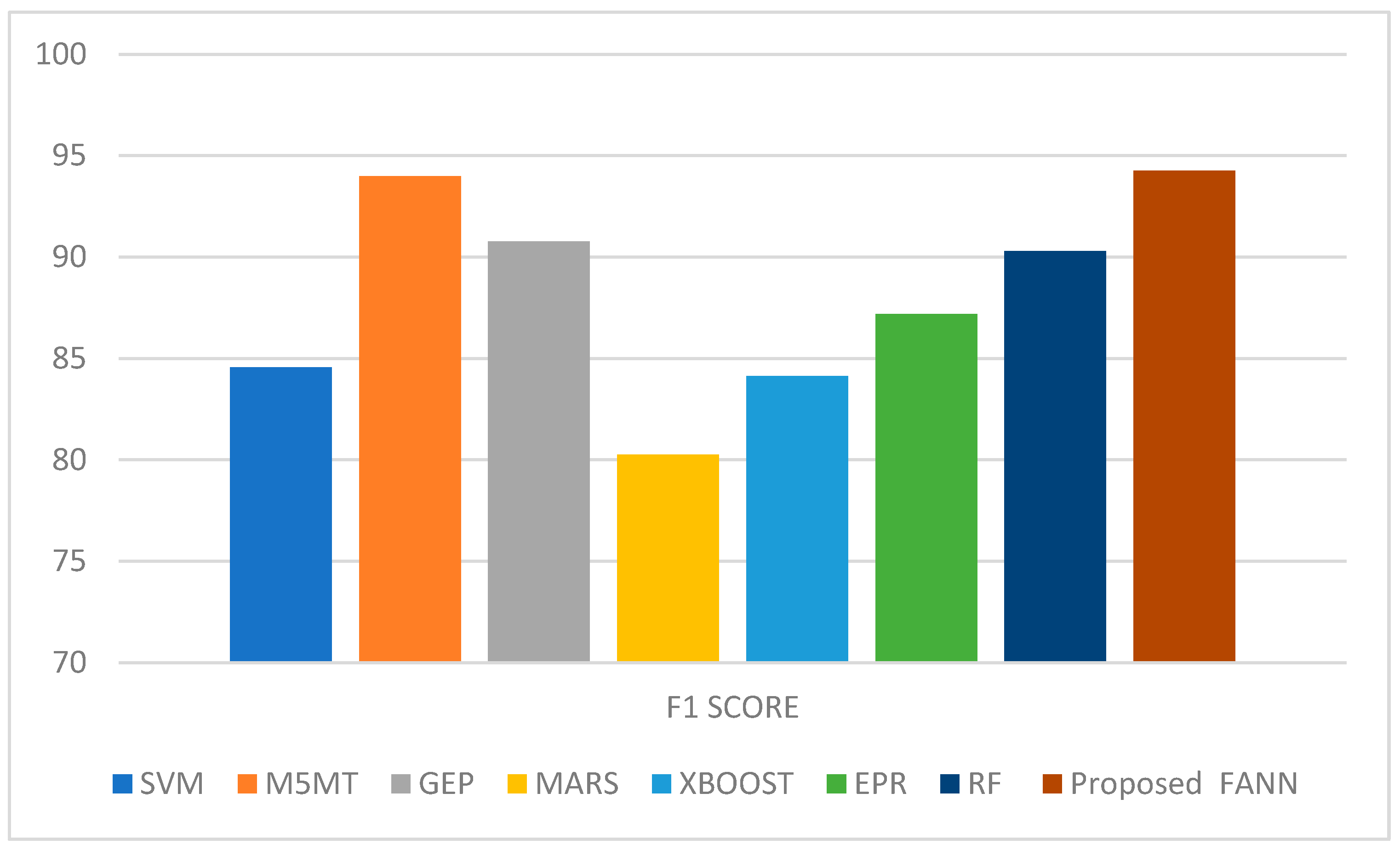
Figure 14 shows the F1 score comparison of the proposed work, with an SVM of 84.56%, M5MT of 93.99%, GEP of 90.78%, MARS of 80.26%, XBOOST of 84.13%, EPR of 87.19%, RF of 90.30%, and proposed FANN of 94.25%.
5. Conclusions
Working in RP is difficult because it requires constant attention to variables such as wind speed, humidity, temperature, pressure related to geo potential height, and atmospheric movement with rainfall. This endeavor consequently has the lowest chance of success. The proposed operation made heavy use of many classification algorithms, all of which are rooted in data mining. Various classification techniques exist, and the advantages of utilizing these approaches are evident in many applications. In addition, there is flexibility in how the rainfall information is recorded, with both monthly and daily recordings possible. As a result, it is crucial to select a tactic that works best for the amount of rain that has fallen. Since precipitation is the key component contributing to the formation of potential disasters such as tornadoes and hurricanes, accurate forecasting will assist in the process of preparing for a probable catastrophe. In this study, statistical measures were used alongside ML methods to forecast future behavior. Using a combination of data mining methods, we were able to estimate how much precipitation was needed to harvest the farm crops successfully. The major approaches used to calculate the rainfall model in Saudi Arabia include empirical and dynamical methods. The reliability of empirical progress is evaluated by examining historical data. The IMD database available on the government website was considered over the course of this study. Based on historical data, this database includes both extreme rainfall and more typical monthly and yearly rainfall totals. Farmers may utilize information about rainfall amounts to better plan their harvests. Data cleansing and classification are key parts of the developed machine learning system. Compared to other methods of classification, the results showed that the FFANN classifier performed very well. To classify data, the DT classifier achieved a success rate of 96.1%, which was 2.22 percentage points higher than the RF classifier, 4 percentage points higher than the ANN classifier, 4.99 percentage points higher than the SVM classifier, 7.3 percentage points higher than the KNN classifier, and 13.33 percentage points higher than the MLR classifier. Therefore, the proposed method is beneficial for forecasting the rainfall region at any time. To predict crop yields, LR is used, and for rice, maize, and gram, the R2 value is close to 0.9. Machine learning algorithms have CY models built in with drought variables, demonstrating the model’s utility in agricultural settings. When a user is located in an area with a high probability of experiencing adverse weather, the Global Positioning System (GPS) may be used to create location-based weather warnings for that area. It is possible that in the not-too-distant future, the online application will be modified to include information in regional and/or vernacular languages. Additionally, the implementation of email notifications may be a successful approach. For the benefit of customers who are visually handicapped, warnings may be customized as “voice notification alerts”.
Author Contributions
Conceptualization, M.B. and S.K.S.; methodology, M.B. and S.K.S.; validation M.B. and S.K.S.; formal analysis, M.B. and S.K.S.; investigation, M.B. and S.K.S.; resources, S.K.S.; data curation, M.B. and S.K.S.; writing—original draft preparation, S.K.S.; writing—review and editing, M.B. and S.K.S.; visualization, M.B. and S.K.S.; supervision, M.B. and S.K.S.; project administration, M.B. and S.K.S.; funding acquisition, M.B. All authors have read and agreed to the published version of the manuscript.
Funding
The authors extends their appreciation to the deputyship for Research & Innovation, Ministry of Education in Saudi Arabia for funding this research work through project number (IFP-2020-19).
Conflicts of Interest
The authors declare no conflict of interest.
Appendix A
| Algorithm A1 Pseudo code of Proposed forecasting model |
| and Threshold theta . Step 2 until condition is fake, execute steps Step 3 Execute step 5–7 for each training pair. Step 4 The input byer gets information and training it to concealed layer by executing identify activation function on the inputs form to 20. Step 5 Calculation of response of each response per unit as follow: to 15. Step 6 Calculate estimated output hidden_em habden_sf weights where weighted = effort multiplier weigh and weights m scale factor weight. Step 7 If weights still need to be updated. Go to step 10. Step 8 If the difference is within acceptable limit, the output is considered eke weights are modified using Firefly algorithm. Step 9 Repeat step 5 and step 6. Step 10 Calculate Magnitude of Relative Error, Step 11 Stop. |
References
- Parmar, A.; Mistree, K.; Sompura, M. Machine learning techniques for rainfall prediction: A review. In Proceedings of the International Conference on Innovations in information Embedded and Communication Systems, Coimbatore, India, 17–18 March 2017; Volume 3. [Google Scholar]
- Basha, C.Z.; Bhavana, N.; Bhavya, P.; Sowmya, V. Rainfall prediction using machine learning & deep learning techniques. In Proceedings of the 2020 International Conference on Electronics and Sustainable Communication Systems (ICESC), Coimbatore, India, 2–4 July 2020; pp. 92–97. [Google Scholar]
- Cramer, S.; Kampouridis, M.; Freitas, A.A.; Alexandridis, A.K. An extensive evaluation of seven machine learning methods for rainfall prediction in weather derivatives. Expert Syst. Appl. 2017, 85, 169–181. [Google Scholar] [CrossRef] [Green Version]
- Fahad, S.; Su, F.; Khan, S.U.; Naeem, M.R.; Wei, K. Implementing a novel deep learning technique for rainfall forecasting via climatic variables: An approach via hierarchical clustering analysis. Sci. Total Environ. 2023, 854, 158760. [Google Scholar] [CrossRef]
- Diez-Sierra, J.; Del Jesus, M. Long-term rainfall prediction using atmospheric synoptic patterns in semi-arid climates with statistical and machine learning methods. J. Hydrol. 2020, 586, 124789. [Google Scholar] [CrossRef]
- Refonaa, J.; Lakshmi, M.; Dhamodaran, S.; Teja, S.; Pradeep, T.N.M. Machine learning techniques for rainfall prediction using neural network. J. Comput. Theor. Nanosci. 2019, 16, 3319–3323. [Google Scholar] [CrossRef]
- Salman, A.G.; Kanigoro, B.; Heryadi, Y. Weather forecasting using deep learning techniques. In Proceedings of the 2015 international conference on advanced computer science and information systems (ICACSIS), Depok, Indonesia, 10–11 October 2015; pp. 281–285. [Google Scholar]
- Kapp, S.; Choi, J.K.; Hong, T. Predicting industrial building energy consumption with statistical and machine-learning models informed by physical system parameters. Renew. Sustain. Energy Rev. 2023, 172, 113045. [Google Scholar] [CrossRef]
- Barrera-Animas, A.Y.; Oyedele, L.O.; Bilal, M.; Akinosho, T.D.; Delgado, J.M.D.; Akanbi, L.A. Rainfall prediction: A comparative analysis of modern machine learning algorithms for time-series forecasting. Mach. Learn. Appl. 2022, 7, 100204. [Google Scholar] [CrossRef]
- Schultz, M.G.; Betancourt, C.; Gong, B.; Kleinert, F.; Langguth, M.; Leufen, L.H.; Mozaffari, A.; Stadtler, S. Can deep learning beat numerical weather prediction? Philos. Trans. R. Soc. A 2021, 379, 20200097. [Google Scholar] [CrossRef] [PubMed]
- Chkeir, S.; Anesiadou, A.; Mascitelli, A.; Biondi, R. Nowcasting extreme rain and extreme wind speed with machine learning techniques applied to different input datasets. Atmos. Res. 2023, 282, 106548. [Google Scholar] [CrossRef]
- Hong, W.C. Rainfall forecasting by technological machine learning models. Appl. Math. Comput. 2008, 200, 41–57. [Google Scholar] [CrossRef]
- Ridwan, W.M.; Sapitang, M.; Aziz, A.; Kushiar, K.F.; Ahmed, A.N.; El-Shafie, A. Rainfall forecasting model using machine learning methods: Case study Terengganu, Malaysia. Ain Shams Eng. J. 2021, 12, 1651–1663. [Google Scholar] [CrossRef]
- Fayaz, S.A.; Zaman, M.; Butt, M.A. Knowledge discovery in geographical sciences—A systematic survey of various machine learning algorithms for rainfall prediction. In International Conference on Innovative Computing and Communications; Springer: Singapore, 2022; pp. 593–608. [Google Scholar]
- Sumi, S.M.; Zaman, M.; Hirose, H. A rainfall forecasting method using machine learning models and its application to the Fukuoka city case. Int. J. Appl. Math. Comput. Sci. 2012, 22, 841–854. [Google Scholar] [CrossRef] [Green Version]
- Appiah-Badu, N.K.A.; Missah, Y.M.; Amekudzi, L.K.; Ussiph, N.; Frimpong, T.; Ahene, E. Rainfall Prediction Using Machine Learning Algorithms for the Various Ecological Zones of Ghana. IEEE Access 2021, 10, 5069–5082. [Google Scholar] [CrossRef]
- Khan, M.I.; Maity, R. Hybrid deep learning approach for multi-step-ahead daily rainfall prediction using GCM simulations. IEEE Access 2020, 8, 52774–52784. [Google Scholar] [CrossRef]
- Wong, K.W.; Wong, P.M.; Gedeon, T.D.; Fung, C.C. Rainfall prediction model using soft computing technique. Soft Comput. 2003, 7, 434–438. [Google Scholar] [CrossRef]
- Shah, U.; Garg, S.; Sisodiya, N.; Dube, N.; Sharma, S. Rainfall prediction: Accuracy enhancement using machine learning and forecasting techniques. In Proceedings of the 2018 Fifth International Conference on Parallel, Distributed and Grid Computing (PDGC), Solan, India, 20–22 December 2018; pp. 776–782. [Google Scholar]
- Dong, J.; Zeng, W.; Wu, L.; Huang, J.; Gaiser, T.; Srivastava, A.K. Enhancing short-term forecasting of daily precipitation using numerical weather prediction bias correcting with XGBoost in different regions of China. Eng. Appl. Artif. Intell. 2023, 117, 105579. [Google Scholar] [CrossRef]
- Raja, M.N.A.; Shukla, S.K. Predicting the settlement of geosynthetic-reinforced soil foundations using evolutionary artificial intelligence technique. Geotext. Geomembr. 2021, 49, 1280–1293. [Google Scholar] [CrossRef]
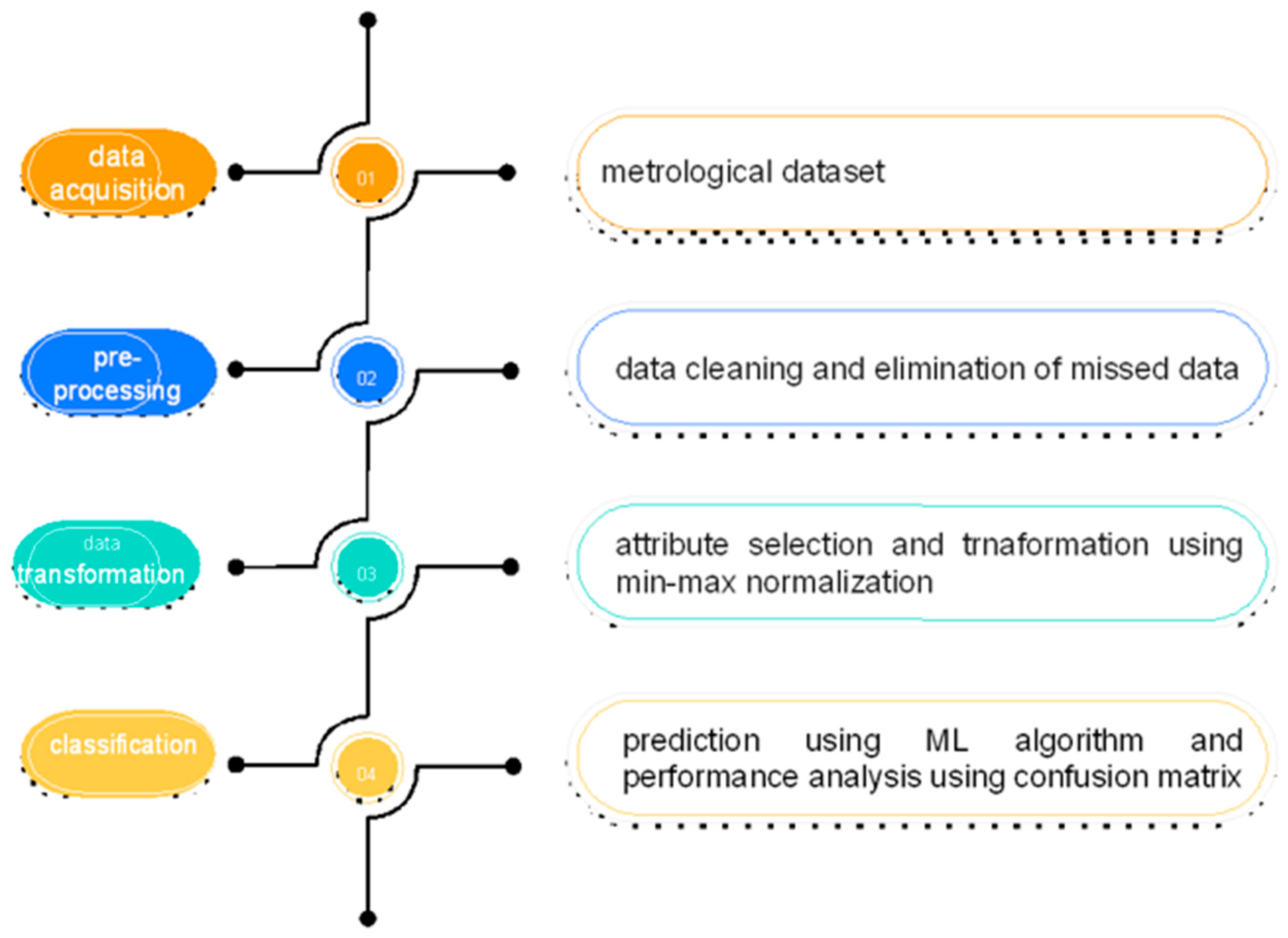
Figure 1.
Block diagram of the proposed work.

Figure 2.
Data tuning input model.

Figure 3.
Working of FFANN network.

Figure 4.
GUI window in prediction.

Figure 5.
Training epochs.

Figure 6.
Testing neural network.

Figure 7.
Training parameters.

Figure 8.
Validation rate.

Figure 9.
Crop yield prediction.

Figure 10.
Accuracy rate of crops.

Figure 11.
Accuracy comparison between proposed work and existing work.

Figure 12.
Sensitivity comparison between proposed work and existing work.

Figure 13.
Precision comparison between proposed work and existing work.

Figure 14.
F1 score comparison between proposed work and existing work.

Figure 15.
Specificity comparison between proposed work and existing work.


Table 1.
The attributes with the range variable and range values.
| Attributes | Range Variables | Range Values |
|---|---|---|
| Temperature | ||
| Dew Point | ||
| Visibility in Miles | ||
| Precipitation |
Table 2.
Predicted rate.
| Actual Rate (x) | Predicted Rate | Difference D = abs(x − y) | PE |
|---|---|---|---|
| 0 | 0 | ||
| 3479 | 3479 | 0 | 0 |
| 3576 | |||
| 0 | 0 | ||
| 0 | 0 | ||
| 3762 | 3762 | 0 | 0 |
Disclaimer/Publisher’s Note: The statements, opinions and data contained in all publications are solely those of the individual author(s) and contributor(s) and not of MDPI and/or the editor(s). MDPI and/or the editor(s) disclaim responsibility for any injury to people or property resulting from any ideas, methods, instructions or products referred to in the content. |
© 2023 by the authors. Licensee MDPI, Basel, Switzerland. This article is an open access article distributed under the terms and conditions of the Creative Commons Attribution (CC BY) license (https://creativecommons.org/licenses/by/4.0/).
Share and Cite
MDPI and ACS Style
Baljon, M.; Sharma, S.K. Rainfall Prediction Rate in Saudi Arabia Using Improved Machine Learning Techniques. Water 2023, 15, 826. https://doi.org/10.3390/w15040826
AMA Style
Baljon M, Sharma SK. Rainfall Prediction Rate in Saudi Arabia Using Improved Machine Learning Techniques. Water. 2023; 15(4):826. https://doi.org/10.3390/w15040826
Chicago/Turabian StyleBaljon, Mohammed, and Sunil Kumar Sharma. 2023. "Rainfall Prediction Rate in Saudi Arabia Using Improved Machine Learning Techniques" Water 15, no. 4: 826. https://doi.org/10.3390/w15040826
Note that from the first issue of 2016, this journal uses article numbers instead of page numbers. See further details here.