Abnormal Waves Observation and Analysis of the Mechanism in the Pearl River Estuary, South China

Abstract

The Pearl River Estuary is a typical estuary region in southern China, and the study of surface wave occurrence and characteristics is of great importance for shipping management, nearshore engineering, and monitoring shoreline changes and other human activities. Long-term and continuous observational data are critical for achieving a better understanding of waves. In this study, the wave measurements based on a high-precision wave gauge were analyzed and observation data over approximately two years at a sampling frequency of 2 Hz were obtained. The wave system in the Pearl River Estuary was found to deviate from the assumption of a stationary stochastic process similar to that in the open ocean, due to the effects of abnormal waves caused by human activities. Therefore, traditional distribution functions such as Rayleigh and Weibull were not suitable for accurately fitting the main wave parameters ($H_s$, $T_p$, etc.), particularly in the tail. Consequently, abnormal wave signals were extracted from all wave sets, and through the comparison and analysis of the wave spectral features, it was determined that these abnormal waves are caused by the ship wakes. The spectral characterization of these waves was performed to determine the characteristics of different ship wake processes. Ship wakes in the Pearl River Estuary are an important part of the wave system, and their wave height is significantly larger than the normal wave. Based on the spectral characteristics of ship wakes, this study proposed some news characteristics of ship wakes in the main channel of the Pearl River Estuary.

1. Introduction

The Pearl River Estuary (PRE) is located on the southern coast of China, adjacent to the continental shelf of the northern South China Sea. The PRE sustains large populations and productive ecosystems regionally. Marine environment dynamic systems, including waves, are critical for the sustainable development of socio-economic activities and ecosystems [1,2,3,4,5,6,7]. The PRE is a bell-shaped estuary [8] with a complex estuarine bathymetry [9,10,11]; thus, it is a complex dynamic system. As waves influence shipping, harbor operations, nearshore engineering construction, and sediment resuspension, wave observation in estuaries is critical.

Recently, remote sensing data and ocean numerical model data have been widely used to study regional wave systems [12,13,14,15,16]. With a moderate spatial resolution, WaveWatch3 and ECMWF are the most commonly used ocean numerical model datasets of wave data [12,17,18]. For the medium/small-scale wave models, nonlinear Boussinesq models were widely used [19,20,21]. These models and data have wide applicability and are suitable for large-scale applications; however, they cannot replace in situ observations with high-precision and high-frequency sampling. Wave observations are particularly useful for the study of small-scale water surface abnormal fluctuations (e.g., ship wakes, freak wave, sea level monitoring, and air–sea interaction).

To better understand the wave climate of a target area, studies are conducted in the area to calculate and analyze the spatiotemporal distribution of the wave height and wave period [15,22,23,24,25]. In oceans, waves are generated by strong and frequent winds over long fetch lengths; these waves propagate to the coast with large amplitudes. Wave heights can exceed 10 m or dozens of meters. In most estuaries, winds are infrequent, and wind speeds are relatively low. In addition, wind forcing at the water surface generally varies at small spatial scales, and the effective fetch length is restricted to several kilometers. Hence, the wave field in most estuaries is characterized by waves with small amplitudes and high frequencies; therefore, this wave field differs considerably from the wave field in the ocean [26]. However, besides wind waves, surface waves generated by large freighters and tourist ship traffic are important components of wave systems in estuarine, lagoon, and lake areas with high human activity. Moreover, they are currently the focus of extensive research in this field [27,28,29,30,31,32]. In Lake Constance, in particular, ship-generated waves are as important as wind-generated waves and they contribute approximately 41% of the annual mean wave energy flux to the shore [26]. In contrast to wind waves that occur only sporadically, ship waves propagate into the littoral zone frequently at regular time intervals. The different patterns of the occurrence of ship and wind waves result in different patterns of disturbance in the littoral ecosystem. These ship wakes propagate as long-term, strongly nonlinear, solitary Riemann waves of depression over substantial distances into the Venice Lagoon. Unexpectedly high (up to 2.5 m) solitary depression waves are generated by moderately sized ships sailing at moderate-depth Froude numbers and block coefficients in channels surrounded by shallow banks. These ship waves can propagate to a distance of up to 500 m from the navigation channel [33,34]. In the above-mentioned studies, theoretical analysis and observations under specific environmental conditions (such as ships or short-term observations) were the main research methods and fundamental data. However, there have been few reports on the analysis of the causes and inherent structure of abnormal waves from large amounts of high-frequency continuous data.

To better understand the internal structure of the wave systems in the PRE, we developed a high-precision and high-sampling-frequency wave meter with a pressure sensor over more than two years. In the data, lots of abnormally large wave heights were observed. By utilizing these high-frequency continuous data and combining frequency domain analysis methods, the inherent structure of abnormal waves in the Pearl River Estuary is revealed, and the causes of the abnormal waves are identified.

In this study, a dataset was created by collecting the data recorded by a wave meter, SZS3-1, for more than 2 years at a sampling frequency of 2 Hz. The principle of the instrument used and the parameters used for measurement are described in Section 2. The statistics and distribution of the wave parameters are presented and discussed in Section 3.1. The characterization of the ship wake based on the wave spectra is described in Section 3.2. The main findings of the study are summarized in Section 4, which concludes the paper.

2. Instrument and Methods

2.1. Principle of the Instrument

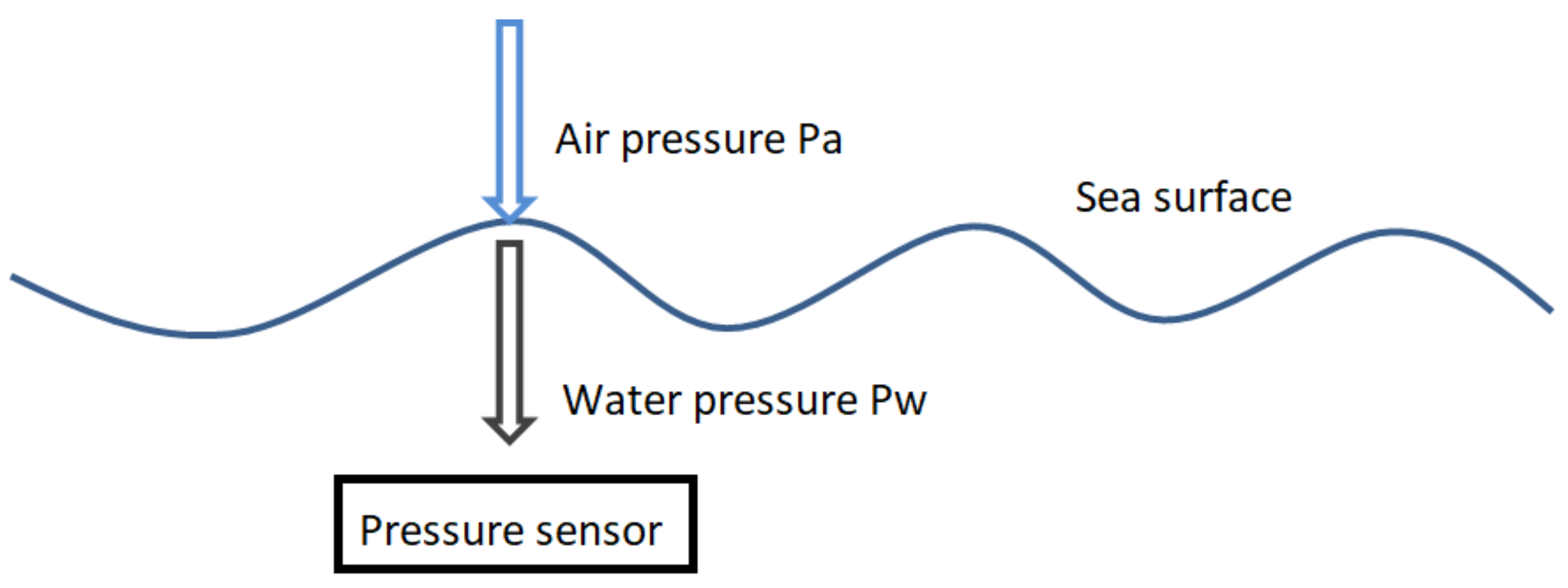
As illustrated in Figure 1, the wave gauge was mounted on a stationary platform below the water surface, and air pressure was introduced into the pressure sensor via the water body transmission. Thus, the pressure measured was the sum of the atmospheric and seawater pressures. Using $P=P_a+P_w=P_a+\rho gh$ and $H=\left(P-P_a/\rho g\right)$, the measured pressure signals can be converted into water surface height signals. In the above equations, P is the total pressure measured by the pressure sensor (average value after filtering out the wave pressure variations), $P_a$ is the atmospheric pressure, $P_w$ is the water pressure, $\rho$ is the average density of seawater from the sensor to the sea surface, $g$ is the gravity at the measuring site, and $H$ is the vertical height from the pressure sensor to the water surface.

We assumed that during the observation time, the change in the average density of seawater was insignificant, and the acceleration due to gravity, g, was constant at the selected release point in the conversion process of the water surface height signal. The total pressure measured by the pressure sensor and the atmospheric pressure measured by the barometer on the shore can be used to calculate the sea level, thereby obtaining the tide level. The various elements of the surface waves can be obtained by converting the pressure spectrum to the surface wave spectrum as follows:

$$S_0\left(w\right)=N^2{S}_p\left(\omega \right)\frac{c{h}^{2}kd}{c{h}^{2}k\left(d+z\right)},$$

(1)

$${\omega }^2=gk th\left(kd\right),$$

(2)

where $k$ is the wave number ($k=2\pi /L$, $L$ is the wavelength), $d$ is the water depth, $z$ is the pressure sensor depth, $S_0\left(\omega \right)$ is the surface wave spectrum, $S_p\left(\omega \right)$ is the pressure spectrum, $g$ is the acceleration due to gravity, $\omega$ is the wave circle frequency, and $N$ is the conversion coefficient. The corresponding wave height, period, and other wave elements can then be calculated using the surface wave spectrum.

2.2. Wave Instrument Composition

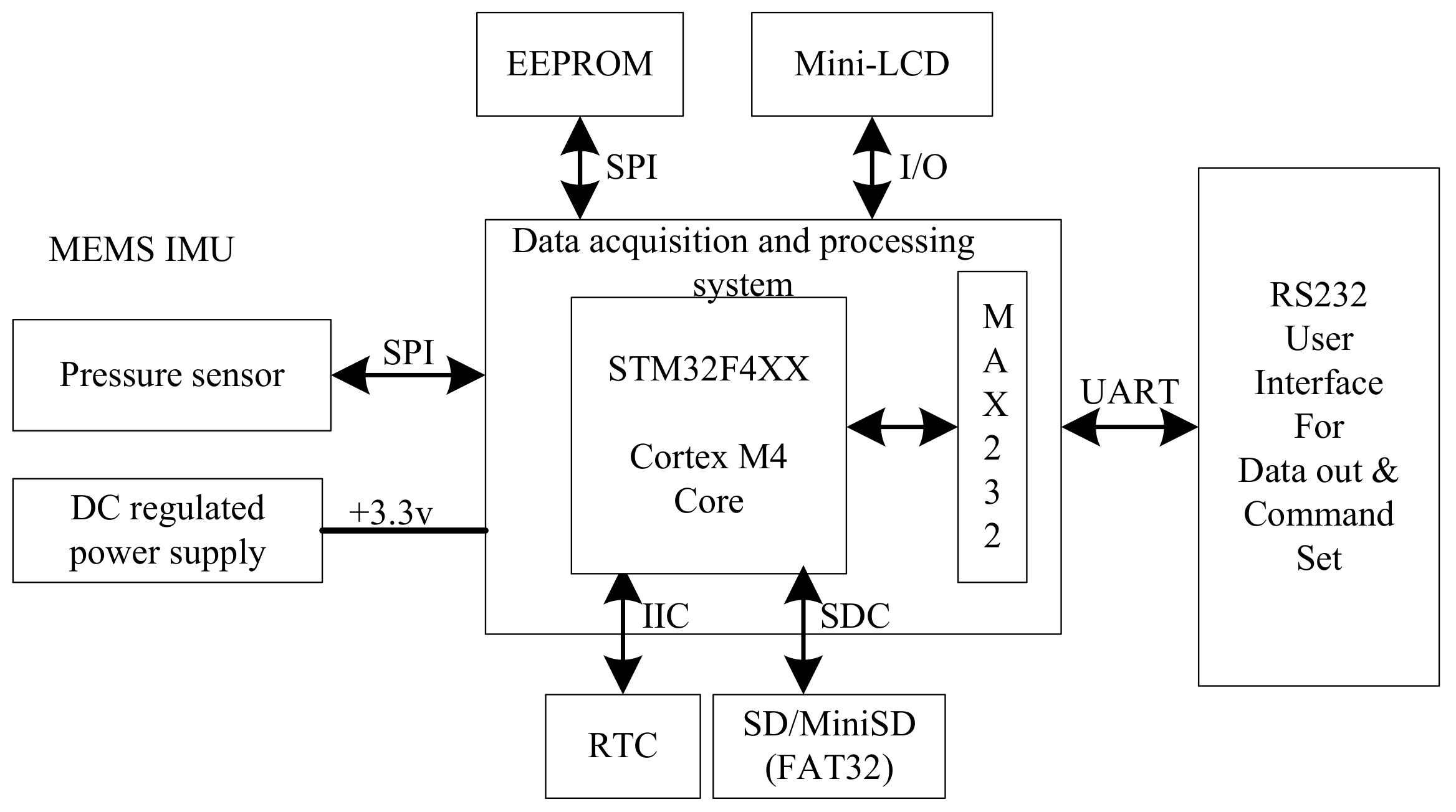
The wave meter (SZS3-1) included a high-precision pressure sensor, microcontroller, and memory. The design utilizes the microcontroller software resources and maximally replaces the hardware circuits with software methods, thus resulting in a simple, low-power, and high-reliability instrument circuit. The self-contained working time is long, and the system has real-time data processing capability. Automatic wave encryption observation is conducted according to the preset wave height threshold. In this study, the wave instrument was connected to a computer via an RS232 interface, and it was equipped with data reading, configuration, and communication software. This simplified the human–machine communication and operation, and the data output format could be directly adjusted to meet the needs. Through the cable socket on the end cover, we performed direct parameter setting and data playback on the instrument. Given that the instrument had a power-down memory function, the parameters did not require re-setting upon changing the battery, and the stored data were not lost. The instrument was equipped with an external switch and a working-status viewing window (Figure 2). The working status of the instrument can be understood using light-emitting diodes in the viewing window.

The pressure gauge signals were low-pass filtered to long-period of tidal fluctuations and converted to the elevation of surface waves following the conversion procedure provided by the instrument instruction. In the range of 0–8 m, the maximum indication error is 0.6 cm [35].

2.3. Data and Wave Parameters

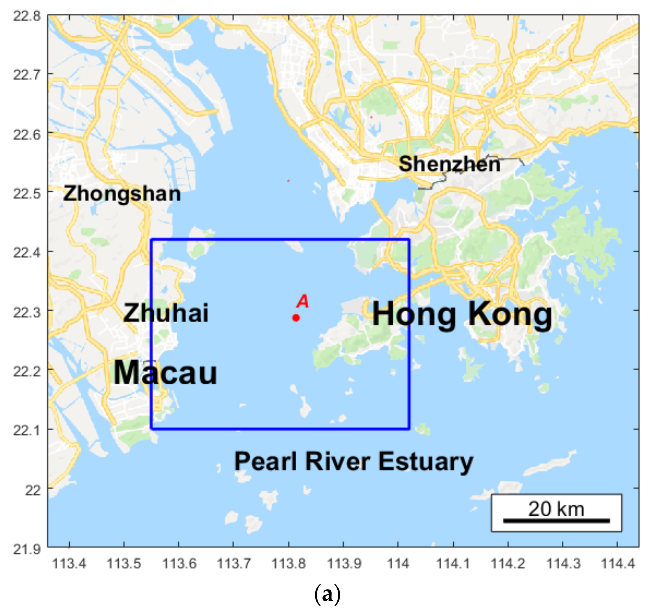
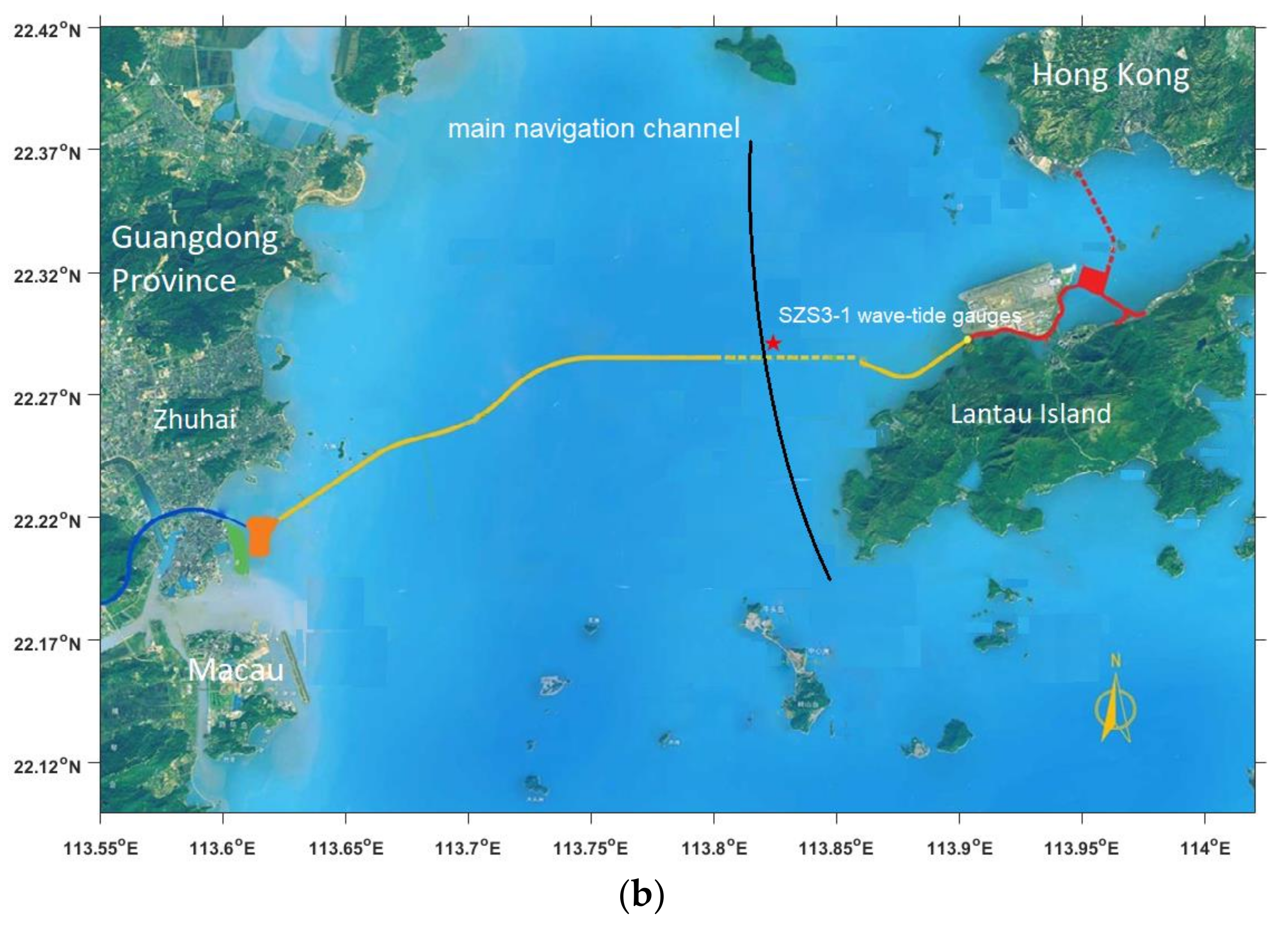
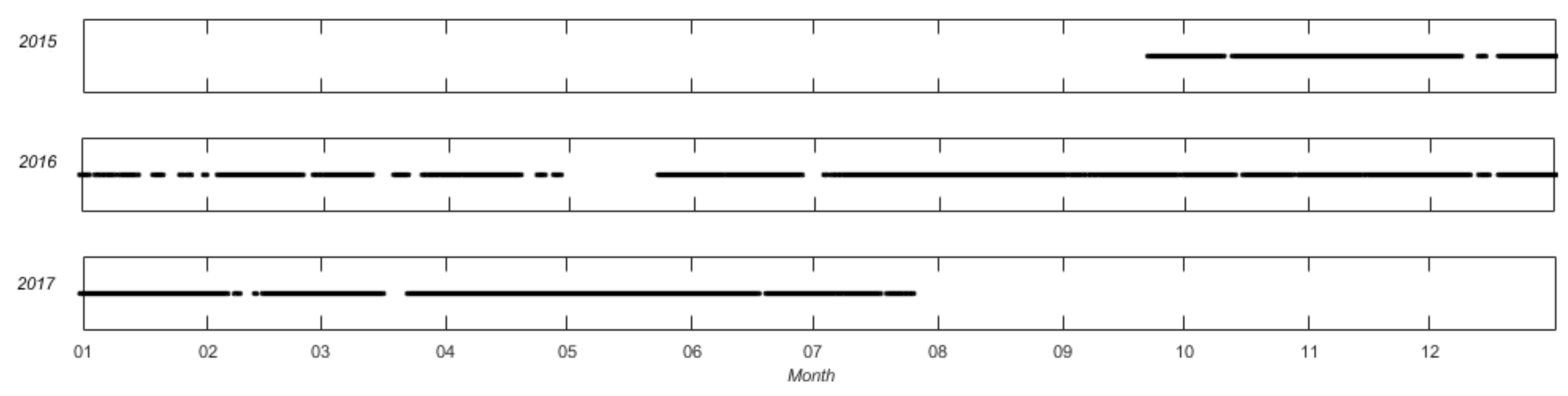
SZS3-1 wave-tide gauges were installed near the main channel of the PRE (Figure 3). with continuously operating pressure sensors at a sampling frequency of 2 Hz. The exact location was 22°17′15″ N, 113°48′49″ E, where the water depth was approximately 8 m, and the wave-tide gauges were installed 2 m below the water surface (observed mean water level) and fixed on a small ocean platform. The instrument recorded continuous data from 22 September 2015 to 15 July 2017 at a data completion rate of 89.1% (Figure 4).

The acquisition of wave characteristic parameters should satisfy the following principles:

(1) The original sample passes the 10 min sample segment sliding test to remove outliers with values greater than the mean + 3 × std (mean: mean, std: standard deviation).

(2) The number of samples is greater than 2400 × 2/3 = 1600; otherwise, the set of samples is removed.

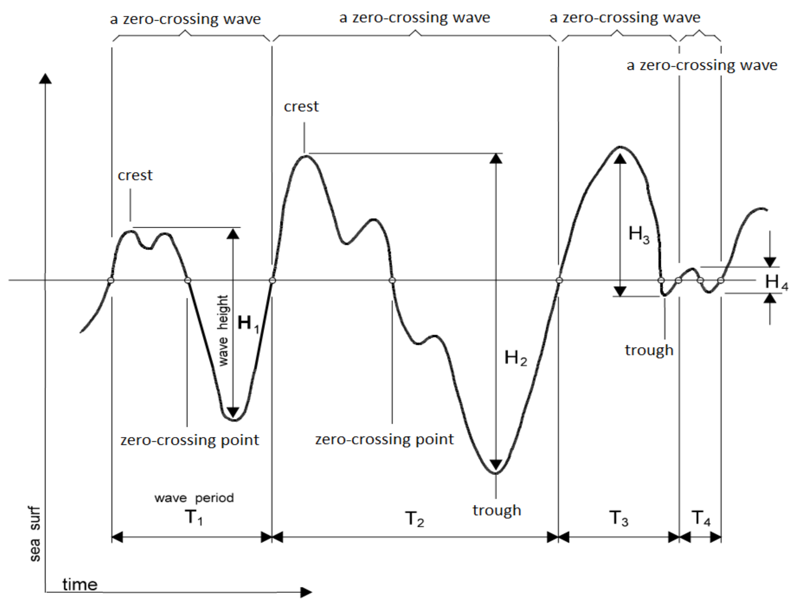
After the pressure data were converted into wave surface data, the main wave parameters (e.g., $H_s$, $T_p$, and $H_{m0}$) of each wave were determined using the zero-crossing statistical method and by calculating the wave spectrum. For the zero-crossing statistical method, a “wave” is defined as the portion of a record between two successive zero up-crossings (Figure 5). Therefore, the separation of wave crests and wave troughs is a prerequisite for the zero-crossing method. In this study, the time series of the crests and troughs of the wave trains were extracted using the WAFO software package [36]. Moreover, we set 1200 s as the statistical time window. If valid data are observed at all times during this window, a total of 2400 wave surface data in each window can be obtained with a sampling frequency of 2 Hz. The significant wave height ($H_s$ or $H_{1/3}$) is the mean of the highest one-third wave height and is calculated as follows:

$$H_s=\frac{1}{N/3}{\displaystyle \sum }_{i=1}^{N/3}{H}_i,$$

(3)

where $H_i$ is the highest one-third wave height, and $N$ is the number of zero-crossing waves. Similarly, the significant wave period ($T_{1/3}$) is the mean of the periods of the highest one-third waves and is calculated as follows:

$$T_{1/3}=\frac{1}{N/3}{\displaystyle \sum }_{i=1}^{N/3}{T}_i,$$

(4)

where $T_i$ is the highest one-third wave height, and $N$ is the number of zero-crossing waves.

From the calculated wave spectrum, the main wave parameters commonly used to describe the wave period and wave height can be obtained using the spectral moments.

$$H_{m0}=4\ast \sqrt{m_0},$$

(5)

$$T_p=\frac{1}{f_p}=\frac{1}{f\left(S_{MAX}\right)},$$

(6)

$$T_{m01}=\frac{m_0}{m_1},$$

(7)

$$\mathrm{Ss}=2\ast \mathrm{pi}\ast \mathrm{Hs}/\left(\mathrm{g}\ast T_{m02}{}^2\right),$$

(8)

where $H_{m0}$ is the significant wave height from the wave spectrum, $T_p$ and $T_{m01}$ are the peak and mean periods, respectively, and $\mathrm{Ss}$ is the significant wave steepness. The spectral moments are defined as follows:

$$m_n={{\displaystyle \int }}_0^{\infty }{f}^{n}S\left(f\right)df,$$

(9)

where $S\left(f\right)$ is the spectrum of the surface elevation.

According to conventional understanding, abnormal waves typically refer to a wave train that features extreme wave heights. Following the definition of rogue waves, abnormal waves were defining a wave train with individual waves exceeding 2.2 times the significant wave height. That is to say that $H_x\ge 2.2H_s$, where $H_x$ is the actual crest-to-trough (wave) height [2,37].

3. Results

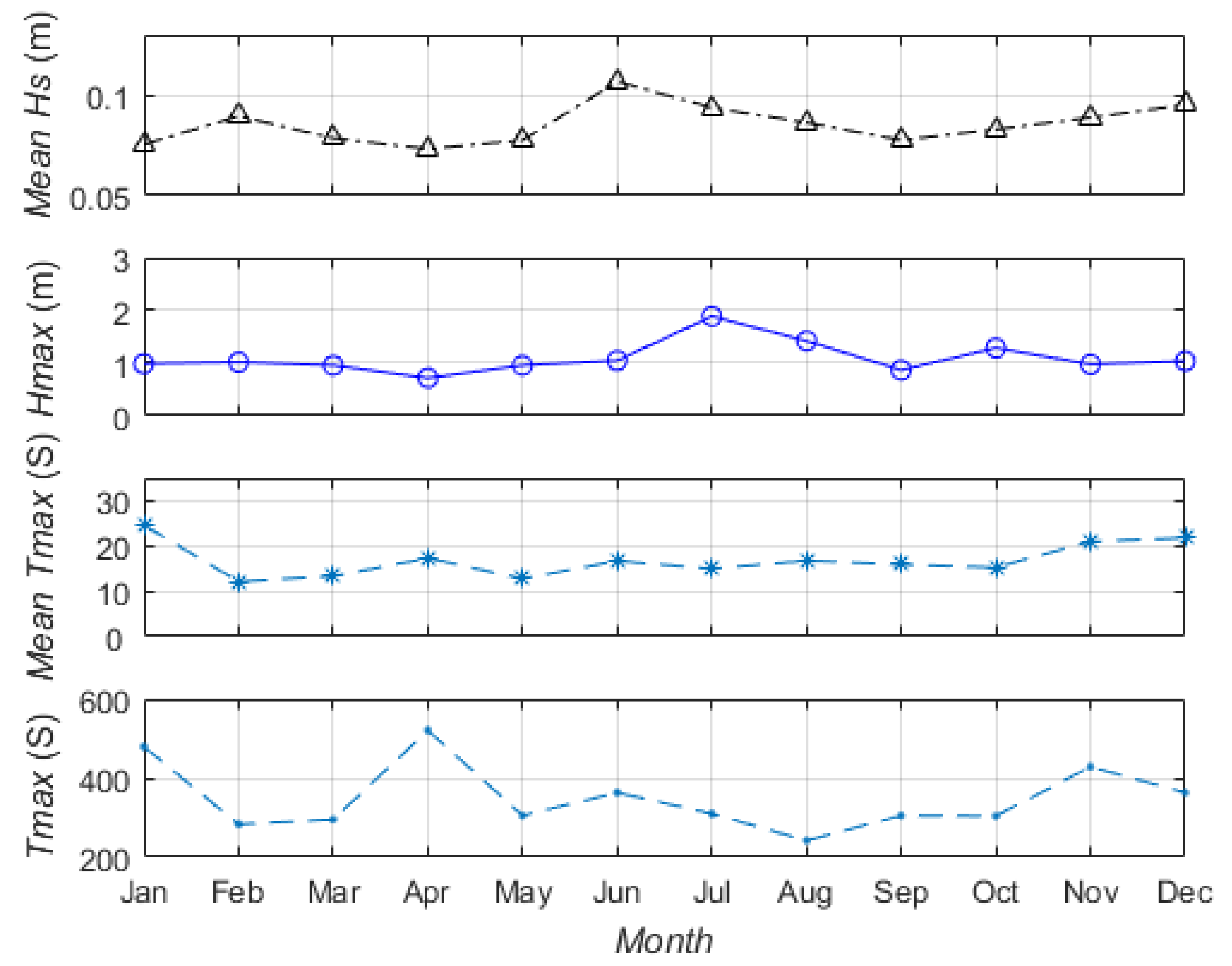
By using 1200 s as the time window to segment the original sample, a total of $n=\mathrm{37,145}$ wave parameters were obtained. As can be seen from Figure 6, the mean of $H_s$ over all the data is 0.0854 m, and the maximum wave height is 1.89 m. The maximum $T_{max}$ of 520.31 s was in April. Overall, the observed wave heights were small because the observation position (Figure 3) was located in the estuary and the area had many small islands that block the waves, especially swells, from the open sea. However, the maximum wave height and period were unexpectedly large.

This section details the analysis of the properties of all the wave sets to determine the actual characteristics of the waves in the PRE. The ship wakes were analyzed separately. By analyzing the characteristics of the observed waves, the validity of the sensor was verified, and the wave characteristics of the PRE, a shallow water estuary, were determined.

3.1. Wind Wave Parameters Statistics

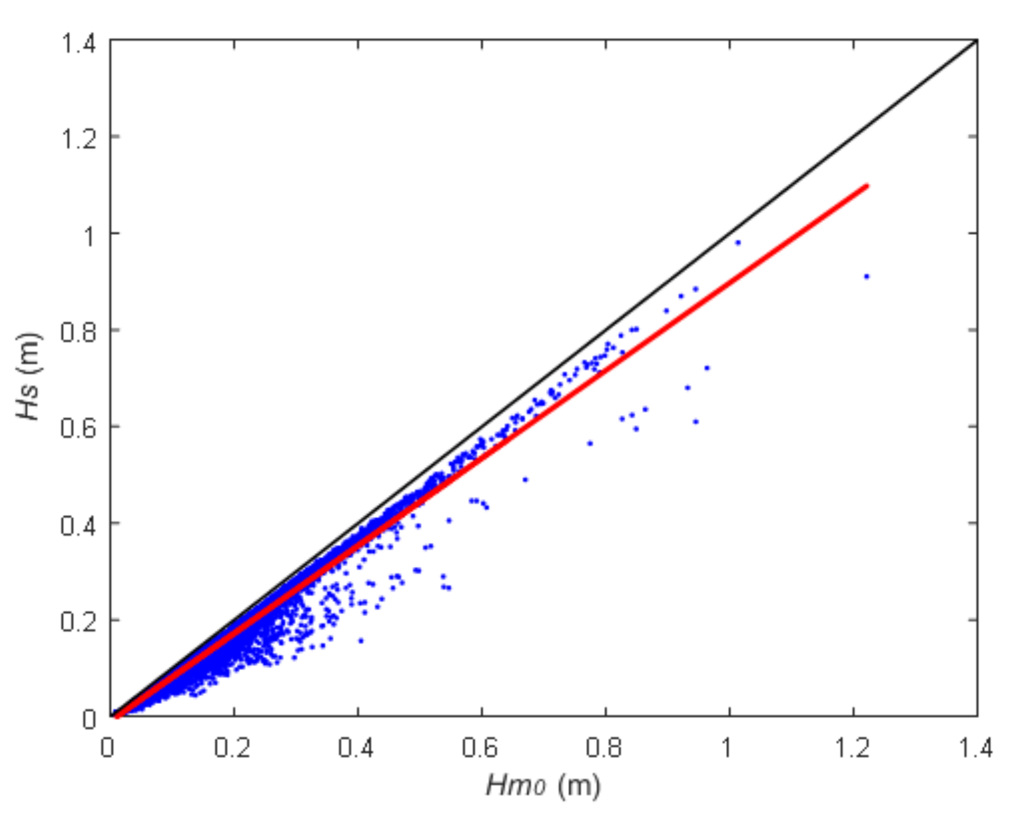
The significant wave heights, $H_s$ and $H_{m0}$, were obtained using the zero-crossing statistical method and calculating the wave spectrum. According to previous research, $H_s$ should be approximately equal to $H_{m0}$, and the correlation coefficient can reach 0.99. However, Figure 7 indicates that the correlation between $H_s$ and $H_{m0}$ was not excessively high. In particular, the correlation coefficient was only 0.9065, and $H_{m0}$ was slightly larger than $H_s$. This may be because the observed wave heights were too excessively small (the minimum value was in the millimeter scale) to be limited by the minimum precision of the instrument, and did not reflect the actual ocean wave process. Moreover, owing to several small disturbances caused by undetectable human activities, the fluctuation process may not satisfy the assumption of a stationary random process.

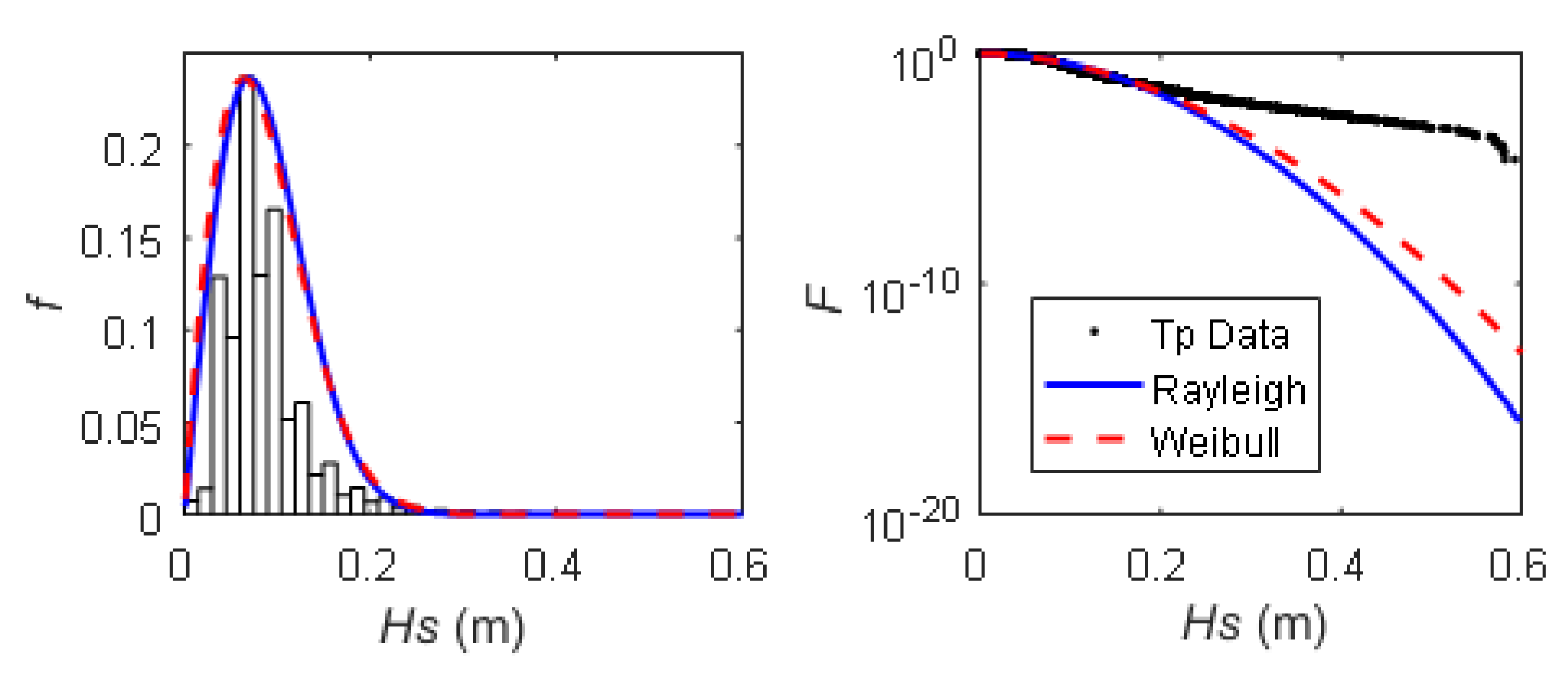
A statistical analysis of the main wave parameters was conducted using the parameters of the up-crossing significant wave height $H_s$. The analyses of $T_p$ and $T_{m01}$ revealed similar statistics. This paper only presents the results for $T_p$, as it is more commonly used to characterize the sea state. The probability distribution functions (PDFs) of the significant wave height and peak period are shown in Figure 8 and Figure 9, respectively. In previous studies, attempts were made to model the distributions of the wave height and period [23,24,38]. The description of the tail is particularly important for the engineering design. Several studies were conducted to describe and model the $H_s$ and $T_p$ distributions (e.g., [15,22,25].

The distribution of the wave height has been commonly associated with the theoretical Rayleigh or Weibull distributions, with the probability density functions of a variable $\epsilon$ expressed as follows:

$$p\left(\epsilon \right)=\frac{\epsilon }{a^2}{e}^{\frac{-{\epsilon }^2}{2a^2}},$$

(10)

$$p\left(\epsilon \right)=\frac{b}{a}{\left(\frac{\epsilon }{a}\right)}^{b-1}{e}^{\left[-{\left(\frac{\epsilon }{a}\right)}^2\right]},$$

(11)

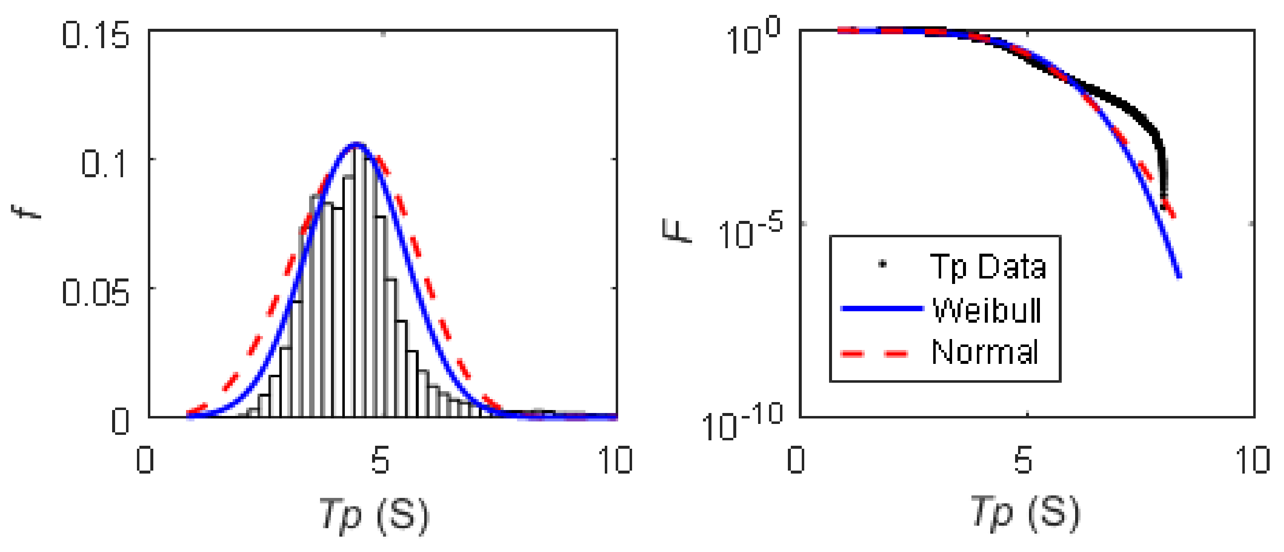
where $a$ and $b$ are the scale and shape parameters, respectively. A normal-type distribution is applied to characterize the wave period as follows:

$$p\left(\epsilon \right)=\frac{1}{\sigma \sqrt{2\pi }} e^{-\frac{{\left(\epsilon -\mu \right)}^2}{2a^2}},$$

(12)

where $\mu$ and $\sigma$ are the mean and standard deviation, respectively.

The Weibull and Rayleigh curves were plotted in comparison with $H_s$, as shown in Figure 8; the figure also shows the PDF and exceedance probability. From the observation location to areas inside the estuary, the waves were mainly wind waves, and the wave amplitudes were small. From the left panel, it can be seen that most of the $H_s$ values are less than 0.2 m. The Rayleigh and Weibull fits are in good agreement with the distribution for H_s < 0.1. However, neither model represented the upper tail. It should be noted that the $H_s$ values in the PRE do not accurately reflect the characteristics of wind waves.

Figure 9 presents the normalized distribution and Weibull distribution for $T_p$ corresponding to the full dataset. Similarly to $H_s$, the normal and Weibull fits were in good agreement with the peak period distribution obtained from the entire dataset. However, the tail was not accurately represented. The proportion of waves with larger periods increased significantly, as can be seen from the right panels of Figure 9, which may be due to ship wakes or other human influences.

3.2. Ship Wakes

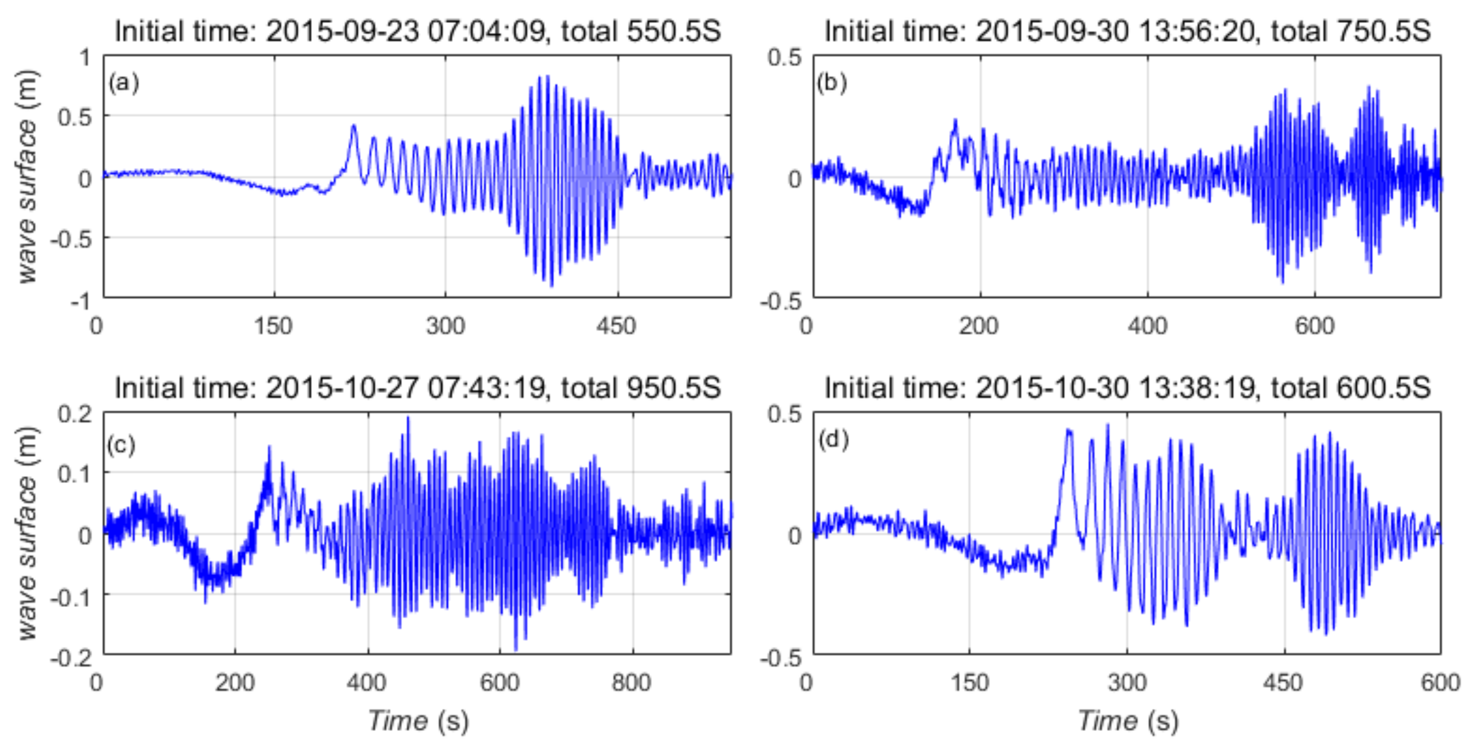
In addition to the analysis of all the waves in the previous section, the ship wake characteristics are discussed in this section. The four cases of ship wakes are shown in Figure 10. The sea level dropped unexpectedly (the depression referred to by [33] before the occurrence of the main wave of the ship wakes. The various features of the ship wakes are shown in Figure 10. As shown in Figure 10a, the frequency and amplitude increased abruptly after a period of relatively low frequency and small amplitude fluctuations. There were two consecutive abnormal fluctuations in the water surface, as shown in Figure 10b,d. Figure 10c presents a more unexpected case, in which relatively large amplitude fluctuations occurred for a longer period.

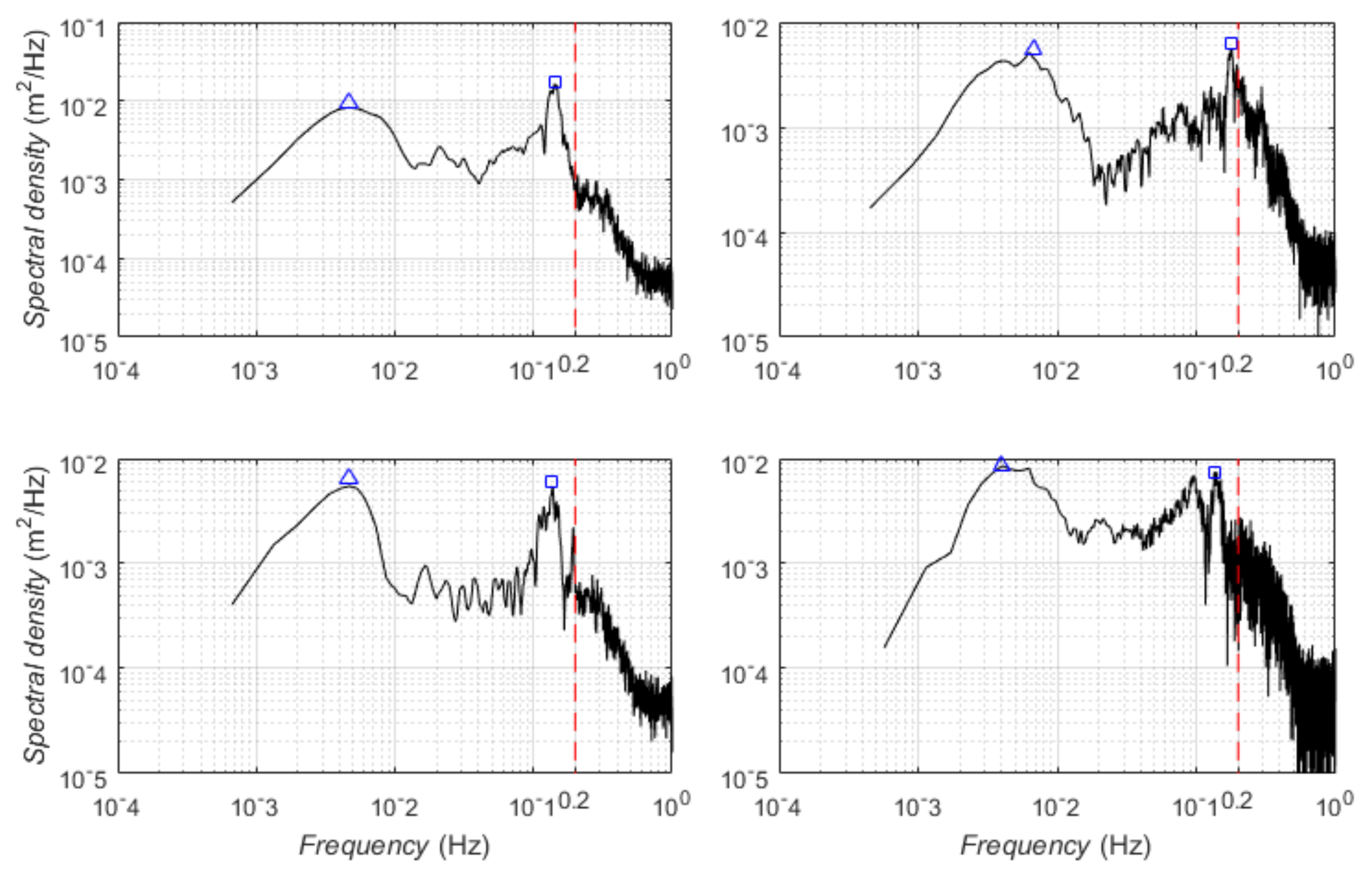
The occurrence of ship wakes was accompanied by an abrupt increase in the wave height, in addition to certain changes in the corresponding wave period. Therefore, we attempted to conduct a frequency domain analysis based on Fourier transform.

In the wave spectra, different peak frequencies or frequency bands can represent different ship-generated waves [26]. In the PRE, the four typical ship wake data were transformed into the frequency domain for the frequency analysis, as shown in Figure 11. The two peaks were clear in all the spectra. Both peaks correspond to two typical processes of the ship wakes: depression and main wave. In the frequency range $\left[{10}^{-3},{10}^{-2}\right]$ ($T\in \left[100, 1000\right]$), the peak can be attributed to the depression process, whereas in the frequency range [10⁻¹, 0.2] ($T\in \left[5, 10\right]$), the peak can be attributed to the main wave process. Thus, the characteristic spectral properties of wind and ship waves were used to discriminate between them at the threshold frequency of 0.2 Hz (T = 5 s). Waves with frequency peaks of below 0.4 Hz for the main wave and below ${10}^{-2}$ Hz for the depression can be attributed largely to the ship wake process rather than the wind wave process.

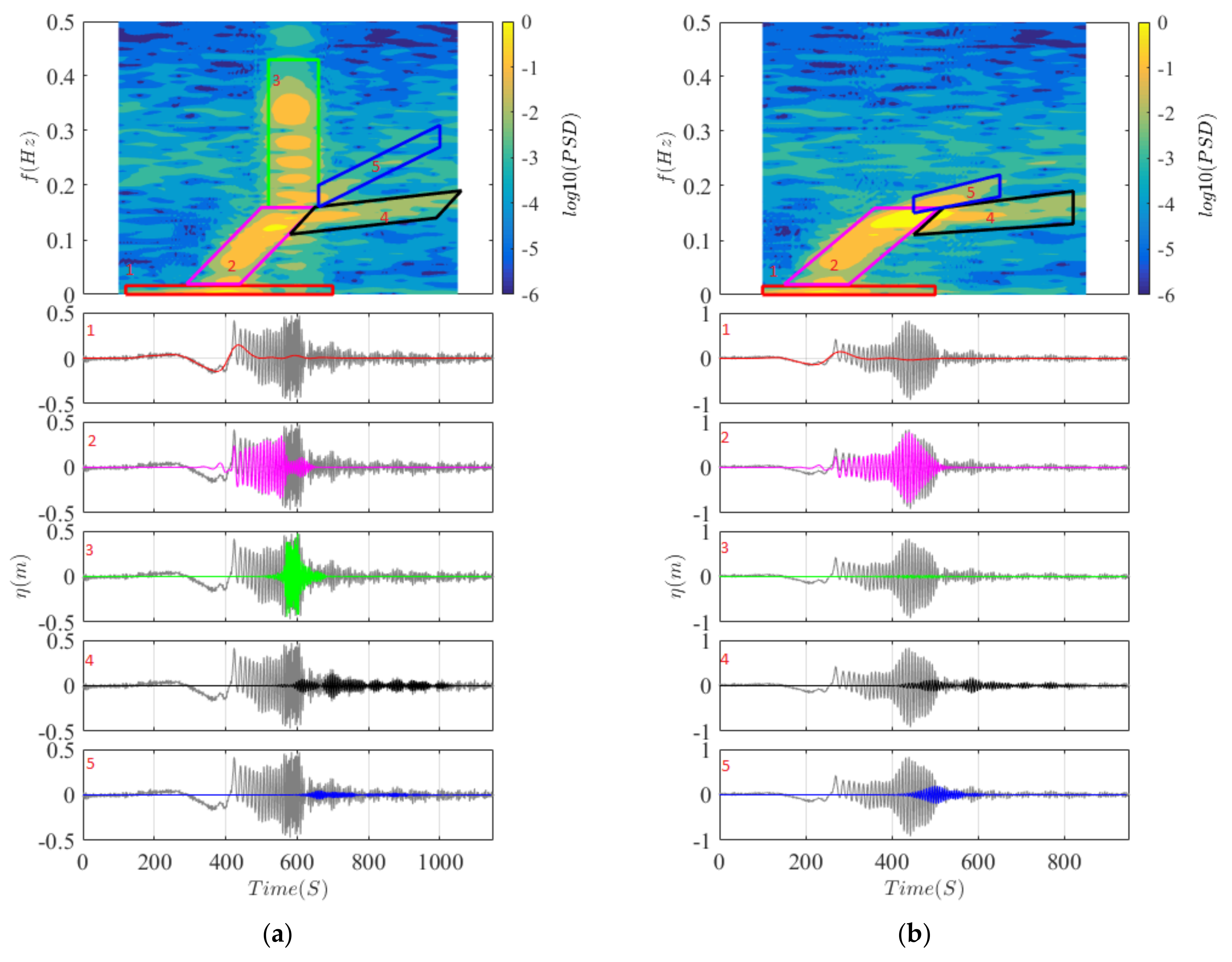
Another identification method of the ship wakes is based on the wave spectrogram. According to the cause of generation and the amount of energy carried, ship wakes can be divided into multiple parts. Torsvik et al. [39] divided the observed ship wakes in shallow water area into five parts: one, PW: precursor; two, LW: leading wave; three, TW: transverse wave, four, DW: divergent wave, and five, LF: low frequency. Additionally, it was proposed that these five features can be used as the basis for identifying ship wakes. Figure 12 shows two observed spectrograms of ship wakes, which have signals of TW and DW, which are most obvious as ship wakes. However, there are also some differences from the ship wakes in [39]. First, there is an obvious process of water level drop during the ship wake, which causes the two parts, PW and LF, to merge and leads to the energy of the low-frequency process being much larger than the PW and LF in [39]. This process is similar to that of ship-generated tsunamis [40,41,42,43], and will not be discussed here. Second, compared with Torsvik et al. [39], there is an additional transition process of primary wake chirp between the PW and LW. Third, the proportion of energy carried by DW and TW is smaller than that in [39]. In addition, in all the abnormal fluctuation observation data, not every ship traveling wave process has the above five characteristics, and the process shown in Figure 12b has no obvious LW process.

Since the observations did not record the information of the passing ships, it is not possible to analyze the reasons for these differences very well. According to the larger proportion of the ship type in the Pearl River Estuary main channel and the recall of on-site observers, it can be inferred that the process of this kind of ship wakes may be caused by a large cargo ship with a displacement of thousands of tons at a certain speed, which is different from the cruise ship of Torsvik et al. [39] in terms of ship type.

4. Conclusions

The internal composition of waves is highly complex due to the influence of human activities. Moreover, the inner composition of waves in the PRE is highly complex. Although there is almost no swell effect, these complex characteristics are due to human activities, the wind wave components such as wave effects caused by ship movements, and other unknown effects. Combined with the algorithm for the pressure conversion wave surface, a high-precision pressure sensor (SZS3-1) can meet the requirements for high-precision monitoring of estuary waves and distinguish the structure of the ship wakes from all fluctuating processes.

Without considering the ship wakes, the correlation coefficient between $H_s$ and $H_{m0}$ was only 0.9065 for 37,145 samples. Moreover, $H_s$ was slightly larger than $H_{m0}$. The correlation coefficient was smaller than the values reported in previous studies conducted in the open ocean. In addition to being influenced by ship wakes and other human activities, the wave process does not satisfy the assumption of a stationary stochastic process. Weibull and Rayleigh curves were plotted in comparison with $H_s$, and the normal and Weibull fits were presented along with the $T_p$ distribution. The four models could not represent the upper tails of $H_s$ and $T_p$ due to the influence of ship wakes and other human activities.

We separated 2726 ship waves from all the wave sets. As observed, there was a water level drop before the occurrence of the ship wakes, and its corresponding frequency peak was between ${10}^{-3}$ Hz and ${10}^{-2}$ Hz. A larger energy for the main waves was mainly observed in the vicinity of 0.2 Hz, which may be one of the most important characteristics of ship wakes in the PRE. These two features can be used to distinguish between wind waves and ship wakes in the PRE. It should be noted that the data were collected near the navigation channel of the PRE and did not include all types of ship wake signals. Furthermore, these ship waves can only propagate up to a limited distance (500 m, as reported by [34]) from the navigation channel.

In this study, we identified only the ship wakes with large amplitudes from the observation datasets, which are not representative of all water surface fluctuations caused by human activity (including unladen large freighters on the main channel). In terms of dynamic characteristics, the similarities and differences between it and the ship traveling waves observed by previous scholars reflect the complexity of the dynamic characteristics of shallow water ship traveling waves. In the future, we need to examine how ships of different types (freighter, passenger ship, and cruise) and in different states (in terms of speed and load capacity) generate ship wakes and how they affect the propagation of the ship wakes; such an investigation will help improve shipping management and river management. This article employs a method of analyzing the characteristics and causes of abnormal waves using high-frequency continuous observation data that can be applied to other similar coastal areas. Revealing the causes and mechanisms of abnormal wave phenomena is of great significance for preventing abnormal wave disasters.

References

- Gill, J.A.; Norris, K.; Potts, P.M.; Gunnarsson, T.G.; Atkinson, P.W.; Sutherland, W.J. The buffer effect and large-scale population regulation in migratory birds. Nature 2001, 412, 436–438. [Google Scholar] [CrossRef] [PubMed]
- Gemmrich, J.; Thomson, J. Observations of the shape and group dynamics of rogue waves. Geophys. Res. Lett. 2017, 44, 1823–1830. [Google Scholar] [CrossRef] [Green Version]
- Gillanders, B.; Able, K.; Brown, J.; Eggleston, D.; Sheridan, P. Evidence of connectivity between juvenile and adult habitats for mobile marine fauna: An important component of nurseries. Mar. Ecol. Prog. Ser. 2003, 247, 281–295. [Google Scholar] [CrossRef] [Green Version]
- Ge, C.; Zhang, W.; Dong, C.; Wang, F.; Feng, H.; Qu, J.; Yu, L. Tracing sediment erosion in the Yangtze River subaqueous delta using magnetic methods. J. Geophys. Res. Earth Surf. 2017, 122, 2064–2078. [Google Scholar] [CrossRef]
- Wang, Y.; Yu, Z.; Li, G.; Oguchi, T.; He, H.; Shen, H. Discrimination in magnetic properties of different-sized sediments from the Changjiang and Huanghe Estuaries of China and its implication for provenance of sediment on the shelf. Mar. Geol. 2009, 260, 121–129. [Google Scholar] [CrossRef]
- Winterwerp, J.C.; Wang, Z.B.; van Braeckel, A.; van Holland, G.; Kösters, F. Man-induced regime shifts in small estuaries—II: A comparison of rivers. Ocean Dyn. 2013, 63, 1293–1306. [Google Scholar] [CrossRef]
- Zhu, Q.; Wang, Y.P.; Ni, W.; Gao, J.; Li, M.; Yang, L.; Gong, X.; Gao, S. Effects of intertidal reclamation on tides and potential environmental risks: A numerical study for the southern Yellow Sea. Environ. Earth Sci. 2016, 75, 1–17. [Google Scholar] [CrossRef]
- Hong, B.; Liu, Z.; Shen, J.; Wu, H.; Gong, W.; Xu, H.; Wang, D. Potential physical impacts of sea-level rise on the Pearl River Estuary. China J. Mar. Syst. 2020, 201, 103245. [Google Scholar] [CrossRef]
- Chu, N.; Yang, Q.; Liu, F.; Luo, X.; Cai, H.; Yuan, L.; Huang, J.; Li, J. Distribution of magnetic properties of surface sediment and its implications on sediment provenance and transport in Pearl River Estuary. Mar. Geol. 2020, 424, 106162. [Google Scholar] [CrossRef]
- Hu, X.; Wang, Y. Monitoring coastline variations in the Pearl River Estuary from 1978 to 2018 by integrating Canny edge detection and Otsu methods using long time series Landsat dataset. CATENA 2022, 209, 105840. [Google Scholar] [CrossRef]
- Wu, Z.; Milliman, J.D.; Zhao, D.; Cao, Z.; Zhou, J.; Zhou, C. Geomorphologic changes in the lower. Pearl River Delta 1850–2015, largely due to human activity. Geomorphology 2018, 314, 42–54. [Google Scholar] [CrossRef]
- Kalantzi, G.D.; Gommenginger, C.; Srokosz, M. Assessing the performance of the dissipation parameterizations in WAVEWATCH III using collocated altimetry data. J. Phys. Oceanogr. 2009, 39, 2800–2819. [Google Scholar] [CrossRef]
- Wang, J.; Zhang, J.; Yang, J.; Bao, W.; Wu, G.; Ren, Q. An evaluation of input/dissipation terms in wavewatch iii using in situ and satellite significant wave height data in the South China Sea. Acta Oceanol. Sin. 2017, 36, 20–25. [Google Scholar] [CrossRef]
- Wang, J.; Zhang, J.; Yang, J. The validation of HY-2 altimeter measurements of a significant wave height based on buoy data. Acta Oceanol. Sin. 2013, 32, 87–90. [Google Scholar] [CrossRef]
- Young, I.R. Global ocean wave statistics obtained from satellite observations. Appl. Ocean Res. 1994, 16, 235–248. [Google Scholar] [CrossRef]
- Young, I.R. Seasonal variability of the global ocean wind and wave climate. Int. J. Climatol. 1999, 19, 931–950. [Google Scholar] [CrossRef]
- Reikard, G.; Pinson, P.; Bidlot, J.R. Forecasting ocean wave energy: The ECMWF wave model and time series methods. Ocean Eng. 2011, 38, 1089–1099. [Google Scholar] [CrossRef]
- Stopa, J.E.; Cheung, K.F. Intercomparison of wind and wave data from the ecmwf reanalysis interim and the ncep climate forecast system reanalysis. Ocean Modell. 2014, 75, 65–83. [Google Scholar] [CrossRef]
- Forlini, C.; Qayyum, R.; Malej, M.; Lam, M.; Sheremet, A. On the problem of modeling the boat wake climate: The florida intracoastal waterway. J. Geophys. Res. Ocean. 2020, 126, e2020JC016676. [Google Scholar] [CrossRef]
- Gao, J.; Ma, X.; Zang, J.; Dong, G.; Zhou, L. Numerical investigation of harbor oscillations induced by focused transient wave groups. Coast. Eng. 2020, 158, 103670. [Google Scholar] [CrossRef]
- Gao, J.; Ma, X.; Dong, G.; Chen, H.; Zang, J. Investigation on the effects of bragg reflection on harbor oscillations. Coast. Eng. 2021, 9, 103977. [Google Scholar] [CrossRef]
- Ferreira, J.A.; Guedes Soares, C.G. Modelling distributions of significant wave height. Coast. Eng. 2000, 40, 361–374. [Google Scholar] [CrossRef]
- Forristall, G.Z. On the statistical distribution of wave heights in a storm. J. Geophys. Res. 1978, 83, 2353–2358. [Google Scholar] [CrossRef]
- Longuet-Higgins, M.S. On the joint distribution of the periods and amplitudes sea waves. J. Geophys. Res. 1975, 80, 2688–2694. [Google Scholar] [CrossRef]
- Rapizo, H.; Babanin, A.V.; Schulz, E.; Hemer, M.A.; Durrant, T.H. Observation of wind-waves from a moored buoy in the Southern Ocean. Ocean Dyn. 2015, 65, 1275–1288. [Google Scholar] [CrossRef]
- Hofmann, H.; Lorke, A.; Peeters, F. The relative importance of wind and ship waves in the littoral zone of a large lake. Limnol. Oceanogr. 2008, 53, 368–380. [Google Scholar] [CrossRef] [Green Version]
- Didenkulova, I.; Parnell, K.E.; Soomere, T.; Pelinovsky, E.; Kurrenoy, D. Shoaling and run up of long waves induced by high-speed ferries in Tallinn Bay. J. Coast. Res. 2009, 56, 491–495. [Google Scholar]
- Gelinas, M.; Bokuniewicz, H.; Rapaglia, J.; Lwiza, K.M.M. Sediment resuspension by ship wakes in the Venice Lagoon. J. Coast. Res. 2013, 286, 8–17. [Google Scholar] [CrossRef]
- Gharbi, S.; Valkov, G.; Hamdi, S.; Nistor, I. Numerical and field study of ship-induced waves along the St. Lawrence waterway, Canada. Nat. Hazards 2010, 54, 605–621. [Google Scholar] [CrossRef]
- Göransson, G.; Larson, M.; Althage, J. Ship-generated waves and induced turbidity in the Göta Älv River in Sweden. J. Waterw. Port Coast. Ocean Eng. 2014, 140, 04014004. [Google Scholar] [CrossRef]
- Soomere, T.; Parnell, K.E.; Didenkulova, I. Water transport in wake waves from high-speed vessels. J. Mar. Syst. 2011, 88, 74–81. [Google Scholar] [CrossRef]
- Torsvik, T.; Didenkulova, I.; Soomere, T.; Parnell, K.E. Variability in spatial patterns of long nonlinear waves from fast ferries in Tallinn Bay. Nonlinear Process. Geo-Phys. 2009, 16, 351–363. [Google Scholar] [CrossRef] [Green Version]
- Parnell, K.E.; Soomere, T.; Zaggia, L.; Rodin, A.; Lorenzetti, G.; Rapaglia, J.; Scarpa, G.M. Ship-induced solitary Riemann waves of depression in Venice Lagoon. Phys. Lett. A 2015, 379, 555–559. [Google Scholar] [CrossRef]
- Rapaglia, J.; Zaggia, L.; Ricklefs, K.; Gelinas, M.; Bokuniewicz, H. Characteristics of ships’ depression waves and associated sediment resuspension in Venice lagoon, Italy. J. Mar. Syst. 2011, 85, 45–56. [Google Scholar] [CrossRef]
- Long, X.M.; Wang, S.A.; Cai, S.Q.; Chen, J.C. SZS3-1 Type Wave-Tide Gauge. J. Trop. Oceanogr. 2005, 24, 81–85. (In Chinese) [Google Scholar] [CrossRef]
- Brodtkorb, P.A.; Johannesson, P.; Lindgren, G.; Rychlik, I.; Rydén, J.; Sjö, E. Wafo—A MATLAB toolbox for analysis of random waves and loads. In Proceedings of the 10th International Offshore and Polar Engineering Conference, Seattle, WA, USA, 28 May–2 June 2000; Volume III, pp. 343–350. [Google Scholar]
- Dysthe, K.; Krogstad, H.E.; Müller, P. Oceanic rogue waves. Annu. Rev. Fluid Mech. 2008, 40, 287–310. [Google Scholar] [CrossRef]
- Longuet-Higgins, M.S. On the joint distribution wave periods and amplitudes in a random wave field. Proc. R. Soc. Lond. A 1983, 389, 24–258. [Google Scholar]
- Torsvik, T.; Soomere, T.; Didenkulova, I.; Sheremet, A. Identification of ship wake structures by a time–frequency method. J. Fluid Mech. 2015, 765, 229–251. [Google Scholar] [CrossRef] [Green Version]
- Grue, J. Mini-Tsunami made by ship moving across a depth change. J. Waterw. Port. Coast. Ocean Eng. 2020, 146, 04020023. [Google Scholar] [CrossRef]
- Grue, J. Ship generated mini-tsunamis. J. Fluid Mech. 2017, 816, 142–166. [Google Scholar] [CrossRef] [Green Version]
- Gourlay, T.P. The supercritical bore produced by a high-speed ship in a channel. J. Fluid Mech. 2001, 434, 399–409. [Google Scholar] [CrossRef] [Green Version]
- Wang, P.; Cheng, J. Mega-Ship-Generated Tsunami: A Field Observation in Tampa Bay, Florida. J. Mar. Sci. Eng. 2021, 9, 437. [Google Scholar] [CrossRef]
- Luo, Y.; Zhang, C.; Liu, J.; Xing Huanlin Zhou, F.; Wang, D.; Long, X.; Wang Shengan Wang, W.; Shi, F. Identifying ship-wakes in a shallow estuary using machine learning. Ocean Eng. 2022, 246, 110456. [Google Scholar] [CrossRef]
Figure 1.
Measurement principle.
Figure 2.
Operating principle.
Figure 3.
Position of the wave gauge in the PRE. The blue box in the top picture (a) shows the geographical extent of the area depicted in the bottom picture (b).
Figure 4.
Time range of all observation data.
Figure 5.
Zero-crossing wave.
Figure 6.
Time series of monthly averaged and maximum wave parameters from all datasets.
Figure 7.
Scatter plot of and . The expression for the red line is , N = 37,145.
Figure 8.
Comparison of Rayleigh and Weibull distributions (right panel) and exceedance probability (left panel) for over the entire dataset.
Figure 9.
Comparison of the normal and Weibull distributions (right panel) and exceedance probability for (left panel) for the entire dataset.
Figure 10.
Time processes of four typical ship wakes, and subfigures (a–d) represent four different cases.
Figure 11.
Four wave spectra corresponding to Figure 10. (Blue triangle: peak for depression; blue square: peak for main wave).
Figure 12.
Decomposition of the wake recorded into components identified by their time–frequency domain. The upper panel shows the spectrogram of ship wakes (subfigures (a,b) represent two different cases), where the whole spectrum is divided into 5 parts: 1, primary long wave (depression wave, bow wave, and infragravity wave); 2, primary wake chirp; 3, leading wave; 4, transverse wave; and 5, divergent wave. (Subplot (a) was cited from [44]).
Disclaimer/Publisher’s Note: The statements, opinions and data contained in all publications are solely those of the individual author(s) and contributor(s) and not of MDPI and/or the editor(s). MDPI and/or the editor(s) disclaim responsibility for any injury to people or property resulting from any ideas, methods, instructions or products referred to in the content. |
© 2023 by the authors. Licensee MDPI, Basel, Switzerland. This article is an open access article distributed under the terms and conditions of the Creative Commons Attribution (CC BY) license (https://creativecommons.org/licenses/by/4.0/).
Share and Cite
MDPI and ACS Style
Shi, H.; Luo, Y.; Zhou, F.; Qiu, C.; Wang, D.; Zhang, Z. Abnormal Waves Observation and Analysis of the Mechanism in the Pearl River Estuary, South China. Water 2023, 15, 1001. https://doi.org/10.3390/w15051001
AMA Style
Shi H, Luo Y, Zhou F, Qiu C, Wang D, Zhang Z. Abnormal Waves Observation and Analysis of the Mechanism in the Pearl River Estuary, South China. Water. 2023; 15(5):1001. https://doi.org/10.3390/w15051001
Chicago/Turabian StyleShi, Hui, Yao Luo, Fenghua Zhou, Chunhua Qiu, Dongxiao Wang, and Zhenqiu Zhang. 2023. "Abnormal Waves Observation and Analysis of the Mechanism in the Pearl River Estuary, South China" Water 15, no. 5: 1001. https://doi.org/10.3390/w15051001
Note that from the first issue of 2016, this journal uses article numbers instead of page numbers. See further details here.