
Estimating the Role of Bank Flow to Stream Discharge Using a Combination of Baseflow Separation and Geochemistry

School of Earth and Environmental Sciences, The University of Queensland, St Lucia, QLD 4072, Australia
Water 2023, 15(5), 844; https://doi.org/10.3390/w15050844
Submission received: 20 December 2022
/
Revised: 15 February 2023
/
Accepted: 16 February 2023
/
Published: 21 February 2023
(This article belongs to the Section Hydrology)
Abstract
:This study investigated the role of bank return flow to two medium size rivers in southeast Queensland using a combination of hydrograph separation techniques and geochemical baseflow separations. The main aims were to provide a case study to demonstrate spatial and temporal variability in groundwater contributions to two river systems in Southeast Victoria; the Avon River and the Mitchell River. The two rivers show large spatial and temporal variations in groundwater contributions with higher percentages during low flow periods and more surface runoff during wet years. At the end of the Australian millennium drought, groundwater discharge accounted for 60% of the total flow for the Avon River and 42% for the Michell River, whereas groundwater discharge only had a minor component to the total discharge in wetter years, ∼15% for the Avon River and only 3% for the Mitchell River. Radon and chloride were used for the geochemical baseflow separation and provide a means to separate regional groundwater discharge to the rivers from bank return flow. Bank return flow accounts for 2 to 5 times higher fluxes in certain areas. Geochemistry in combination with physical hydrogeology enhances the overall understanding of groundwater connected river systems over the river length.
1. Introduction
Understanding the interaction between river water and groundwater is important for water management and water resource allocation. The dynamics of groundwater/surface water interactions are also important for the health of ecosystems, pollutant transport, and the quality and quantity of water supply for domestic, agriculture and recreational purposes. In comparison to the surface water components of the hydrological system, the role of groundwater contribution to rivers is commonly more difficult to assess [1].
On a catchment scale, aquifer recharge from direct rainfall, bank infiltration or over-bank flood events generally occurs during the seasons with excessive rainfall, whereas rivers receive water from the aquifers mainly during low flow conditions in the low precipitation seasons. While this concept stands on a broad scale, many streams alternate between gaining and losing conditions on a range of temporal and spatial scales, due to: (1) changing river water levels in relation to groundwater head as a response to changing rainfall-runoff conditions, (2) the relative response of the groundwater system to rainfall and recharge; (3) channel morphology and induced surface water/groundwater exchange, for example, varying levels of connection are common in meandering rivers, where the head gradient in a sinuous channel results in variable head gradients across a pointbar, with the consequence of increasing infiltration at the upstream part and exfiltration at the downstream part of pointbars, compared to straight streams where this phenomenon does not occur [2,3,4,5]; (4) heterogeneities in the permeability of the river bed due to the geological setting or fine sediment deposition in slow flow areas of the river with subsequent clogging (colmatation) [6,7,8]; and (5) distribution of vegetation, land-use and large water extraction industries such as agriculture and mining [9,10].
This study compares stream hydrograph analysis with geochemical baseflow separations in two streams in Southeast Australia. The main objectives are to spatially map areas of groundwater discharge to the river and to specify the different components that contribute to baseflow, especially to separate the contribution from regional groundwater from bank return flow. Furthermore, results from both methods, hydrograph analysis and geochemical basefow separation are used in conjunction to better understand spatial and long-term temporal changes in baseflow to streams. Radon (Rn) and major ion chemistry, specifically chloride (Cl), are used to define spatial and temporal variability of surface water/groundwater interactions, especially the role of bank return flow in the Avon and the Mitchell River, Eastern Victoria, Australia. Bank return flow describes the process in which water that infiltrates into the banks in close proximity to the stream during floods, flows back into the river once the flood peak resides. The results from baseflow separations are brought in context with hydrological controls on gaining and losing sections in the alluvial plains of both rivers over dry summer and wet winter periods.
1.1. Geographical and Hydrological Setting
The Avon River and the Mitchell River are located in the central part of the Gippsland Basin, South-East Victoria, Australia. While the Mitchell catchment constitutes one of the 7 larger catchments within the Gippsland Basin, the Avon catchment is a smaller sub-catchment of the Thomson River catchment (Figure 1). The Mitchell River catchment is covering approximately 4873 km while the Avon River catchment is smaller with a spatial extent of 1829 km. The Mitchell River starts at Horseshoe Bend as a confluence of the Crooked, Dargo, Wentworth, Wonnagatta and Wongungarra rivers draining from the Victorian Alps. with an approximate length of 120km and an elevation difference of 137 m from Horseshoe Bend to the river mouth, it flows into Lake King. The Avon catchment has approximately 30% of the catchment at higher altitude with the highest peak at 1634 m (Mt. Wellington) compared to 70% lowlands, whereas the Mitchell catchment covers approximately 70% of mountainous terrain with Mt Hotham as the highest peak at 1861 m. The Avon River is 122 km long and has an elevation difference of 664 m from the slopes of Mt. Wellington to its mouth at Lake Wellington. Major tributaries to the Avon River are Valencia Creek, Freestone Creek and Perry River. The latter joins the Avon just before Lake Wellington at the river’s mouth.
The average annual precipitation in the region is highest in the mountains with approximately 1500 mm/year, while the plains receive approximately 900 to 950 mm/year of rainfall. Mean temperatures range from 8 C to 18 C in the mountains and 18 C to 24 C in the lowlands (Bureau of Meteorology, Australia, 2022). Discharge peaks are strongly linked to the wet seasons and major storm events. On the Avon River, approximately 80% of the annual discharge passes in the month June to September (Austral-winter), while ∼70% flow through the Mitchell during this period. River levels drop <10% in the austral-summer with minima of <5% in years of drought, such as the end of the millennium drought in Australia in 2009.
The shallow aquifer systems of the plains around the Avon and the Mitchell rivers (with sediment depth of <100 m) contain Tertiary and Quaternery alluvial sediments that overlie a basement of Paleozoic and Mesozoic igneous and meta-sedimentary rocks [11,12,13]. The shallow units encompass the Latrobe Valley Group, which consists of undifferentiated, laterally interlocked units of coal-bearing sands and clays, the Haunted Hill Formation (5 to 100 m), well to poorly cemented quartzose gravels, sands and clays of Pliocene/Pleistocene in age and recent Quaternary alluvial deposits (1 to 20 m). The Quaternary sediments occur in the recent river valleys as alluvial aquifers, as deposits in paleo-channels and as small isolated deposits around creeks. Clay lenses build up local aquitards.
Extended flood plains cover the lowland areas, likewise with Quaternary alluvial deposits. They reach a maximum width of 3.2 km at the Mitchell and are incised in the Haunted Hill Formation, which forms cliffs at the edge of the plains [14]. The local alluvial deposits are terraced and the river is currently ∼10 m below the actual plains at average flow conditions. While the Mitchell River extends for approximately 45 km across the floodplains, the Avon River flows through approximately 70 km of floodplain sediments. The Avon plains are not as distinctively bound by terraces as the Mitchell plains. However, the alluvial sediments have a similar maximum extend of approximately 4 km, which is north of Boisdale (Figure 1b). As for the Mitchell River, the Avon River bed is incised in the Haunted Hill Formation and lies similarly approximately 10 m below the river flood plains. Both river beds consist of large gravel and sand deposits which are exposed during low flow periods.
Groundwater flow directions are generally along the topography from the mountain regions towards the coast. Local variations occur [15]. In the case of the Avon River, groundwater flow follows a south-east direction towards Lake Wellington (Figure 1b). The flow in the Mitchell Plains is strongly constrained by the cliffs of the Haunted Hill Formation and is approximately parallel to the river at an (Figure 1c). Additionally, there is an overall small groundwater gradient towards the rivers providing the both river systems with baseflow.
The river water is used for irrigation. Cattle pastures are mostly present along the Avon River, while horticulture is dominant along the Mitchell River. The surface water use at the Avon River encompasses approximately 47.025 ML (Mega Liters) a (of 239,000 ML a average annual flow). The surface water use from the Mitchell is was 11,640 (ML a) for the years 1996–1997 (of 1,100,000 ML a average annual flow) with a total allocation of 18,900 ML a (Australian Natural Resources Atlas).
1.2. Theoretical Background
1.2.1. Hydrograph Analysis
Total river discharge can be described by a mass balance where the total discharge of the river equals to the sum of groundwater discharge or baseflow, interflow, surface runoff, and direct contribution of rainfall to the river, minus losses from direct evaporation and extraction. While the separation of each of these components adds to the understanding of processes in catchments, documenting baseflow is of great interest to water management as the groundwater inflow to streams during dry periods is generally assumed to be large and hence water allocations are provided based on the assumption.
A wide range of methods exists to assess baseflow and a comprehensive overview is given by Brodie (2007) [16]. The methods vary largely in terms of universal validity or transferability and complexity concerning required data, which consist of hydrographic (river discharge data), hydrometric (bore head data) and hydrogeochemical (e.g., major ion chemistry, isotope data) data. In this study, flow duration curves, differential flow gauging and baseflow filters are compared with a geochemical baseflow separation.
Flow duration curves display the relationship between a given value of streamflow discharge and the percentage of time this discharge is equalled or exceeded. Frequency analysis of the rainfall/runoff response helps to estimate groundwater discharge to rivers, by deriving the relationship between the magnitude and frequency of streamflow discharges in a flow duration curve from the river hydrographs [17,18]. The probability P that a given flow will be equalled or exceeded is given by:
where P is the probability, m is a ranking number in the flow data and n is the total amount of flow observations. The flow probability relationship is typically presented in a log-normal plot [16,19]. Quantitative indices, such as the Q90/Q50 ratio (90th percentile and 50th percentile or median), have been proposed to indicate the contributions from groundwater storage as a proportion or percentage of the total discharge [20]. Q10/Q90 ratios (10th percentile and 90th percentile) are good indicators for the summer carrying capacity of rivers and for inter-basin comparison. The larger the Q10/Q90 value, the higher is the variability of flow, and the higher is the possibility of the river to fall dry during summer month. Qualitative indications of the relative importance of baseflow contributions between different catchments can also be gleaned from the slope of the flow duration curves. The part of the curve with flows below the median flow (Q50) represent low flow conditions. A shallow slope below the median flow indicates a continuous baseflow contribution to the river, whereas a steep curve indicates higher surface runoff or interflow and a comparatively small contribution from groundwater [21].
Filtering the hydrograph signal with signal processing techniques does not have any hydrogeological basis but frequency and amplitude distributions of the signals may indicate the hydrological response of a catchment in terms of baseflow [20]. High frequency and amplitudes are in general representative for fast reacting catchments with little baseflow contribution or buffering. An example are recursive digital filters. A recursive digital filter (RDF) removes high-frequency quick-flow signals to derive low-frequency signals that are interpreted as baseflow [16,20,22]. Eckhardt (2005) [23] showed that several one-parameter filters have the form:
where b is the baseflow component on day k, y is the total river discharge, BFI is the baseflow index or reliability index and is the recession constant, which can be derived from declining hydrographs of a river by applying the matching strip method [22]. This method is based on a recession analysis, which considers the exponential decrease in flow following a flood peak:
where Q is the discharge at time t, Q is the initial discharge and is the constant. The baseflow index gives the ratio of baseflow to total flow calculated from a hydrograph smoothing and separation procedure using daily discharges [24]. Values usually range from above 0.9 for permeable catchments with a very stable flow regime to 0.15–0.2 for impermeable catchments with a flashy flow regime. BFI needs to be estimated on the basis of catchment knowledge. It is a major uncertainty, as this parameter depends largely on interpretations.
The above mentioned methods can be used to estimate temporal baseflow variations but are limited when assessing spatial variations in baseflow along river reaches as gauging stations are often rare and long-term discharge measurements are required.
1.2.2. Geochemical Baseflow Separation
Geochemical baseflow separations provide a tool to overcome the problem of spatially discretised baseflow estimates, where samples can be taken on any scale (from metres to kilometres) and the only limitations can be access restrictions. Furthermore, by using a range of geochemical tracers, the different components of the total discharge can be separated with better accuracy, as some tracers are specific for certain end-members of the total water mass balance. The limitation is often the temporal resolution due to cost of sampling and analysis as well as logistical constraints with continuous sampling. While river hydrograph data can be collected on short frequencies (minutes to hours), geochemical data is often limited to single sampling campaigns due to costs and logistical constraints. Seasonal sampling is often applied to provide estimates for the extremes within a hydrological year.
Geochemical tracers can be used to delineate reaches of a river where groundwater discharge occurs, and to quantify proportions from contributing reservoirs for the individual sections. Tracers, such as major ions, stable isotopes, radiogenic isotopes and other compounds (e.g., anthropogenic contaminants, DOC), have been used to define gaining river stretches and to quantify baseflow in these reaches [25,26,27,28,29,30,31,32].
The most basic approach for the estimation groundwater discharge to streams involves the comparison of stream chemistry with the chemistry of groundwater and rainwater (and other components that contribute to the total discharge, two component baseflow separation) [33]. From there, total volumes or fluxes can be estimated if discharge is incorporated. The conservation of mass dictates that the total solute flux of different tracers (m) in streamflow must equal the sum of the fluxes contributed from the individual sources (n) [34]:
where Q is the total discharge, Q is the discharge contribution from end-members, while c and c are the total stream water tracer concentration and the end-member tracer concentration, respectively. Adapting the Equations (4) and (5) above to the simple case of separating two components of the total stream flow, surface water and groundwater, results in the flux equation:
where F are the solute fluxes for surface water (SF) and groundwater (GW). The flux of solutes is an advective process and therefore the component fluxes may be written as:
where Q is the groundwater contribution, c is the tracer concentration measured in the river c is the surface water end member concentration and c is the tracer concentration in the groundwater [35,36].
Certain assumptions have to be made for the validity of this approach. Firstly, that the tracer concentrations of end members are not variable over space and time, or if variations occur that they are known. Secondly, that the tracer behaves conservatively, meaning that it moves with the water molecules and does not react or absorb on the flow path. Another requirement demands that the difference in chemical or isotopic composition in between the end-members is sufficiently large, relative to the variability within each component and the analytical uncertainty, to be able to determine the origin of water [37,38,39]. These assumptions have been often questioned and in many cases conditions required for the application of mass balance approaches are not satisfied, mainly due to the heterogeneity of the subsurface water components [40].
1.2.3. Radon for Baseflow Estimations
Radon has been widely applied for surface water/groundwater interactions and the estimation of baseflow [41,42]. Rn has a half-life of 3.8 days and is produced within the uranium (U) decay series by the disintegration of Ra. The chemical inertness and its short half-life allow the accumulation of Rn in the unsaturated and saturated zone and secular equilibrium with radium (Ra) is reached within 5 half-lives, approximately 3 weeks. Concentrations of Ra in the rock matrix and groundwater are usually orders of magnitude higher than the dissolved Ra concentrations in surface water and suspended matter [43]. As a consequence, typical Rn groundwater concentrations are also two or three magnitudes higher than concentrations in surface water [44] which supports the use for baseflow estimations [41,45,46,47].
A mass balance model can be applied to calculate groundwater discharge for river sections using Rn [31,48,49]:
where I is the groundwater inflow rater per unit of stream stretch (m m d), C is the concentration of Rn in the stream (Bq/m), C is the concentration of the groundwater (Bq m), Q is the streamflow (discharge) in m/day, w is the stream width (m), H is the stream depth (m), E is the evaporation rate (m d), F is the flux of Rn from the hyporheic zone (Bq m d), is the degassing (gas-transfer) coefficient (d) and is the decay constant (0.181 d). The same mass balance equation can be used for any other chemical tracer by neglecting the decay term and the degassing term for non-radioactive or volatile tracers.
Groundwater influx rates (I) for river reaches can be calculated by rearranging Equation (8). Changes in Rn activities in the river are a function of the groundwater influx, evaporation and the flux from the hyporheic zone as well as decay and degassing. The increase due to evaporation and hyporheic flux is much smaller than the one caused by groundwater influx [25,41,42]. The loss due to radioactive decay is small, especially with short transit times along the stream reaches (i.e., <a days). While the radioactive decay and the degassing coefficient are both first order loss terms, is often larger in rivers than . In practice decay is well known and can be accounted for by applying the decay function with known half-lives whereas the uncertainty attached to degassing is usually high.
Radon concentrations in the atmosphere are small due to small fluxes from soils to the atmosphere, the fast decay and efficient mixing. Estimating the degassing coefficient is based on three approaches [50]. Firstly, Rn concentrations can be measured along a stream reach where there is knowingly no groundwater discharge occurring. The decrease in concentration along this stream reach is a function of decay and degassing only, and hence, degassing can be estimated by subtracting the radioactive decay from the measured concentrations. Secondly, a degassing correction can be established by artificially introducing a volatile gas tracer, such as SF or Propane, measuring its flux to the atmosphere along a river reach and applying this empirical degassing coefficient to Rn [26,32]. The third approach uses empirical gas transfer models developed for gas exchanges at water surfaces, especially for oxygen and CO, and applying them to Rn [51]. While introducing an artificial gas tracer into a river may have environmental concerns, estimating from degassing models is simple to apply. As the different degassing models were developed for specific stream channels and flow regimes, choosing the appropriate model is crucial and an adaptation for radon is necessary. Here, 4 degassing models were compared and a more detailed description of the used models and parameter estimation is listed in Appendix A.
The second term to constrain in Equation (8) is the hyporheic zone exchange F. Many studies have not considered the Rn production in the hyporheic zone but it can be of significance in rivers with low groundwater inflows [32,52,53], where groundwater Rn concentrations are generally low [32] or in where the hyporheic zone is extensive and permeable such as in braided river systems [54]. Measurable radon concentrations in river reaches that have no groundwater contribution from the aquifer must derive from the hyporheic zone, if the contribution from suspended matter is negligible. Re-aranging Equation (8) and assuming that the terms I and (ΔC/Δx) are 0, the flux from the hyporheic zone can be estimated using the equation:
River water infiltrating into the hyporheic zone will increase in Rn concentration until equilibrium is reached, however depending on the residence time, concentrations may be lower. As the concentration of Rn in the hyporheic zone is generally unknown it is commonly assumed that minimum concentrations measured in the river water reflect F [32,53].
2. Materials and Methods
Data Sources, Sampling and Analytical Techniques
Gauging stations are located at several locations on the Avon and Mitchell Rivers. The hydrographs of two stations for each river were analysed. The gauging stations used for the Avon River are located in the upstream part of the alluvial plains close to the foothills of the Victorian Alps (Channel Station) while the other one is located at Stratford, approximately 16 km from the river mouth at Lake Wellington (Figure 1b). On the Mitchell, the stations Glenaladale and Rosehill were used (Figure 1c).
Groundwater and surface water data were taken from the Victorian Water Warehouse web portal (Department of Sustainability and Environment, 2012). Data consist of long-term (20 years) of flow and bore hydrograph data. Data for two surface water gauging station for each river were used, one at the foothills of the mountains and one close to the river mouth.
The Avon and the Mitchell River were each sampled at 12 locations in the alluvial plains of the Gippsland Basin from the foothills of the Victorian Alps to the river mouth at Lake Wellington and Lake King, respectively (Figure 1b,c). Samples were taken for major ion chemistry, stable isotopes and Rn. A small proportion of data for the Avon River was previously published in Cartwright et al. (2016) [53]. The sampled river reaches do not include major tributaries. Sampling took place after summer, when river levels were low in February 2009 (with 3% of the annual average discharge for the Avon River and 6% for the Mitchell River, respectively) and in April 2010 (with 5% of the annual average discharge for the Avon River and 28% for the Mitchell River) and after winter precipitation in September (with 28% of the annual average discharge fro the Avon River and 342% for the Mitchell River, respectively) and October 2010 (112% of the annual average discharge for the Mitchell River). The summers in 2009 and 2010 had very little rainfall while prior to the winter sampling major floods occurred on both rivers. River samples were taken from a depth of ∼1 m below the river surface with a submersible pump (12 V ProPump FLO-2202A) to avoid contact with the atmosphere. Where shallow water depth did not allow for the use of the pump, grab samples were taken by submerging a 1 L beaker under water and filling 1 L bottles where the water depth was too low to sample with the pump (in most cases along the Avon River). Sample names are assigned by location and are used in the following text by kilometres downstream from the first sampling point.
Groundwater was sampled from 35 bores, that belong to the Victorian State Observation Bore network (Victorian Water Warehouse, Department of Sustainability and Environment, http://www.vicwaterdata.net/vicwaterdata/home.aspx, accessed on 20 August 2020). Most bores are located in the Mitchell floodplains (Figure 1c). The bores depth ranged between 4 and 20 m with bore screened sections of 1 to 3 m at the bottom of the bores. Samples were taken using the a submersible pump. All samples are from the Quaternary alluvial gravels and sands.
The electrical conductivity (EC), dissolved oxygen (DO), temperatures (T) and pH were measured in the field with a WTW 340 multi-parameter probe. Analytical techniques were similar to those in other studies (e.g., [54,55,56] Cations (Table A1 and Table A2) were analysed on samples that had been filtered through 0.45 m cellulose nitrate filters and acidified to pH < 2 using a ThermoFinnigan quadrupole ICP-MS at Monash University. Anions (Table A1 and Table A2) were analysed on filtered unacidified samples using a Metrohm ion chromatograph at Monash University. The precision of major ion concentrations based on replicate analyses is 2–5%. A suite of anions and cations were measured; however, only Na and Cl are discussed in this study.
O and H values were measured for all samples using a Finnigan MAT 252 mass spectrometer at Monash University, Melbourne. O samples were determined by equilibration with a He-CO carrier gas mixture at 32 C for 24–48 h in a ThermoFinnigan Gas Bench. H was analysed by reduction with Chromium at 850 C using a Finnigan MAT H-Device. Both isotope ratios were calibrated against internal standards, which are calibrated against International Atomic and Energy Agency (IAEA), Standard Mean Ocean Water (SMOW), Greenland Ice Sheet Precipitation (GISP) and Stardard Light Arctic Precipitation (SLAP) standards. Data were normalised following the method of [57] and are expressed relative to Vienna-SMOW, where O and H values of SLAP are −55.5‰ and −428‰, respectively. Precision (1) based on replicate analyses is 0.15‰ for O and 1‰ for H, respectively.
Rn was analysed using a Durridge RAD7 Rn-in-air monitor [58]. Water samples were stripped for Radon using a similar set-up as the RAD AQUA kit from Durridge Inc., Billerica, MA 01821, USA [59], where air is pumped through the flask to drive out the dissolved Rn for 5 min and transferred through a closed air loop to the detector. For groundwater, 250 mL of water was collected by entering the pump hose in a glass flask and fill the bottle from the bottom up to avoid exchange with the atmosphere and degassing during sampling [60]. For river water, the same procedure was applied; however, 500 mL of sample was used. Integration time for groundwater was 5 min and 30 min for surface water, respectively. Precision of the instrument is <±3% at 10,000 Bq/m increasing to ∼±10% at 100 Bq m. The background concentration was estimated to <3 Bq m by measuring deionised water in the laboratory [61]. Radon concentrations are expressed in Becquerels per m of water (Bq m).
3. Results
3.1. Water Balance and Hydrograph Analysis
The discharge response to rainfall is different for each river. While the rainfall in the Avon catchment is more evenly distributed between the high lands (1458 mm at Mt. Wellington in 2007, Australian Bureau of Meteorology) and the lowlands (1173 mm Reeve Knob in the same year, Australian Bureau of Meteorology), rainfall in the Mitchell catchment predominantly falls at higher altitude (1755 mm Mt. Hotham and 837 mm at Bairnsdale Airport in the plains for the year 2007, Australian Bureau of Meteorology) (Figure 2A and Figure 3A). The discharge of the Avon River shows rapid rises to particular rainfall events, as in 2007 (Figure 2A,B). Discharge rises from an estimated low flow value of approximately 40 ML d to 30,000 ML d within 2 days. The discharge of the Mitchell River increases over a period of months as a reaction to more broader distributed rainfall in the upper catchment. Fast discharge rises within one or two days occur only after major storm events and high rainfalls in the upper catchment, such as in June 2007, where the discharge rises from approximately 3000 ML d (wet season discharge) to 117,000 ML d (Figure 3A,B).
The gauging station Glenaladale on the Mitchell is similar to The Channel station at the Avon located at the foothills of the mountains. Rosehill is located approximately 13 km upstream of the river mouth at Lake King (Figure 1). Water budget calculations incorporating an upstream and a downstream location can be calculated using the simple mass balance between inflows and outflows mentioned above. As the stream velocities ranges from 0.8 to 70 km/day in the Mitchell and 0.3 to 24 km/day in the Avon, evaporation in the river can be neglected. Extraction for irrigation, industrial and urban use decrease the total discharge by approximately 20% in the Avon River (Department of Sustainability and Environment, Victoria, 2009), out of which 99% are used for irrigation, 0.5% for industrial use and the same amount for urban water supply. The extraction at Mitchell River is approximately 2% to 5% of the total discharge (Australian National Resource Atlas), where 75% is used for irrigation, 22% for industrial use and 3% for urban use.
The net balance between The Channel (upstream) and Stratford (downstream) gauging stations on the Avon River is generally positive during major rain events (Figure 2C), with the exception of the first one or two days, when the balance becomes negative as a result of the delayed travel time of the flood peak from the upstream to the downstream station. The integration of discharge for the Avon and the Mitchell rivers for each year from 2003 to 2010 shows that both rivers alternate from gaining to losing conditions (Table A3 and Table A4). Total downstream discharges at the gauging stations Stratford (downstream, Avon) and Rosehill (downstream, Mitchell) are corrected for irrigation extractions, which were estimated at 20% for the Avon and 5% for the Mitchell River (Australian Natural Resources Atlas). The discharge in the Avon River varies largely over the years with an average discharge of 13,265.2 ML a in dry years to 183,749.6 ML a in years with more precipitation (Table A3). The average contribution from the tributaries Valencia Creek and Freestone Creek Their to the total discharge in the period between 2003 and 2010 to the Avon River ranges from approximately 11% (2003) to 60% (2007) for the Freestone Creek and 11% (2003) to 38% (2007) for the Valencia Creek, respectively.
The discharge in the Mitchell River fluctuates between 112,478.4 ML a and 846,850.6 ML a (Table A4). There are no major tributaries between the two compared gauging stations. In comparison to the Avon River, the Mitchell River loses water in most years. The net balance between Glenaladale (upstream) and Rosehill (downstream) stations on the Mitchell River shows significant negative values with a maximum loss of ∼40,000 ML d in June 2007 (Figure 3C). Glenaladale registered ∼118,000 ML d and Rosehill 77,900 ML d. A negative net balance is shown over the entire flood event, lasting one or two weeks. Losses decrease to ∼5% when the approximate irrigation extraction is accounted for all years, except for the year 2007 and 2010. As mentioned above, in 2007 major flooding events occurred on the Avon and Mitchell Rivers and in 2010 on the Mitchell River only, which resulted in large amounts of water loss between up-stream and down-stream gauging stations. This can be explained by the extensive flooding over the alluvial plains and subsequent infiltration in the shallow aquifer system.
3.2. Major Ion Chemistry
Along the Avon River, Cl concentrations increase downstream from 9.4 to 58.0 mg L in February 2009, from 5.0 to 47.9 mg L in April 2010 and from 3.8 to 19.2 mg L in September 2010; there is a similar downstream increase in Na concentrations from 6.8 to 47.2 mg L in February, from 5.4 to 35.0 mg L in April and 3.9 to 14.9 mg L in September 2010. The increase in solute concentration corresponds to an increase in electrical conductivity from 159 to 354 S cm in February, from 101 to 280 S cm in April 2010 and 54 to 142 S cm in September 2010 (Table A5 and Table A6). Lower solute concentrations in September 2010, compared to February 2009, correspond to higher discharges in the river, as rainfall in the catchment augments from autumn 2009 to spring 2010 (Figure 2).
Changes in solute concentrations in the Mitchell River behave similarly, where Cl concentrations increase from 5.1 to 21.0 mg L in February 2009, 2.2 to 5.2 mg L in April 2010, 1.9 to 2.3 in September 2010 and from 2.5 to 5.0 mg L in October 2010 (Figure 4a). Na concentrations increase respectively from 5.3 to 16.2 mg L in February 2009, 3.4 to 5.4 mg L in April 2010, 2.9 to 3.20 mg L September 2010 and 3.3 to 4.7 mg L in October 2010, with a corresponding increases in electrical conductivity of 71 to 174 S cm in February 2009, 55 to 73 S cm in April 2010, 39.0 to 64.5 S cm in September 2010 and 45.6 to 64.9 S cm in October 2010, respectively. Higher concentrations were measured at the locations closest to the lake systems where salt water enters the rivers with the tidal cycles and mixes with the fresh water (Table A7, Table A8, Table A9 and Table A10).
Groundwater solute concentrations range widely from 5 mg L to 2017 mg L for Cl and 6.2 to 798 mg L for Na with average values in the lower ranges 210 mg L for Cl and 116 mg L for Na, respectively. The corresponding electrical conductivities range from 101 to 5490 S/cm. The three sampled aquifer units, the Latrobe Coal Measures, the Haunted Hill Formation and the Alluvial aquifer systems cannot be chemically separated, which suggests heterogenous aquifers and inter-aquifer mixing.
The concentrations of major ions during the 3 sampling campaigns at the Avon and 4 sampling campaigns at the Mitchell show distinct differences. The first sampling in February 2009 at the end of a 6 year drought, and the sampling in April 2010 at the end of the summer, have higher solute content than the sampling campaigns later in the year 2010. The overall total dissolved solids (TDS) in September and October 2010 are lower than during February 2009 and April 2010 (25–41 vs. 44–109 mg L in the case of the Mitchell River).
3.3. Stable Isotopes
O values along the Avon River range from −2.3 to −3.9‰ in February 2009, from −3.9 to −4.9‰ in April 2010 and −6.2 to −7.1‰ in September 2010 (Figure 5). O values for the Mitchell River range from −4.2 to −5.2‰ in February 2009, from −6.0 to −6.5‰ in April 2010 and −7.5 to −7.7‰ in September 2010, respectively. The samples from October 2010 have values from −7.4 to −7.0‰. River water with O >−3‰ occur close to the river mouth and result from mixing with ocean water. The groundwater range from −3.83 to −11.88‰ with an average of −6.43‰ in O.
H values range from −20 to −30‰ in February 2009, from −31 to −38‰ in April 2010, and from −38 to −41‰ in September 2010 for the Avon River, while H values on the Mitchell River range from −31 to −36‰ in February 2009, from −37 to 41‰ in April 2010, form −41 to 43‰ in September and −41 to 42‰ in October, respectively. As with O samples, values >−25 indicate mixing with ocean water close to the river mouth. The groundwater H range from −33 to −52‰ with an average of −41‰.
O and H values define an array with a slope of ∼4.3 for all samples, which reflects isotope fractionation during evaporation (Figure 5) [62]. While groundwater samples describe a steeper slope of ∼5.3, both river samples plot on a line with slopes of ∼3.9 for the Avon and ∼4.0 for the Mitchell River, respectively. The river water samples show a distinct seasonality. Summer runoff in February 2009, especially after the drought, is enriched, compared to the samples from the winter season September/October 2010, with an enrichment of ∼−4‰ between summer and winter. The Avon river water has generally higher O and H values by approximately −2‰ and −5‰ than the Mitchell, indicating an origin of the water from slightly lower altitude. Na/Cl ratios versus O and H indicate that most groundwater derives from recharge during the winter months (Figure 6).
O and H in both rivers do not show significant trends along the flow path. The values fluctuate rather around the mean ratios, hence evaporation in the river can be expelled. Fluctuation of the ratios are likely to occur in areas, where groundwater discharge to the river is assumes, however, the isotopic difference between the river water and the groundwater is not large enough for a reliable explanation. In the case of groundwater/surface water interactions along the Avon and the Mitchell River, stable isotopes cannot be used to determine groundwater discharge to the river as there is no significant difference between river water and groundwater O and H values.
3.4. Radon
Rn was measured in the Avon and the Mitchell Rivers at all sampling points during the austral summer and winter and once in all groundwater bores in February 2009. Radon activities in the Avon River range from 143 to 3688 Bq m in February 2009, from 167 to 2296 in April 2010 and from 164 to 734 Bq m in September 2010. Activities in the Mitchell River are generally lower and range from 65 to 2803 Bq m in February 2009, from 87 to 692 Bq m in April, from 68 to 810 Bq m in September 2010 and from 35 to 275 Bq m in October 2010.
High Rn activities occurred in the Avon River between Bushy Park, Pearces Lane and Ridley Lane (Figure 1b). Rn values in February 2009 and April 2010 were 3688 and 2296 Bq m. Activities in September 2010 are much lower; however, an elevated activity was observed in September 2010 (734 Bq m) (Figure 4a). The lower activity during September results from higher water levels in the river and consequently lower baseflow. The sampling locations further downstream have lower activities < 1000 Bq m, but still higher than the background level. The river is gaining in these areas, though the lower activities suggest that lower amounts are discharged.
On the Mitchell River, highest activities occurred at WukWuk Bridge in February 2009, where Rn activities reached 2803 Bq m. As mentioned above, in respect to river sediment and hyporheic zone Rn flux on the Avon River, activities on the Mitchell River range from 65 to 87 mBq m. Elevated activities above the 65 to 87 mBq m occurred in the following locations; Cowells Road in April 2010 (692 Bq/m), Ross and Bulmers Lane in February 2009 (934 Bq m), April (334 Bq m), September (660 Bq m), October 2010 (254 Bq m) and Soldiers Road in September 2010 (969 Bq m) (Figure 4b).
Groundwater Rn activities range from 305 to 39,849 Bq m. The low activities in some samples, such as in B56531, B110979 and B56551, for example, may have been caused by insufficient purging during sampling. These sampled bores generally had slow recovering rates after purging, indicting low hydraulic conductivities, and the samples might have been in contact with the atmosphere, which induced degassing of some of the Rn. The Rn activity, measured again in 9 bores in April 2010, were in the bores B56477, B56531, B56546 and B97A in April 2010 compared to February 2009 (Compare Appendix Table A12 and Table A13). Bore B56477, for example, had 1919 Bq m in February 2010 and 23,338 Bq m in April 2010. However, the April sample from bore B97B had a comparable Rn activity, while the sample from bore B110171 shows lower activities. Smetanova et al. (2010) [63] has shown that Rn activities in groundwater may fluctuate significantly, and therefore, natural fluctuation could cause the differences in activity as well. In addition, the sampling in February 2009 took place after a long dry summer and intensive irrigation was common throughout the period. Infiltration irrigation water might have caused a dilution of groundwater at some locations and, could have, consequently, led to a decrease in Rn activity. The causes for the changing activities over the season were not resolved and this question needs certainly more attention.
Compared to a chemical baseflow separation using major ions (chloride in this case), a separation based on Rn requires additional parameters in the mass balance equation, which describe Rn contributions and loses apart from groundwater exchange. While the radioactive decay and associated losses in Rn are well known, the degassing coefficient and the hyporheic zone contribution F are difficult to determine.
Here, was estimated using the degassing models described above. Measured activities from the Avon River, in between the sampling point Stratford and Springberg Lane, were used to choose an appropriate model. These locations were chosen, because major ion chemistry implies that there is no groundwater contribution in to the river at this time. The models from O’Conner and Dobbins (1958) [64], Negulescu and Rojanski (1969) [65], Danckwerts (1951) [66] (two models) and Lewis and Whitman (1924) [67] were used to calculate a potential degassing of 370 Bq m on 25 km of river reach using Equation (A4) and river geometry values determined for the sampling points. The thin film thickness of 6.11 m was calculated using Equation (A9) and the diffusion coefficient was determined using Equation (A10) to be 1.167 m s.
A similar procedure was chosen for the Mitchell River. Only two data points could be identified between Cowells and Hands Road during April 2010, where the river was possibly losing. Radon concentrations of 692 to 155 Bq m on a distance of 3.2 km were used to compare degassing models with measured concentrations. The calculated thin film for the Mitchell river was 1.66 m.
In the case of the Avon River the model developed by Negulescu & Rojanski [65] describes best the degassing along the flow path (Figure 7). Using the model to calculate results in values ranging from 0.08 to 3.9 day with values for H from 0.3 to 2 m, w from 15 to 20 m and a thin film thickness ranging from 1.4 to 7.9 m.
In the case of the Mitchell River, the same model fits best the measured values as well. However, this might be prone to error as only 2 data points were available. As as consequence, a range of values were calculated for the Mitchell River, using the two model approaches developed by Negulescu & Rojanski and the O’Connor & Dobbins. The two models are likely to envelope the degassing fluxes in the Mitchell River. Results for in this case range from 0.05 to 3.3 day.
3.5. Hyporheic Zone Exchange
In rivers with low Rn activities, Rn from the hyporheic zone can contribute significantly to in stream Rn activities [49,68]. The first (Browns House) and the third last (Redbank Road) sampling location on the Avon River had low Rn activities in April and September 2010. The major ion concentrations implies no groundwater discharge to the river in these sections, hence, the measured Rn activities reflect the contribution from the hyporheic zone. These activities were used to determine a Rn flux from the hyporheic zone using the mass balance Equation (8) [52]. Using the Rn activities of 160 Bq m results in Rn fluxes F of 170 to 3041 Bq m day, with an average of 1605 m day. Lower values of Rn were measured towards Lake Wellington. These values were not considered out of two reasons. Firstly, major ion chemistry implies that this area is under tidal influences, which may dilute the Rn signal and secondly, as the morphology of the river changes from a meandering channel with extended gravel bars in the river to a slow flowing river with high and steep banks, possibly less hyporheic zones exchange. The hyporheic exchange in the upper section is determined by riffle and pools structures through highly conductive gravels and the Rn fluxes are assumed to be higher than in the lower sections of the river, which represent a small fraction of the investigated river length.
The same method was used for the Mitchell River assuming that the Rn activities of 65 Bq m at Glenaladale in February 2009 reflect Rn activities in the river only from the hyporheic zone exchange. The obtained fluxes (F) range from 326 to 5079 Bq m d with an average of 2703 Bq m d, using values of 0.05 to 3.3 d.
4. Discussion
4.1. Baseflow from Hydrograph Analysis
The difference in discharge in between upstream and downstream gauging stations on the Avon River indicate gaining conditions for most years and for both calculated balances including and excluding the irrigation extraction correction. In comparison to the Avon River, the Mitchell River loses water along the flow through the investigated sections at high flow. The loss of the water in the Mitchell River during high discharges can be explained in two ways. Firstly, by major flooding, where the river level exceeds river bank heights and spreads onto the floodplains, with a subsequent infiltration into the aquifer. This occurs frequently with average recurrence intervals (ARI) of 30–60 years (Flood Victoria, http://www.floodvictoria.vic.gov.au, accessed on 20 August 2020) for extreme floods and 2–10 for minor floods. In June 2007, a 75 ARI flood occurred (East Gippsland Catchment Management Authority). Secondly, the loss of river water can be explained by river bank infiltration as a result of an inversed gradient, when river levels exceed groundwater heads.
The flow duration curves were generated for both rivers, for upstream and downstream gauging stations, to get a better estimate on the importance of baseflow to total discharge. The baseflow contributions calculated from the ratios (Q10/Q90 & Q90/Q50) only incorporate flow intensities from one gauging station and do not account for differences in between stations. For this reason negative water balances (losing conditions) can not be accounted for, however, slope and spread of the flow duration curves give good indications on the persistence and continuity of baseflow to rivers. Figure 8 shows the flow duration curve with the frequency distribution for all four stations and the total discharges from 2003 to 2010. The gentle slope of all four curves indicates that baseflow contribution is in general significant.
High Q10/Q90 ratios of 21.9 for ‘The Channel’, 27.2 for ‘Stratford’, 49.5 for ‘Glenaladale’ and 64.3 for ‘Rosehill’, respectively, show the high variability of flow in the catchments, especially for the Mitchell catchment. Despite the high variability, the rivers are not ephemeral. The calculated Q90/Q50 ratios reveal general gaining conditions for the observed period with 19% to 21% for the Avon River and 7% to 10% for the Mitchell River. The part of the flow curves under the Q50 values show relatively low slopes, which indicates that baseflow is significant for the total flow under in low flow conditions and that the rivers are overall gaining. A steeper slope would indicate losing or ephemeral conditions.
For comparison, a recursive digital filter (Eckhardt Filter [69]) was applied to one hydrograph of each river. A BFI was first estimated to 0.76 for the Avon River and 0.65 base literature values for an almost impermeable upper catchment with basement rocks and high topography, and a permeable lower catchments in alluvial aquifers. The estimates were in line with similar catchments described in Tallaksen et al. (2004) [24] and Bloomfield et al. (2009) [70]. Eckhardt (2005) [23] suggests empirical values for BFI of 0.8 for perennial streams with porous aquifers, 0.5 for ephemeral streams with porous aquifers and a value of 0.25 for perennial streams with hard rock aquifers. However, there is a potential of over- or underestimating the BFI, hence the recession constant , derived from a linear regression model, was applied here resulting in values of 0.92 for the Avon and 0.945 for the Mitchell River. Using these values with Equation (2), baseflow can be estimated to 20% to 21% for the Avon and to 10% to 10.9% for the Mitchell River. Baseflow estimates for the Avon River correspond with the results from the frequency analysis and the water budget calculations. The baseflow estimates for the Mitchell River, however, exceed those determined by the other two methods, which seems to be slightly too high.
The sensitivity of the baseflow index was tested by varying the calculated values by ±0.2. While baseflow for the Avon River ranges from 5.6% to 6.6%, with a BFI of 0.55, it increases to 35% to 35.7% for a BFI of 0.95. The differences in between the BFI is much larger for the Mitchell River, where a BFI of 0.3 results in baseflow contributions of 2.5% to 3.4% and a BFI of 0.7 in 70% to 77% baseflow. Varying the recession constant by ±0.02 with a fixed BFI of 0.76 for the Avon and 0.65 for the Mitchell results in 25% baseflow for = 0.90 and 16.9% to 17.2% for = 0.94 for the Avon and 3% to 11% for = 0.93 and 6% to 10% for = 0.96 for the Mitchell, respectively.
The wide range of baseflow estimations with changing BFI values shows that filters are very sensitive to the baseflow index and that choosing the appropriate index for a catchment is crucial. Catchments, especially larger catchments, are often a combination of different lithologies, terrains and flow regimes. This can explain why the calculated BFI for the Mitchell catchment may be too high. While a large part of the catchment is covered by mountain regions on impermeable rock, only the lowland areas have porous alluvial aquifers. The baseflow values for the Avon correspond well with the results from the water budget calculations and the frequency analysis.
4.2. Chemical Baseflow Separation
While the Avon River has a net gain in between the gauging stations The Channel (upstream) and Chinns Bridge (downstream), the Mitchell River has a net loss in between Glenaladale (upstream) and Rosehill (downstream). The water balances based on discharge for the periods when samples were taken in February 2009, April 2010, September 2010 and October 2010 reveal changing gains and losses between the gauging station on the Mitchell and the Avon River for these periods. The percentages are given in Table 1 refer to differences between upstream and downstream flow for each period. For the sampling in February, after a long drought, which peaked in 2009 (Australian Bureau of Meteorology, 2010), a net gain of 144% in between the upstream gauging stations The Channel and the downstream gauging station Chinns Bridge on the Avon was calculated from the discharge data. A year later in April 2010 the net gain peaked with 332% for the same river reach. In September 2010 sampling occurred after heavy rain falls (sampling took place approximately 4 days after peak discharges) over the region. During this period, a gain of 40% was calculated, indicating less overall gain in between the gauging stations. While the water balance in between the two gauging stations on the Avon River are always positive, the balance in between the upstream station Glenaladale and the down-stream gauging station Rosehill on the Mitchell River are generally negative, and therefore, percentages calculated are losses. During the first sampling, at low river flow, the river had a net loss in between Glenaladale and Rosehill gauging station of 68%. In April 2010 the loss had ceased to 14%. After the heavy rain falls in September 2010, an overall loss was calculated to approximately 3% (Table 1). In addition to these sampling campaigns, another campaign was performed a week after the September sampling and the net loss increased again to 9%. It is important to mention these characteristics as they influence the interpretation of chemical based baseflow separation.
Constraining Baseflow Contributions
The differences of Rn and Cl concentrations at the sampling locations during the four sampling periods suggest that gaining and loosing conditions alternate in time for some of the river reaches. High water levels in the river that exceed groundwater levels during rain periods or flood event lead to loosing conditions in the river. While this is an extreme case, river level fluctuations may cause groundwater fluxes to the river to change, as a function of head gradient in between the groundwater and the river. Hence, changing Rn activities at the same locations over the seasons indicate groundwater flux variations. Most locations with increased Rn activities show corresponding increases in Cl concentrations, in both rivers during the same period.
Baseflow contributions were determined for each sampling campaigns on both rivers by rearranging Equation (8), using Cl and Rn. On the Avon River, a significant peak occurs at Pearces Lane with a concentration of 3688 Bq m (Figure 4a, point F) during all three sampling campaigns which can be correlated with an increase in Cl concentration. Besides this major increase in Rn, smaller peaks occur at Bushy Park and Ridley Lane. Down-stream from sampling point Stewart Lane, chloride concentrations plateau further downstream, while Rn activities decrease to a ∼160 m, representing hyporheic zone exchange activities. On the Mitchell River a peak in Rn activity of 2803 Bq m occurred at WukWuk Bridge (Figure 4b, point G) during February 2009, while during the other sampling campaigns the activity increases were lower (218 Bq m in April 2010, 950 Bq m in September 2010 and 137 Bq m in October 2010). Further Rn peaks occur at Bulmers Lane and Soldier Road. Cl concentrations rise steadily over the observed river reach in February 2009 and only slightly during the other sampling campaigns. As Rn and higher Cl increases both originate from water from the rock and soil matrix, an increase in the river water concentration must be associated with baseflow contribution in gaining sections of the river. Either neutral or losing sections are defined by stable Cl and declining Rn activities. The method does not allow the delineation of losing sections in rivers as Cl behaves conservatively in the river water and possible sinks for Cl are unlikely. Similar to Cl, Rn activities decline only by decay and evasion, and losing section of the river will not influence Rn activities in river water.
Rearranging Equation (8) for the groundwater flux I and applying the appropriate correction terms for degassing, decay and evaporation, allows estimating groundwater fluxes to the rivers for the sections in between sampling point [44]. Equation (8) is used for Rn and Cl, however, the degassing and decay terms are omitted for Cl. A baseflow flux of 0 was assigned to areas, where the calculated values for I < 0. Groundwater Rn and Cl activities and concentrations were averaged over the area from bore data with an average Rn activity of 13,400 Bq m and chloride concentration of 210 mg L Cl, respectively. Values used for E, and F were discussed above and are shown in Table 2. The width of the rivers was measured at several locations and constitutes 10–20 m for the Avon River and 10–25 m for the Mitchell River, depending on the location and the time (river width increases with discharge). The water depth alternates along the flow path in the riffle and pool sections and was estimated to 0.3 to 1.2 m for the Avon and 1.5–2.5 m for the Mitchell River.
The fluxes between single sampling point vary significantly along the flow path (Figure 9; compare Figure 4). At the Avon River large fluxes of 13.3 m m d, based on Rn mass balance, exfiltrate in the river Section 20 to 35 km at Pearces Lane (Figure 9), whereas fluxes regress to 0.08–0.2 m m d further downstream, and are close to 0 at some sections in between. The Mitchell River shows similar inhomogeneities. Maximum fluxes occur between 8 and 15 km downstream from the first sampling point at WukWuk Bridge and Bulmers Lane with fluxes ranging from 2.3 to 13.3 m m d. Decreasing fluxes towards the river mouth were calculated with values ranging from 0.09 to 0.12 m m d. While relative baseflow contributions decrease in the wet years, cumulative fluxes per investigated river reach increase and range from 61–3817 m d (February) and 158–3700 m d (April) to 288–8354 m d (September) for the Avon River and 486–20,215 m d (February), 2002–14,943 m d (April) and 50–62,700 m d (September) to 153–18,162 m d (October) for the Mitchell River, respectively.
Mid year 2009 marked the end of a 6 year drought period whereas 2010 received higher than average rainfall across Victoria, with major floods occurring in the north and in the south of the state. This is reflected in both rivers with low total discharge (15,000 m d for the Avon and 88,761m/day for the Mitchell River, (Department of Sustainability and Environment, Victoria, 2010) and high baseflow contributions in 2009. Although the cumulative fluxes increase from the summer to winter the percentage of baseflow from total discharge decreases. The cumulative fluxes for the investigated part of the Avon River are 9073 m d (60.49%) in February 2009, 15,088 m d (23.75%) in April 2009 and 21,262 m d (14.86%) in September 2010. The cumulative fluxes calculated with the Cl mass balance are 2391 m d (15.95%), 5284 m d (8.32%) in April and 5126 m d (3.58%) in September 2010, respectively. Cumulative fluxes calculated with the Rn mass balance for the Mitchell River were 37,360 m (42.09%) in February 2009, 40,660 m d (10.23% in April 2010), 201631 m d (4.14%) in September 2010 and 41,824 m d (3.14%) in October 2010. The fluxes calculated from the Cl mass balance reveal 5341 m d (6.02%) in February 2009, 8333 m d (2.10%) in April 2010, 112,330 m d (2.31%) in September and 15,507 m d (1.16%) in October 2010. These values represent the total amount of baseflow to the river over the whole investigated river length.
The baseflow contribution calculated with both Cl and Rn differ significantly. Baseflow using Rn results in approximately 2 to 5 times higher fluxes than the baseflow calculated using Cl. The difference is interpreted as contributions from two subsurface reservoirs, with the assumption that both tracers represent two different end-members. Those are the regional groundwater and the bank storage. As mentioned above, Rn originates from the radioactive decay of Radium in soils and rocks, while and increased in Cl concentrations is reached by halite dissolution, evaporation or vegetation transpiration. Evapotranspiration is most common process leading to increasing Cl concentrations in aquifers. The difference between the two tracers, is the time it takes to increase the concentration in the subsurface reservoir. While Rn accumulates quickly, the secular equilibrium is reached in approximately 3 weeks, a significant increase in salinity by evapotranspiration happens on a time scale of years to decades ([71], Cartwright, personal communication (2011)). Consequently, water infiltrating in the river banks during high river levels accumulates Rn quickly. As residence time in river banks range from days to months [68,72], a significant increase in Rn concentration is possible and maximum concentrations are reached after 3 weeks in secular equilibrium with radium, while chloride concentrations stay low. When river levels fall, the gradient between river and groundwater is reversed, with the effect of bank stored water returning into the river. Assuming the water stored in the river banks has not infiltrated deep into the aquifer and mixed with the regional groundwater, the bank return flow in the river would show peaks of Rn but not in Cl. If both tracers show point sources of baseflow, but fluxes calculated by Rn are proportionally higher, it implies that baseflow at that particular point consists of a small contribution of regional groundwater and a large contribution of short-term bank return flow.
Separating regional groundwater contribution from bank return flow is more difficult, as Rn accumulated in regional groundwater as much as it does in the river banks. Furthermore, it was emphasised by McCallum et al. (2010) [68] that river water, which infiltrates into the banks during high river levels, may partly mix with regional groundwater. When this water is returned to the river, it may have slightly higher Cl concentrations for as long as several month [68]. The Cl concentrations should rise further, once regional groundwater is discharged to the river.
In summary, Rn in combination with other tracers has the potential to indicate short- to medium-term reservoir contributions to rivers, in time scales ranging from weeks to months. The 2 to 5 times higher amounts of baseflow, calculated using Rn, indicate that bank storage and bank return flow are the major reservoirs contributing to the baseflow component, and it shows that regional groundwater has little influence to the total discharge. During high flow periods, such as after the winter rainfall and partial flooding in September and October 2010, baseflow in general decreases to a fraction of the baseflow in summer month. Contributions from both reservoirs, the regional groundwater and the bank return flow, decrease equally (Table 2), and may become 0 during the actual flood events. At these times river banks are potentially refilled in some sections of the river.
Both rivers have sections where groundwater discharge occurred during all sampling campaigns, and others that are possibly permanently losing or neutral, despite the changes in water level in the river. At Pearces Lane on the Avon River, the river water has increased Rn activities through all samplings. The meandering river is a possible explanation, where preferential flow paths through river gravels and dead river arms are permanently connected, and may therefore increase Rn activities in the river water at all times. Cl concentrations rise slightly as well but not in the same extend, which is likely due to mixing with regional groundwater in these areas.
The river reach around WukWuk Bridge on the Mitchell River shows similar increases in Rn activities and chloride concentrations for all sampling periods, which indicate gaining conditions, while the sections further downstream from Settlement Road are possibly permanently losing. The Mitchell Plains consist of heterogenous alluvial deposits [14]. Alluvial sediments have often preferential flow paths through the aquifer with high hydraulic conductivities. These sediments generally consist of large grain size, higher porosity, sediment units, such as sand and gravels, in comparison to sediments with low hydraulic conductivities, such as clay deposits from flood events. Differences in hydraulic conductivity of the riverbed in areas of preferential flow are likely to be responsible for very localised groundwater discharge points [73]. Gaining sections of rivers can be detected with geochemical tracers, whereas losing sections are more difficult to delineate. Stable tracer concentrations along the flow path do not allow the conclusion that a river is losing in this section, as it might be in a steady state or disconnected from the groundwater by impermeable layers of deposited clays on the river bed (colmation) [74].
The causes of spatial variability in gaining and losing conditions along a rivers flow path are still poorly understood. Some authors argue that topography-induced stream-subsurface exchange can explain gaining and losing sections along a river [75,76,77]. It has been shown for the hyporheic zone exchange in riffle and pool sections that river water infiltrates at the end of a pool and exfiltrates after a short passage further downstream passed the riffles [78,79]. In addition, topographic in combination with geological controls may possibly force groundwater to discharge in rivers when high conductive aquifers wedge out at elevation steps, cliffs or ravines, however, such correlations could not be found along the Avon and the Mitchell River. However, as mentioned above, the position of point bars from meanders and extensive gravel beds on the Avon River have possibly an influence on baseflow contributions. While these are mid- to short-term storage reservoirs, they extend over a large area and the possible storage capacity could be high enough to sustain flow over dry periods. Topographic controls may influence groundwater discharge on the Mitchell River. Groundwater discharge points seem to occur, where the river approaches the cliffs of the Haunted Hill Formation. A possible explanation for such a situation is that groundwater from the alluvial aquifers gets forced into the river, when the water reaches the more consolidated cliffs, with a lower hydraulic conductivity. However, evidence could not be found in this work and further investigations are needed. High resolution tracer mapping, e.g., with Rn and EC, in combination with elevation transects and geological mapping possibly reveals this information.
5. Conclusions
Surface water/groundwater interactions involve a number of processes on different spatial and temporal scales. Spatial variability along a rivers flow path is significant with gaining stretches and loosing stretches. Chloride and Rn samples have shown that groundwater contributions to rivers can be very localised. However, the very different results in fluxes from both tracers suggest that Rn and chloride (major ion chemistry) represent two different end-members within baseflow. The accumulation of major ion to higher concentrations in groundwater is a process that is happens over months to years, while Rn accumulates within 3 weeks in aquifers (secular equilibrium with parent nuclides). From this observation, it can be concluded that the majority of baseflow at points of elevated Rn concentrations derives out of the river bank or the parts of the aquifer that are close to the river, compared to peaks in chloride, which are more like to represent groundwater contributions from the regional aquifers. However, water in banks storage is likely to mix with regional groundwater in some areas and may therefore have slightly higher chloride concentrations than the river water, which could be misleading when concluding that chloride concentrations derive entirely from regional groundwater.
Short- to medium-term bank storage seems to be an important factor in baseflow separations. This is the case especially after larger flood events, when river banks have been recharged and release this water slowly back to the river, without interacting with the regional groundwater. We were able to show from bore data that the influence of river level fluctuations reaches up to 200 m into the aquifer and that the release of this storage reservoir can take several months. Bore data, when available can reveal substantial information on surface water/groundwater interactions, especially when heads are recorded frequently (Monthly, daily or even hourly).
5.1. Methods Comparison
The comparison of different methods to assess baseflow shows that a combination of methods needs to be used to produce reliable conclusions. All methods produce similar qualitative results for long-term estimates over years or a general characterisation of the catchment, but they differ in more detailed analysis. Quantification of baseflow fluxes can differ by as much as 8% to 10% (comparison of baseflow filters with chloride mass balance). Hydrograph analysis has the advantage of high resolution data over years and decades, but as we have shown with the example of baseflow filters, they are very sensitive to the interpretation of the user and can overestimate baseflow. Moreover, stream gauges are not common on all rivers. And when rivers are equipped with stream gauges, they usually tend to have one or two, which reflects the poor spatial resolution.
The geochemical approach has the advantage that sampling can be done on a high spatial resolution, which is important to show that rivers gaining and losing sections are subject to high spatial variability and that this depends on changes in river morphology, river bank permeability and on the river discharge. Radon shows the potential as a tracer for short- to medium-term reservoirs. However, the quantification is hampered by heterogenous and poorly constrained groundwater Rn activities, by unaccounted or vaguely estimated degassing and the poorly understood role of the hyporheic. Degassing is the major constrain in using Rn for baseflow separations. The choice of degassing model may change baseflow results significantly. Using existing models helps estimating degassing rates, however, as these models are usually developed on empirical studies, they reflect the conditions of the river they were developed for, at the particular point in time the empirical test were performed. Translating these informations to other catchments and flow conditions implies large uncertainties.
Hyporheic zone exchange may contribute significant amounts of Rn in stream with low baseflow contribution or where groundwater Rn activities are low. Assessing hyporheic zone exchange and estimating correct fluxes is a major goal for future projects. The Avon River has extensive gravel banks in the river bed. Upstream infiltration and downstream exfiltration in the gravel beds is assumed, especially around meander pointbars, but fluxes could not be assessed. Radon activities may increase significantly in these areas and change baseflow estimations. These areas may constitute important reservoirs, which have been neglected so far. There is a need for a better understanding on the influence of these areas as well as riffle and pool section.
5.2. Baseflow in the Avon and the Mitchell River and the Implications for Water Resources
The Avon and the Mitchell River cannot be classified as either gaining or losing streams. They have gaining and losing sections and, from our results, it can be concluded that gaining and losing sections invert over time, depending on the flow conditions. Generally, gaining areas are located in the upstream section of both rivers closer to the mountain ranges, whereas the downstream reaches are more likely to be losing. Furthermore, we concluded that the rivers are only partially fed by baseflow, including regional groundwater, hyporheic zone exchange and bank return flow. Even during dry summer conditions, when no significant rainfall has occurred, the rivers have significant amount of discharge with relatively low salinity. From the chloride mass balance we assume that at most 15% of the total river discharge derives from regional groundwater at the sampling in February 2009 after a long period of drought, which is assumed to be the maximum baseflow for the rivers. Using Rn, a maximum baseflow of 60% was calculated. If a maximum of 60% of baseflow is assumed to derive from the alluvial plains, including all reservoirs, the remaining 40% must come out of the upper catchment. The potential of water retention in the upper catchment has been neglected so far. Further investigation are needed to gain knowledge on the contribution to stream discharge, upper catchments have during dry periods. In particular the time scales that are involved in the release of water from headwater area and the type of reservoirs (soil retention vs. small alluvial aquifers in river valleys).
Author Contributions
H.H. is the sole contributor to this work. Conceptualization, H.H.; methodology, H.H. writing—original draft preparation, H.H.; writing—review and editing, visualization, H.H.; All authors have read and agreed to the published version of the manuscript.
Funding
Funding for the research was provided by Ian Cartwright (Monash University) through funding from the Australian National Centre for Groundwater research and Training.
Data Availability Statement
All chemistry data is provided in the data tables in Appendix B.
Acknowledgments
The author would like to acknowledge the traditional owners of the land, past, present and future, on which the research has taken place. We also acknowledge the Australian National Centre for Groundwater Research and Training which has partially funded this study. Furthermore, I would like to acknowledge Ian Cartwright’s support and guidance throughout my research years. Many thanks to Matthew Currell, who helped with weeks of field work.
Conflicts of Interest
The author declares no conflict of interest.
Appendix A. Degassing Models and Parameter Estimation
Appendix A.1. Theoretical Background Radon Degassing
In general the variation of a dissolved species in the water of a small stream is modelled by a simplified form of the one dimensional transport equation [80], assuming that longitudinal dispersion is negligible:
where C is concentration of the dissolved species, t is time, x is the longitudinal coordinate direction along the stream channel, V is the flow velocity along x, q is the lateral inflow function indicating how much water enters the stream per unit length of stream channel per unit time, A is the cross sectional area perpendicular to x, s is the net rate of addition of mass of the solute by all sources and sinks. Assuming a continuous inflow, there is no change of the solute concentration in time, and the steady state form of the (A1) is:
In the case of Rn, s is represented by degassing, decay and lateral inflows, if present, and (A2) becomes:
where Rn is the concentration of Rn in stream water (Bq l) and Rn is the Rn concentration of the lateral inflow. If no lateral inflows occur and the radioactive decay is neglected (since usually <<), the solution of the transport equation, which approximates the behaviour or loss of Rn in streams between two adjacent locations, is:
The degassing rate constant can be defined as the ratio K/H where K is the gas transfer piston velocity (m s), which depends on the nature of the air/water interface, and H is the water depth (m). The thin film model [67], for example, assumes that the gas transfer occurs mainly by molecular diffusion throughout the depth and therefore is defined as:
where D is the molecular diffusivity of Rn (m s) for the temperature of the stream water and z is the thickness of the boundary layer (m). The surface renewal theory [66] is more appropriate for cases when gas exchange in the stream is mainly regulated by turbulence. [64] applied this theory to obtain semi-empirical correlations, describing stream re-aeration in terms of physically measurable parameters. In particular, when the stream is characterised by an isotropic turbulence, which occurs when the velocity fluctuations in the three dimensions have no correlation and the depth of water is deep (>1 m), is then:
When the depth of the stream channel is shallower, a stronger vertical velocity gradient can be observed; in this case the stream is characterised by a non-isotropic turbulence and is:
where S is the slope of the stream channel. Choosing what model to apply requires knowledge about the physical and hydrological characteristics of the stream.
In the particular case of Rn, [25] calculated the loss of Rn using a stagnant film model with determines the rate of transfer of Rn across the water/atmosphere interface. The transfer in between two well-mixed reservoirs with uniform concentration (water and air) occurs by molecular diffusion through a zone, the thin film (based on the model by [67], which separates both [81]. where z is the thin film thickness (m) or boundary layer thickness. The thinner the stagnant film the more Rn is degassed. This thickness of the film is dependent on the flow conditions, whether turbulent flow or laminar flow is predominating. The mathematical equations from [82] was used to determined the stagnant gas exchange film for a stream stretch without lateral inflow on the bases of the equation:
where x is the distance between stream sampling sites (m). Since Rn, Rn, H, v and x can be directly measured for the stream, the thickness of the boundary layer can be estimated:
z can then be used to calculate using the Equation (A9). The average film thicknesses for the stream reaches without lateral inflow can then be used to calculate the Rn loss by degassing, knowing D. The molecular diffusivity D is dependant on the temperature, the viscosity of the water and the molecular volume of the gas. Peng et al. (1974) [83] developed an empirical expression, in which D of Rn in water is related to changing temperature in Kelvin:
Variations of the re-aeration models from [64] and from [65] with a multiplier accounting for the physico-chemical differences between oxygen and Rn were introduced by [48] and further discussed by [44,49]. Both models were used as maximum and minimum boundary conditions for Rn degassing in a mid size stream. The equations for the gas transfer coefficients are:
The advantage of the two later degassing coefficients is that stream velocity and average stream depth can be estimated easily.
Appendix B. Sensitivity Analysis
Appendix B.1. The Sensitivity of Single Terms in the Mass Balance Equation
The sensitivity for Rn as a geochemical tracer in surface water/groundwater interaction was tested because some terms of the mass balance equation are difficult to asses and are partly dependent on interpretation. In this case, the sensitivity analysis does not include instrumental errors from analytical procedures as they are negligible in comparison to sampling errors and the error associated with necessary assumptions [84].
A detailed overview over the importance of parameters in the mass-balance equation using Rn is given by [32]. According to the author, the amount of baseflow flux to a river, calculated using Equation (8), varies in between the single parameters in different orders of magnitudes. The loss due to radioactive decay , for example, has no error involved, as the radioactive decay is a exponential function, which is well known. The loss of Rn, due to decay, only becomes significant in rivers with low flow velocities that are smaller than the decay rate. Since E is usually in the range of 10 to 10 m d (Australian Bureau of Meteorology, 2010), the evaporation term E has negligible influence on the result. Therefore, the gas exchange coefficient is the main control for Rn activities in small rivers [32,85]. Most models are based on empirical studies, and they were developed for a particular river at a given time. A comparison of derived from four models on the data from the sampling on the Avon in April 2010 shows that the decision on the model has significant effects on the calculated baseflow fluxes (Figure A1).
Values for range from 0.13–3.84 (O’Connor & Dobbins), 0.14–1.76 (Negulescu & Rojanski), 0.62–4.18 (Lewis & Whitman) and 0.00023–0.0069 (Danckwerts) (Figure A1b). The first three models describe degassing coefficients, which are in a reasonable range for rivers, such as the Avon and the Mitchell River. The latter, however, results in very low values (<10), which seems unrealistic. The model is consequently unsuitable for the conditions in the investigated rivers.
The models from O’Connor & Dobbins and Lewis & Whitman show similar result, as it is expected because O’Connors model is a derivate of the original thin film model developed by Lewis & Whitman. Taking the results from Negulescu & Rojanski model as base values for as an example, values calculated with the O’Connor & Dobbins and the Lewis & Whitman models over-estimates baseflow by 196% and 214%, respectively, while the model based on Danckwerts equation underestimates it to 86%. is a function of the diffusion coefficient D, the stream geometry, in terms of width w and water height H, and the stream velocity v, which is again a function of discharge and stream geometry. The diffusion coefficient was calculated using Equation (A10), where temperature is the only variable. D is 1.62 at 20 C. A temperature change of approximately 100 C changes D by one order of magnitude. While diurnal temperature changes in river water fluctuate in the order of 1 C to 3 C, the change in D is insignificant. Seasonal temperature changes are in the range of ±5 C, which also does not change the the diffusion constant significantly.
Figure A1.
Sensitivity analysis for four models (O’Connor & Dobbins, Negulescu & Rojanski, Lewis & Whitman and Danckwerts) for data from the Avon River, February 2010. (a) The calculated baseflow fluxes for each river reach. (b) distribution from the 13 calculated degassing coefficients for each sampling location. Numbers on x-axis refer to models: 1 O’Connor & Dobbins, 2 Negulescu & Rojanski, 3 Lewis & Whitman, 4 Danckwerts.

Stream width and depth are variables, which are usually averaged over stream reaches. Most terms in Equation (8) are scaled to width and/or stream water height. The effect of width and height was determined for the total influx I, instead of looking at variations of each term of the equation separately. Assuming a constant Rn activity of 1000 Bq/m deriving from baseflow, a constant discharge of 15,000 m/day and only changing river width at one time and river water height at another, changes fluxes vary from 1.26 to 1.89 m/m/day for widths ranging from 2 to 40 m. The fluxes for varying heights range from 1.54 to 2.08 m/m/day for water heights of 0.1 to 2.5m, respectively. Average value are 1.58 ± 0.19 m m d and 1.50 ± 0.13 m m d, respectively. This shows that river width and height only change the total baseflow flux by approximately 10%, which is not significant compared to the total discharge of the river.
Appendix B.2. Comparison in between 222 Rn and Cl in the Mitchell River and the Mitchell Plains
One of the most controversially discussed parameters is the groundwater end-member concentration or activity. Groundwater bore access is often limited and even if bores are available, accounting for aquifer heterogeneities in between bores is challenging. Rn activities across the plain were compared to Cl concentrations to evaluate the reliability as a tracer for groundwater discharge to rivers. Estimating groundwater end-member concentrations in chemical baseflow separations are a source of error and contribute high uncertainties. In this type of study, groundwater samples are usually limited, due to small numbers of bores in river catchments.
Cl behaves conservatively to a large extend in most aquifers and in surface water at low salinities. Cl concentrations accumulate steadily along the flow path of the Mitchell River from 5.09 to 21 mg L. The Cl concentrations in groundwater on the Mitchell Plains range from 4.98 to 2018 mg L. Rn activities in the river were mentioned above and groundwater activities range from 306 to 39,850 mBq I.
Both, Cl concentrations and Rn activities, have a high variance in groundwater across the flood plain. This implies, that representative groundwater end-member values are difficult to obtain, when only a small number of samples is taken. Cl concentrations, in this case, are strongly biased by two high and three low values, associated with high salinities in bores B56541 and B80760 with Cl concentrations of 2017 and 705.44 mg L, respectively. Three bores have very low Cl concentrations. B56532, B105477 and B110978 have concentrations of 5.77, 4.99 and 8.09 mg L, respectively.
Rn activities have similar extreme values, with minimum activities of <1000 mBq l in bores B56531, 97A, B56536, B56551 and B110978. Maximum activities >30,000 mBq l were measured in bores B110167, B110168, B56532, B56533 and B80760. The activities variations are broad and homogeneously distributed and the distance between the median (9547 Bq m) and the mean (13,780 Bq m) is small. Cl concentration is some bores, however, have high values of 1000 to 2000 mg L, which results in a skewed distribution and therefore in a larger distance between median (112 mg L) and the mean (210 mg L) value. Calculating the median and mean without extreme maximum and minimum values results in values of 8100 and 11,064 Bq m for Rn and 122 to 167 mg L for Cl, with baseflow fluxes of 23% and 33% for Rn and 11% and 16% for Cl (Table A1). Rn and Cl concentrations of the 1st quantile and below or the 3rd quantile and above result in high under- and over-estimations from 0.75% to 345% for both tracers (Table A1).
The sensitivity for the effect of extremes on average values for Rn and Cl was tested by estimating the distribution for the original data set and for reduced intervals in between the 10, 20, 30 and 40% percentiles. From these intervals, the coefficient of variance was calculated as a concentration independent measure to be able to compare the variability of Rn and Cl.
In Figure A2 the coefficients of variance (cov) for Rn and Cl are plotted again the percentile intervals. The percentile intervals include data points that fall in between a bottom and top threshold, defined by percentile values, e.g., the 10 percentile interval includes data points in between 10 and 90%, excluding the lowest and highest 10% of all data set. The results show decreasing standard deviations with decreasing number of samples, as values approach median values (Figure A2b).
Figure A2.
(a) Coefficients of variance for Cl and Rn for the different percentile intervals; and (b) the standard deviations for the same intervals.
Figure A2.
(a) Coefficients of variance for Cl and Rn for the different percentile intervals; and (b) the standard deviations for the same intervals.

While the cov for Cl in the original data set is much higher (1.7) than the cov for Rn (0.94), indicating a higher spatial variability for Cl concentrations than for Rn activities, the coefficients for the 10 percentile interval are reduced significantly for Cl (0.65) in comparison to 10 percentile interval for Rn (0.82). As expected, the coefficients incline toward 0, as increasing percentile intervals approach the data’s median values, which are 112 mg L for Cl and 9547 mBq l for Rn. For the 40 percentile interval, coefficients of 0.21 for Radon and 0.15 for Cl are obtained, however only 7 and 8 data points, respectively, are left from the original data set.
This shows that extreme values in data points may influence end-member concentrations significantly. Even with a relatively high amount of groundwater samples (n = 36) over a confined area of approximately 40 km, large variations of tracer concentrations may occur that can bias a general groundwater end-member concentration to higher or lower values, which consequently changes baseflow contributions calculated by mass-balance models.

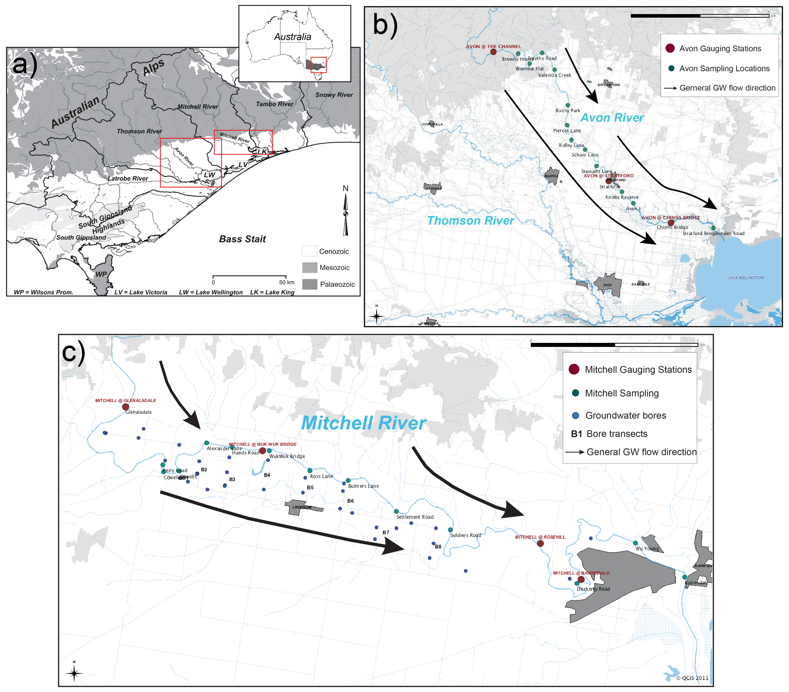
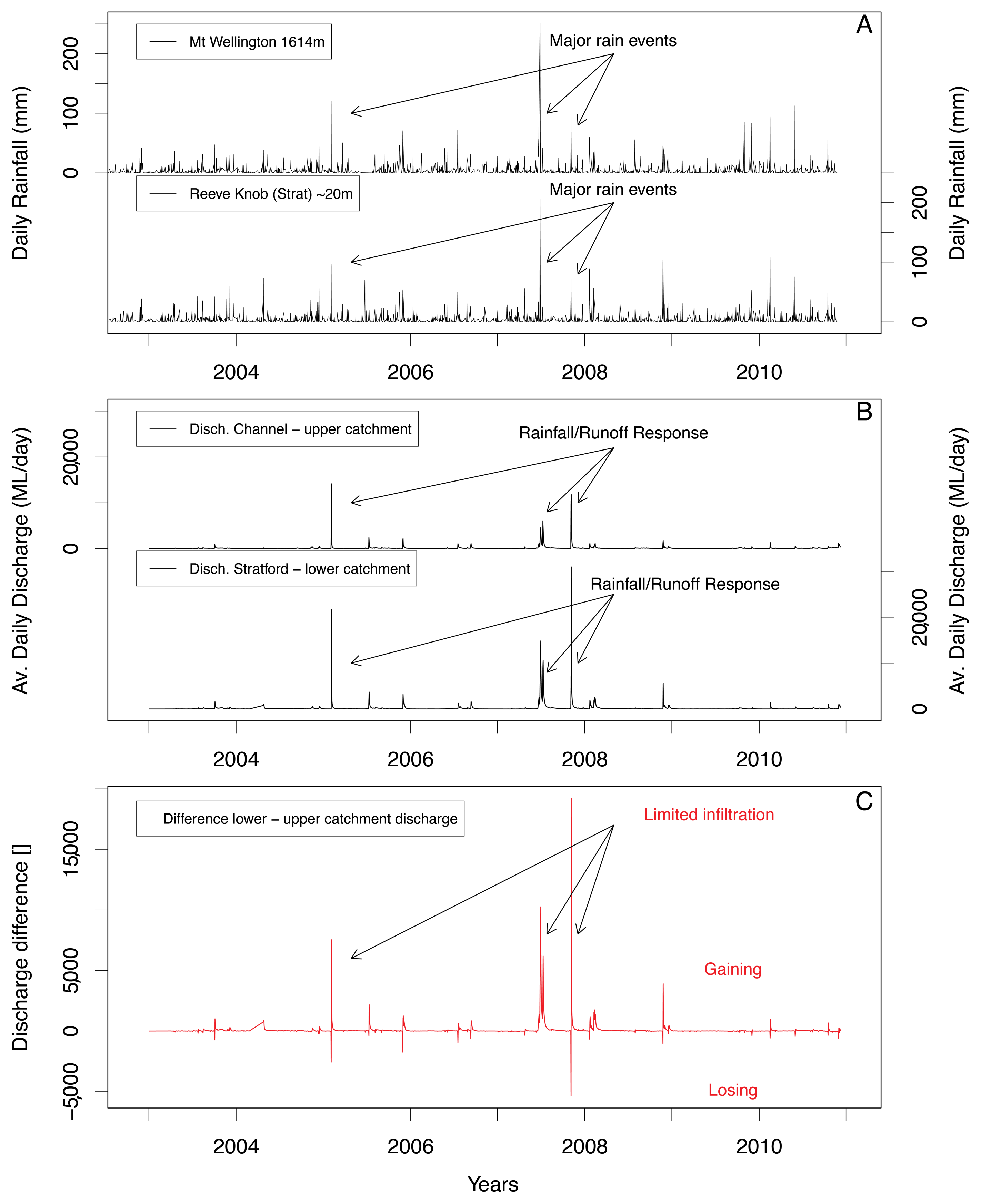
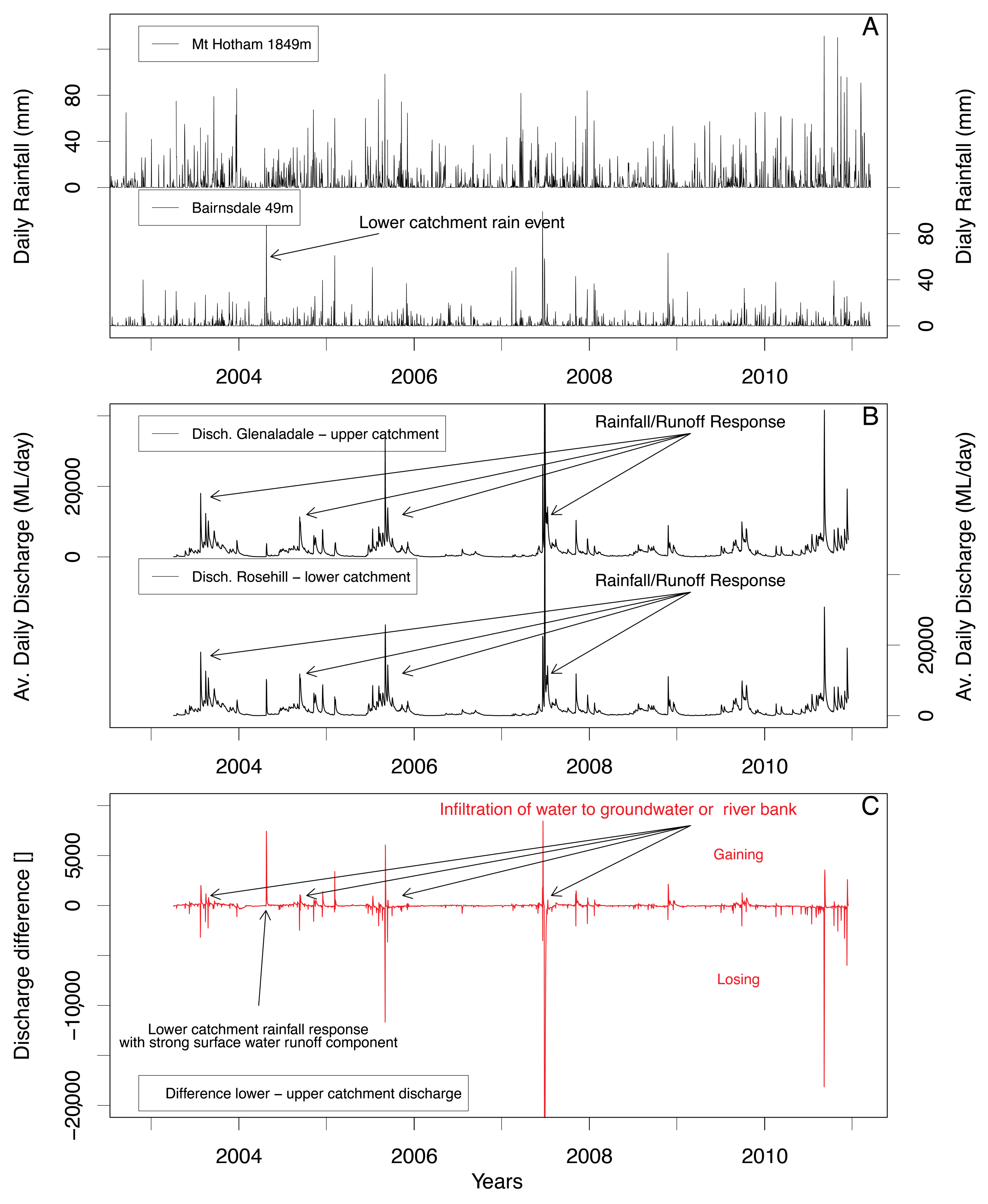
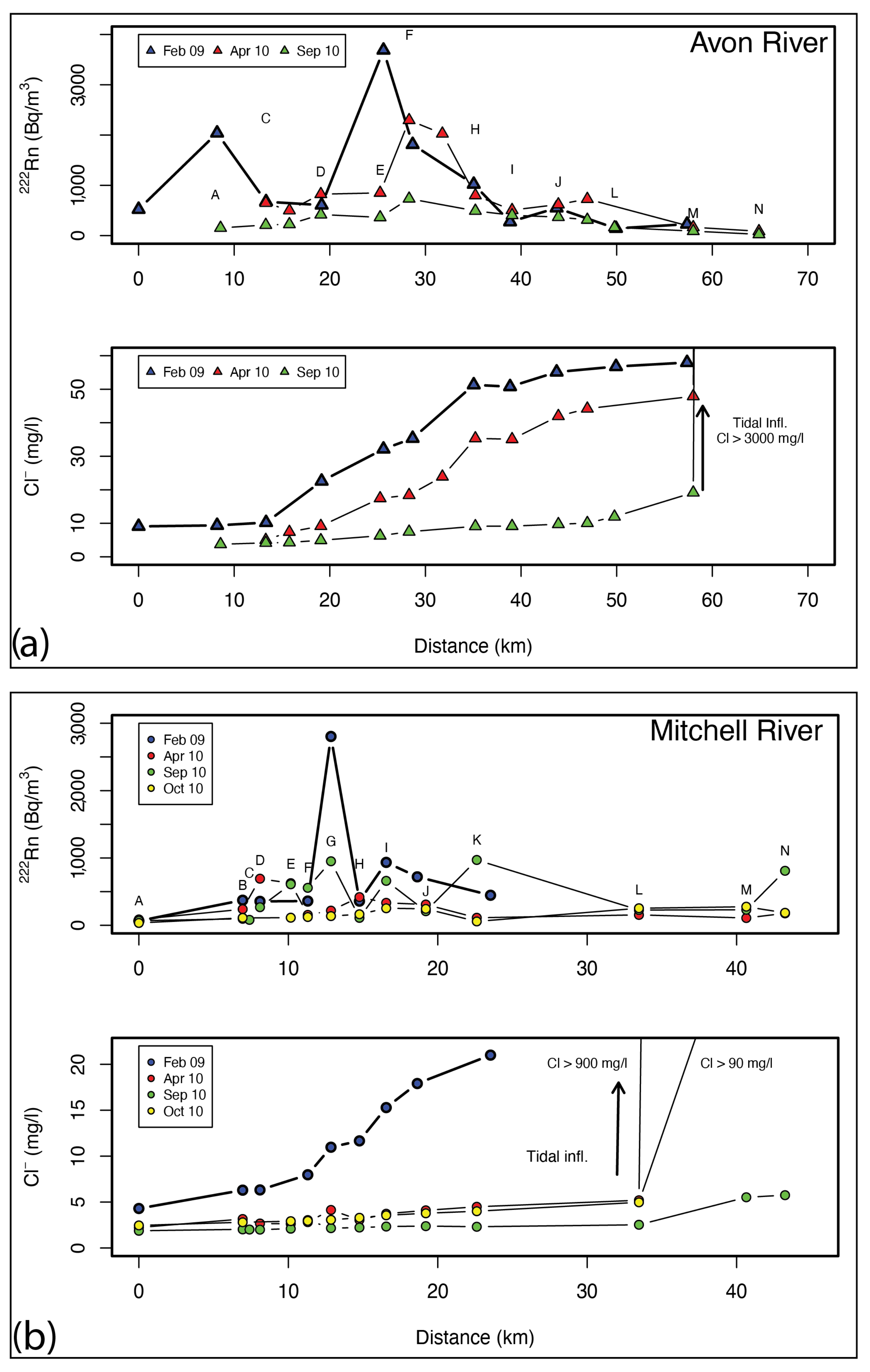
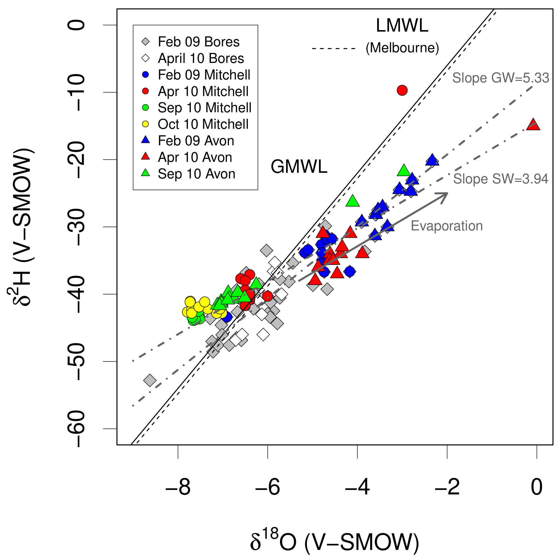
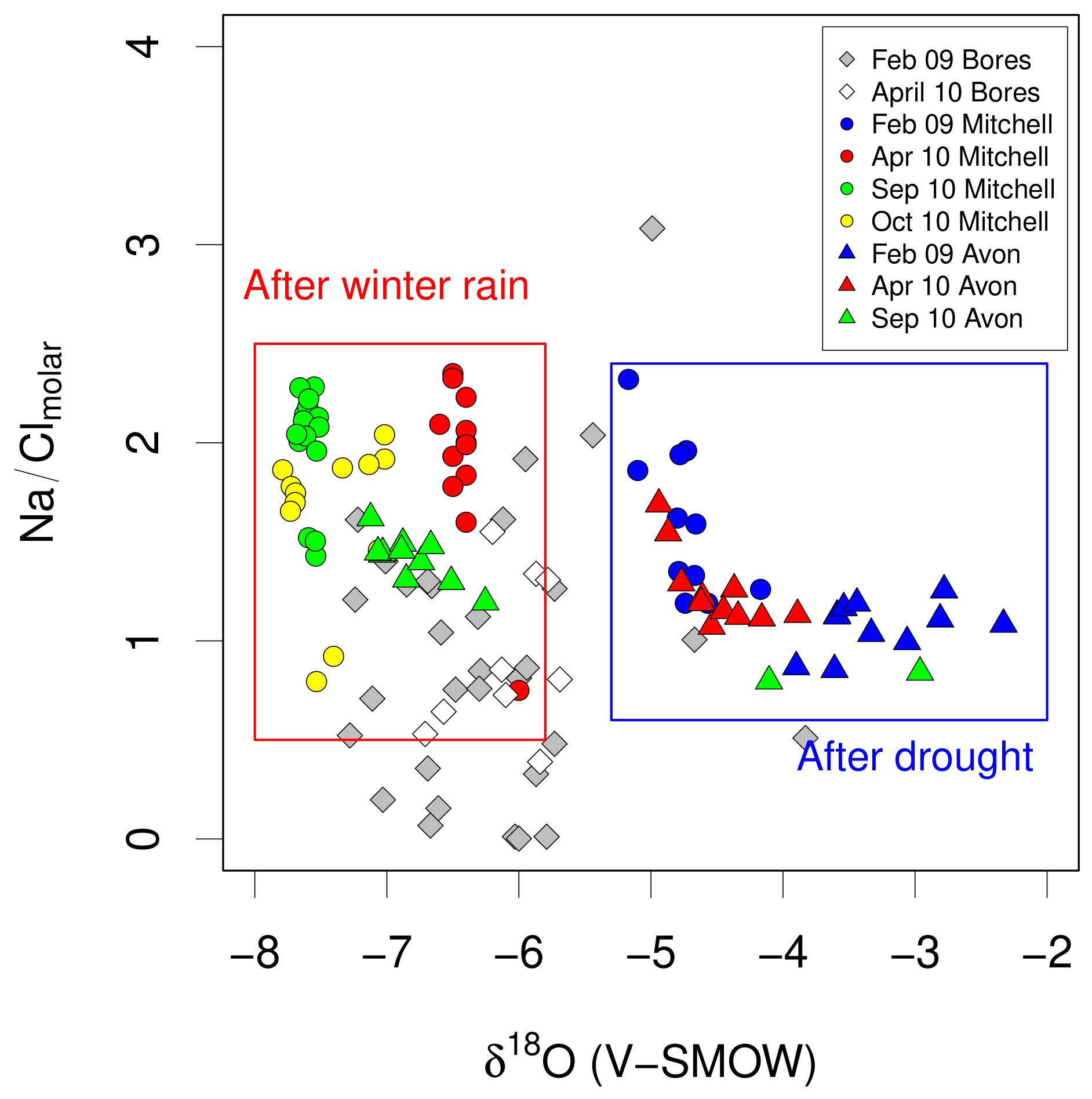
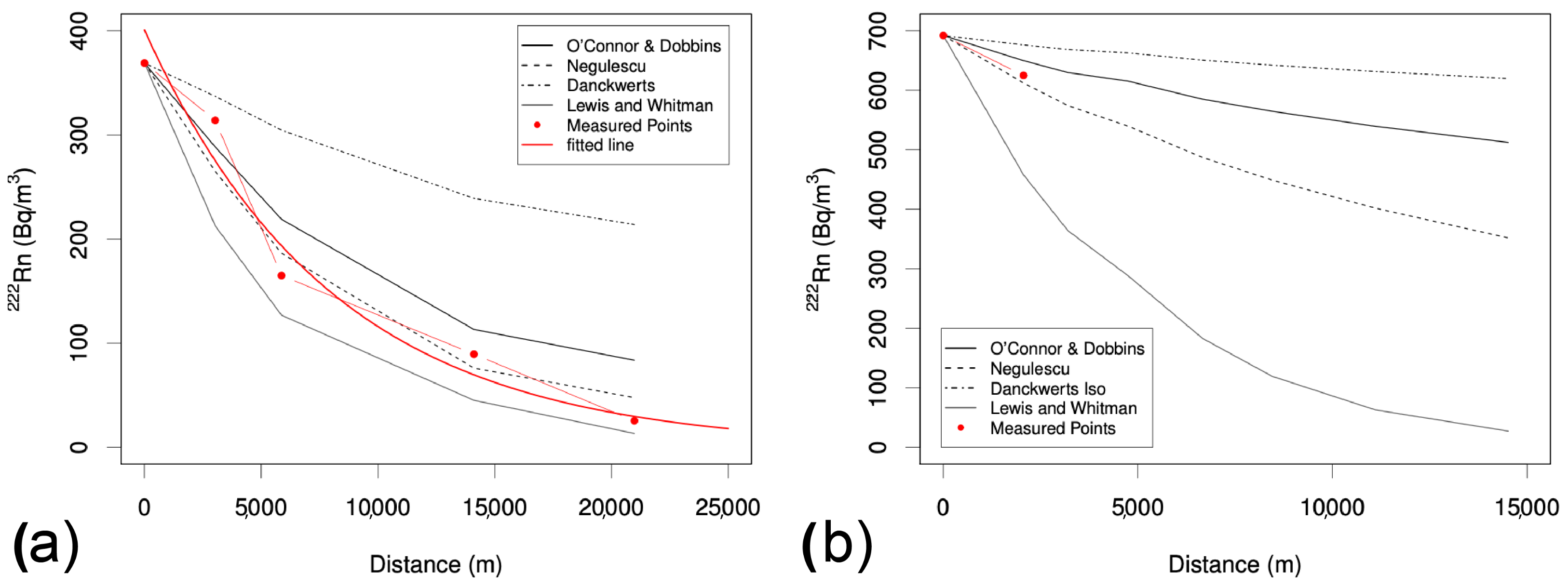
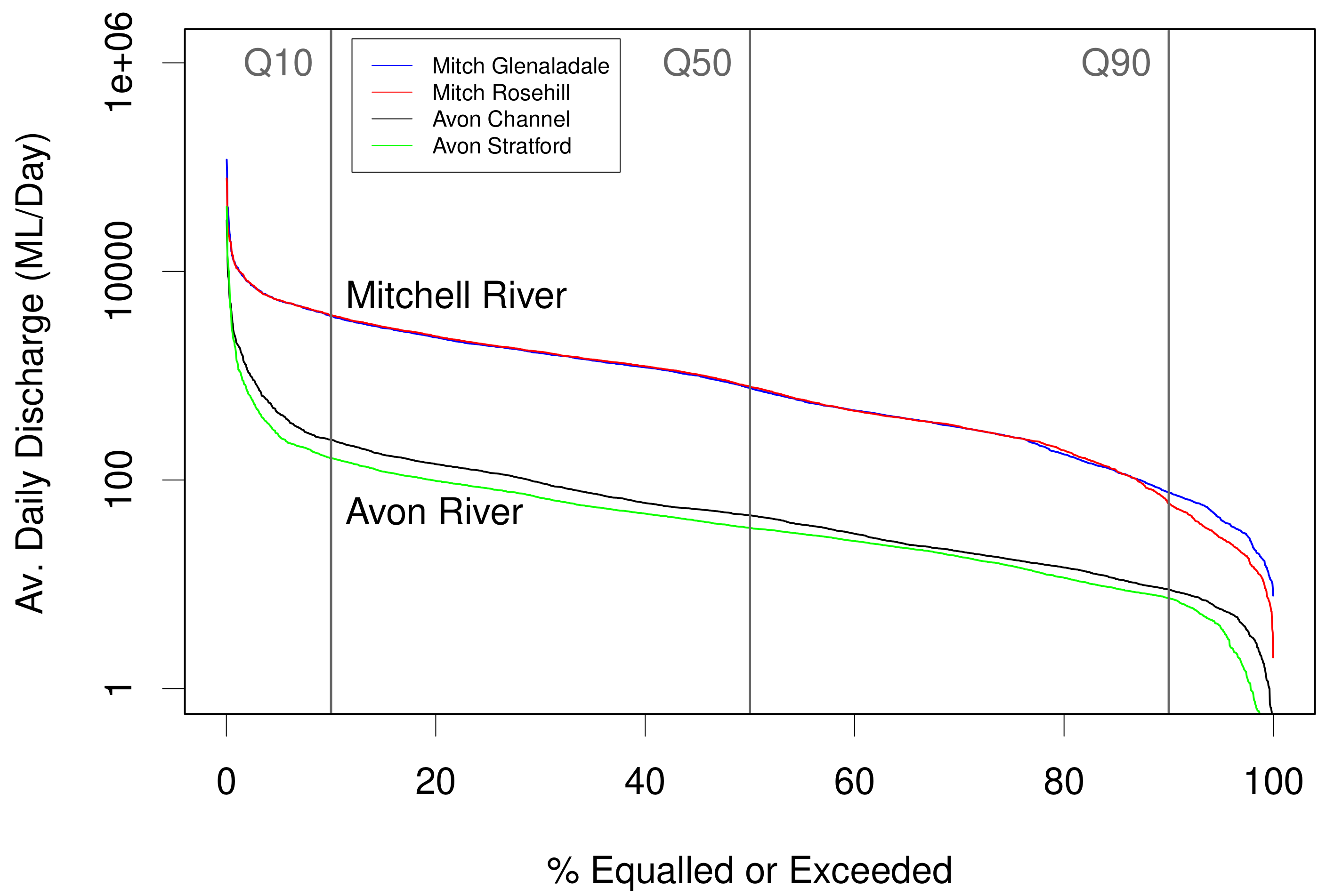
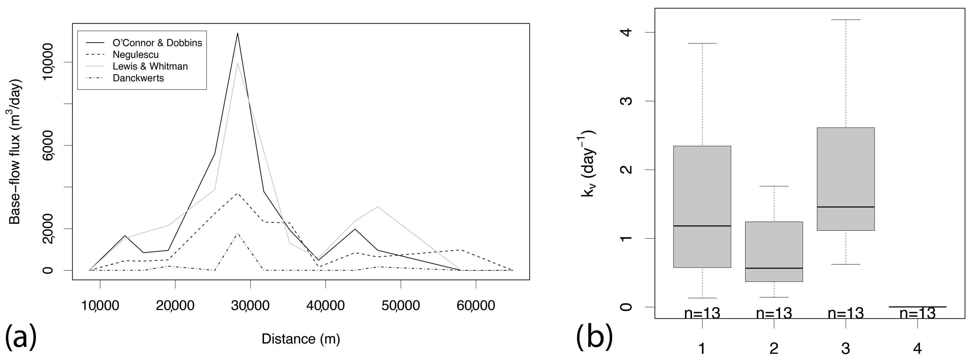
Table A1.
Sensitivity analysis for groundwater Rn and Cl concentrations in groundwater.
| Radon | Baseflow Flux | Baseflow Flux | Chloride | Baseflow Flux | Baseflow Flux | |
|---|---|---|---|---|---|---|
| mBq m | m d | % | mg L | m d | % | |
| Minimum | 306 | 93,840.00 | 147.69 | 4.9 | 151.62 | 0.24 |
| 1st Qu | 2215 | 219,608.62 | 345.64 | 60 | 42,041.72 | 66.17 |
| Median | 9547 | 22,469.30 | 35.36 | 112 | 11,952.75 | 18.81 |
| Mean | 13,780 | 14,625.74 | 23.02 | 210 | 5284.92 | 8.32 |
| 3rd Qu | 13,700 | 7887.91 | 12.41 | 193 | 5847.10 | 9.20 |
| Maximum | 39,850 | 4383.00 | 6.90 | 2018 | 473.54 | 0.75 |
| Minimum | 607 | 104,801.40 | 164.95 | 8 | 78,954.16 | 124.27 |
| 1st Qu | 2765 | 93,054.47 | 146.46 | 63 | 36,096.86 | 56.81 |
| Median | 10,169 | 20,879.79 | 32.86 | 122 | 105,74.58 | 16.64 |
| Mean | 14,165 | 14,368.82 | 22.62 | 167 | 6986.02 | 11.00 |
| 3rd Qu | 24,105 | 16,206.39 | 25.51 | 187 | 6075.42 | 9.56 |
| Maximum | 33,382 | 5368.63 | 8.45 | 841 | 1161.60 | 1.83 |
| 10 Per. Mean | 12,178.00 | 12,834.55 | 20.20 | 223.70 | 4683.13 | 7.37 |
| 20 Per. Mean | 10,432.00 | 20,273.85 | 31.91 | 266.00 | 4015.68 | 7.37 |
| 30 Per. Mean | 10,151.00 | 20,922.60 | 32.93 | 318.49 | 3278.86 | 5.16 |
| 40 Per. Mean | 9007.00 | 48,167.38 | 75.81 | 347.95 | 2972.94 | 4.68 |
Table A2.
Bore identification numbers, locations, the formation that are tapped, total depth, and screened section for the bores in the Mitchell plain (Data retrieved from the DSE Victorian Water Resources Data Warehouse. Coordinates given are for GDA94 projection. Distances are measured as closest distance to the River. Bore 111800 is close to the Wentworth River (a tributary to the Mitchell further upstream of the Mitchell plains in the mountains).
| Bore ID | Zone 55 | Zone 55 | Formation | Total | Min. Screen | Max. Screen | Distance to |
|---|---|---|---|---|---|---|---|
| Easting | Northing | Depth (m) | Depth (m) | Depth (m) | River (m) | ||
| Mitchell R. | |||||||
| B105392 | 533,546.77 | 5,819,040.87 | Haunted Hills | 30.48 | 22.25 | 25.9 | 887 |
| B105476 | 535,250.04 | 5,818,757.04 | Haunted Hills | 15 | 6 | 12 | 370 |
| B105477 | 534,663.30 | 5,818,097.94 | Haunted Hills | 13 | 2.5 | 8.5 | 100 |
| B105478 | 532,174.27 | 5,819,232.81 | Latrobe Valley | 80 | 47.55 | 62.8 | 415 |
| B105479 | 532,177.63 | 5,819,248.46 | Alluvium | 34 | 13 | 28 | 407 |
| B105480 | 544,361.65 | 5,815,254.82 | Haunted Hills | 13 | 3 | 9 | 639 |
| B110165 | 542,495.67 | 5,815,901.64 | Haunted Hills | 13 | 4 | 10 | 1280 |
| B110177 | 533,766.36 | 5,819,424.67 | Latrobe Valley | 64 | 39 | 42 | 1094 |
| B110978 | 532,125.88 | 5,819,256.26 | Latrobe Valley | 74.5 | 51.5 | 56.5 | 378 |
| B110979 | 536,007.00 | 5,817555.00 | Haunted Hills | 14 | 7 | 13 | 776 |
| B111800 | 536,007.12 | 5,817,555.01 | Latrobe Valley | 108.5 | 58 | 73.5 | NA |
| B140279 | 547,251.10 | 5,813,471.72 | Alluvium | 10.5 | 5 | 9 | 963 |
| B140281 | 551,616.33 | 5,813,146.87 | Alluvium | 17 | 11 | 16 | 364 |
| B56528 | 543,527.55 | 5,815,296.52 | Alluvium | 9.14 | 2.43 | 8.53 | 830 |
| B56529 | 543,606.00 | 5,815,859.00 | Alluvium | 12.19 | 7.01 | 10.79 | 260 |
| B56530 | 543,446.96 | 5,814,801.54 | Alluvium | 7.62 | 3.65 | 7.62 | 1330 |
| B56531 | 540,429.49 | 5,816,748.18 | Alluvium | 9.14 | 3.35 | 8.53 | 1020 |
| B56532 | 540,532.95 | 5,817,382.06 | Alluvium | 6.09 | 3.65 | 6.09 | 390 |
| B56533 | 538,790.13 | 5,816,888.64 | Alluvium | 5.48 | 3.04 | 5.18 | 1720 |
| B56534 | 538,900.00 | 5,817,567.00 | Alluvium | 9.14 | 1.52 | 5.18 | 1010 |
| B56535 | 538,983.63 | 5,818,113.26 | Alluvium | 6.09 | 3.35 | 6.09 | 475 |
| B56536 | 537,168.28 | 5,817,065.98 | Alluvium | 6.4 | 3.65 | 5.48 | 1620 |
| B56537 | 537,253.70 | 5,817,597.20 | Alluvium | 8.84 | 4.57 | 8.83 | 1040 |
| B56538 | 537,358.10 | 5,818,228.16 | Alluvium | 8.22 | 4.57 | 8.22 | 440 |
| B56539 | 536,090.28 | 5,818,069.47 | Alluvium | 6.4 | 5.48 | 6.4 | 390 |
| B56540 | 536,004.43 | 5,817,543.67 | Alluvium | 6.26 | 2.74 | 6.09 | 930 |
| B56541 | 535,280.26 | 5,817,366.23 | Alluvium | 8.84 | 260 | ||
| B56546 | 535,307.58 | 5,817,352.47 | Alluvium | 16 | 4.6 | 10.8 | 320 |
| B56547 | 535,617.48 | 5,817,211.60 | Alluvium | 13 | 6 | 12.6 | 605 |
| B56548 | 536,000.03 | 5,817,513.76 | Alluvium | 12.5 | 5.7 | 12.2 | 770 |
| B56549 | 536,431.10 | 5,816,879.87 | Alluvium | 12 | 5.65 | 12 | 1550 |
| B56550 | 537,262.40 | 5,817,625.36 | Alluvium | 13 | 6 | 12.5 | 1040 |
| B56551 | 537,161.16 | 5,817,037.97 | Alluvium | 14 | 6.8 | 13.2 | 1620 |
| B56552 | 541,992.68 | 5,816,076.16 | Alluvium | 10 | 2 | 8.35 | 1130 |
| B56553 | 542,109.82 | 5,816,820.05 | Alluvium | 11 | 2.5 | 9 | 380 |
| B56744 | 542,151.80 | 5,817,128.18 | Haunted Hills | 12 | 3.5 | 9.5 | 60 |
| B80760 | 545,753.20 | 5,814,007.51 | Alluvium | 6.4 | 1.82 | 5.79 | 550 |
| B80761 | 545,917.80 | 5,814,622.14 | Alluvium | 9.14 | 3.96 | 8.22 | 490 |
| B80762 | 546,008.00 | 5,815,253.77 | Alluvium | 6.4 | 2.43 | 3.96 | 595 |
| B80866 | 544,977.66 | 5,815,480.21 | Haunted Hills | 10 | 3 | 7 | 430 |
| Avon R. | |||||||
| B110166 | 506,559.95 | 5,813,840.79 | Alluvium | 16.5 | 5.5 | 11.5 | 7060 |
| B110167 | 506,764.67 | 5,813,738.34 | Alluvium | 14 | 5 | 11 | 7157 |
| B110168 | 506,979.30 | 5,813,603.51 | Alluvium | 14 | 5.5 | 11.5 | 7290 |
| B110171 | 503,950.26 | 5,811,868.86 | Alluvium | 12 | 5.5 | 8.5 | 3760 |
| B110172 | 503,684.46 | 5,811,915.97 | Alluvium | 44 | 2.5 | 6.5 | 3560 |
Table A3.
Yearly discharge values calculated for the gauging station The Channel and Stratford at the Avon. The downstream discharge is corrected for 20% irrigation extraction. The last two columns represent the total amount of river water gained (positive) and lost (negative) in between the two stations. Two major tributaries, the Freestone and the Valencia Creek, join the Avon River in between the gauging station. The water amounts from the tributaries are subtracted from the discharge at Stratford.
| Avon R. | |||||||
|---|---|---|---|---|---|---|---|
| Year | Q The Channel | Q Stratford | Q Stratford | Q Valencia | Q Freestone | Difference | Difference |
| (ML y) | (ML y) | (Extr. Corr. 20%) | Cr. (ML y) | Cr. (ML y) | (ML y) | (Extr. Corr.) | |
| 2003 | 16,560.7 | 26,754.3 | 32,105.2 | 3008.0 | 2993.9 | 4191.6 | 9542.5 |
| 2004 | 14,679.6 | 24,608.3 | 29,530.0 | 4079.1 | 6215.1 | −365.5 | 4556.2 |
| 2005 | 53,144.6 | 85,737.0 | 102,884.4 | 149,11.2 | 159,92.7 | 1688.6 | 18,836.0 |
| 2006 | 18,212.0 | 29,517.7 | 35,421.3 | 4551.5 | 3470.0 | 3284.3 | 9187.8 |
| 2007 | 92,915.3 | 183,749.6 | 220,499.6 | 71,291.0 | 108,309.8 | −88,766.4 | −52016.5 |
| 2008 | 37,488.2 | 74,120.0 | 89,027.9 | 14,898.0 | 21,722.4 | 11.4 | 14919.4 |
| 2009 | 12,851.3 | 13,265.2 | 15,918.2 | 2967.2 | 1823.7 | −4377.0 | −1724.0 |
| 2010 | 32,532.1 | 38,215.6 | 45,876.9 | 7501.1 | 9212.8 | −11,030.4 | −3369.1 |
Table A4.
Yearly discharge values calculated for the gauging station “Glenaladale” and “Rosehill” along the Mitchell River. The downstream discharge is corrected for 5% for the Mitchell. The last two columns represent the the total amount gained (positive) or lost (negative) at the downstream station.
| Mitchell River | |||||
|---|---|---|---|---|---|
| Year | Q Glenaladale | Q Rosehill | Q Rosehill | Difference | Difference |
| (ML y) | (ML y) | (Extraction Corr. 5%) | (Extraction Corr.) | ||
| 2004 | 525,576.0 | 544,578.9 | 571,807.8 | 19,002.9 | 46,231.8 |
| 2005 | 743,244.8 | 707,909.5 | 707,909.5 | −35,335.3 | 60.2 |
| 2006 | 122,620.0 | 112,478.4 | 118,102.3 | −10,141.6 | −4517.7 |
| 2007 | 928,374.2 | 806,524.4 | 846,850.6 | −121,849.9 | −81,523.6 |
| 2008 | 399,924.1 | 400,635.1 | 420,666.9 | 711.0 | 20,742.8 |
| 2009 | 442,722.0 | 437,898.6 | 459,793.5 | −4832.5 | 17,071.5 |
| 2010 | 905,612.3 | 824,233.4 | 865,445.1 | −81,378.9 | −400,167.2 |
Table A5.
Chemistry results Avon River.
| Site Name | Distance | Lon | Lat | EC | T | pH | F | Cl | Br | NO | SO | HCO | Ba | Ca | Fe | K |
|---|---|---|---|---|---|---|---|---|---|---|---|---|---|---|---|---|
| (km) | (S cm) | (C) | (mg L) | (mg L) | (mg L) | (mg L) | (mg L) | (mg L) | (mg L) | (mg L) | (mg L) | (mg L) | ||||
| February 2009 | ||||||||||||||||
| The Channel | 0 | 146.92629 | −37.80473 | 90.9 | 22 | 7.94 | 0.06 | 9.08 | 0.03 | 0.03 | 1.19 | 5.00 | 0.01 | 6.49 | 0.11 | 1.33 |
| Browns House | 8.21 | 146.94689 | −37.81662 | 98 | 24.7 | 7.64 | 0.07 | 9.38 | 0.87 | 0.02 | 1.22 | 29.00 | 0.01 | 6.09 | 0.17 | 1.35 |
| Wombat Flat | 13.3 | 146.945553 | −37.816774 | 95.5 | 23.1 | 7.74 | 0.06 | 10.23 | 0.69 | 0.04 | 1.25 | 36.00 | 0.01 | 6.03 | 0.19 | 1.40 |
| Valencia Creek | 19.06 | 146.986401 | −37.825054 | 159.4 | 22.3 | 7.51 | 0.07 | 22.57 | 1.37 | 0.11 | 8.75 | 43.00 | 0.02 | 8.31 | 0.21 | 1.55 |
| Bushy Park | 25.26 | 147.008397 | −37.871086 | 184.1 | 22.5 | 7.28 | 0.06 | 32.14 | 1.81 | 0.19 | 10.43 | 34.00 | 0.02 | 8.05 | 0.12 | 1.84 |
| Pierces Lane | 28.29 | 147.007054 | −37.897158 | 212 | 22.3 | 7.65 | 0.06 | 35.34 | 2.47 | 0.96 | 15.04 | 38.00 | 0.03 | 9.42 | 2.06 | |
| School Lane | 35.22 | 147.036527 | −37.929029 | 283 | 24.2 | 7.58 | 0.07 | 51.31 | 3.15 | 0.05 | 14.23 | 41.00 | 0.03 | 9.43 | 2.30 | |
| Stewarts Lane | 39.06 | 147.055492 | −37.950082 | 295 | 24.1 | 7.72 | 0.13 | 50.76 | 3.17 | 0.05 | 22.10 | 46.00 | 0.04 | 10.63 | 3.50 | |
| Stratford | 43.9 | 147.076156 | −37.970044 | 332 | 26 | 7.95 | 0.14 | 55.13 | 3.58 | 0.26 | 24.32 | 53.00 | 0.05 | 11.30 | 4.02 | |
| Redbank Rd | 49.93 | 147.18208 | −38.02224 | 335 | 21.3 | 7.90 | 0.10 | 56.77 | 3.84 | 0.03 | 23.02 | 45.00 | 0.04 | 9.96 | 3.65 | |
| Chinns Bridge | 58.01 | 147.180164 | −38.022914 | 354 | 19.2 | 7.55 | 0.15 | 57.97 | 4.57 | 1.41 | 19.36 | 55.00 | 0.03 | 10.04 | 0.03 | 5.33 |
| April 2010 | ||||||||||||||||
| Wombat Flat | 13.3 | 146.945553 | −37.816774 | 101.7 | 0.05 | 5.02 | 0.02 | 0.07 | 0.94 | 0.01 | 4.90 | 0.07 | 1.13 | |||
| Smyths Road | 15.77 | 146.966165 | −37.803062 | 86.9 | 0.08 | 7.41 | 0.02 | 0.04 | 1.29 | 0.01 | 5.07 | 0.09 | 1.16 | |||
| Valencia Creek Rd | 19.06 | 146.986401 | −37.825054 | 109.8 | 0.08 | 9.18 | 0.03 | 0.08 | 2.82 | 0.02 | 5.92 | 0.11 | 1.26 | |||
| Bushy Park | 25.26 | 147.008397 | −37.871086 | 141.7 | 0.08 | 17.45 | 0.04 | 0.13 | 5.02 | 0.02 | 5.70 | 0.07 | 1.40 | |||
| Pearces Lane | 28.29 | 147.007054 | −37.897158 | 152.6 | 0.07 | 18.42 | 0.07 | 0.42 | 5.93 | 0.02 | 6.32 | 0.04 | 1.50 | |||
| Ridley’s Lane | 31.77 | 147.01 | −37.92 | 184.6 | 0.06 | 23.91 | 0.07 | 0.69 | 7.74 | 0.02 | 6.98 | 0.15 | 1.57 | |||
| School’s Lane | 35.22 | 147.036527 | −37.929029 | 218 | 0.10 | 35.34 | 0.09 | 0.26 | 8.44 | 0.02 | 6.97 | 0.06 | 1.73 | |||
| Stewarts Lane | 39.06 | 147.055492 | −37.950082 | 239 | 0.11 | 35.08 | 0.11 | 0.05 | 14.03 | 0.03 | 7.32 | 0.07 | 2.06 | |||
| Stratford | 43.9 | 147.076156 | −37.970044 | 259 | 0.13 | 41.98 | 0.11 | 0.06 | 14.71 | 0.03 | 7.87 | 0.07 | 2.41 | |||
| Knobs Reserve | 46.93 | 147.097045 | −37.983573 | 372 | 0.14 | 44.20 | 0.12 | 0.17 | 14.73 | 0.04 | 7.93 | 0.06 | 2.47 | |||
| Chinns Bridge | 58.01 | 147.180164 | −38.022914 | 280 | 0.14 | 47.91 | 0.13 | 0.16 | 13.41 | 0.03 | 7.26 | 3.01 | ||||
| Springberg Lane | 64.88 | 147.247886 | −38.030347 | 15,600 | 0.40 | 4833.05 | 23.20 | 1.20 | 926.55 | 142.64 | 0.14 | 168.24 | ||||
| September 2010 | ||||||||||||||||
| Browns House | 8.57 | 146.92663 | −37.804165 | 53.9 | 13 | 0.04 | 3.75 | 0.01 | 0.13 | 0.91 | 0.01 | 3.38 | 0.03 | 0.56 | ||
| Wombat Flat | 13.3 | 146.945553 | −37.816774 | 53 | 11.9 | 0.05 | 4.16 | 0.01 | 0.02 | 1.01 | 0.01 | 3.33 | 0.04 | 0.56 | ||
| Smyths Road | 15.77 | 146.966165 | −37.803062 | 55.3 | 11.8 | 0.05 | 4.29 | 0.00 | 0.01 | 1.04 | 0.00 | 3.38 | 0.04 | 0.57 | ||
| Valencia Creek | 19.06 | 146.986401 | −37.825054 | 63.2 | 13.8 | 0.04 | 4.94 | 0.01 | 0.03 | 1.38 | 0.01 | 3.79 | 0.09 | 0.60 | ||
| Bushy Park | 25.26 | 147.008397 | −37.871086 | 74.2 | 14.5 | 0.05 | 6.30 | 0.02 | 0.03 | 1.95 | 0.01 | 3.63 | 0.08 | 0.73 | ||
| Pierces Lane | 28.29 | 147.007054 | −37.897158 | 77.5 | 14.4 | 0.06 | 7.48 | 0.01 | 0.05 | 2.35 | 0.01 | 3.73 | 0.08 | 0.75 | ||
| School Lane | 35.22 | 147.036527 | −37.929029 | 89.6 | 13.6 | 0.06 | 9.11 | 0.01 | 0.11 | 2.89 | 0.01 | 3.97 | 0.12 | 0.79 | ||
| Stewarts Lane | 39.06 | 147.055492 | −37.950082 | 97.8 | 14.5 | 0.06 | 9.16 | 0.02 | 0.02 | 3.57 | 0.01 | 4.13 | 0.15 | 0.89 | ||
| Stratford | 43.9 | 147.076156 | −37.970044 | 103 | 11.2 | 0.05 | 9.73 | 0.02 | 0.01 | 3.90 | 0.01 | 4.24 | 0.18 | 0.97 | ||
| Knobs Reserve | 46.93 | 147.097045 | −37.983573 | 104.1 | 12.6 | 0.06 | 10.06 | 0.02 | 0.05 | 3.92 | 0.01 | 4.24 | 0.18 | 0.99 | ||
| Redbank Road | 49.77 | 147.115774 | −37.998641 | 106 | 12.4 | 0.06 | 11.97 | 0.03 | 0.02 | 4.40 | 0.01 | 4.24 | 0.16 | 1.00 | ||
| Chinns Bridge | 58.01 | 147.180164 | −38.022914 | 142 | 12.8 | 0.07 | 19.16 | 0.05 | 0.02 | 5.05 | 0.01 | 4.72 | 0.15 | 1.37 | ||
| Springberg | 64.88 | 147.247886 | −38.030347 | 11,500 | 12.2 | 0.39 | 3420.71 | 11.28 | 10.76 | 473.65 | 0.02 | 64.79 | 71.06 | |||
| Stratfieldsaye | 67.97 | 147.286877 | −38.042783 | >30,000 | 0.93 | 4940.82 | 16.94 | 6.79 | 747.70 | 0.03 | 90.62 | 105.45 |
Table A6.
Chemistry results Avon River, continued.
| Site Name | Mg | Na | Si | Sr | Na/Cl | Cl/Br | K/Cl | Ca/Mg | Na/Ca | Ca/Cl | Mg/Cl | O | H | C | Rn | I |
|---|---|---|---|---|---|---|---|---|---|---|---|---|---|---|---|---|
| (mg L) | (mg L) | (mg L) | (mg L) | (molar) | (molar) | (molar) | (molar) | (molar) | (molar) | (molar) | (Bq m) | (g L) | ||||
| February 2009 | ||||||||||||||||
| The Channel | 3.38 | 6.63 | 2.51 | 1.13 | 903.73 | 0.13 | 1.17 | 1.78 | 0.63 | 0.54 | −3.59 | −28.15 | −12.03 | 523.00 | 2.45 | |
| Browns House | 3.62 | 6.76 | 2.40 | 1.11 | 675.05 | 0.13 | 1.02 | 1.93 | 0.57 | 0.56 | −2.81 | −24.74 | −10.42 | 2041.00 | 2.07 | |
| Wombat Flat | 3.80 | 7.19 | 2.33 | 1.08 | 713.21 | 0.12 | 0.96 | 2.09 | 0.52 | 0.54 | −2.33 | −20.25 | −10.96 | 674.38 | 4.18 | |
| Valencia Creek | 5.89 | 14.59 | 2.39 | 1.00 | 801.39 | 0.06 | 0.86 | 3.06 | 0.32 | 0.38 | −3.06 | −24.48 | −11.92 | 607.88 | 2.44 | |
| Bushy Park | 6.86 | 17.81 | 2.05 | 0.85 | 738.74 | 0.05 | 0.71 | 3.86 | 0.22 | 0.31 | −3.61 | −31.34 | −12.88 | 3688.75 | 2.28 | |
| Pierces Lane | 8.68 | 19.90 | 1.83 | 0.87 | 771.63 | 0.05 | 0.66 | 3.69 | 0.24 | 0.36 | −3.90 | −29.29 | −12.66 | 1812.50 | 2.38 | |
| School Lane | 9.96 | 34.51 | 1.91 | 1.04 | 622.20 | 0.04 | 0.57 | 6.39 | 0.16 | 0.28 | −3.33 | −30.01 | −12.11 | 1021.25 | 5.44 | |
| Stewarts Lane | 10.55 | 37.06 | 1.64 | 1.12 | 654.64 | 0.06 | 0.61 | 6.08 | 0.18 | 0.30 | −3.59 | −28.18 | −11.97 | 274.88 | 4.08 | |
| Stratford | 10.76 | 41.74 | 1.82 | 1.17 | 643.64 | 0.07 | 0.64 | 6.44 | 0.18 | 0.28 | −3.54 | −27.49 | −11.90 | 550.00 | 5.42 | |
| Redbank Rd | 10.91 | 43.83 | 1.20 | 1.19 | 652.35 | 0.06 | 0.55 | 7.69 | 0.15 | 0.28 | −3.44 | −27.05 | −12.32 | 143.38 | 9.78 | |
| Chinns Bridge | 11.00 | 47.24 | 0.77 | 1.26 | 557.31 | 0.08 | 0.55 | 8.22 | 0.15 | 0.28 | −2.78 | −23.06 | −11.48 | 228.25 | 12.47 | |
| April 2010 | ||||||||||||||||
| Wombat Flat | 2.94 | 5.41 | 1.72 | 0.02 | 1.69 | 473.33 | 0.21 | 1.02 | 1.97 | 0.26 | 0.85 | −4.94 | −38.00 | 650.00 | ||
| Smyths Road | 3.10 | 6.23 | 1.59 | 0.02 | 1.29 | 696.67 | 0.14 | 0.98 | 2.13 | 0.34 | 0.62 | −4.77 | −31.00 | 502.00 | ||
| Valencia Creek Rd | 3.81 | 9.13 | 1.87 | 0.03 | 1.54 | 647.50 | 0.12 | 0.93 | 2.70 | 0.41 | 0.62 | −4.87 | −36.00 | 825.00 | ||
| Bushy Park | 4.97 | 13.79 | 1.56 | 0.03 | 1.22 | 984.00 | 0.08 | 0.68 | 4.23 | 0.63 | 0.43 | −4.61 | −34.00 | 850.00 | ||
| Pearces Lane | 5.61 | 14.21 | 1.68 | 0.03 | 1.19 | 577.78 | 0.08 | 0.69 | 3.92 | 0.68 | 0.44 | −4.62 | −35.00 | 2296.00 | ||
| Ridley’s Lane | 6.60 | 19.52 | 1.87 | 0.04 | 1.26 | 748.89 | 0.06 | 0.64 | 4.89 | 0.85 | 0.40 | −4.37 | −34.00 | 2028.00 | ||
| School’s Lane | 7.05 | 24.51 | 1.95 | 0.04 | 1.07 | 906.36 | 0.04 | 0.60 | 6.15 | 1.17 | 0.29 | −4.54 | −35.00 | 801.00 | ||
| Stewarts Lane | 7.32 | 26.19 | 1.76 | 0.04 | 1.15 | 706.43 | 0.05 | 0.61 | 6.23 | 1.17 | 0.30 | −4.45 | −37.00 | 508.00 | ||
| Stratford | 7.71 | 30.50 | 1.85 | 0.05 | 1.12 | 845.71 | 0.05 | 0.61 | 6.79 | 1.38 | 0.27 | −4.34 | −33.00 | 620.00 | ||
| Knobs Reserve | 7.86 | 31.85 | 1.71 | 0.05 | 1.11 | 831.33 | 0.05 | 0.62 | 7.02 | 1.45 | 0.26 | −4.16 | −31.00 | 728.00 | ||
| Chinns Bridge | 7.94 | 35.08 | 0.69 | 0.05 | 1.13 | 844.38 | 0.06 | 0.55 | 8.45 | 1.53 | 0.24 | −3.89 | −34.00 | 167.00 | ||
| Springberg Lane | 494.28 | 4062.29 | 4.45 | 2.70 | 1.30 | 469.59 | 0.03 | 0.17 | 49.65 | 0.15 | −0.08 | −15.00 | 87.00 | |||
| September 2010 | ||||||||||||||||
| Browns House | 1.84 | 3.94 | 2.20 | 0.01 | 1.62 | 931.19 | 0.14 | 1.12 | 2.03 | 0.80 | 0.71 | −7.12 | −41.64 | 153.63 | ||
| Wombat Flat | 1.83 | 3.88 | 2.16 | 0.01 | 1.44 | 970.51 | 0.12 | 1.10 | 2.03 | 0.71 | 0.64 | −7.04 | −41.10 | 212.38 | ||
| Smyths Road | 1.87 | 4.02 | 2.17 | 0.01 | 1.44 | 1964.71 | 0.12 | 1.10 | 2.07 | 0.70 | 0.64 | −7.03 | −41.36 | 226.50 | ||
| Valencia Creek | 2.07 | 4.63 | 2.18 | 0.01 | 1.45 | 1946.25 | 0.11 | 1.11 | 2.13 | 0.68 | 0.61 | −7.07 | −41.71 | 419.64 | ||
| Bushy Park | 2.45 | 6.09 | 1.86 | 0.01 | 1.49 | 648.75 | 0.10 | 0.90 | 2.92 | 0.51 | 0.57 | −6.88 | −39.80 | 363.29 | ||
| Pierces Lane | 2.60 | 6.36 | 1.74 | 0.02 | 1.31 | 1270.81 | 0.09 | 0.87 | 2.98 | 0.44 | 0.51 | −6.85 | −40.65 | 734.56 | ||
| School Lane | 3.02 | 8.27 | 1.48 | 0.02 | 1.40 | 1644.43 | 0.08 | 0.80 | 3.63 | 0.39 | 0.48 | −6.74 | −40.74 | 493.38 | ||
| Stewarts Lane | 3.10 | 8.65 | 1.35 | 0.02 | 1.46 | 964.07 | 0.09 | 0.81 | 3.65 | 0.40 | 0.49 | −6.89 | −40.88 | 405.52 | ||
| Stratford | 3.20 | 9.30 | 1.21 | 0.02 | 1.47 | 1245.93 | 0.09 | 0.80 | 3.83 | 0.39 | 0.48 | −41.32 | 368.98 | |||
| Knobs Reserve | 3.26 | 9.65 | 1.13 | 0.02 | 1.48 | 988.06 | 0.09 | 0.79 | 3.97 | 0.37 | 0.47 | −6.67 | −39.74 | 314.02 | ||
| Redbank Road | 3.36 | 10.08 | 1.11 | 0.02 | 1.30 | 951.84 | 0.08 | 0.77 | 4.14 | 0.31 | 0.41 | −6.51 | −40.55 | 164.92 | ||
| Chinns Bridge | 4.06 | 14.85 | 1.06 | 0.03 | 1.20 | 932.94 | 0.06 | 0.70 | 5.49 | 0.22 | 0.31 | −6.25 | −38.59 | 89.48 | ||
| Springberg | 214.49 | 1767.17 | 2.26 | 1.11 | 0.80 | 683.56 | 0.02 | 0.18 | 47.55 | 0.02 | 0.09 | −4.11 | −26.35 | 25.53 | ||
| Stratfieldsaye | 310.09 | 2694.57 | 3.11 | 1.59 | 0.84 | 657.37 | 0.02 | 0.18 | 51.84 | 0.02 | 0.09 | −2.96 | −21.82 |
Table A7.
Chemistry results Mitchell River.
| Site Name | Distance | Lon | Lat | EC | T | pH | F | Cl | Br | NO | SO | HCO | Ba | Ca | Fe | K |
|---|---|---|---|---|---|---|---|---|---|---|---|---|---|---|---|---|
| (km) | (S cm) | (C) | (mg L) | (mg L) | (mg L) | (mg L) | (mg L) | (mg L) | (mg L) | (mg L) | (mg L) | (mg L) | ||||
| February 2009 | ||||||||||||||||
| Wentworth River | 147.34671 | −37.59451 | 70.5 | 7.52 | 0.07 | 5.09 | 0.00 | 0.27 | 0.96 | 30.00 | ||||||
| Hortan Rd | 147.37146 | −37.63254 | 71.8 | 7.28 | 0.05 | 3.52 | 0.01 | 0.03 | 0.99 | 38.00 | 0.01 | 4.21 | 0.16 | 1.10 | ||
| Jurgenson Pt | 147.37830 | −37.75795 | 90.5 | 7.45 | 0.05 | 4.13 | 0.01 | 0.01 | 1.02 | 13.00 | 0.01 | 4.28 | 0.13 | 1.57 | ||
| Glenaladale | 0.00 | 147.39366 | −37.78322 | 83.6 | 21.10 | 7.51 | 0.07 | 4.30 | 0.01 | 0.03 | 1.00 | 35.00 | 0.01 | 4.38 | 0.07 | 1.21 |
| Perry Rd | 6.94 | 147.40028 | −37.78764 | 90.7 | 0.06 | 6.30 | 0.02 | 0.24 | 1.93 | 14.00 | 0.01 | 4.62 | 1.18 | |||
| Cowells Rd | 8.10 | 147.42623 | −37.77870 | 97.7 | 24.30 | 7.94 | 0.05 | 6.32 | 0.02 | 0.03 | 1.71 | 40.00 | 0.01 | 4.67 | 0.13 | 1.14 |
| Hands Rd | 11.30 | 147.44339 | −37.78001 | 120.6 | 25.70 | 7.35 | 0.07 | 7.98 | 0.04 | 0.79 | 3.17 | 38.00 | 0.01 | 5.05 | 0.24 | 1.21 |
| Wuk Wuk Bridge | 12.85 | 147.46258 | −37.78642 | 122.4 | 23.10 | 7.68 | 0.07 | 10.98 | 0.04 | 0.49 | 5.12 | 55.00 | 0.01 | 5.71 | 0.05 | 1.28 |
| Ross Ln | 14.76 | 147.48009 | −37.79131 | 148.3 | 23.90 | 7.60 | 0.06 | 11.67 | 0.05 | 1.38 | 6.10 | 25.00 | 0.01 | 6.04 | 0.09 | 1.28 |
| Bulmers Ln | 16.55 | 147.49817 | −37.79791 | 157.2 | 22.80 | 7.56 | 0.08 | 15.29 | 0.06 | 2.42 | 8.26 | 38.00 | 0.02 | 7.68 | 1.32 | |
| Settlement Rd | 18.63 | 147.50438 | −37.80299 | 173.9 | 25.40 | 7.69 | 0.07 | 17.91 | 0.06 | 2.60 | 9.12 | 39.00 | 0.02 | 8.18 | 1.35 | |
| Soldiers Rd | 23.53 | 146.85466 | −37.81140 | 90.9 | 22.00 | 7.94 | 0.08 | 21.00 | 0.08 | 2.14 | 9.77 | 53.00 | 0.02 | 8.68 | 0.11 | 1.40 |
| April 2010 | ||||||||||||||||
| Glenaladale | 0.00 | 147.374558 | −37.763447 | 54.5 | 0.04 | 2.23 | 0.00 | 0.82 | 0.92 | 3.40 | 0.64 | 3.20 | 0.19 | |||
| Perry Rd | 6.94 | 147.391433 | −37.784979 | 58.1 | 0.05 | 3.16 | 0.01 | 0.01 | 1.77 | 4.10 | 0.68 | 3.20 | 0.20 | |||
| Cowells Rd | 8.10 | 147.392372 | −37.788664 | 66.1 | 0.04 | 2.67 | 0.01 | 0.00 | 1.05 | 3.60 | 0.64 | 3.20 | 0.20 | |||
| Alexanders Rd | 10.16 | 147.413379 | −37.777166 | 62.9 | 0.06 | 2.63 | 0.00 | 0.03 | 1.23 | 3.80 | 0.66 | 3.30 | 0.20 | |||
| Hands Rd | 11.30 | 147.425513 | −37.778667 | 62.3 | 0.05 | 2.82 | 0.01 | 1.12 | 1.30 | 3.80 | 0.65 | 3.30 | 0.18 | |||
| WukWuk Bridge | 12.85 | 147.443241 | −37.779986 | 63.7 | 0.05 | 4.14 | 0.01 | 0.00 | 2.83 | 5.20 | 0.69 | 3.50 | 0.19 | |||
| Ross Ln | 14.76 | 147.462571 | −37.787356 | 65.6 | 0.03 | 3.06 | 0.01 | 0.03 | 1.63 | 4.60 | 0.69 | 3.50 | 0.21 | |||
| Bulmers Ln | 16.55 | 147.480801 | −37.791039 | 90.5 | 0.04 | 3.73 | 0.01 | 0.11 | 1.99 | 4.80 | 0.70 | 3.60 | 0.22 | |||
| Settlement Rd | 19.20 | 147.503786 | −37.802592 | 72.2 | 0.04 | 4.10 | 0.01 | 0.30 | 2.20 | 4.90 | 0.68 | 3.70 | 0.19 | |||
| Soldiers Rd | 22.61 | 147.529575 | −37.809491 | 71.8 | 0.05 | 4.49 | 0.02 | 0.21 | 2.75 | 5.20 | 0.70 | 3.80 | 0.19 | |||
| Dockertys Rd | 33.46 | 147.589987 | −37.829372 | 72.8 | 0.05 | 5.20 | 0.02 | 0.25 | 2.33 | 5.40 | 0.71 | 4.00 | 0.19 | |||
| Wy Yung Bridge | 40.65 | 147.617858 | −37.813982 | 2500 | 0.08 | 915.41 | 2.57 | 0.27 | 131.66 | 445.00 | 18.00 | 19.00 | 0.06 | |||
| Bairsdale | 43.24 | 147.641422 | −37.826786 | 1687 | 8.28 | 297.66 | 1.56 | 11.19 | 3360.24 | 4633.00 | 186.00 | 147.00 | 0.00 |
Table A8.
Chemistry results Mitchell River, continued.
| Site Name | Distance | Lon | Lat | EC | T | pH | F | Cl | Br | NO | SO | HCO | Ba | Ca | Fe | K |
|---|---|---|---|---|---|---|---|---|---|---|---|---|---|---|---|---|
| (km) | (S cm) | (C) | (mg L) | (mg L) | (mg L) | (mg L) | (mg L) | (mg L) | (mg L) | (mg L) | (mg L) | (mg L) | ||||
| September 2010 | ||||||||||||||||
| D.O. Nargun | 147.286877 | −38.042783 | 39 | 11.90 | 0.03 | 1.93 | 0.00 | 0.46 | 0.80 | 0.01 | 2.05 | 0.05 | 0.65 | |||
| Glenaladale | 0.00 | 147.374558 | −37.763447 | 41 | 15.00 | 7.01 | 0.03 | 1.88 | 0.00 | 0.50 | 0.79 | 0.00 | 1.97 | 0.05 | 0.65 | |
| Perry Road | 6.94 | 147.391433 | −37.784979 | 44.7 | 12.30 | 0.03 | 2.03 | 0.01 | 0.52 | 0.84 | 0.00 | 2.04 | 0.07 | 0.63 | ||
| CowellsB | 7.40 | 147.392372 | −37.788664 | 40.5 | 12.20 | 0.03 | 2.01 | 0.01 | 0.55 | 0.87 | 0.00 | 2.04 | 0.06 | 0.63 | ||
| Cowells | 8.10 | 147.399888 | −37.787553 | 42.3 | 13.50 | 6.22 | 0.03 | 2.00 | 0.00 | 0.52 | 0.86 | 0.00 | 2.03 | 0.06 | 0.64 | |
| Alexander Rd | 10.16 | 147.413379 | −37.777166 | 42.6 | 13.00 | 7.40 | 0.03 | 2.10 | 0.01 | 0.57 | 0.97 | 0.00 | 2.05 | 0.06 | 0.63 | |
| Hands Road | 11.30 | 147.425513 | −37.778667 | 42.5 | 12.50 | 7.37 | 0.03 | 3.03 | 0.01 | 0.57 | 1.13 | 0.00 | 2.00 | 0.06 | 0.63 | |
| WukWuk Bridge | 12.85 | 147.443241 | −37.779986 | 45 | 12.50 | 7.40 | 0.03 | 2.16 | 0.01 | 0.61 | 1.58 | 0.01 | 2.24 | 0.07 | 0.67 | |
| Ross Ln | 14.76 | 147.462571 | −37.787356 | 44 | 12.80 | 0.03 | 2.22 | 0.01 | 0.52 | 1.03 | 0.00 | 2.14 | 0.06 | 0.66 | ||
| Bulmers Ln | 16.55 | 147.480801 | −37.791039 | 42.3 | 12.30 | 7.10 | 0.03 | 2.34 | 0.01 | 0.66 | 1.08 | 0.00 | 2.15 | 0.06 | 0.64 | |
| Settlement Rd | 19.20 | 147.503786 | −37.802592 | 43.3 | 11.80 | 7.40 | 0.03 | 2.39 | 0.02 | 0.61 | 1.10 | 0.00 | 2.17 | 0.06 | 0.66 | |
| Soldiers Rd | 22.61 | 147.529575 | −37.809491 | 44.7 | 11.40 | 7.50 | 0.04 | 2.32 | 0.00 | 0.59 | 1.13 | 0.00 | 2.15 | 0.06 | 0.67 | |
| Dockerty Rd | 33.46 | 147.589987 | −37.829372 | 47.7 | 12.00 | 7.30 | 0.03 | 2.53 | 0.01 | 0.57 | 1.19 | 0.00 | 2.29 | 0.07 | 0.67 | |
| Wu Young | 40.65 | 147.617858 | −37.813982 | 62.4 | 11.40 | 7.11 | 0.03 | 5.52 | 0.02 | 0.59 | 1.57 | 0.00 | 2.42 | 0.07 | 0.77 | |
| Bairnsdale | 43.24 | 147.641422 | −37.826786 | 64.5 | 11.50 | 6.94 | 0.03 | 5.75 | 0.02 | 0.61 | 1.68 | 0.00 | 2.42 | 0.07 | 0.78 | |
| October 2010 | ||||||||||||||||
| Glenaladale | 0.00 | 147.374558 | −37.763447 | 45.6 | 16.20 | 0.04 | 2.46 | 0.00 | 0.00 | 1.09 | 0.00 | 2.50 | 0.13 | 0.60 | ||
| Perry Road | 6.94 | 147.391433 | −37.784979 | 47.3 | 15.90 | 0.04 | 2.81 | 0.01 | 0.00 | 1.23 | 0.00 | 2.57 | 0.14 | 0.60 | ||
| Alexander Rd | 10.16 | 147.413379 | −37.777166 | 48.6 | 16.20 | 0.04 | 2.91 | 0.00 | 0.06 | 1.36 | 0.00 | 2.61 | 0.15 | 0.61 | ||
| Hands Rd | 11.30 | 147.425513 | −37.778667 | 49 | 15.90 | 0.04 | 2.96 | 0.01 | 0.05 | 1.38 | 0.00 | 2.59 | 0.15 | 0.61 | ||
| WukWuk Bridge | 12.85 | 147.443241 | −37.779986 | 50.1 | 16.40 | 0.04 | 3.07 | 0.00 | 0.08 | 1.76 | 0.00 | 2.70 | 0.17 | 0.62 | ||
| Ross Ln | 14.76 | 147.462571 | −37.787356 | 51.4 | 15.90 | 0.04 | 3.29 | 0.01 | 0.07 | 1.68 | 0.00 | 2.71 | 0.16 | 0.62 | ||
| Bulmers Ln | 16.55 | 147.480801 | −37.791039 | 54 | 16.50 | 0.04 | 3.56 | 0.00 | 0.25 | 1.90 | 0.00 | 2.89 | 0.17 | 0.62 | ||
| Settlement Rd | 19.20 | 147.503786 | −37.802592 | 55.1 | 15.70 | 0.04 | 3.78 | 0.01 | 0.20 | 2.01 | 0.01 | 2.97 | 0.18 | 0.63 | ||
| Soldiers Rd | 22.61 | 147.529575 | −37.809491 | 55.5 | 16.00 | 0.03 | 4.01 | 0.01 | 0.16 | 2.06 | 0.00 | 2.91 | 0.20 | 0.63 | ||
| Dockerty Rd | 33.46 | 147.589987 | −37.829372 | 64.9 | 13.90 | 0.04 | 4.98 | 0.01 | 0.21 | 2.13 | 0.01 | 3.28 | 0.23 | 0.64 | ||
| Wu Young | 40.65 | 147.617858 | −37.813982 | 708 | 15.00 | 0.01 | 38.83 | 0.12 | 0.07 | 5.42 | 0.00 | 1.36 | 0.05 | 1.00 | ||
| Bairnsdale | 43.24 | 147.641422 | −37.826786 | 1908 | 15.00 | 0.02 | 98.91 | 0.37 | 0.04 | 14.92 | 0.00 | 2.81 | 0.04 | 2.56 |
Table A9.
Chemistry results Mitchell River, continued.
| Site Name | Mg | Na | Si | Sr | Na/Cl | Cl/Br | K/Cl | Ca/Mg | Na/Ca | Ca/Cl | Mg/Cl | O | H | C | Rn | I |
|---|---|---|---|---|---|---|---|---|---|---|---|---|---|---|---|---|
| (mg L) | (mg L) | (mg L) | (mg L) | (molar) | (molar) | (molar) | (molar) | (molar) | (molar) | (molar) | (Bq m) | (g L) | ||||
| February 2009 | ||||||||||||||||
| Wentworth River | 2810.06 | −6.91 | −43.39 | −11.22 | 0.00 | 3.97 | ||||||||||
| Hortan Rd | 3.61 | 5.30 | 3.17 | 0.04 | 2.32 | 950.77 | 0.28 | 0.71 | 2.19 | 1.06 | 1.49 | −5.17 | −33.83 | −10.35 | 236.36 | 1.96 |
| Jurgenson Pt | 3.65 | 5.00 | 3.13 | 0.04 | 1.86 | 866.25 | 0.34 | 0.71 | 2.04 | 0.92 | 1.29 | −5.10 | −33.42 | −10.17 | 0.00 | 1.65 |
| Glenaladale | 3.63 | 5.47 | 2.91 | 0.04 | 1.96 | 659.31 | 0.25 | 0.73 | 2.18 | 0.90 | 1.23 | −4.73 | −31.18 | −10.08 | 65.68 | 1.79 |
| Perry Rd | 4.03 | 7.92 | 2.88 | 0.04 | 1.94 | 665.65 | 0.17 | 0.70 | 2.99 | 0.65 | 0.93 | −4.78 | −34.95 | −9.97 | 373.75 | 2.41 |
| Cowells Rd | 3.95 | 6.65 | 2.84 | 0.04 | 1.62 | 604.30 | 0.16 | 0.72 | 2.48 | 0.65 | 0.91 | −4.80 | −32.62 | −10.44 | 355.67 | 1.92 |
| Hands Rd | 4.39 | 8.22 | 2.74 | 0.04 | 1.59 | 437.18 | 0.14 | 0.70 | 2.84 | 0.56 | 0.80 | −4.66 | −34.71 | −9.73 | 360.20 | 3.27 |
| Wuk Wuk Bridge | 4.93 | 9.61 | 2.77 | 0.05 | 1.35 | 566.39 | 0.11 | 0.70 | 2.94 | 0.46 | 0.65 | −4.79 | −33.86 | −10.69 | 2803.99 | 2.55 |
| Ross Street | 5.25 | 10.10 | 2.79 | 0.05 | 1.33 | 554.71 | 0.10 | 0.70 | 2.92 | 0.46 | 0.66 | −4.67 | −31.87 | −10.80 | 359.33 | 2.02 |
| Bulmers Rd | 5.83 | 12.49 | 2.87 | 0.07 | 1.26 | 589.26 | 0.08 | 0.80 | 2.84 | 0.44 | 0.56 | −4.17 | −36.64 | −11.54 | 934.69 | 2.69 |
| Settlement Rd | 6.16 | 13.77 | 2.90 | 0.08 | 1.19 | 623.69 | 0.07 | 0.81 | 2.94 | 0.40 | 0.50 | −4.74 | −36.70 | −12.04 | 720.45 | 2.31 |
| Soldiers Rd | 6.39 | 16.17 | 2.78 | 0.08 | 1.19 | 598.18 | 0.06 | 0.82 | 3.25 | 0.37 | 0.44 | −4.57 | −31.77 | −10.74 | 446.41 | 3.00 |
| April 2010 | ||||||||||||||||
| Glenaladale | 2.70 | 2.00 | 2.35 | 0.26 | 0.72 | 1.85 | 1.27 | 1.76 | −6.50 | −40.00 | 87.00 | |||||
| Perry Rd | 2.90 | 2.10 | 2.00 | 890.00 | 0.20 | 0.67 | 2.23 | 0.90 | 1.34 | −6.40 | −37.10 | 239.00 | ||||
| Cowells Rd | 2.70 | 2.00 | 2.09 | 750.00 | 0.22 | 0.72 | 1.97 | 1.06 | 1.48 | −6.60 | −37.70 | 692.00 | ||||
| Alexanders Rd | 2.80 | 2.00 | 2.23 | 0.23 | 0.72 | 2.00 | 1.11 | 1.55 | −6.40 | −40.80 | 625.00 | |||||
| Hands Rd | 2.80 | 2.00 | 2.06 | 800.00 | 0.21 | 0.72 | 2.00 | 1.03 | 1.44 | −6.40 | −39.90 | 155.00 | ||||
| WukWuk Bridge | 3.10 | 2.10 | 1.93 | 1170.00 | 0.15 | 0.68 | 2.59 | 0.75 | 1.09 | −6.50 | −38.00 | 218.00 | ||||
| Ross Street | 3.10 | 2.00 | 2.33 | 860.00 | 0.20 | 0.68 | 2.29 | 1.02 | 1.49 | −6.50 | −39.40 | 419.00 | ||||
| Bulmers Rd | 3.10 | 2.10 | 1.99 | 1050.00 | 0.17 | 0.70 | 2.33 | 0.86 | 1.22 | −6.40 | −40.10 | 334.00 | ||||
| Settlement Rd | 3.10 | 2.10 | 1.84 | 1160.00 | 0.15 | 0.72 | 2.31 | 0.80 | 1.10 | −6.40 | −40.40 | 309.00 | ||||
| Soldiers Rd | 3.20 | 2.10 | 1.78 | 423.33 | 0.14 | 0.72 | 2.38 | 0.75 | 1.04 | −6.50 | −41.70 | 112.00 | ||||
| Dockertys Rd | 3.20 | 2.10 | 1.60 | 490.00 | 0.12 | 0.76 | 2.35 | 0.68 | 0.90 | −6.40 | −40.00 | 155.00 | ||||
| Wy Yung Bridge | 55.00 | 2.00 | 0.75 | 801.86 | 0.02 | 0.21 | 40.83 | 0.02 | 0.09 | −6.00 | −40.30 | 109.00 | ||||
| Bairsdale | 569.00 | 1.10 | 24.00 | 430.56 | 0.57 | 0.16 | 54.94 | 0.44 | 2.79 | −3.00 | −9.70 | 178.00 |
Table A10.
Chemistry results Mitchell River, continued.
| Site Name | Mg | Na | Si | Sr | Na/Cl | Cl/Br | K/Cl | Ca/Mg | Na/Ca | Ca/Cl | Mg/Cl | O | H | C | Rn | I |
|---|---|---|---|---|---|---|---|---|---|---|---|---|---|---|---|---|
| (mg L) | (mg L) | (mg L) | (mg L) | (molar) | (molar) | (molar) | (molar) | (molar) | (molar) | (molar) | (Bq m) | (g L) | ||||
| September 2010 | ||||||||||||||||
| D.O. Nargun | 1.87 | 2.86 | 3.87 | 0.02 | 2.28 | 3845.11 | 0.30 | 0.66 | 2.43 | 0.94 | 1.41 | −7.55 | −43.30 | |||
| Glenaladale | 1.82 | 2.78 | 3.83 | 0.02 | 2.28 | 2300.20 | 0.31 | 0.66 | 2.46 | 0.93 | 1.41 | −7.66 | −43.91 | 68.00 | ||
| Perry Road | 1.86 | 2.82 | 3.85 | 0.02 | 2.14 | 865.58 | 0.28 | 0.66 | 2.41 | 0.89 | 1.34 | −7.62 | −43.63 | 97.21 | ||
| CowellsB | 1.86 | 2.84 | 3.86 | 0.02 | 2.18 | 851.48 | 0.28 | 0.66 | 2.43 | 0.90 | 1.35 | −7.60 | −43.43 | 80.59 | ||
| Cowells | 1.86 | 2.88 | 3.86 | 0.02 | 2.22 | 1614.59 | 0.29 | 0.66 | 2.47 | 0.90 | 1.35 | −7.59 | −43.62 | 269.46 | ||
| Alexander Rd | 1.88 | 2.90 | 3.87 | 0.02 | 2.13 | 554.78 | 0.27 | 0.66 | 2.47 | 0.86 | 1.30 | −7.52 | −43.36 | 609.63 | ||
| Hands Road | 1.83 | 2.81 | 3.78 | 0.02 | 1.43 | 518.26 | 0.19 | 0.66 | 2.44 | 0.58 | 0.88 | −7.54 | −42.96 | 556.15 | ||
| WukWuk Bridge | 2.00 | 2.96 | 3.87 | 0.02 | 2.11 | 618.43 | 0.28 | 0.68 | 2.30 | 0.92 | 1.35 | −7.63 | −42.37 | 950.58 | ||
| Ross Ln | 1.93 | 3.00 | 3.91 | 0.02 | 2.08 | 868.99 | 0.27 | 0.67 | 2.45 | 0.85 | 1.26 | −7.51 | −43.68 | 110.16 | ||
| Bulmers Ln | 1.93 | 3.04 | 3.86 | 0.02 | 2.01 | 467.41 | 0.25 | 0.68 | 2.47 | 0.81 | 1.20 | −7.66 | −42.50 | 660.98 | ||
| Settlement Rd | 1.94 | 3.15 | 3.88 | 0.02 | 2.03 | 261.76 | 0.25 | 0.68 | 2.53 | 0.80 | 1.19 | −7.61 | −43.81 | 209.74 | ||
| Soldiers Rd | 1.95 | 3.07 | 3.87 | 0.02 | 2.04 | 1086.00 | 0.26 | 0.67 | 2.48 | 0.82 | 1.23 | −7.68 | −43.43 | 969.82 | ||
| Dockerty Rd | 1.99 | 3.21 | 3.89 | 0.02 | 1.96 | 773.88 | 0.24 | 0.70 | 2.45 | 0.80 | 1.15 | −7.53 | −41.98 | 227.04 | ||
| Wu Young | 2.27 | 5.45 | 3.93 | 0.02 | 1.52 | 747.49 | 0.13 | 0.65 | 3.92 | 0.39 | 0.60 | −7.59 | −42.33 | 230.25 | ||
| Bairnsdale | 2.27 | 5.61 | 3.88 | 0.02 | 1.50 | 532.53 | 0.12 | 0.65 | 4.04 | 0.37 | 0.58 | −7.54 | −42.54 | 810.00 | ||
| October 2010 | ||||||||||||||||
| Glenaladale | 2.18 | 3.25 | 3.56 | 0.02 | 2.04 | −19,718,358.81 | 0.22 | 0.70 | 2.27 | 0.90 | 1.29 | −7.02 | −42.82 | 35.69 | ||
| Perry Road | 2.25 | 3.49 | 3.62 | 0.02 | 1.92 | 1107.32 | 0.20 | 0.69 | 2.37 | 0.81 | 1.17 | −7.02 | −41.06 | 110.13 | ||
| Alexander Rd | 2.29 | 3.57 | 3.63 | 0.02 | 1.89 | 1524.72 | 0.19 | 0.69 | 2.38 | 0.79 | 1.15 | −7.14 | −42.84 | 113.63 | ||
| Hands Rd | 2.27 | 3.59 | 3.57 | 0.02 | 1.87 | 685.96 | 0.19 | 0.69 | 2.42 | 0.77 | 1.12 | −7.34 | −42.19 | 123.35 | ||
| WukWuk Bridge | 2.37 | 3.71 | 3.63 | 0.02 | 1.86 | 1468.02 | 0.18 | 0.69 | 2.40 | 0.78 | 1.12 | −7.79 | −42.65 | 137.50 | ||
| Ross Lane | 2.39 | 3.80 | 3.62 | 0.02 | 1.78 | 904.65 | 0.17 | 0.69 | 2.44 | 0.73 | 1.06 | −7.72 | −41.05 | 163.38 | ||
| Bulmers Ln | 2.46 | 4.03 | 3.64 | 0.03 | 1.75 | 3365.60 | 0.16 | 0.71 | 2.43 | 0.72 | 1.01 | −7.69 | −42.25 | 254.13 | ||
| Settlement Rd | 2.51 | 4.17 | 3.62 | 0.03 | 1.70 | 769.12 | 0.15 | 0.72 | 2.44 | 0.70 | 0.97 | −7.69 | −42.81 | 244.50 | ||
| Soldiers Rd | 2.49 | 4.30 | 3.57 | 0.03 | 1.65 | 1134.79 | 0.14 | 0.71 | 2.58 | 0.64 | 0.91 | −7.73 | −41.16 | 57.88 | ||
| Dockerty Rd | 2.62 | 4.71 | 3.52 | 0.03 | 1.46 | 962.51 | 0.12 | 0.76 | 2.51 | 0.58 | 0.77 | −7.06 | −42.19 | 253.88 | ||
| Wu Young | 2.85 | 20.01 | 0.70 | 0.02 | 0.79 | 707.44 | 0.02 | 0.29 | 25.68 | 0.03 | 0.11 | −7.53 | −41.89 | 275.63 | ||
| Bairnsdale | 7.60 | 59.13 | 0.69 | 0.05 | 0.92 | 600.65 | 0.02 | 0.22 | 36.72 | 0.03 | 0.11 | −7.40 | −41.15 | 185.63 |
Table A11.
Chemistry results Bore (February 2009).
| Site Name | Lon | Lat | EC | T | pH | F | Cl | Br | NO | SO | HCO | Ba | Ca | Fe | K | Mn |
|---|---|---|---|---|---|---|---|---|---|---|---|---|---|---|---|---|
| (S cm) | (C) | (mg L) | (mg L) | (mg L) | (mg L) | (mg L) | (mg L) | (mg L) | (mg L) | (mg L) | (mg L) | (mg L) | ||||
| February 2009 | ||||||||||||||||
| 97A | 147.04489 | −37.84060 | 249.0 | 19.4 | 6.73 | 0.11 | 63.54 | 0.18 | 6.53 | 9.74 | 0.02 | 2.51 | 2.82 | 0.01 | ||
| 97B | 147.04187 | −37.84018 | 937.0 | 19.3 | 5.27 | 0.06 | 293.98 | 0.88 | 0.05 | 42.61 | 0.10 | 5.81 | 3.95 | 0.05 | ||
| B56529 | 147.49533 | −37.80347 | 913.0 | 18.3 | 7.40 | 1.99 | 95.86 | 0.42 | 52.74 | 3.32 | 353.00 | 0.12 | 52.54 | 0.77 | 7.14 | 0.39 |
| B56530 | 147.49360 | −37.81314 | 795.0 | 18.0 | 7.85 | 0.09 | 187.63 | 0.40 | 4.12 | 1.63 | 123.00 | 0.06 | 49.69 | 4.28 | 0.02 | |
| B56531 | 147.45921 | −37.79574 | 546.0 | 19.2 | 7.55 | 0.20 | 122.43 | 0.36 | 0.30 | 0.53 | 86.00 | 0.31 | 76.31 | 4.24 | 0.34 | |
| B56532 | 147.46035 | −37.79002 | 305.0 | 18.5 | 9.02 | 0.25 | 5.77 | 0.05 | 2.49 | 118.48 | 0.01 | 48.41 | 13.53 | |||
| B56533 | 147.44059 | −37.79454 | 1272.0 | 74.3 | 6.99 | 0.16 | 294.06 | 0.82 | 1.90 | 50.81 | 147.00 | 0.22 | 71.36 | 3.42 | 0.31 | |
| B56535 | 147.44272 | −37.78350 | 1180.0 | 16.0 | 6.44 | 0.15 | 210.61 | 0.72 | 3.19 | 63.45 | 229.00 | 0.16 | 58.47 | 7.21 | 1.73 | |
| B56536 | 147.42215 | −37.79302 | 2000.0 | 7.52 | 0.09 | 124.12 | 0.49 | 0.83 | 117.26 | 314.00 | 0.07 | 36.34 | 36.29 | 0.11 | ||
| B56537 | 147.42310 | −37.78823 | 1017.0 | 15.9 | 8.60 | 0.05 | 74.35 | 0.43 | 22.50 | 353.61 | 153.00 | 0.04 | 29.32 | 3.98 | 0.47 | |
| B56539 | 147.40986 | −37.78402 | 364.0 | 18.6 | 0.13 | 57.14 | 0.30 | 5.76 | 80.74 | 62.00 | 0.11 | 35.28 | 3.11 | |||
| B56540 | 147.40891 | −37.78875 | 997.0 | 18.0 | 7.14 | 0.15 | 61.68 | 0.35 | 57.00 | 44.20 | 343.00 | 0.28 | 73.74 | 27.56 | 0.33 | |
| B56541 | 147.40070 | −37.79039 | 5490.0 | 18.9 | 4.58 | 0.02 | 2017.50 | 5.66 | 0.21 | 147.95 | 12.00 | 0.08 | 46.92 | 1328.69 | 8.53 | 30.95 |
| B56546 | 147.40101 | −37.79051 | 1183.0 | 18.3 | 7.65 | 0.14 | 366.36 | 1.07 | 0.39 | 62.41 | 145.00 | 0.19 | 32.40 | 0.24 | 6.96 | 0.08 |
| B56547 | 147.40453 | −37.79176 | 709.0 | 20.6 | 7.13 | 0.07 | 841.42 | 3.33 | 0.09 | 163.91 | 39.00 | 0.20 | 15.85 | 725.33 | 2.38 | 11.76 |
| B56548 | 147.40887 | −37.78902 | 737.0 | 16.8 | 7.28 | 0.31 | 130.34 | 0.36 | 4.76 | 7.27 | 181.00 | 0.16 | 36.46 | 0.74 | 5.09 | 0.16 |
| B56549 | 147.41379 | −37.79472 | 617.0 | 17.6 | 7.72 | 0.29 | 124.11 | 0.33 | 0.05 | 57.46 | 237.00 | 0.36 | 78.65 | 0.57 | 5.42 | 0.22 |
| B56551 | 147.42208 | −37.79327 | 888.0 | 18.0 | 7.24 | 0.20 | 86.24 | 0.35 | 99.38 | 180.76 | 103.00 | 0.23 | 71.38 | 4.48 | ||
| B56552 | 147.47701 | −37.80173 | 811.0 | 17.5 | 7.31 | 0.51 | 155.12 | 0.42 | 9.75 | 5.28 | 198.00 | 0.25 | 43.99 | 0.08 | 5.42 | 0.42 |
| B56553 | 147.47830 | −37.79502 | 760.0 | 17.4 | 0.06 | 142.47 | 0.45 | 2.73 | 1.23 | 233.00 | 0.17 | 27.49 | 6.98 | 0.17 | ||
| B56744 | 147.47876 | −37.79224 | 1110.0 | 17.2 | 6.87 | 0.33 | 177.21 | 0.53 | 90.01 | 118.47 | 164.00 | 0.20 | 102.52 | 3.00 | ||
| B80760 | 147.51985 | −37.82019 | 0.03 | 70.54 | 0.13 | 0.03 | 0.32 | 8.60 | 30.54 | 5.17 | 0.02 | |||||
| B80761 | 147.52169 | −37.81465 | 14.3 | 18.5 | 7.28 | 0.06 | 65.51 | 0.18 | 4.99 | 26.57 | 10.62 | 5.16 | 0.07 | |||
| B80762 | 147.52267 | −37.80894 | 739.0 | 18.1 | 6.79 | 0.07 | 260.20 | 1.11 | 0.04 | 1.45 | 23.00 | 0.13 | 19.00 | 233.89 | 6.07 | 17.80 |
| B80866 | 147.51096 | −37.80696 | 625.0 | 18.0 | 6.47 | 0.46 | 103.23 | 0.27 | 0.68 | 45.61 | 145.00 | 0.08 | 32.13 | 0.09 | 2.10 | 0.01 |
| B105476 | 147.40029 | −37.77785 | 700.0 | 17.1 | 6.65 | 0.35 | 85.29 | 0.44 | 81.82 | 76.46 | 107.00 | 0.05 | 22.34 | 2.22 | ||
| B105477 | 147.39365 | −37.78381 | 101.0 | 6.53 | 0.07 | 4.99 | 0.03 | 0.08 | 0.95 | 64.00 | 0.06 | 4.53 | 0.99 | 0.02 | ||
| B105479 | 147.36538 | −37.77354 | 440.0 | 16.9 | ||||||||||||
| B110166 | 147.07454 | −37.82282 | 101.7 | 16.5 | 6.64 | 0.07 | 14.35 | 0.04 | 1.62 | 2.97 | 36.00 | 0.01 | 2.76 | 1.60 | ||
| B110167 | 147.07687 | −37.82374 | 116.9 | 18.6 | 6.62 | 0.08 | 17.89 | 0.06 | 0.69 | 2.89 | 33.00 | 0.01 | 3.10 | 1.79 | ||
| B110168 | 147.07930 | −37.82495 | 113.2 | 17.3 | 6.51 | 0.08 | 17.19 | 0.05 | 1.31 | 2.99 | 26.00 | 0.01 | 3.33 | 1.63 | ||
| B110171 | 147.04489 | −37.84060 | 296.0 | 17.8 | 6.26 | 0.07 | 64.91 | 0.13 | 0.74 | 25.65 | 28.00 | 0.13 | 6.89 | 1.43 | 0.07 | |
| B110172 | 147.04187 | −37.84018 | 327.0 | 16.8 | 6.41 | 0.13 | 45.63 | 0.18 | 0.40 | 23.06 | 74.00 | 0.05 | 7.65 | 17.13 | 1.22 | 1.48 |
| B110177 | 147.38340 | −37.77189 | 387.0 | 18.3 | 7.28 | 0.37 | 49.40 | 0.18 | 0.09 | 24.40 | 0.13 | 17.36 | 3.92 | 0.02 | ||
| B110978 | 147.36479 | −37.77347 | 99.1 | 19.0 | 6.55 | 0.12 | 8.09 | 0.03 | 2.07 | 5.93 | 0.01 | 5.20 | 1.96 | 4.14 | 0.05 | |
| B110979 | 147.40894 | −37.78865 | 863.0 | 17.2 | 7.16 | 0.69 | 96.91 | 0.30 | 0.08 | 0.63 | 82.00 | 0.02 | 6.54 | 3.44 | ||
| B111800 | 147.37505 | −37.56747 | 60.2 | 7.47 | 2.78 | 135.14 | 0.44 | 1.06 | 10.47 | 267.00 | 0.23 | 34.04 | 7.65 |
Table A12.
Chemistry results Bore (February 2009), continued.
| Site Name | Mg | Na | Si | Sr | Na/Cl | Cl/Br | K/Cl | Ca/Mg | Na/Ca | Ca/Cl | Mg/Cl | H | O | C | Rn | I |
|---|---|---|---|---|---|---|---|---|---|---|---|---|---|---|---|---|
| (mg L) | (mg L) | (mg L) | (mg L) | (molar) | (molar) | (molar) | (molar) | (molar) | (molar) | (molar) | (Bq m) | (g L) | ||||
| February 2009 | ||||||||||||||||
| 97A | 7.85 | 34.91 | 4.26 | 0.02 | 0.85 | 805.21 | 0.04 | 0.19 | 13.93 | 0.04 | 0.12 | −40.00 | −6.29 | −14.46 | 0.61 | 11.33 |
| 97B | 29.67 | 154.81 | 5.66 | 0.05 | 0.81 | 750.18 | 0.01 | 0.12 | 26.64 | 0.02 | 0.10 | −42.90 | −6.00 | −21.00 | 5.45 | 4.28 |
| B56529 | 16.96 | 122.79 | 3.47 | 0.75 | 1.97 | 516.43 | 1.88 | 2.34 | 0.55 | 0.18 | −48.56 | −7.22 | −15.91 | 2.31 | 16.11 | |
| B56530 | 14.77 | 100.40 | 1.09 | 0.58 | 0.82 | 1067.06 | 0.02 | 2.04 | 2.02 | 0.26 | 0.08 | −43.61 | −7.28 | −16.92 | 28.01 | 6.86 |
| B56531 | 13.27 | 63.67 | 8.44 | 0.83 | 0.80 | 763.72 | 0.03 | 3.49 | 0.83 | 0.62 | 0.11 | −40.74 | −6.61 | −14.91 | 0.31 | 13.53 |
| B56532 | 0.98 | 12.30 | 3.90 | 0.18 | 3.29 | 287.63 | 2.13 | 30.11 | 0.25 | 8.40 | 0.17 | −38.13 | −5.53 | −22.69 | 33.38 | 3.64 |
| B56533 | 29.18 | 146.71 | 9.69 | 0.70 | 0.77 | 811.40 | 0.01 | 1.48 | 2.06 | 0.24 | 0.10 | −42.49 | −5.87 | −17.74 | 36.50 | 16.76 |
| B56535 | 43.82 | 125.01 | 6.41 | 0.51 | 0.91 | 657.26 | 0.03 | 0.81 | 2.14 | 0.28 | 0.21 | −33.65 | −3.83 | −16.16 | 19.95 | 43.92 |
| B56536 | 44.13 | 139.15 | 5.27 | 0.53 | 1.73 | 576.57 | 0.26 | 0.50 | 3.83 | 0.29 | 0.36 | −36.83 | −6.48 | −11.36 | 0.70 | 14.34 |
| B56537 | 84.38 | 60.65 | 0.44 | 0.16 | 1.26 | 385.48 | 0.05 | 0.21 | 2.07 | 0.39 | 1.13 | −42.17 | −6.31 | −17.37 | 6.22 | 6.17 |
| B56539 | 36.12 | 54.15 | 9.22 | 0.35 | 1.46 | 430.24 | 0.05 | 0.59 | 1.53 | 0.62 | 0.63 | −35.36 | −5.44 | −14.19 | 10.89 | 6.32 |
| B56540 | 62.42 | 150.85 | 12.56 | 1.06 | 3.77 | 401.35 | 0.40 | 0.72 | 2.05 | 1.20 | 1.01 | −39.39 | −6.69 | −11.91 | 8.10 | 16.23 |
| B56541 | 42.25 | 142.39 | 0.51 | 0.45 | 0.11 | 803.52 | 0.67 | 3.04 | 0.02 | 0.02 | −42.64 | −6.67 | −10.48 | 7.41 | ||
| B56546 | 26.33 | 176.99 | 1.62 | 0.77 | 0.74 | 770.75 | 0.02 | 0.75 | 5.46 | 0.09 | 0.07 | −40.27 | −6.30 | −14.77 | 1.35 | 20.01 |
| B56547 | 4.57 | 180.32 | 8.62 | 0.15 | 0.33 | 569.73 | 2.10 | 11.38 | 0.02 | 0.01 | −33.51 | −6.03 | −14.42 | 19.23 | ||
| B56548 | 15.72 | 102.21 | 8.89 | 0.35 | 1.21 | 821.10 | 0.04 | 1.41 | 2.80 | 0.28 | 0.12 | −47.03 | −7.24 | −12.75 | 12.91 | 12.07 |
| B56549 | 19.26 | 56.98 | 10.84 | 0.82 | 0.71 | 836.60 | 0.04 | 2.48 | 0.72 | 0.63 | 0.16 | −47.60 | −7.11 | −13.41 | 12.38 | 37.92 |
| B56551 | 32.88 | 71.31 | 9.66 | 0.69 | 1.27 | 548.68 | 0.05 | 1.32 | 1.00 | 0.83 | 0.38 | −40.48 | −6.66 | −15.36 | 0.70 | 10.84 |
| B56552 | 15.89 | 104.94 | 3.85 | 1.29 | 1.04 | 824.18 | 0.03 | 1.68 | 2.39 | 0.28 | 0.10 | −46.85 | −6.59 | −12.28 | 11.34 | 15.34 |
| B56553 | 19.32 | 120.34 | 1.39 | 0.54 | 1.30 | 710.11 | 0.04 | 0.86 | 4.38 | 0.19 | 0.14 | −46.48 | −6.69 | −15.00 | 23.30 | 6.86 |
| B56744 | 29.14 | 110.34 | 4.76 | 1.29 | 0.96 | 760.95 | 0.02 | 2.13 | 1.08 | 0.58 | 0.16 | −40.55 | −5.73 | −16.31 | 1.92 | 8.70 |
| B80760 | 1.58 | 7.20 | 0.55 | 0.16 | 1194.92 | 0.07 | 11.71 | 0.24 | 0.43 | 0.02 | −40.35 | −6.00 | −10.20 | 38.53 | 26.24 | |
| B80761 | 4.23 | 23.97 | 0.12 | 0.56 | 812.70 | 0.07 | 1.52 | 2.26 | 0.16 | 0.06 | −44.36 | −5.79 | −15.82 | 5.44 | 3.39 | |
| B80762 | 11.08 | 57.66 | 2.57 | 0.20 | 0.34 | 529.39 | 0.02 | 1.04 | 3.03 | 0.07 | 0.04 | −52.81 | −8.63 | −17.15 | 4.02 | |
| B80866 | 16.18 | 85.94 | 8.97 | 0.43 | 1.28 | 851.76 | 0.02 | 1.20 | 2.68 | 0.31 | 0.16 | −47.57 | −6.85 | −19.21 | 24.92 | 1.94 |
| B105476 | 25.19 | 106.24 | 11.23 | 0.24 | 1.92 | 438.64 | 0.02 | 0.54 | 4.76 | 0.26 | 0.30 | −43.40 | −5.95 | −17.26 | 28.99 | 10.50 |
| B105477 | 4.11 | 6.18 | 4.39 | 0.04 | 1.91 | 439.61 | 0.18 | 0.67 | 1.37 | 0.91 | 0.82 | −38.50 | −6.20 | −19.71 | 8.93 | 3.75 |
| B105479 | 1.14 | |||||||||||||||
| B110166 | 3.97 | 11.05 | 3.14 | 0.02 | 1.19 | 731.31 | 0.10 | 0.42 | 4.00 | 0.19 | 0.28 | −37.80 | −5.73 | −18.33 | 28.84 | 1.59 |
| B110167 | 4.49 | 11.91 | 3.19 | 0.02 | 1.03 | 689.27 | 0.09 | 0.42 | 3.84 | 0.17 | 0.25 | −39.26 | −4.67 | −18.46 | 37.90 | 1.50 |
| B110168 | 4.50 | 11.79 | 3.11 | 0.02 | 1.06 | 710.08 | 0.09 | 0.45 | 3.55 | 0.19 | 0.26 | −38.66 | −4.99 | −19.49 | 39.85 | 1.99 |
| B110171 | 11.35 | 34.72 | 5.82 | 0.04 | 0.82 | 1170.34 | 0.02 | 0.37 | 5.04 | 0.11 | 0.17 | −41.23 | −5.94 | −21.36 | 10.17 | 8.64 |
| B110172 | 9.07 | 36.35 | 7.38 | 0.06 | 1.23 | 563.28 | 0.02 | 0.51 | 4.75 | 0.17 | 0.20 | −40.67 | −6.12 | −19.15 | 19.63 | 2.22 |
| B110177 | 13.72 | 47.84 | 14.64 | 0.21 | 1.49 | 615.26 | 0.07 | 0.77 | 2.76 | 0.35 | 0.28 | −44.60 | −7.03 | −15.91 | 3.22 | 3.76 |
| B110978 | 1.30 | 6.32 | 1.39 | 0.02 | 1.20 | 639.86 | 0.46 | 2.43 | 1.22 | 0.64 | 0.16 | −77.71 | −11.88 | −18.62 | 0.72 | 0.91 |
| B110979 | 7.11 | 77.49 | 0.69 | 0.05 | 1.23 | 722.49 | 0.03 | 0.56 | 11.86 | 0.07 | 0.07 | −41.75 | 18.39 | |||
| B111800 | 21.10 | 126.52 | 6.70 | 0.37 | 1.44 | 690.59 | 0.05 | 0.98 | 3.72 | 0.25 | 0.16 | −46.03 | −7.01 | −12.23 | 0.85 | 16.89 |
Table A13.
Chemistry results Bore (April 2010).
| Site Name | Lon | Lat | EC | T | pH | F | Cl | Br | NO | SO | HCO | Ba | Ca | Fe | K | Mg |
|---|---|---|---|---|---|---|---|---|---|---|---|---|---|---|---|---|
| (S cm) | (C) | (mg L) | (mg L) | (mg L) | (mg L) | (mg L) | (mg L) | (mg L) | (mg L) | (mg L) | (mg L) | (mg L) | ||||
| April 2010 | ||||||||||||||||
| B56744 | 147.47876 | −37.79224 | 1161.0 | 0.35 | 138.40 | 0.55 | 64.08 | 116.33 | 93.00 | 3.00 | 27.00 | |||||
| B56531 | 147.45921 | −37.79574 | 659.0 | 0.18 | 142.37 | 0.41 | 7.15 | 0.59 | 42.00 | 0.15 | 3.10 | 8.10 | ||||
| B56538 | 147.42425 | −37.78253 | 503.0 | 0.05 | 46.10 | 0.30 | 0.45 | 6.42 | 23.00 | 3.90 | 22.00 | |||||
| B56546 | 147.40101 | −37.79051 | 1269.0 | 0.08 | 352.44 | 0.99 | 0.07 | 11.19 | 49.00 | 6.60 | 29.00 | |||||
| B56547 | 147.40454 | −37.79177 | 1880.0 | 0.05 | 732.86 | 2.20 | 0.12 | 10.38 | 33.00 | 203.00 | 2.60 | 8.00 | ||||
| 91A | 147.04187 | −37.84018 | 881.0 | 0.19 | 205.28 | 0.30 | 0.20 | 19.92 | 5.83 | 10.70 | 14.82 | |||||
| 91B | 147.04489 | −37.8406 | 4410.0 | 0.24 | 1440.53 | 3.91 | 1.54 | 37.16 | 50.21 | 16.05 | 111.73 | |||||
| B110171 | 147.04489 | −37.8406 | 343.0 | 0.08 | 65.48 | 0.16 | 3.86 | 20.29 | 7.25 | 1.64 | 10.69 | |||||
| B110172 | 147.04187 | −37.84018 | 329.0 | 0.12 | 45.78 | 0.24 | 0.25 | 24.70 | 5.53 | 1.73 | 6.57 | |||||
| Site Name | Na | Si | Sr | Na/Cl | Cl/Br | K/Cl | Ca/Mg | Na/Ca | Ca/Cl | Mg/Cl | O | H | C | Rn | I | |
| (mg L) | (mg L) | (mg L) | (molar) | (molar) | (molar) | (molar) | (molar) | (molar) | (molar) | (Bq/m) | (g L) | |||||
| April 2010 | ||||||||||||||||
| B56744 | 120.00 | 9.40 | 1.13 | 1.34 | 566.86 | 0.02 | 2.09 | 2.25 | 0.59 | 0.28 | −5.87 | −36.60 | 23,338.00 | |||
| B56531 | 49.00 | 1.90 | 0.51 | 0.53 | 783.63 | 0.02 | 3.18 | 2.03 | 0.26 | 0.08 | −6.71 | −46.80 | 34,088.00 | |||
| B56538 | 39.00 | 2.20 | 0.23 | 1.31 | 346.67 | 0.08 | 0.63 | 2.98 | 0.44 | 0.70 | −5.78 | −36.80 | 30,450.00 | |||
| B56546 | 166.00 | 2.60 | 0.80 | 0.73 | 802.26 | 0.02 | 1.03 | 5.92 | 0.12 | 0.12 | −6.10 | −46.00 | 12,225.00 | |||
| B56547 | 185.00 | 0.30 | 0.39 | 750.82 | 0.00 | 2.48 | 9.82 | 0.04 | 0.02 | −5.84 | −35.30 | 24,138.00 | ||||
| 91A | 85.56 | 5.03 | 0.08 | 0.64 | 1544.00 | 0.05 | 0.25 | 24.80 | 0.03 | 0.11 | −6.57 | −46.00 | 5750.00 | |||
| 91B | 798.23 | 6.81 | 0.62 | 0.85 | 830.37 | 0.01 | 0.27 | 27.78 | 0.03 | 0.11 | −6.13 | −43.00 | 5301.00 | |||
| B110171 | 34.21 | 5.20 | 0.05 | 0.81 | 925.00 | 0.02 | 0.41 | 8.28 | 0.10 | 0.24 | −5.69 | −40.00 | 5514.00 | |||
| B110172 | 46.09 | 7.26 | 0.05 | 1.55 | 430.00 | 0.03 | 0.52 | 14.29 | 0.11 | 0.21 | −6.20 | −41.00 | 14,625.00 |
References
- Sophocleous, M. Interactions between groundwater and surface water: The state of the science. Hydrogeol. J. 2002, 10, 52–67. [Google Scholar] [CrossRef]
- Cardenas, B.M. The effect of river bend morphology on floww and timescales of surface water-groundwater exchange across pointbars. J. Hydrol. 2008, 362, 134–141. [Google Scholar] [CrossRef]
- Bakker, M. Hydraulic modeling of riverbank filtration systems with curved boundaries using analytic elements and series solutions. Adv. Water Resour. 2010, 33, 813–819. [Google Scholar] [CrossRef]
- Lautz, L.K.; Siegel, D.I. Modeling surface and ground water mixing in the hyporheic zone using MODFLOW and MT3D. Adv. Water Resour. 2006, 29, 1618–1633. [Google Scholar] [CrossRef]
- Revelli, R.; Boano, F.; Camporeale, C.; Ridolfi, L. Intra-meander hyporheic flow in alluvial aquifers. Water Resour. Res. 2008, 44, 1–10. [Google Scholar] [CrossRef]
- Mucha, I.; Bansky, L.; Hlavaty, Z.; Rodak, D. Impact of Riverbed Clogging—Colmatation-on Groundwater; NATO Science Series; Springer: Berlin/Heidelberg, Germany, 2006; Volume 60, pp. 43–72. [Google Scholar]
- Goldschneider, A.A.; Haralampides, K.A.; MacQuarrie, K.T.B. River sediment and flow characteristics near a bank filtration water supply: Implications for riverbed clogging. J. Hydrol. 2007, 344, 55–69. [Google Scholar] [CrossRef]
- Nowinski, J.D.; Cardenas, M.B.; Lightbody, A.F. Evolution of hydraulic conductivity in the floodplain of a meandering river due to hyporheic transport of fine materials. Geophys. Res. Lett. 2011, 38, 1–5. [Google Scholar] [CrossRef]
- Cravotta, C.A., III; Goode, D.J.; Bartles, M.D.; Risser, D.W.; Galeone, D.G. Surface water and groundwater interactions in an extensively mined watershed, upper Schuylkill River, Pennsylvania, USA. Hydrol. Process. 2013, 28, 3574–3601. [Google Scholar] [CrossRef]
- Geris, J.; Comte, J.C.; Franchi, F.; Petros, A.K.; Tirivarombo, S.; Selepeng, A.T.; Villholth, K.G. Surface water-groundwater interactions and local land use control water quality impacts of extreme rainfall and flooding in a vulnerable semi-arid region of Sub-Saharan Africa. J. Hydrol. 2022, 609, 127834. [Google Scholar] [CrossRef]
- Douglas, J.G.; Ferguson, J.A. Geology of Victoria; Geological Society of Australia: Hornsby NSW, Australia, 1988. [Google Scholar]
- Holdgate, G.R.; Cartwright, I.; Blackburn, D.T.; Wallace, M.W.; Gallagher, S.J.; Wagstaff, B.E.; Chung, L. The Middle Miocene Yallourn coal seam—The last coal in Australia. Int. J. Coal Geol. 2007, 70, 95–115. [Google Scholar] [CrossRef]
- Hofmann, H.; Cartwright, I. Using hydrogeochemistry to understand inter-aquifer mixing in the on-shore part of the Gippsland Basin, southeast Australia. Appl. Geochem. 2013, 33, 84–103. [Google Scholar] [CrossRef]
- Thompson, B. The Geology and Hydrogeology of the Mitchell Flats and a Study of Artificial Recharge; Technical Report, Geological Survey Report; Mines Department Victoria: Melbourne, VIC, Australia, 1973.
- Nahm, G.Y. The Hydrogeology of the Gippsland Basin and Its Role in the Genesis and Accumulation of Petroleum. Ph.D. Thesis, School of Earth Sciences, The University of Melbourne, Melbourne, Australia, 2002. [Google Scholar]
- Brodie, R.; Sundarm, B.; Tottenham, R.; Hostetler, S.; Ransley, R. An Overview of Tools for Assessing Groundwater-Surface Water Connectivity; Technical Report; Bureau of Rural Sciences, Canberra: Canberra, Australia, 2007.
- Brodie, R.; Hostetler, S.; Slatter, E. Q-lag: A New Hydrographic Approach to Understanding Stream-Aquifer Connectivity; Technical Report; Australian Department of Agriculture, Fisheries and Forestry: Canberra, Australia, 2007.
- Smakhtin, V.U. Low flow hydrology: A review. J. Hydrol. 2001, 240, 147–186. [Google Scholar] [CrossRef]
- Fetter, C.W. Applied Hydrogeology, 4th ed.; Prentice Hall: Hoboken, NJ, USA, 2000. [Google Scholar]
- Nathan, R.J.; McMahon, T.A. Practical aspects of low-flow frequency analysis. Water Resour. Res. 1990, 36, 2135–2141. [Google Scholar]
- Brodie, R.S.; Hostetler, S. A Review of Techniques for Analysing Baseflow from Stream Hydrographs; Technical Report, Managing Connected Water Resources Project, Bureau of Rural Sciences, ABARE, the Australian National University, NSW Department of Infrastructure Planning and Natural Resources and Queensland Department of Natural Resources and Mines; Bureau of Rural Sciences: Canberra, ACT, Australia, 2005.
- Nathan, R.J.; McMahon, T.A. Evaluation of automated techniques for base flow and recession analysis. Water Resour. Res. 1990, 26, 1465–1473. [Google Scholar] [CrossRef]
- Eckhardt, K. How to construct recursive digital filters for baseflow separation. Hydrol. Process. 2005, 19, 507–515. [Google Scholar] [CrossRef]
- Tallaksen, L.M.; Van-Lanen, H.A.J. Hydrological Drought—Processes and Estimation Methods for Streamflow and Groundwater, 1st ed.; Developments in Water Science; Elsevier Science B.V.: Amsterdam, The Netherlands, 2004. [Google Scholar]
- Ellins, K.K.; Roman-Mas, A.; Lee, R. Using 222Rn to examine groundwater/surface discharge interactions in the Rio Grande De Manati, Puerto Rico. J. Hydrol. 1990, 115, 319–341. [Google Scholar] [CrossRef]
- Genereux, D.P.; Hemond, H.F. Naturally occuring Radon-222 as a tracer for streamflow generation: Steady-state methodology and field example. Water Resour. Res. 1990, 26, 3065–3075. [Google Scholar]
- Wels, C.; Cornett, R.J.; Lazerte, B.D. Hydrograph separation: A comparison of geochemical and isotopic tracers. J. Hydrol. 1991, 122, 253–274. [Google Scholar] [CrossRef]
- Rice, K.C.; Hornberger, G.M. Comparison of hydrochemical tracers to estimate source contributions to peak flow in a small, forested, headwater catchment. Water Resour. Res. 1998, 34, 1755–1766. [Google Scholar] [CrossRef]
- Negrel, P.; Lachassgne, P. Geochemistry of the Maoni River (French Guiana) during the low water stage: Implicatoins for water-rock interaction and groundwater characteristics. J. Hydrol. 2000, 376, 58–69. [Google Scholar]
- Tardy, Y.; Bustillo, V.; Boeglin, J.L. Geochemistry applied to the watershed survey: Hydrograph separation, erosion and soil dynamics. A case study: The basin of the niger river, africa. Appl. Geochem. 2004, 19, 469–518. [Google Scholar] [CrossRef]
- Cook, P.G.; Favreau, G.; Dighton, J.C.; Tickell, S. Determining natural groundwater influx to a tropical river using radon, chlorofluorocarbons and ionic environmental tracers. J. Hydrol. 2003, 277, 74–88. [Google Scholar] [CrossRef]
- Cook, P.G.; Lamontagne, S.; Berhane, D.; Clark, J.F. Quantifying groundwater discharge to Cockburn River, South-Eastern Australia, using dissolved gas tracers 222Rn and SF6. Water Resour. Res. 2006, 42, 1–12. [Google Scholar] [CrossRef] [Green Version]
- Hooper, R.P.; Christophersen, N.; Peters, N.E. Modelling streamwater chemistry as a mixture of soilwater end-members—An application to the Panola Mountain Catchment, Georgia, USA. J. Hydrol. 1990, 116, 321–343. [Google Scholar] [CrossRef]
- Hooper, R.P. Diagnostic tools for mixing models of stream water chemistry. Water Resour. Res. 2003, 39, 1–13. [Google Scholar] [CrossRef]
- Christophersen, N.; Neal, C.; Hooper, R.P.; Vogt, R.D.; Andersen, S. Modelling streamwater chemistry as a mixture of soilwater end-members—A step towards second-generation acidification models. J. Hydrol. 1990, 116, 307–320. [Google Scholar] [CrossRef]
- Christophersen, N.; Hooper, R.P. Multivariante analysis of stream water chemical data: The use of principle component analysis for the end-member mixing problem. Water Resour. Res. 1992, 28, 99–107. [Google Scholar] [CrossRef]
- Sklash, M.G.; Farvolden, R.N. The role of groundwater in storm runoff. J. Hydrol. 1979, 43, 45–65. [Google Scholar] [CrossRef]
- Buttle, J.M. Isotope hydrogrpah separation and rapid delivery of pre-event water from drainage basins. Cont. Shelf Res. 1994, 18, 16–41. [Google Scholar]
- Hinton, M.J.; Shiff, S.L.; English, M.C. Examining the contribution of glazial till water to storm runoff using two and three component hydrogropah separation. Water Resour. Res. 1994, 30, 983–993. [Google Scholar] [CrossRef]
- Kendall, C.; McDonnell, J.J. Isotope Tracers in Catchment Hydrology, 3rd ed.; Elsevier Science B.V.: Amsterdam, The Netherlands, 2003. [Google Scholar]
- Cartwright, I.; Cendón, D.; Currell, M.; Meredith, K. A review of radioactive isotopes and other residence time tracers in understanding groundwater recharge: Possibilities, challenges, and limitations. J. Hydrol. 2017, 555, 797–811. [Google Scholar] [CrossRef]
- Hofmann, H.; Gilfedder, B.S.; Cartwright, I. A Novel Method using a silicone diffusion membrane for continuous 222Rn measurements for the quantification of groundwater discharge to streams and rivers. Environ. Sci. Technol. 2011, 45, 8915–8921. [Google Scholar] [CrossRef]
- Surbeck, H.; Deflorin, O.; Kloos, O. Spatial and temporal variations in the uranium series background in Alpine groundwater. In Uranium in the Environment, Mining Impact and Consequences; Merkel, B.J., Hasche-Berger, A., Eds.; Springer: Berlin/Heidelberg, Germany, 2006; pp. 831–839. [Google Scholar]
- Cartwright, I.; Hofmann, H.; Sirianos, M.A.; Weaver, T.R.; Simmons, C.T. Geochemical and 222Rn constraints on baseflow to the Murry River, Australia, and timescales for the decay of low-salinity. groundwater lenses. J. Hydrol. 2011, 405, 333–343. [Google Scholar] [CrossRef]
- Schubert, M.; Siebert, C.; Knoeller, K.; Roediger, T.; Schmidt, A.; Gilfedder, B. Investigating groundwater discharge into a major river under low flow conditions based on a radon mass balance supported by tritium data. Water 2020, 12, 2838. [Google Scholar] [CrossRef]
- Martindale, H.; Morgenstern, U.; Singh, R.; Stewart, B. Mapping groundwater-surface water interaction using radon-222 in gravel-bed rivers. J. Hydrol. 2016, 55, 121–134. [Google Scholar]
- Martinez, J.L.; Raiber, M.; Cox, M.E. Assessment of groundwater–surface water interaction using long-term hydrochemical data and isotope hydrology: Headwaters of the condamine river, southeast queensland, australia. Sci. Total Environ. 2015, 536, 499–516. [Google Scholar] [CrossRef]
- Genereux, D.P.; Hemond, H.F. Determination of gas exchange rate constant for a small stream on Walker Branch Watershed, Tennessee. Water Resour. Res. 1992, 29, 2365–2374. [Google Scholar] [CrossRef]
- Mullinger, N.J.; Binley, A.M.; Pates, J.M.; Crook, N.P. Radon in Chalk streams: Spatial and temporal variation of groundwater sources in the Pang and Lambourn catchment, UK. J. Hydrol. 2007, 339, 172–182. [Google Scholar] [CrossRef] [Green Version]
- Mullinger, N.J.; Pates, J.M.; Binley, A.M.; Crook, N.P. Controls on the spatial and temporal variability ot 222Rn in riparian groundwater in a Lowland Chalk Catchment. J. Hydrol. 2009, 376, 58–69. [Google Scholar] [CrossRef] [Green Version]
- Brutsaert, W.; Jirka, G.H. (Eds.) Gas Transfer at Water Surfaces, 1st ed.; D. Reidel Publishing Company: Dordrecht, The Netherlands, 1984. [Google Scholar]
- Lamontagne, S.; Cook, P.G. Estimation of hyporheic water residence time in situ using 222Rn disequilibrium. Limnol. Oceanogr. Methods 2007, 5, 407–416. [Google Scholar] [CrossRef]
- Cartwright, I.; Hofmann, H. Using radon to understand parafluvial flows and the changing locations of groundwater inflows in the Avon River, southeast Australia. Hydrol. Earth Syst. Sci. 2016, 20, 3581–3600. [Google Scholar] [CrossRef] [Green Version]
- Cartwright, I.; Hofmann, H.; Gilfedder, B.S.; Smyth, B. Understanding parafluvial exchange and degassing to better quantify groundwater inflows using 222Rn: The King River, southeast Australia. Chem. Geol. 2014, 380, 48–60. [Google Scholar] [CrossRef]
- Unland, N.P.; Cartwright, I.; Andersen, M.S.; Rau, G.C.; Reed, J.; Gilfedder, B.S.; Atkinson, A.P.; Hofmann, H. Investigating the spatio-temporal variability in groundwater and surface water interactions: A multi-technique approach. Hydrol. Earth Sys. Sci. 2013, 17, 3437–3453. [Google Scholar] [CrossRef] [Green Version]
- Yu, M.C.L.; Cartwright, I.; Braden, J.L.; de Bree, S.T. Examining the spatial and temporal variation of groundwater inflows to a valley-to-floodplain river using 222Rn, geochemistry and river discharge: The Ovens River, southeast Australia. Hydrol. Earth Sys. Sci. 2013, 17, 4907–4924. [Google Scholar] [CrossRef] [Green Version]
- Coplen, T.B. Normalization of oxygen and hydrogen isotope data. Chem. Geol. 1988, 72, 293–297. [Google Scholar] [CrossRef]
- Burnett, W.C.; Kim, G.; Lane-Smith, D. A continuous monitor for assessment of 222Rn in the coastal ocean. J. Radioanal. Nucl. Chem. 2001, 249, 167–172. [Google Scholar]
- Burnett, W.C.; Peterson, R.N.; Santos, I.R.; Hicks, R.W. Use of automated radon measurements for rapid assessment of groundwater flow into florida streams. J. Hydrol. 2010, 380, 298–304. [Google Scholar] [CrossRef]
- Burnett, W.C.; Dulaiova, H. Radon as a tracer of submarine groundwater discharge into a boat basin in Donnalucata, Sicily. Cont. Shelf Res. 2006, 26, 862–873. [Google Scholar] [CrossRef]
- Cartwright, I.; Weaver, T.R.; Simmons, C.T.; Fifield, L.K.; Lawrence, C.R.; Chisari, R.; Varley, S. Physical hydrogeology and environmental isotopes to constrain the age, origins, and stability of a low-salinity groundwater lens formed by periodic river recharge: Murray Basin, Australia. J. Hydrol. 2010, 380, 203–221. [Google Scholar] [CrossRef]
- Clark, I.D.; Fritz, P. Environmental Isotopes in Hydrogeology; Lewis Publischers: New York, NY, USA, 1997. [Google Scholar]
- Smetanová, I.; Holý, K.; Müllerová, M.; Polášková, A.; Túnyi, I. Temporal and spatial changes of radon concentration in borehole water (Little Carpathians Mts., Slovakia). Nat. Hazards Earth Syst. Sci. 2010, 10, 1373–1377. [Google Scholar] [CrossRef] [Green Version]
- O’Connor, D.J.; Dobbins, W.E. Mechanisms of reaeration in natural streams. Trans. Am. Soc. Civ. Eng. 1958, 123, 641–684. [Google Scholar] [CrossRef]
- Negulescu, M.; Rojanski, V. Recent research to determine reaeration coefficients. Water Resour. Res. 1969, 3, 189–202. [Google Scholar] [CrossRef]
- Danckwerts, P.V. Significance of Liquid-Film coefficients in gas absorption. Ind Eng. Chem. Res. 1951, 43, 1460–1467. [Google Scholar] [CrossRef]
- Lewis, W.L.; Whitman, W.G. Principles of gas adsorption. Ind Eng. Chem. Res. 1924, 16, 1215. [Google Scholar] [CrossRef]
- McCallum, J.L.; Cook, P.G.; Brunner, P.; Berhane, D. Solute dynamics during bank storage flows and implications for chemical base flow separation. Water Resour. Res. 2010, 46, 1–10. [Google Scholar] [CrossRef] [Green Version]
- Eckhardt, K. A comparison of baseflow indices, which were calculated with seven different baseflow separation methods. J. Hydrol. 2008, 352, 168–173. [Google Scholar] [CrossRef]
- Bloomfield, J.P.; Allen, D.J.; Griffiths, K.J. Examining geological controls on Baseflow Index (BFI) using regression analysis: An illustration from the Thames Basin, UK. J. Hydrol. 2009, 373, 164–176. [Google Scholar] [CrossRef] [Green Version]
- Cartwright, I.; Weaver, T.R.; Fifield, L.K. Cl/Br ratios and environmental isotopes as indicators of recharge variability and groundwater flow: An example from the southeast Murray Basin, Australia. Chem. Geol. 2006, 231, 38–56. [Google Scholar] [CrossRef]
- Natermann, E. Der Wasserhaushalt des oberen Emsgebietes nach dem Au-Linien-Verfahren; Technical Report; Ministereium für Ernährung, Landwirtschaft und Forsten NRW: Düsseldorf, Germany, 1958.
- Vogt, T.; Hoehn, E.; Schneider, P.; Freund, A.; Schirmer, M.; Cirpka, O.A. Fluctuations of electrical conductivity as a natural tracer for bank filtration in a losing stream. Adv. Water Resour. 2010, 33, 1296–1308. [Google Scholar] [CrossRef]
- Veličković, B. Colmation as one of the processes in interaction between groundwater and surface water. Facta Univ. 2005, 3, 165–173. [Google Scholar] [CrossRef]
- Tonina, D. Interactions between River Morphology and Intra-Gravel Flow Paths within the Hyporheic Zone. Ph.D. Thesis, Collage of Graduate Studies-University of Idaho, Moscow, ID, USA, September 2005. [Google Scholar]
- Jencso, K.G.; McGlynn, B.L.; Gooseff, M.N.; Bencala, K.E.; Wondzell, S.M. Hillslope hydrologic connectivity controls riparian groundwater turnover: Implications of catchment structure for riparian buffering and stream water sources. Water Resour. Res. 2009, 46, 1–18. [Google Scholar] [CrossRef]
- Stonedahl, S.H.; Harvey, J.W.; Wörman, A.; Salehin, M.; Packman, A.I. A multiscale model for integrating hyporheic exchange from ripples to meanders. Water Resour. Res. 2010, 46, 1–14. [Google Scholar] [CrossRef] [Green Version]
- Kasahara, T.; Hill, A.R. Effects of riffle-step restoration on hyporheic zone chemistry in N-rich lowland streams. Can. J. Fish. Aquat.Sci. 2006, 63, 120–133. [Google Scholar] [CrossRef]
- Bencala, K.E.; Gooseff, M.N.; Kimball, B.A. Rethinking hyporheic flow and transient storage to advance understanding of stream-catchment connections. Water Resour. Res. 2011, 47, 1–9. [Google Scholar] [CrossRef]
- Holley, E.R.; Yotsukura, N. Gas Transfer at Water Surfaces; Chapter Field Techniques for Reaeration Measurements in Rivers; Reidel: Dordrecht, The Netherlands, 1984; pp. 381–401. [Google Scholar]
- Liss, P.S.; Slater, P.G. Flux of gases across the air-sea interface. Nature 1974, 247, 181–184. [Google Scholar] [CrossRef]
- Elsinger, R.J.; Moore, W.S. Gas exchange in the Pee Dee River based on 222Rn evasion. Geophys. Res. Lett. 1983, 10, 443–446. [Google Scholar] [CrossRef]
- Peng, T.H.; Takahashi, T.; Broecker, W.S. Surface radon measurements in the North Pacific Ocean Station Papa. J. Geophys. Res. 1974, 79, 1772–1780. [Google Scholar] [CrossRef]
- Cammann, K. Instrumentelle Analytische Chemie: Verfahren, Anwendugen, Qualitätssicherung; Spektrum: Berlin, Germany, 2010. [Google Scholar]
- Wanninkhof, R.; Mulholl, P.J.; Elwood, J.W. Gas exchange rates for a first-order stream determined with deliberate and natural tracers. Water Resour. Res. 1990, 26, 1621–1630. [Google Scholar]
Figure 1.
(a) Map of the the Gippsland Basin in southeast Victoria and the sub-basins. The Avon River is belongs to the Thomson River catchment. The Michell River catchment is located in the centre of the Gippsland Basin. (b) Map with the sample locations, bore locations and gauging stations along the Avon River. The arrows indicate the general groundwater flow in the area around the Avon River. (c) Map with the sample locations, bore locations and gauging stations. The arrows indicate the general groundwater flow in the Mitchell River alluvial plains.

Figure 2.
Avon River discharge for two gauging stations: the station Channel in the upper part of the catchment and the station Stratford in the lower part of the catchment. (A) shows the average daily rainfall for the mountain area (Mt. Wellington and for the low lands (Reeve Know, close to Stratford)). (B) Discharge for the stations Channel and Stratford. (C) Difference in discharge between the downstream station and the upstream station.

Figure 3.
Mitchell River discharge for two gauging stations: the station Glenaladale in the upper part of the catchment and the station Rosehill in the lower part of the catchment. (A) shows the average daily rainfall for the mountain area (Mt. Hotham and for the low lands (Bairnsdale). (B) Discharge for the gauging stations Glenaladale and Rosehill. (C) Difference in discharge between the downstream station and the upstream station.

Figure 4.
Radon and Chloride distribution along the investigated river reach on the Avon River (a) and the Mitchell River (b). Avon River Locations: Avon: A Browns House; C Wombat Flat; D Valencia Creek; E Bushy Park; F Pierces Lane; H School Lane; I Stewarts Lane; J Stratford; L Redbank Road; M Chinns Bridge; N Springberg Lane. Mitchell River Locations: Mitchell: A Glenaladale; B Perry Road; C Cowells B; D Cowells Lane; E Alexander Lane; F Hand Road; G WukWuk Bridge; H Ross Lane; I Bulmers Lane; J Settlement Road; K Soldiers Road; L Dockerty Road; M Wu Young; N Bairnsdale.

Figure 5.
O vs. H with global meteoric and local meteoric water line (Melbourne); The slope of the evaporation trend is 5.33.
Figure 5.
O vs. H with global meteoric and local meteoric water line (Melbourne); The slope of the evaporation trend is 5.33.

Figure 6.
Na/Cl ratios vs. O. Samples from the summer/dry season is indicated with the blue box, while the red box highlights samples after winter rainfalls.
Figure 6.
Na/Cl ratios vs. O. Samples from the summer/dry season is indicated with the blue box, while the red box highlights samples after winter rainfalls.

Figure 7.
Degassing model comparison with measured points along a groundwater non-receiving section for (a) the Avon River and (b) the Mitchell River.
Figure 7.
Degassing model comparison with measured points along a groundwater non-receiving section for (a) the Avon River and (b) the Mitchell River.

Figure 8.
Flow duration curves generated for the Mitchell and the Avon rivers for two gauging station for each river; Glenaladale and Rosehill Station at the Mitchell River, Channel and Stratford Station at the Avon.
Figure 8.
Flow duration curves generated for the Mitchell and the Avon rivers for two gauging station for each river; Glenaladale and Rosehill Station at the Mitchell River, Channel and Stratford Station at the Avon.

Figure 9.
Base-flow flux for the sampled sections along the Avon (a) and the Mitchell (b) River for Rn and chloride in April 2010.
Figure 9.
Base-flow flux for the sampled sections along the Avon (a) and the Mitchell (b) River for Rn and chloride in April 2010.

Table 1.
The discharges for the up-stream and down-stream gauging stations on the Avon and the Mitchell Rivers for the sampling dates in February 2009, April 2010, September 2010 and October 2010 (Mitchell only). Percentages of total loss or gain are shown; negative values represent total loss and positive values represent total gain in between gauging stations. Discharges Q are in ML d.
| Avon River | Mitchell River | ||||||
|---|---|---|---|---|---|---|---|
| Sampling | Q Channel | Q Stratford | Chinns Br. | Loss/Gain (%) | Q Glenaladale | Q Rosehill | Loss/Gain (%) |
| February 2009 | 4.874 | 9.794 | 13.334 | +144.45 | 88.761 | 28.201 | −68.22 |
| April 2010 | 14.248 | 18.063 | 48.646 | +332.67 | 396.820 | 339.688 | −14.39 |
| September 2010 | 97.533 | 135.511 | 140.593 | +40.00 | 4870.742 | 4723.073 | −3.03 |
| October 2010 | 1332.224 | 1204.164 | −9.61 |
Table 2.
Results from chemical baseflow calculations using Rn and Cl for the Avon and the Mitchell River.
Table 2.
Results from chemical baseflow calculations using Rn and Cl for the Avon and the Mitchell River.
| Avon R. | ||||||||
|---|---|---|---|---|---|---|---|---|
| Date | Width | Depth | Discharge | Base-Flow Flux Rn | Base-Flow Flux Cl | |||
| (m) | (m) | (d) | (m d) | (m d) | % | (m d) | % | |
| Feb-09 | 10–20 | 0.3–1.2 | 0.18–1.78 | 15,000 | 9073 | 60.49 | 2392 | 15.95 |
| Apr-10 | 10–20 | 0.3–2 | 0.62–4.18 | 63,536 | 15,088 | 23.75 | 5285 | 8.32 |
| Sep-10 | 10–20 | 0.8–2.5 | 1.12–17.84 | 143,067 | 21,262 | 14.86 | 5126 | 3.58 |
| Mitchell R. | ||||||||
| Date | Width | Depth | Discharge | Base-Flow Flux Rn | Base-Flow Flux Cl | |||
| (m) | (m) | (d) | (m d) | (m d) | % | (m d) | % | |
| Feb-09 | 10–25 | 1–2.5 | 0.04–1.11 | 88,761 | 37,360 | 42.09 | 5341 | 6.02 |
| Apr-10 | 10–25 | 1.5–2.5 | 0.40–1.98 | 396,820 | 40,600 | 10.23 | 8333 | 2.10 |
| Sep-10 | 10–25 | 1.5–2.5 | 0.55–2.88 | 4,870,742 | 201,631 | 4.14 | 112,330 | 2.31 |
| Oct-10 | 10–25 | 1–2.5 | 0.36–1.50 | 1,332,224 | 41,824 | 3.14 | 15,507 | 1.16 |
Disclaimer/Publisher’s Note: The statements, opinions and data contained in all publications are solely those of the individual author(s) and contributor(s) and not of MDPI and/or the editor(s). MDPI and/or the editor(s) disclaim responsibility for any injury to people or property resulting from any ideas, methods, instructions or products referred to in the content. |
© 2023 by the author. Licensee MDPI, Basel, Switzerland. This article is an open access article distributed under the terms and conditions of the Creative Commons Attribution (CC BY) license (https://creativecommons.org/licenses/by/4.0/).
Share and Cite
MDPI and ACS Style
Hofmann, H. Estimating the Role of Bank Flow to Stream Discharge Using a Combination of Baseflow Separation and Geochemistry. Water 2023, 15, 844. https://doi.org/10.3390/w15050844
AMA Style
Hofmann H. Estimating the Role of Bank Flow to Stream Discharge Using a Combination of Baseflow Separation and Geochemistry. Water. 2023; 15(5):844. https://doi.org/10.3390/w15050844
Chicago/Turabian StyleHofmann, Harald. 2023. "Estimating the Role of Bank Flow to Stream Discharge Using a Combination of Baseflow Separation and Geochemistry" Water 15, no. 5: 844. https://doi.org/10.3390/w15050844
Note that from the first issue of 2016, this journal uses article numbers instead of page numbers. See further details here.