Hydrological Vulnerability Assessment of Riverine Bridges: The Bajo Grau Bridge Case Study

Abstract

Analysing the hydrological vulnerability of important structures such as bridges is essential to ensuring people’s safety. This research proposes a methodology to assess the hydrological vulnerability of riverine bridges through a case study of the Bajo Grau Bridge in the city of Arequipa, Peru. Topological and hydrometrical data collection play an important role in the study. A topographic surveying of the bridge and the streambed were carried out, followed by a series of annual maximum flow rates which were compiled, fitted with empirical and theoretical distribution functions, and used in a probability analysis. Based on this process, the flow rates were estimated for six scenarios based on different return periods and critical conditions. Once the hydrological study was completed, the system was modelled using HEC-RAS. The hydraulic simulation, as well as the soil mechanics study, provided the parameters to calculate the scour in the bridge substructure, the potential erosion in the deck, and the possibility of flooding in the superstructure. A hydrological vulnerability assessment matrix with ten criteria subdivided in environmental and physical vulnerabilities was designed and used to determine that the bridge has a high hydrological vulnerability. The proposed methodology can be adapted and transferred to assess other bridges with similar characteristics.

1. Introduction

A riverine bridge is a structure intended for people and road traffic to cross water currents located in the area of a riverbed, guaranteeing the effective transport and safety of the end-user. The most critical hazards to which these bridges are exposed are hydrological [1,2,3,4], where the flood and foundation movement contributes to almost half of the failures compared to other causes of failure [5]. Hydrological agents such as floods are closely related to climate change [4,6]. The increase in the frequency of extreme events generates an accelerated deterioration of the bridges, an increase in their vulnerability and probability of failure; and consequences that translate into significant economic losses [4,7]. Therefore, understanding the potential consequences of hydrological hazards in riverine bridges becomes a priority matter with regard to complying with regulatory and functionality requirements [6,8]. Consequently, in-depth vulnerability studies support public institutions in prioritizing investment in vulnerable infrastructure [9]. To this end, a comprehensive hydrological vulnerability methodology is proposed and implemented in a case study of the Bajo Grau Bridge.

The Bajo Grau Bridge serves as an important means of communication and is located on the Chili River that connects Yanahuara and Cercado; two of the most economically active districts of the city of Arequipa, Peru. The bridge, as well as many other bridges that cross the same river, has been affected by the unexpected flow rate, to the point that they have been closed several times over the years due to the hydrological effect of the river [10,11,12]. In the event of the collapse of the bridge, the population would be severely affected. Many activities regarding transport and commerce in the city would be paralyzed due to the disruption. However, there has been little urgency on behalf of the government to address this situation. As a result of these observations, it becomes necessary to develop a bridge vulnerability assessment that facilitates the public management of bridges that could be implemented in Peruvian institutions. Such an assessment aims to be scalable to other riverine bridges with similar characteristics, so that the bridge users are assured that these essential pieces of infrastructure are safe, meet the requirements of design standards, assure the continued provision of services and the prevention of their collapse, even if investment is required to reduce the vulnerability of the bridge.

An important aspect to carry out a hydrological evaluation is to analyze and predict the behavior of the river that crosses the bridge. Various types of hydraulic simulations can be carried out using models in HEC RAS, MIKE 11, FLO 2D, TELEMAC 2D, among others [13,14]. The debate about which type of model to use persists, since often the performance of the software depends closely on the availability and precision of the input data necessary for modeling [15]. The literature suggests that HEC-RAS is a tool that produces reliable results for hydraulic simulations, both in 1D [16,17,18] as well as in 2D and coupled 1D/2D models [15,19], which can be used in conjunction with other software such as ArcGis [17]. In addition, HEC-RAS enables the characterization and modeling of bridges in riverbeds [20,21], which are essential for vulnerability analysis, since the interaction of the flow with the bridge generates erosion and scouring, which are major causes of bridge failure that must be evaluated [22,23,24].

Even though erosion, scouring and flooding are key to the overall analysis, this paper presents a deeper study of a bridge’s hydrological vulnerability through the inclusion of more essential criteria arranged in a multi-method approach for bridge evaluation. Recent related hydrological assessment approaches include integrated flooding impact assessments [6,25,26] using morphometric parameters [27], some of them integrating socioeconomic [28,29,30] and even cultural factors [31]. Furthermore, several authors have studied bridge resilience against hydrological disasters [32,33,34,35], and some authors even apply systems dynamics simulations to evaluate bridge resilience [36,37]. Specifically for the Bajo Grau bridge, three studies are of special interest: a flooding risk assessment of the Chili River [38], a high-level risk management study of the bridge [39], and the guidelines established by the Peruvian National Institute of Civil Defence [40], in terms of evaluating vulnerability.

Although the state-of-the-art focuses on important aspects of hydrological assessments, there is still not a clear proposal in terms of a vulnerability assessment methodology for bridges as holistic as the one presented in this research, which takes a different approach of the bridge’s system. Consequently, this paper sets its main objective as the development of such a methodology. In order to do so, the following section presents the materials and methods to meet this objective. The Section 3 explains the results under a hydrological and hydraulic perspectives. Subsequently, Section 4 presents the development of the hydrological assessment matrix. Finally, the Bajo Grau bridge analysis is discussed, and the conclusions are then presented.

2. Materials and Methods

Determining the vulnerability of the Bajo Grau Bridge aims to identify and characterize the elements and conditions that increase the susceptibility of the bridge to the unfavourable effects of an adverse hazard. In this case, the main hazard is the flow passing by the riverbed, which can have several impacts such as scouring the substructure of the bridge and eroding the deck. The proposed methodology to assess the bridge follows a six-step process that includes data collection, processing and interpretation. The first step is related to collecting data of the geometric and technical characteristics of the bridge, which is described in Section 2.1. The second step, explained in Section 2.2, is a soil mechanics study. These processes provide essential inputs for the bridge modelling, such as the geometry of the bridge, the soil distribution curve deciles, and the specific weight. The third step, described in Section 3.1, provides six flow rates associated with six scenarios by statistically analysing the series of the river annual maximum flows. The fourth step, carried out in Section 3.2, refers to the hydraulic analysis and the modelling of the system, which provides the necessary information for the fifth step, the scouring study (Section 3.3). These methods are fundamental in determining the bridge hydrological vulnerability under the multi-topic assessment matrix, the last step of the process, and it is explained in Section 4.

2.1. Topological Study

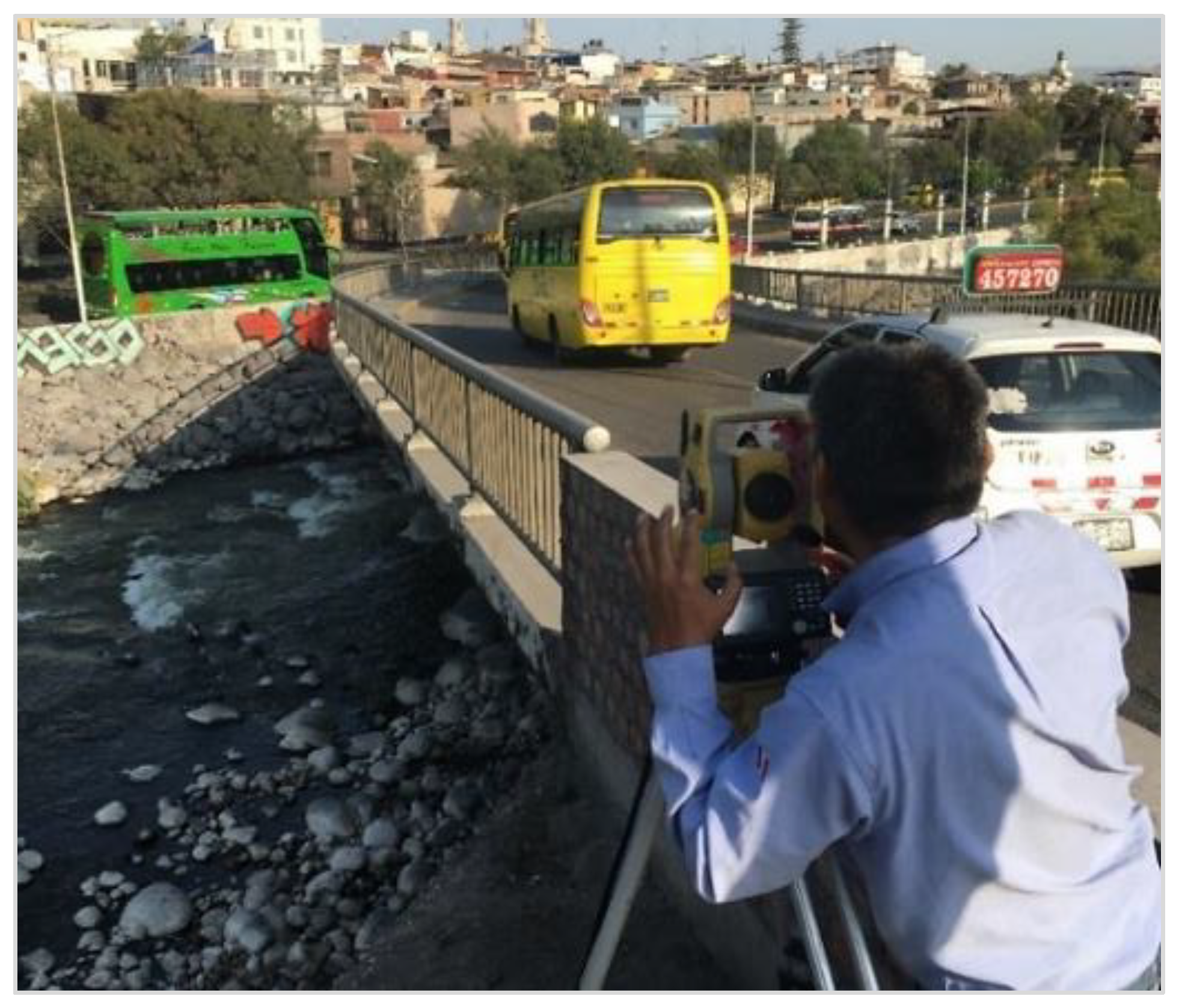
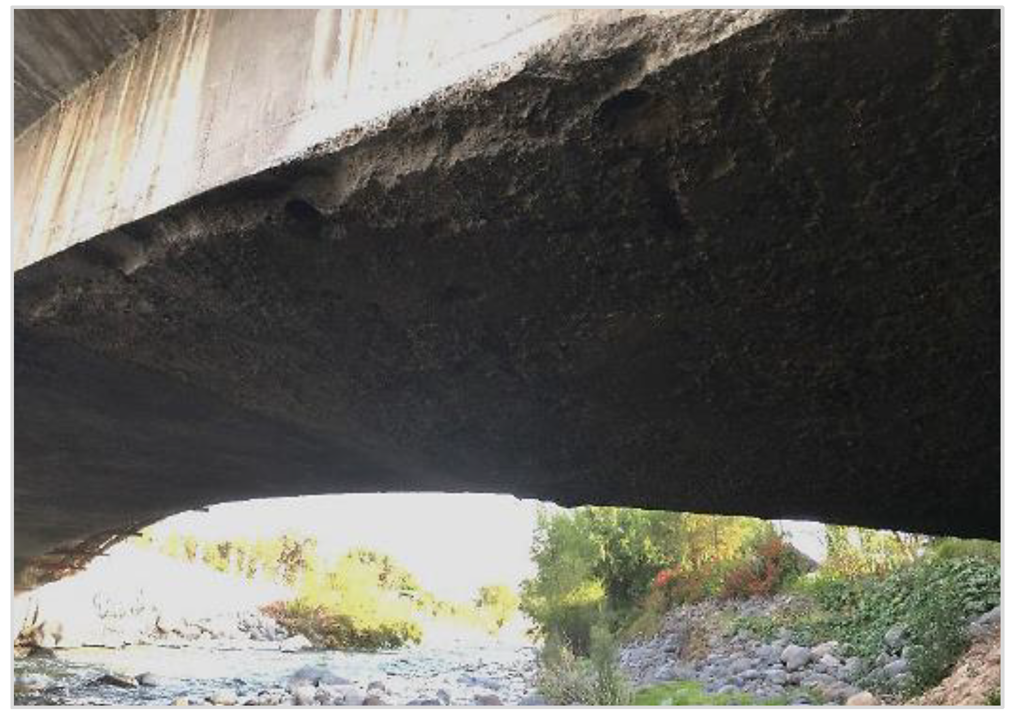
The information about the bridge was requested by the local city council. This included the design technical file, the location, architecture, and the structural plans of the bridge. However, not all of the information was available, as the design technical file and other documents had been lost. Thus, it became necessary to carry out a survey of the bridge and the riverbed to complement the insufficient information. Figure 1 shows a photograph of the survey carried out as seen from the highest part of the bridge, in the flow direction, from upstream to downstream. Additionally, a visual inspection was undertaken which revealed the erosion at the bottom of the bridge deck due to past flow impacts (Figure 2), and enabled information to be collected about the land use to get Manning’s roughness coefficient along the channel [21]; a key data set for the vulnerability analysis.

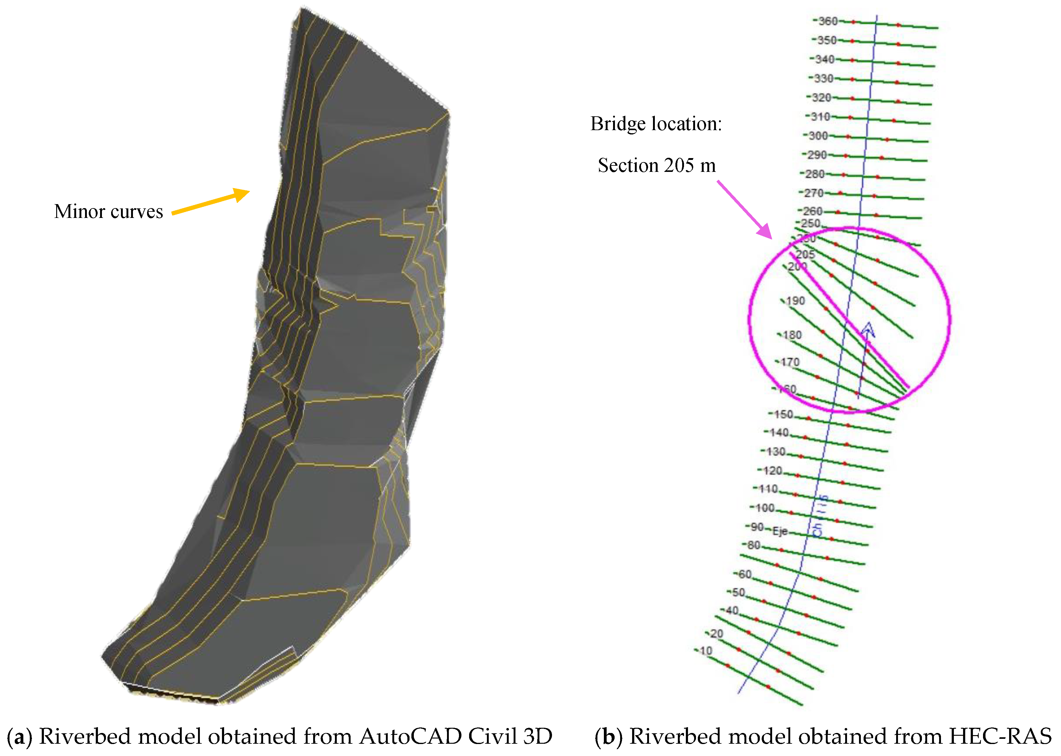
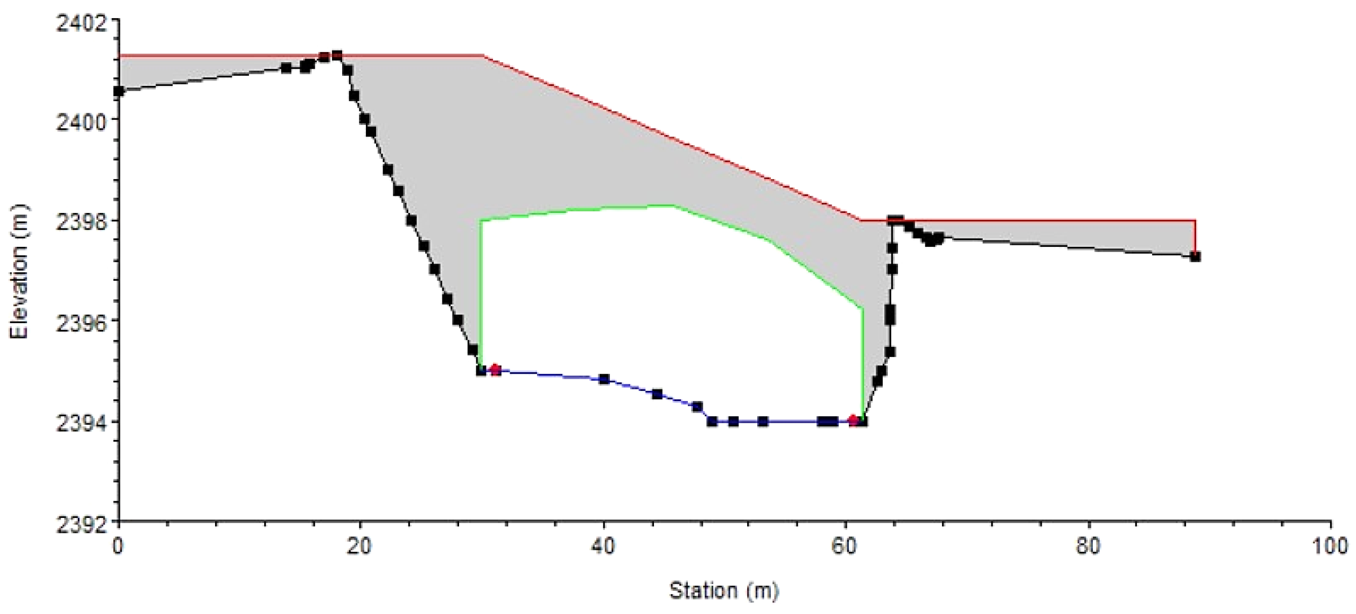
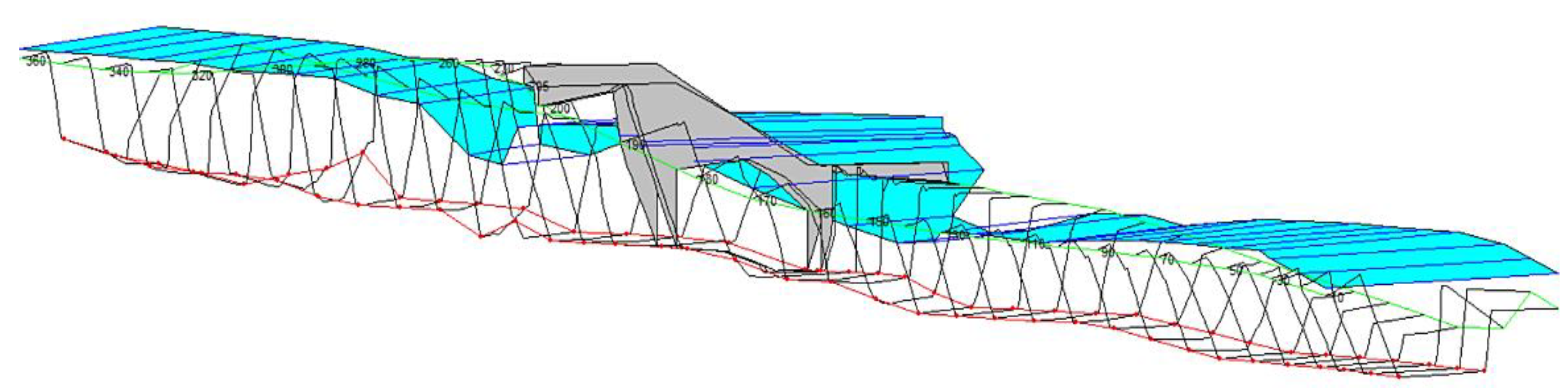
The software used to process the surveying information was AutoCAD Civil 3D. The contour lines (major curves every 5 m and minor curves every meter) were obtained, which led to a contour map. The variations, both longitudinal and transversal, of the Chili riverbed along 360 m were modelled in the software as well; the code [41] required a minimum of 150 m upstream and 150 m downstream. Once this process was finished, the geometry was imported from AutoCAD Civil 3D to HEC-RAS. This included the alignment, the flow direction, the cross sections every 10 m, the boundaries of the river, and the main axis. Figure 3 shows the riverbed models; the minor curves, the 36 cross sections and the bridge location in section 205 m (section 210 m was changed to section 205 m so that the bridge could be correctly located and aligned in the model). Figure 4 shows the cross section of the bridge in the channel from a downstream view. Consequently, the geometry of the bridge and the riverbed, which represent critical parameters for the study [21], were obtained. The modelling of the bridge is detailed in the hydraulic study.

2.2. Soil Mechanics Study

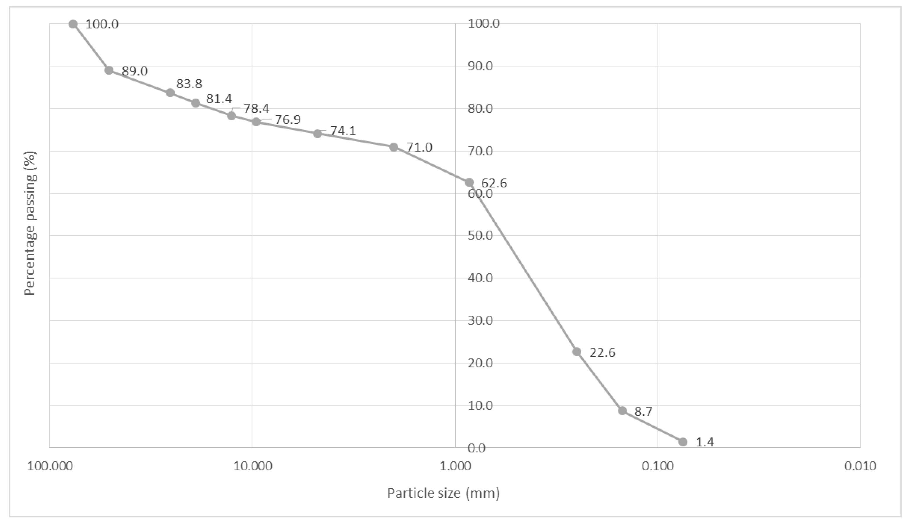
A fundamental parameter for the scouring analysis is the soil, since this phenomenon occurs where the bridge was founded; likewise, many of the equations for calculating general and local scour that will be discussed afterwards require data concerning the soil. Therefore, a test pit was made in the riverbed and 4 kg of soil were extracted; the soil samples were transferred to the laboratory in hermetically sealed bags. The tests were carried out to determine the following properties of the soil: particle size distribution, moisture content and specific weight.

The particle size analysis resulted in obtaining the deciles of the soil based on the distribution curve. Sieves of 2″, 1 ½″, 1″, ¾″, ½″, 3/8″ (inches, Imperial units used), and mesh no. 4, 10, 20, 60, 100, 200 were used (Figure 5). Similarly, after a laboratory analysis, the other two soil properties were obtained. The moisture content was 27.5% and the specific weight was 2.65 g/cm³. These two properties, along with the parameters obtained from the particle size distribution curve, concluded the direct collection of data from the soil and the bridge, and were ready to be used as inputs in the next stages of the vulnerability analysis.

3. Results

3.1. Hydrological Statistic and Scenarios Proposition

The Bajo Grau Bridge is located in the Medium Quilca-Vitor-Chili Hydrographic Unit, before the confluence with the Tingo Grande River [42]. This sector is regulated by the Aguada Blanca Dam and is reinforced upstream by the Charcani hydro-power station, and has hydrometric data due to the “Water Movement Chili System” [43]. Discharges have been monitored there since 1960, which allows for a statistical analysis to estimate the flow rates according to the risk and the return period (T) of the structure. A thorough hydrological study was necessary to predict the behaviour of the river following the recommendations given by the Peruvian code [44]. Extreme value analysis plays a major role in this regard, because random variables describing flows are essential to predict design values in engineering projects [45]. Even though there are no codes to analyse the hydrological vulnerability, the study of extreme values related to floods follows the same procedure, as the behaviour of the river is independent of the behaviour of the bridge.

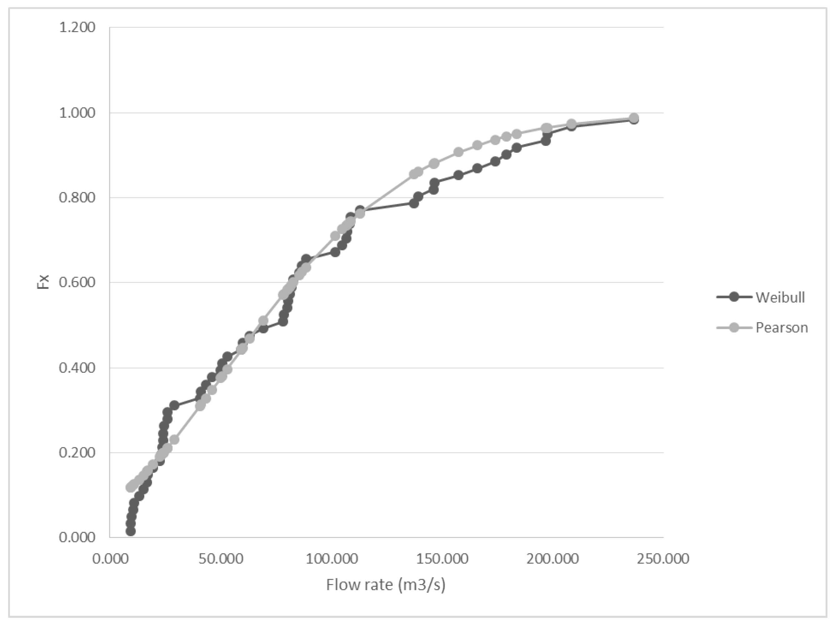
Consequently, the series of maximum annual flows was obtained, a graphic consistency analysis was carried out, and then the probability frequency analysis was conducted using four empirical and four theoretical distribution functions [44,46]. The Kolmogorov–Smirnov goodness of fit test, which has proved to be valuable when analysing hydrological data [45,47], enabled the selection of the best distribution by comparing the test statistics, D with d between all 16 possible combinations (

Table 1. Kolmogorov–Smirnov goodness of fit test combination results.

Empirical Model	Theoretical Model	Max Delta (D)	Tabular Delta (d)
California	Normal	0.121	0.176
	Log Normal	0.142
	Gumbel	0.111
	Pearson III	0.118
Weibull	Normal	0.110
	Log Normal	0.133
	Gumbel	0.122
	Pearson III	0.101
Gringorten	Normal	0.112
	Log Normal	0.133
	Gumbel	0.119
	Pearson III	0.108
Blom	Normal	0.111
	Log Normal	0.133
	Gumbel	0.120
	Pearson III	0.107

where D is the maximum absolute value of the difference D between the observed/empirical probability distribution function and the theoretical/estimated one, and d is the tabular value in the function of the sample size and the level of significance.

).

According to the analysis, the Pearson III distribution was the one that best fitted the hydrological data, as its D was lower than d and it was the lowest of all the other results. Figure 6 shows the Kolmogorov–Smirnov goodness of fit test with the empirical and the theoretical models.

The magnitude of an extreme hydrological event can be represented as the mean plus the product of the standard deviation and the frequency factor; these parameters are functions of the return period (T) and the type of probability distribution to be used in the analysis [44,48], in this case the Pearson III model. The flow rate prediction is based on the establishment of different scenarios that consider the bridge’s service life [41], the return period, an admissible risk to scouring and the extraordinary maximum water level [44]. Similarly, an additional scenario (scenario 6) was considered with Q = 500 m³/s, which is the design flow rate of the spillway [43] (see

Table 2. Flow rates based on each scenario.

Scenario	T (Years)	Q (m3/s)
1	100	251.74
2	200	276.45
3	400	325.87
4	500	350.57
5	1000	474.11
6	-	500.00

).

3.2. Hydraulic Aspects

Having concluded the hydrological study by obtaining the flow rates based on the six proposed scenarios for the Chili river basin, it was possible to advance to the next stage to determine the hydrological vulnerability of the bridge through hydraulic modelling. By doing this, two important outputs were obtained: the flow properties to determine the scouring in the substructure of the bridge, and the profile of the free surface of the flow along the channel to determine the flood-driven vulnerabilities.

For each flow condition, the elements of geometric description such as number of cross-sections, spacing, location and structural details are fundamental to achieving an optimal model [21]. As was previously mentioned, an essential input to the modelling was the topographic data of the channel obtained from the surveying. This parameter, along with the geometric configuration of the bridge, was exported to HEC-RAS. The bridge modelling in HEC-RAS enables the analysis of the bridge hydraulics by defining the deck and abutments as separate items [49], and the overall model enables the delineation of the areas vulnerable to floods at different discharge values [20]. The calculations are based on HEC-RAS equations for one-dimensional steady gradually varied flow, such as Energy equation [49] (Equation (1)):

$$z_2+\frac{P_2}{\gamma }+{\alpha }_2\frac{V_2^2}{2g}=z_1+\frac{P_1}{\gamma }+{\alpha }_1\frac{V_1^2}{2g}+E$$

(1)

where $z_1$ and $z_2$ are the elevations of the main channel inverts, $\frac{P_1}{\gamma }$ and $\frac{P_2}{\gamma }$ are the depths of water at cross sections, $V_1$ and $V_2$ are the average velocities, ${\alpha }_1$ and ${\alpha }_2$ are the velocities weighting coefficients, $g$ is the gravitational acceleration, and E is the energy head loss.

Consequently, the hydraulic simulation in the software was possible after providing the input data necessary for the analysis that the software required: flow rates, parameters of roughness obtained by Cowan’s method [50,51], cross section contraction and expansion coefficients, and slope and bridge dimensions. The results of the hydraulic simulation for the six scenarios at cross section 205 m are shown in

Table 3. Hydraulic simulation results at the bridge cross section.

Scenario	Return Period	Flow Rate (m3/s)	Min. Elevation (m)	Normal Flow Depth Elevation (m)	Critical Flow Depth Elevation (m)	Velocity (m/s)	Flow Area (m2)	Water Mirror (m)	Froude Number
1	100	251.74	2393.99	2397.49	2396.30	2.47	112.31	52.22	0.46
2	200	276.45	2393.99	2397.72	2396.41	2.50	125.64	65.14	0.45
3	400	325.87	2393.99	2398.16	2396.62	2.54	155.35	68.23	0.43
4	500	350.57	2393.99	2398.38	2396.72	2.52	170.14	68.67	0.41
5	1000	474.11	2393.99	2399.39	2397.19	2.47	240.67	70.09	0.36
6	1104	500.00	2393.99	2399.71	2397.29	2.39	263.19	70.37	0.34

.

Accordingly, the model shown in Figure 7 represents the simulation of the most critical scenario, which has a flow rate of Q = 500 m³/s and a flow area of 263.19 m² in the bridge section. As it can be seen, the water impacts the deck of the bridge, generating major flooding; the consequences are analysed in the vulnerability analysis.

Complying with the Peruvian regulations is an important aspect to consider when determining the hydrological vulnerability of the bridge. In this regard, the EMWL (Extraordinary Maximum Water Level) is a fundamental parameter to analyse.

Table 4. Results of the Extraordinary Maximum Water Level analysis.

Scenario	T (Years)	Inferior Deck Height (m)	Real EMWL Height (m)	Code EMWL Height (m)	Heights Difference (m)	Result
1	100	2396.24	2397.32	2394.24	3.08	Failure
2	200	2396.24	2397.51	2394.24	3.27	Failure
3	400	2396.24	2397.87	2394.24	3.63	Failure
4	500	2396.24	2398.02	2394.24	3.78	Failure
5	1000	2396.24	2399.00	2394.24	4.76	Failure
6	-	2396.24	2399.71	2394.24	5.47	Failure

presents the comparison between the deck height according to the code and the flow height after the simulations for each scenario. Every scenario fails to meet the Peruvian code design requirements, since the difference in dimensions between the deck and the EMWL exceeds the minimum difference of two meters.

3.3. Scouring Study

The beginning of the movement of a particle due to the action of the current occurs when the forces promoting its movement overcomes the stabilizing forces [52]. Some equations are based on this movement velocity, hence the importance of its calculation. Many widely used riverbed load sediment-transport models are based on the concept that sediment transport either begins at, or can be scaled by, a constant value of the non-dimensional bed-shear stress or the critical Shields stress [53]. The expressions used in this research are derived from an analysis of the critical velocity, as they incorporate this consideration in their formulas.

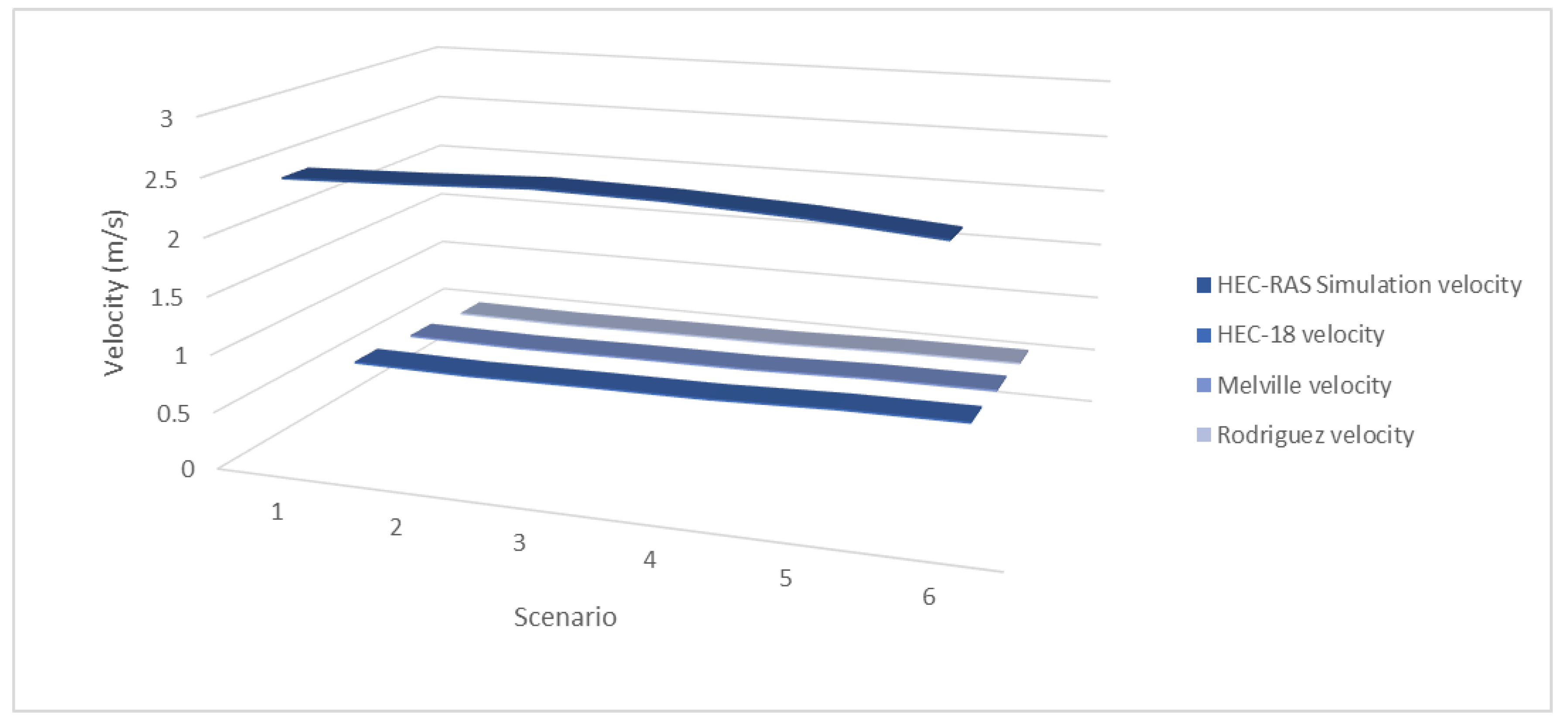
The erosive velocity is the parameter used to determine if the scour occurs in a live bed or clear water. A large number of the equations are based on this scour classification; therefore, it is necessary to determine it. It should be noted that scour depths in a live riverbed may be limited if there is an appreciable number of large particles at the bottom of the channel, in which case it is advisable to also use scour equations in clear water and choose a representative depth. As mentioned: (a) Clear water scour occurs when the erosive velocity is greater than the average velocity, V < V_e; and (b) Live bed scour occurs when the erosive velocity is less than the average velocity, V > V_e. Three methods were used to characterize the erosive velocity (Equations (2)–(4)); the comparison for the three calculation methods for D50 is presented in Figure 8. The scouring type is live bed.

Melville and Coleman [54]:

$$Ve=5.67y^{\frac{1}{6}}d{50}^{\frac{1}{3}}$$

(2)

Rodríguez Díaz [52]:

$$Ve=\frac{1}{n}{R}^{\frac{1}{6}}{\left(0.06\left(\gamma s-1\right)dm\right)}^{\frac{1}{2}}$$

(3)

Richardson and Davis [55], HEC-18:

$$Ve=Ku y^{\frac{1}{6}}d{50}^{\frac{1}{3}}$$

(4)

where $y$ is the flow depth, d50 is decile 50 of the particle size distribution curve, $n$ is the Manning roughness coefficient, $R$ is the hydraulic radius, γs is the specific gravity of the riverbed material, dm is the mean diameter of the riverbed particles, and $Ku$ is the coefficient based on the Shields parameter.

There are four kinds of scouring that can be determined: general, local, transversal and in curves [44]. The Bajo Grau Bridge stands in a straight section of the river, which is why the calculation of the scouring in curves was discarded from the analysis; however, the other three analyses were carried out. Furthermore, as the bridge does not have pillars, the local scouring analysis focuses on the bridge abutments.

As for the general scouring, the method by Lischtvan and Lebediev [56] was used (Equation (5)), as it has proved to be valuable for the calculation of this kind of scouring [57,58]. Moreover, this method incorporates the effect of contraction, which is why a further analysis of that type of scouring was not necessary.

$$Hs={\left(\frac{\alpha \ast H{o}^{\frac{5}{3}}}{0.68\ast \beta \ast d{m}^{0.28}}\right)}^{\frac{1}{1+z}}$$

(5)

where $Hs$ is the flow depth measured from the water surface to the eroded bottom; $Ho$ is the initial flow depth; $\alpha =\frac{S^{1/2}}{n}$ is the coefficient that depends on the roughness and energy gradient (S); $\beta =0.0973logT+0.79$ is the coefficient that depends on the return period of the flow rate; and $z=-0.0089lo{g}^{2}dm-0.041logdm+0.395$ is the coefficient that depends on the mean diameter of the riverbed particles.

As for the local scouring calculation in the abutments of the bridge, this was carried out using the comparison of three different methods (the Field method, and Equations (6) and (7)), where the most critical scouring for both abutments was obtained by the Froehlich [59] method.

Field 3-parameter method [60]:

$$\frac{DsM}{y},\frac{bM}{y},Fr\sqrt{M}$$

where $Ds=ds+y$ is the equilibrium scour depth, measured from the surface of the normal flow depth; ds is the local scour depth, measured from riverbed level; $M=\frac{B\prime }{B}$ is the aperture ratio; $B$ is the average width of the top of the upstream channel; B^′ is the width of the bridge aperture at a depth of y/2 below the normal flow surface; and $Fr$ is the Froude number.

Liu, et al. [61]:

$$\frac{Ds}{y}=2.15{(\frac{a}{Yo})}^{0.4}\ast F{r}^{0.33}$$

(6)

where $a$ is the width of the abutment or vertical body.

Froehlich [59]:

$$\frac{ds}{y}=2.27\ast K1\ast K2\ast {\left(\frac{b}{y}\right)}^{0.43}F{r}^{0.61}+1$$

(7)

where $K1$ is the correction factor based in the abutment shape, $K2$ is the correction factor based in the angle of impact of the flow against the abutment, and $b$ is the normal projection to the abutment, measured at the riverbed level.

The sum of the scouring components allowed the total potential scouring to be determined. As the code indicates [44], the three types were calculated for a return period of T = 500 years; therefore, the total potential scouring is also a function of that scenario. Under these considerations, the potential total scouring from a downstream perspective was 8.22 m in the left abutment and 7.32 in the right abutment.

4. Hydrological Vulnerability Assessment

The procedure used to determine the hydrological vulnerability of the bridge is based on the literature review and the previous bridge analysis. First, the types of vulnerabilities to be analysed were defined: Environmental Vulnerability (EV) and Physical Vulnerability (PV). Following this, different criteria and assessment parameters were assigned to each type of vulnerability. The classification criteria were established as low, medium, high and very high. Based on these considerations, a hydrological vulnerability assessment matrix was generated (

Table 5. Hydrological vulnerability assessment matrix.

Variable	Low—1	Medium—2	High—3	Very high—4
Environmental Vulnerability (EV) Levels
Flow rates variability	Average levels	Levels slightly higher than the average	Levels higher than the average	Levels much higher than the average
Water quality and composition	Low pollution levels	Medium pollution levels	High pollution levels	Very high pollution levels
Physical Vulnerability (PV) Levels
Building material used	Concrete, steel or similar resilient materials in a good state	Concrete, steel, wood or similar materials in a regular state	Wood or adobe without structural reinforcements in a bad state	Adobe, reed and minor resistance materials in precarious state
Location: proximity to a populated centre	Far, >5 Km.	Moderately close, 1–5 km	Close, 0.2–1 km,	Very close, 0.2–0 km
Soil quality along the riverbed	Good conditions, without obstructions and/or variability	Regular conditions, without many obstructions and/or variability	Bad conditions, with obstructions and variability	Very bad conditions, with obstructions and great variability
Geometric characteristics—Bridge height	The height allows the water to flow without inconvenience. It has more than 2 m of variance between the water surface and the deck underside	The height allows the water to flow without inconvenience. It has less than 2 m of variance between the water surface and the deck underside	The height does not allow the water to flow normally. The water level reaches the deck	The height does not allow water to flow normally. The water level surpasses the deck
Erosion on the deck	The deck is not reached by the water flow	The deck is reached in the underside by the water flow, causing erosion	The deck is reached in a bigger area by the water flow, causing further erosion	The whole deck is reached by the water flow. It causes erosion in the upper section too
Protection against scouring	The abutments are protected against the flow	The abutments are moderately protected against the flow	The abutments are poorly protected against the flow	The abutments are unprotected against the flow
Overflow and flooding	The flow does not exceed the deck height and does not overflow	The flow reaches the deck height, but does not overflow	The flow reaches the deck height and overflows	The flow exceeds the deck height, causing overflow and flooding
Regulations compliance	Strictly compliance of the code	Moderately compliance of the code	Low compliance of the code	Without compliance of the code

).

Considering the results of the bridge analysis, the matrix was used to give a score to each criterion, making it possible to obtain a value for each type of vulnerability. It should be noted that some criteria had higher weightings than others, because they represent a greater vulnerability for the bridge. Furthermore, considering that the PV is directly related to the structure and its possible failure, it was assigned a higher weighting than EV. Under these considerations, the hydrological vulnerability of the bridge was calculated.

5. Environmental Vulnerability (EV)

5.1. Flow Rate Variability

Through a graphic consistency analysis, it was determined that the flows of the Chili River have been increasing considerably (taking into account the data since 1960). Climate change and the lack of maintenance of the dams in the basin are the reasons for this situation. Therefore, a score of 3 was assigned to this criterion.

5.2. Water Quality and Composition

This criterion is based on two main factors. The first one relates to the fact that if the water carries solid waste such as logs (due to pollution), the erosion on the bridge would be greater than a normal (not polluted) flow. The second one is related to the impact on the environment itself; in case of flooding, the negative effect on the neighbour ecosystem would be greater as well. As the Chili River has a high degree of pollution [62,63], this evaluation parameter has a value of 3.

Therefore, the $EV$ is determined as high:

$$EV=0.5 \left(3\right)+0.5 \left(3\right)$$

$$EV=3.0$$

6. Physical Vulnerability (PV)

6.1. Building Material Used

The bridge is made of reinforced concrete, a resistant material. However, as evidenced in the visits to the bridge, it shows erosion due to the impact of the flow. That is why its vulnerability was determined as medium (rating of 2).

6.2. Location

The bridge connects two important roads, the avenues La Marina and El Ejercito. These are located in the centre of the city, a location that produces a greater vulnerability (rating of 4), not only because of the high traffic of vehicles; but also due to the impact that this could have if the scenario for a return period of 500 years is reached; that is, the flooding of La Marina Avenue and the damage to the buildings located along it.

6.3. Soil Quality

As a result of the inspection 150 m upstream and 150 m downstream of the bridge, and the soil study, it was determined that the riverbed presents a regular condition, therefore it is given a rating of 2.

6.4. Geometric Characteristics of the Bridge

As presented in the models, the flow reaches the superstructure for every scenario. The deck should increase its height with respect to the Extraordinary Maximum Water Level. This variation in height also implies an increase in the length of the deck, as well as a change in its slope and possibly new features in the substructure, such as the placement of pillars. Hence, it is given a rating of 3.

6.5. Erosion on the Deck

Through the inspection carried out on the bridge, it was observed that there is erosion in the lower part of the deck derived from the impact of the river flow. Similarly, the results for all critical scenarios translates into an impact on the deck; this supposes an incremental erosive process in such a way that it increases the fragility of the bridge. Thus, the vulnerability is high (a rating of 3).

6.6. Protection against Scouring

Since there were no plans or technical specifications for the bridge, a study of the foundation needed to be carried out to determine if the calculated scouring exceeds the depth of the abutments. Such an evaluation is out of the scope of this research, which is why this parameter was estimated according to the protection of the bridge abutments, which are moderately protected against the flow (a rating of 2).

6.7. Overflow and Flooding

It was observed that for a return period of 500 years, the water flow exceeds the cross section of the bridge, as well as the sections upstream, due to the fact that, among other factors, there is a contraction in that area. The result of the poor location of the bridge, as well as its geometry, is that it produces a flood on La Marina Avenue. Hence, this criterion was estimated as high (a rating of 4).

6.8. Regulations Compliance

Bridges should provide security. Although the bridge does comply with certain regulations, the modelling carried out reveals the non-compliance with certain regulatory parameters, such as the height of the bridge. Therefore, a rating of 2 was assigned to this criterion.

Therefore, the PV is determined as high:

$$PV=0.1\ast \left(2\right)+0.1\ast \left(4\right)+0.1\ast \left(2\right)+0.2\ast \left(3\right)+0.1\ast \left(3\right)+0.1\ast \left(2\right)+0.2\ast \left(4\right)+0.1\ast \left(2\right)$$

$$PV=2.9$$

7. Hydrological Vulnerability (HV)

Finally, using the two evaluation parameters established for the $EV$ and the eight parameters for the $PV$, and following the same classification criteria for each variable of the matrix, the vulnerability of the bridge, being 2.9, was determined as high:

$$HV=0.20EV+0.80PV$$

$$HV=0.20\left(3.0\right)+0.80\left(2.9\right)$$

$$\mathit{H}\mathit{V}=\mathbf{2.9}$$

8. Discussion

The bridge hydrological assessment methodology was validated through a case study; however, its implementation process in public bodies in charge of managing bridges is the subject of further analysis. The proposed methodology, which complies with Peruvian regulatory requirements, could be adapted to bridges with similar characteristics as long as there is an investment directed at risk management. The three levels of the Peruvian government have sufficient financial resources to implement this type of process; however, there is a low spending capacity, particularly at the local government level [64,65]. This has been a trend in recent years, so much so that the long-term infrastructure gap in Peru is 110 billion dollars [66]. In order to progressively close this gap and invest in the whole life cycle of infrastructure systems, proposals are needed to solve the issues that pertain to the population, ensuring their safety and avoiding large economic losses due to failures or collapses of essential infrastructure systems such as bridges.

On the other hand, it should be noted that Peruvian regulations include outdated design parameters. Implementing technological and innovative processes has become more than an option, a necessity. Peruvian standards are just taking the first steps to implement more efficient management systems such as BIM (Building Information Modelling), which also generate greater transparency in the use of resources to plan, design, operate, maintain and even dispose of infrastructure. Consequently, the methodology to evaluate bridges could utilise up to date models for greater precision in the calculations, such as 3D models and CFD (Computational Fluid Dynamics) [67,68]. Furthermore, a great complement to the methodology would be efficient alternatives to manage the risks derived from the vulnerability analysis; for example, sensors could be placed in the infrastructure under SHM (Structural Health Monitoring) on priority interventions [69,70].

9. Conclusions

The proposed methodology to calculate the hydrological vulnerability of bridges that cross rivers is based on ten different criteria grouped into two types of vulnerabilities that are part of the hydrological vulnerability. The number of criteria that can be considered, as well as the types of vulnerabilities, are not limited, i.e., more assessment parameters can be proposed in the determination of the characteristics of the bridge. Consequently, the hydrological vulnerability assessment matrix can be adapted for its use in other bridges.

Regarding the case study, the Bajo Grau Bridge presents a high hydrological vulnerability. Several factors enabled the assessment of the bridge: the field exploration, the soil study, the topographic surveying, the hydrological statistics based on the annual maximum flow rates of the river, the hydraulic modelling in HEC-RAS, and the scouring study. The study shows that the bridge represents a danger for passers-by, especially in the rainy season when the flow of the Chili River in the city increases. That is why it is recommended to complement this hydrological analysis with a seismic and structural one; so that, based on this, alternatives for optimizing the bridge are proposed. In case of a reconstruction, the height of the bridge should be 4 m higher than it is currently, since, as evidenced in the modelling, the flow would impact the bridge deck in the most critical scenarios, and its current height does not meet current regulatory requirements. Moreover, the foundation depth for the abutments should be 8.5 m.

This research contributes to closing the knowledge gap regarding the analysis of important vulnerable structures such as bridges by proposing a novel methodology that can be transferred to other structures that can have a positive impact as long as it is properly implemented.

References

- Proske, D. Comparison of the collapse frequency and the probability of failure of bridges. Proc. Inst. Civ. Eng.-Bridge Eng. 2019, 172, 27–40. [Google Scholar] [CrossRef]
- Shirhole, A.; Holt, R. Planning for a comprehensive bridge safety program. Transp. Res. Rec. 1991, 1290, 39–50. [Google Scholar]
- Wardhana, K.; Hadipriono, F.C. Analysis of recent bridge failures in the United States. J. Perform. Constr. Facil. 2003, 17, 144–150. [Google Scholar] [CrossRef] [Green Version]
- Mondoro, A.; Frangopol, D.M.; Liu, L. Bridge Adaptation and Management under Climate Change Uncertainties: A Review. Nat. Hazards Rev. 2018, 19, 04017023. [Google Scholar] [CrossRef]
- Smith, D. Bridge failures. Proc. Inst. Civ. Eng. 1976, 60, 367–382. [Google Scholar] [CrossRef]
- Pregnolato, M.; Winter, A.O.; Mascarenas, D.; Sen, A.D.; Bates, P.; Motley, M.R. Assessing flooding impact to riverine bridges: An integrated analysis. Nat. Hazards Earth Syst. Sci. Discuss. 2020, 2020, 1–18. [Google Scholar] [CrossRef]
- Bastidas-Arteaga, E.; Stewart, M.G. Damage risks and economic assessment of climate adaptation strategies for design of new concrete structures subject to chloride-induced corrosion. Struct. Saf. 2015, 52, 40–53. [Google Scholar] [CrossRef] [Green Version]
- Kosič, M.; Anžlin, A.; Bau’, V. Flood Vulnerability Study of a Roadway Bridge Subjected to Hydrodynamic Actions, Local Scour and Wood Debris Accumulation. Water 2023, 15, 129. [Google Scholar] [CrossRef]
- Rowan, E.; Evans, C.; Riley-Gilbert, M.; Hyman, R.; Kafalenos, R.; Beucler, B.; Rodehorst, B.; Choate, A.; Schultz, P. Assessing the Sensitivity of Transportation Assets to Extreme Weather Events and Climate Change. Transp. Res. Rec. 2013, 2326, 16–23. [Google Scholar] [CrossRef]
- La Republica. Cierran tres puentes ante posible desborde del río Chili en Arequipa. La Republica, 2019. [Google Scholar]
- Méndez, R. Cierran Puentes en Arequipa por Incremento del Caudal del río Chili. Andina. 2012. Available online: https://andina.pe/agencia/noticia-cierran-puentes-arequipa-incremento-del-caudal-del-rio-chili-399604.aspx (accessed on 11 January 2023).
- Riva, R. Cierran Tres Puentes Ante Posible Desborde del río Chili en Arequipa. RPP. 2011. Available online: https://rpp.pe/peru/actualidad/cierran-tres-puentes-ante-posible-desborde-del-rio-chili-en-arequipa-noticia-339102 (accessed on 11 January 2023).
- Gharbi, M.; Soualmia, A.; Dartus, D.; Masbernat, L. Comparison of 1D and 2D hydraulic models for floods simulation on the Medjerda Riverin Tunisia. J. Mater. Environ. Sci. 2016, 7, 3017–3026. Available online: https://scholar.google.com/scholar_lookup?hl=en&volume=7%288%29&publication_year=2016&pages=3017-3026&author=M.+Gharbi&author=A.+Soualmia&author=D.+Dartus&author=L.+Masbernat&title=Comparison+of+1D+and+2D+hydraulic+models+for+floods+simulation+on+the+medjerda+river+in+tunisia (accessed on 11 January 2023).
- Anees, M.T.; Abdullah, K.; Nawawi, M.N.M.; Ab Rahman, N.N.; Piah, A.R.; Zakaria, N.A.; Syakir, M.I.; Omar, A.K. Numerical modeling techniques for flood analysis. J. Afr. Earth Sci. 2016, 124, 478–486. [Google Scholar] [CrossRef]
- Papaioannou, G.; Loukas, A.; Vasiliades, L.; Aronica, G.T. Flood inundation mapping sensitivity to riverine spatial resolution and modelling approach. Nat. Hazards 2016, 83, 117–132. [Google Scholar] [CrossRef]
- Timbadiya, P.V.; Patel, P.L.; Porey, P.D. HEC-RAS based hydrodynamic model in prediction of stages of lower Tapi River. ISH J. Hydraul. Eng. 2011, 17, 110–117. [Google Scholar] [CrossRef]
- Popescu, C.; Bărbulescu, A. Floods Simulation on the Vedea River (Romania) Using Hydraulic Modeling and GIS Software: A Case Study. Water 2023, 15, 483. [Google Scholar] [CrossRef]
- Merkuryeva, G.; Merkuryev, Y.; Sokolov, B.V.; Potryasaev, S.; Zelentsov, V.A.; Lektauers, A. Advanced river flood monitoring, modelling and forecasting. J. Comput. Sci. 2015, 10, 77–85. [Google Scholar] [CrossRef]
- Ghimire, E.; Sharma, S.; Lamichhane, N. Evaluation of one-dimensional and two-dimensional HEC-RAS models to predict flood travel time and inundation area for flood warning system. ISH J. Hydraul. Eng. 2022, 28, 110–126. [Google Scholar] [CrossRef]
- Ahmad, B.; Kaleem, M.S.; Butt, M.J.; Dahri, Z.H. Hydrological modelling and flood hazard mapping of Nullah Lai. Proc. Pak. Acad. Sci. 2010, 47, 215–226. [Google Scholar]
- Cook, A.; Merwade, V. Effect of topographic data, geometric configuration and modeling approach on flood inundation mapping. J. Hydrol. 2009, 377, 131–142. [Google Scholar] [CrossRef]
- Deng, L.; Cai, C.S. Bridge Scour: Prediction, Modeling, Monitoring, and Countermeasures—Review. Pract. Period. Struct. Des. Constr. 2010, 15, 125–134. [Google Scholar] [CrossRef] [Green Version]
- Garg, V.; Setia, B.; Singh, V.; Kumar, A. Scour protection around bridge pier and two-piers-in-tandem arrangement. ISH J. Hydraul. Eng. 2022, 28, 251–263. [Google Scholar] [CrossRef]
- Khalid, M.; Muzzammil, M.; Alam, J. A reliability-based assessment of live bed scour at bridge piers. ISH J. Hydraul. Eng. 2021, 27, 105–112. [Google Scholar] [CrossRef]
- Bathrellos, G.D.; Karymbalis, E.; Skilodimou, H.D.; Gaki-Papanastassiou, K.; Baltas, E.A. Urban flood hazard assessment in the basin of Athens Metropolitan city, Greece. Environ. Earth Sci. 2016, 75, 319. [Google Scholar] [CrossRef]
- Mani, P.; Chatterjee, C.; Kumar, R. Flood hazard assessment with multiparameter approach derived from coupled 1D and 2D hydrodynamic flow model. Nat. Hazards 2014, 70, 1553–1574. [Google Scholar] [CrossRef]
- Akay, H.; Baduna Koçyiğit, M. Hydrologic assessment approach for river bridges in western Black Sea basin, Turkey. J. Perform. Constr. Facil. 2020, 34, 04019090. [Google Scholar] [CrossRef]
- Liu, W.-C.; Hsieh, T.-H.; Liu, H.-M. Flood Risk Assessment in Urban Areas of Southern Taiwan. Sustainability 2021, 13, 3180. [Google Scholar] [CrossRef]
- Geng, Y.; Zheng, X.; Wang, Z.; Wang, Z. Flood risk assessment in Quzhou City (China) using a coupled hydrodynamic model and fuzzy comprehensive evaluation (FCE). Nat. Hazards 2020, 100, 133–149. [Google Scholar] [CrossRef] [Green Version]
- Glas, H.; De Maeyer, P.; Merisier, S.; Deruyter, G. Development of a low-cost methodology for data acquisition and flood risk assessment in the floodplain of the river Moustiques in Haiti. J. Flood Risk Manag. 2020, 13, e12608. [Google Scholar] [CrossRef]
- Garrote, J.; Díez-Herrero, A.; Escudero, C.; García, I. A Framework Proposal for Regional-Scale Flood-Risk Assessment of Cultural Heritage Sites and Application to the Castile and León Region (Central Spain). Water 2020, 12, 329. [Google Scholar] [CrossRef] [Green Version]
- Mitoulis, S.A.; Argyroudis, S.A.; Loli, M.; Imam, B. Restoration models for quantifying flood resilience of bridges. Eng. Struct. 2021, 238, 112180. [Google Scholar] [CrossRef]
- Chandrasekaran, S.; Banerjee, S. Retrofit Optimization for Resilience Enhancement of Bridges under Multihazard Scenario. J. Struct. Eng. 2016, 142, C4015012. [Google Scholar] [CrossRef]
- Dong, Y.; Frangopol, D.M. Probabilistic Time-Dependent Multihazard Life-Cycle Assessment and Resilience of Bridges Considering Climate Change. J. Perform. Constr. Facil. 2016, 30, 04016034. [Google Scholar] [CrossRef]
- Patel, D.A.; Lad, V.H.; Chauhan, K.A.; Patel, K.A. Development of Bridge Resilience Index Using Multicriteria Decision-Making Techniques. J. Bridge Eng. 2020, 25, 04020090. [Google Scholar] [CrossRef]
- Lad, V.H.; Patel, D.A.; Chauhan, K.A.; Patel, K.A. Development of Fuzzy System Dynamics Model to Forecast Bridge Resilience. J. Bridge Eng. 2022, 27, 04022114. [Google Scholar] [CrossRef]
- Lad, V.; Patel, D.; Chauhan, K.; Patel, K. Development of causal loop diagram for bridge resilience. In Proceedings of the 37th Annual Association of Research in Construction Management Conference, Glasgow, UK, 6–7 September 2021; pp. 137–146. [Google Scholar]
- Concha, C.J.; Miranda, A.G. Análisis del Riesgo de Inundación de la Cuencia del Río Chili en el Tramo de Chilina a Uchumayo-Arequipa; Universidad Católica de Santa María: Arequipa, Peru, 2016. [Google Scholar]
- Paredes Pinto, J.C. Gestión de Riesgos Bajo el Enfoque del PMI en Obras Viales Existentes–Caso: Puente Bajo Grau, Arequipa. Master’s Thesis, Universidad Católica de Santa María, Arequipa, Peru, 2019. [Google Scholar]
- INDECI. Manual Básico Para la Estimación de Riesgo/Basic Manual for Risk Estimation; Dirección Nacional de Prevención—Instituto Nacional de Defensa Civil: Lima, Peru, 2006. [Google Scholar]
- MTC in English: Ministry of Transport and Communications. Peruvian Code. Title in English: Bridge Manual. Lima, Peru. Available online: https://portal.mtc.gob.pe/transportes/caminos/normas_carreteras/documentos/manuales/MANUAL%20DE%20PUENTES%20PDF.pdf (accessed on 13 February 2023).
- ANA in English: Water National Authority. Peruvian Guideline. Title in English: Water Resources Management Plan of the Quica-Chili Basin. Available online: https://repositorio.ana.gob.pe/handle/20.500.12543/10 (accessed on 13 February 2023).
- AUTODEMA in English: Autonomous Authority of Majes. Peruvuan Guideline. Title English: Chili System Water Movement. Available online: https://www.autodema.gob.pe/movimiento-hidrico (accessed on 13 February 2023).
- MTC in English: Ministry of Transport and Communications. Peruvian Code. Title in English: Manual of Hidrology, Hydraulics and Drainage. Lima, Peru. Available online: http://transparencia.mtc.gob.pe/idm_docs/normas_legales/1_0_2950.pdf (accessed on 13 February 2023).
- Kottegoda, N.T.; Rosso, R. Statistics, Probability, and Reliability for Civil and Environmental Engineers; McGraw-Hill: New York, NY, USA, 1997. [Google Scholar]
- Chereque Morán, W. Hidrología: Para Estudiantes de Ingeniería Civil; Pontificia Universidad Católica del Perú: Lima, Peru, 1989. [Google Scholar]
- Aparicio Mijares, F.J. Fundamentos de Hidrología de Superficie; Limusa: Mexico City, Mexico, 1989. [Google Scholar]
- Te Chow, V.; Maidment, D.R.; Mays, L.W. Applied Hydrology; McGraw-Hill: New York, NY, USA, 1988. [Google Scholar]
- Brunner, G.W. HEC-RAS River Analysis System Version 4.1. 2010, US Army Corps of Engineers, Institute of Water Resources, Hydrologic Engineering Center (HEC). Available online: https://www.hec.usace.army.mil/software/hec-ras/documentation/HEC-RAS_4.1_Users_Manual.pdf (accessed on 14 February 2023).
- Cowan, W.L. Estimating hydraulic roughness coefficients. Agric. Eng. 1956, 37, 473–475. [Google Scholar]
- Marcus, W.A.; Roberts, K.; Harvey, L.; Tackman, G. An Evaluation of Methods for Estimating Manning’s n in Small Mountain Streams. Mt. Res. Dev. 1992, 12, 227. [Google Scholar] [CrossRef]
- Rodríguez Díaz, H.A. Hidráulica fluvial. Fundamentos y Aplicaciones. Socavación. Colombia. 2010. Available online: https://repositorio.escuelaing.edu.co/handle/001/1728?show=full (accessed on 14 February 2023).
- Lamb, M.P.; Dietrich, W.E.; Venditti, J.G. Is the critical Shields stress for incipient sediment motion dependent on channel-bed slope? J. Geophys. Res. 2008, 113, F02008. [Google Scholar] [CrossRef] [Green Version]
- Melville, B.W.; Coleman, S.E. Bridge Scour; Water Resources Publication: Highlands Ranch, CO, USA, 2000. [Google Scholar]
- Richardson, E.V.; Davis, S.R. Evaluating Scour at Bridges; Federal Highway Administration, Office of Bridge Technology: Washington, DC, USA, 2001. [Google Scholar]
- Lischtvan, L.; Lebediev, V. Gidrologia I Gidraulika v Mostovom Doroshnom, Straitielvie. Hydrology and Hydraulics in Bridge and Road Building; Gidrometeoizdat: Leningrad, USSR, 1959. [Google Scholar]
- Juarez, E.; Rico, A. Mecánica de suelos; Flujo de Agua en suelos. tomo III. Mexico. 1984. Available online: https://www.academia.edu/34972391/Mec%C3%A1nica_de_suelos_Tomo_III_Eulalio_Ju%C3%A1rez_Badillo_y_Alfonso_Rico_Rodr%C3%ADguez (accessed on 14 February 2023).
- Schreider, M.; Scacchi, G.; Franco, F.; Fuentes, R.; Moreno, C. Aplicación del método de Lischtvan y Lebediev al cálculo de la erosión general. Tecnol. Y Cienc. Del Agua 2001, 16, 15–26. [Google Scholar]
- Froehlich, D.C. Local scour at bridge abutments. In Proceedings of the 1989 National Conference on Hydraulic Engineering, New Orleans, LA, USA, 14–18 August 1989; pp. 13–18. [Google Scholar]
- Simons, D.; Lewis, G.; Field, W. Embankment protection at river constrictions. In Proceedings of the Colorado State University, Bridge Engineering Conference, Fort Collins, CO, USA, 1970. [Google Scholar]
- Liu, H.-K.; Chang, F.M.; Skinner, M.M. Effect of Bridge Constriction on Scour and Backwater; Colorado State University: Fort Collins, CO, USA, 1961; Available online: https://hdl.handle.net/10217/186161 (accessed on 14 February 2023).
- Salazar Pinto, B.; Cutipa Luque, J.; Ramírez Valverde, G.; Juyo Salazar, R.; Paredes Fuentes, J.; Villanueva Salas, J. Estudio de la contaminación por cromo (Cr) en el río chili y parque industrial de río seco (PIRS), Arequipa—Perú 2015–2016. Veritas 2017, 16, 43–46. [Google Scholar] [CrossRef]
- Dueñas Mejia, A.L.; Astoyauri Chipana, F.F. Problema de la Contaminación del río Chili Vulnera el Principio Constitucional de Protección de la Salud Arequipa 2021. Moquegua, Peru. 2022. Available online: https://hdl.handle.net/20.500.12819/1720 (accessed on 14 February 2023).
- Ministry of Economy and Finance. Economic Transparency—Expenditure Execution Consultation; Ministry of Economy and Finance, 2022. Available online: https://www.mef.gob.pe/es/?option=com_content&language=es-ES&Itemid=100944&lang=es-ES&view=article&id=504 (accessed on 13 February 2023).
- CGP. Effectiveness of Public Investment at the Regional and Local Levels during the Period 2009 to 2014 (EFECTIVIDAD de la inversión Pública a Nivel Regional y Local durante el Período 2009 al 2014). Lima, Peru. 2016. Available online: http://doc.contraloria.gob.pe/estudios-especiales/estudio/2016/Estudio_Inversion_Publica.pdf (accessed on 14 February 2023).
- Bonifaz, J.L.; Urrunaga, R.; Aguirre, J.; Quequezana, P.; Pastor, C.; Brichetti, J.P. Infrastructure Gap in Peru (Brecha de Infraestructura en el Perú); Inter-American Development Bank: Washington, DC, USA, 2019. [Google Scholar]
- Mignot, E.; Dewals, B. Hydraulic modelling of inland urban flooding: Recent advances. J. Hydrol. 2022, 609, 127763. [Google Scholar] [CrossRef]
- Rong, Y.; Zhang, T.; Zheng, Y.; Hu, C.; Peng, L.; Feng, P. Three-dimensional urban flood inundation simulation based on digital aerial photogrammetry. J. Hydrol. 2020, 584, 124308. [Google Scholar] [CrossRef]
- Seo, J.; Hu, J.W.; Lee, J. Summary review of structural health monitoring applications for highway bridges. J. Perform. Constr. Facil. 2016, 30, 04015072. [Google Scholar] [CrossRef]
- Prendergast, L.J.; Limongelli, M.P.; Ademovic, N.; Anžlin, A.; Gavin, K.; Zanini, M. Structural Health Monitoring for Performance Assessment of Bridges under Flooding and Seismic Actions. Struct. Eng. Int. 2018, 28, 296–307. [Google Scholar] [CrossRef] [Green Version]
Figure 1.
Surveying of the bridge.
Figure 2.
Erosion on the deck of the bridge.
Figure 3.
Riverbed models.
Figure 4.
Cross section of the bridge.
Figure 5.
Particle size distribution curve.
Figure 6.
Kolmogorov–Smirnov goodness of fit test.
Figure 7.
HEC-RAS hydraulic simulation for scenario 6, with a flow rate of Q = 500 m3/s.
Figure 8.
Erosive velocity methods comparison.