
Predictive Modelling of Reference Evapotranspiration Using Machine Learning Models Coupled with Grey Wolf Optimizer

1
Irrigation and Drainage Engineering Division, ICAR—Central Institute of Agricultural Engineering, Bhopal 462038, India
2
Outreach Program (ICAR-CIAE), ICAR—Indian Agricultural Research Institute, New Delhi 110012, India
3
Agricultural Mechanization Division, ICAR—Central Institute of Agricultural Engineering, Bhopal 462038, India
4
Faculty of Science, University of Technology Sydney, Sydney, NSW 2007, Australia
*
Authors to whom correspondence should be addressed.
Water 2023, 15(5), 856; https://doi.org/10.3390/w15050856
Submission received: 19 January 2023
/
Revised: 7 February 2023
/
Accepted: 20 February 2023
/
Published: 22 February 2023
(This article belongs to the Special Issue Application of Various Hydrological Modeling Techniques and Methods in River Basin Management)
Abstract
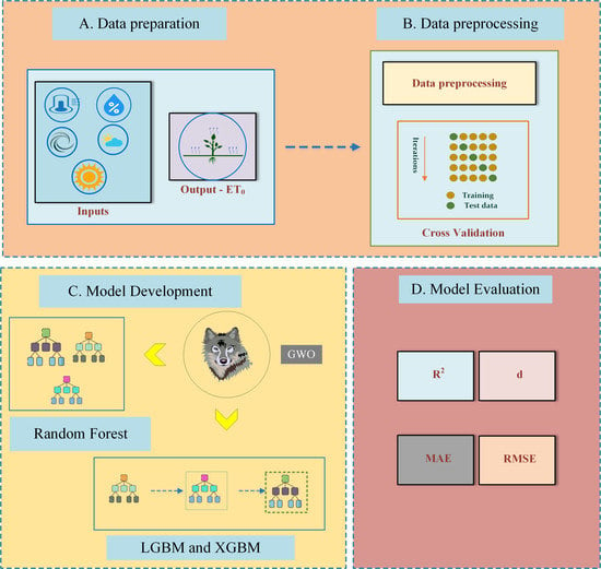
:Mismanagement of fresh water is a primary concern that negatively impacts agricultural productivity. Judicious use of water in agriculture is possible by estimating the optimal requirement. The present practice of estimating crop water requirements is using reference evapotranspiration (ET0) values, which is considered a standard method. Hence, predicting ET0 is vital in allocating and managing available resources. In this study, different machine learning (ML) algorithms, namely random forests (RF), extreme gradient boosting (XGB), and light gradient boosting (LGB), were optimized using the naturally inspired grey wolf optimizer (GWO) viz. GWORF, GWOXGB, and GWOLGB. The daily meteorological data of 10 locations falling under humid and sub-humid regions of India for different cross-validation stages were employed, using eighteen input scenarios. Besides, different empirical models were also compared with the ML models. The hybrid ML models were found superior in accurately predicting at all the stations than the conventional and empirical models. The reduction in the root mean square error (RMSE) from 0.919 to 0.812 mm/day in the humid region and 1.253 mm/day to 1.154 mm/day in the sub-humid region was seen in the least accurate model using the hyperparameter tuning. The RF models have improved their accuracies substantially using the GWO optimizer than LGB and XGB models.
1. Introduction
India is projected to be the World’s most populous country by 2023, surpassing China, which will have to feed about 1.66 billion people by 2050 [1]. Thus, the pressure on natural resources and food systems to produce more food would become a reality. Effective planning on water resource utilization should be the objective for water resource planners. The per capita availability of water is decreasing day by day due to the increase in population. According to the Ministry of Jal Shakti, Government of India, the average annual per capita water availability was 1816 cubic meters, 1545 cubic meters, and 1487 cubic meters for 2001, 2011, and 2021, respectively. It was estimated to further deteriorate to 1367 cubic meters by 2031.
Efficient water management in agriculture is required in developing nations, which are disadvantaged due to the lack of infrastructure and scientific advancements [2]. The need for crop water requirement-based irrigation practices in these nations is high to improve irrigation efficiency. Various methods and techniques are used to estimate the crop water requirement, of which the reference evapotranspiration (ET0) is a reliable and standard practice. ET0 is a parameter that could be employed for all the regions based on the local climatic parameters [3]. The estimation of models is classified as (a) fully physically-based combination models that employ mass and energy conservation principles; (b) semi-physically based models that consider either mass or energy conservation; and (3) black-box models that are empirical in nature [4,5]. Many researchers have formulated empirical and semi-empirical methods to estimate the ET0, like mass transfer based [6,7,8], radiation based [9,10,11,12,13,14], temperature based [15,16,17], and combination based [18,19]. Some empirical equations might require extensive agro-meteorological data, which are unavailable for every region. Therefore, there is a scope for models with less data requirement [20].
ET0 is a phenomenon that depends on various meteorological parameters that give rise to a complex non-linear problem. Henceforth, machine learning (ML) models have been extensively used in their estimation which could solve these complex problems [21]. The previous studies available have been discussed below. Various data-driven algorithms like random forests (RF) [22,23,24,25,26,27], gradient boosting decision tree (GBDT), extreme gradient boosting (XGB) [24,27,28], light gradient boosting (LGB) [27,29,30,31], etc. have been employed for ET0 estimation. Most of the research did not confine to a single algorithm. However, a comparison is made either with different machine learning techniques or empirical models. Shiri et al. [22] evaluated 12 different machine learning algorithms like multivariate adaptive regression spline (MARS), boosted regression tree (BT), random forest (RF), model tree (MT), support vector machine (SVM), etc., with other optimizers for stations in Iran using 12-year meteorological data. They have compared two input scenarios, i.e., radiation and temperature based. A study in Brazil [32] used the machine learning models like RF, XGB, artificial neural network (ANN), and convolutional neural network (CNN) models for daily and hourly ET0 estimates. Zhou et al. [27] have used the agro-meteorological data from twelve stations in China for ET0 prediction. They have tested the algorithms like extremely randomized trees, RF, and GBDT, and gradient boosting models like XGB, LGB, and gradient boosting with categorical features support (CatBoost), factorization machine-based neural network model (DeepFM), and SVM. They have concluded that the CatBoost and LGB models outperformed the other models, followed by XGB and GBDT.
The evaluation of ET0 models in New Mexico, United States of America, using extreme learning machine (ELM), genetic programming (GP), RF, and SVM for different climates, was done by [33]. The results of their study indicated that the models performed in the order of SVM > ELM > RF > GP. Another study used 14 stations in different climates, i.e., arid desert, semi-arid steppe, semi-humid cold-temperate, semi-humid warm temperate, humid subtropical, and humid tropical regions in China for ET0 prediction [30]. They have evaluated multi-layer perceptron (MLP), generalized neural network (GRNN) and adaptive neuro-fuzzy inference system (ANFIS), SVM, kernel-based non-linear extension of arps decline (KNEA), M5 model tree (M5Tree), XGB and MARS models and suggested the use of SVM over other models. Wu et al. [34] compared the basic models like RF, SVM, MLP, and K-Nearest Neighbor (KNN) regression and their stacked and blended ensemble models using data from five stations in China.
The application of different optimizers in conjunction with machine learning and deep learning models has been reported in ET0 modelling. These research findings have revealed an improvement in accuracy over conventional ML models. Yan et al. [35] evaluated the performance of hybrid XGB coupled with whale optimization algorithm (WOA) for ET0 modelling at humid and arid stations in China. They concluded that hybrid models had improved the accuracies in both local and external data scenarios. Grey wolf optimizer (GWO) has been employed with ANN by [36] for modelling purposes in Iran. The results were compared with least square support vector regression (LS-SVR) and conventional ANN. They found that the hybrid models were superior in their prediction. Dong et al. [37] attempted to use four types of bio-inspired optimizers with the kernel-based non-linear extension of arps decline (KNEA) model for 51 stations in China. The optimizers they employed were the grasshopper optimization algorithm (GOA), GWO, particle swarm optimization algorithm (PSO), and salp swarm algorithm (SSA). They reported that the GWO-optimized KNEA performed better than other models.
Meta-heuristic optimizers have not been applied widely in Indian conditions, according to previous studies. Additionally, the literature lacked information on how to optimize tree-based ML models. As a result, the goal of this study is to determine if GWO can improve the efficiency of tree-based models. The specific objectives of this study are (1) to estimate the ET0 using state-of-the-art machine learning models like RF, XGB, and LGB for humid and sub-humid climates of India; (2) to couple these models with a heuristic GWO technique for finding any improvement in the efficiency and (3) to compare various empirical models with the ML models in the study area.
2. Materials and Methods
2.1. Study Area and Data Collection
Indian climatic conditions can be broadly divided into arid, semi-arid, humid, and sub-humid regions. The humid zones over Southeast Asia have a length of growing period (LGP) of more than 270 days and an annual rainfall above 1500 mm, while the sub-humid zones have an LGP of 180 to 270 days and a rainfall amount between 1000 and 1500 mm annually [38]. The percentage of the total geographical area of sub-humid and humid regions in India is about 24% and 17%, respectively. Historically, these regions have recorded high relative humidity and adequate rainfall distribution. However, the change in bio-climates is evident due to the reduction of sub-humid and humid regions’ areal extent and subsequent increase in semi-arid and arid regions over India [39]. This poses a challenge to the water availability in these regions, although with ample resources.
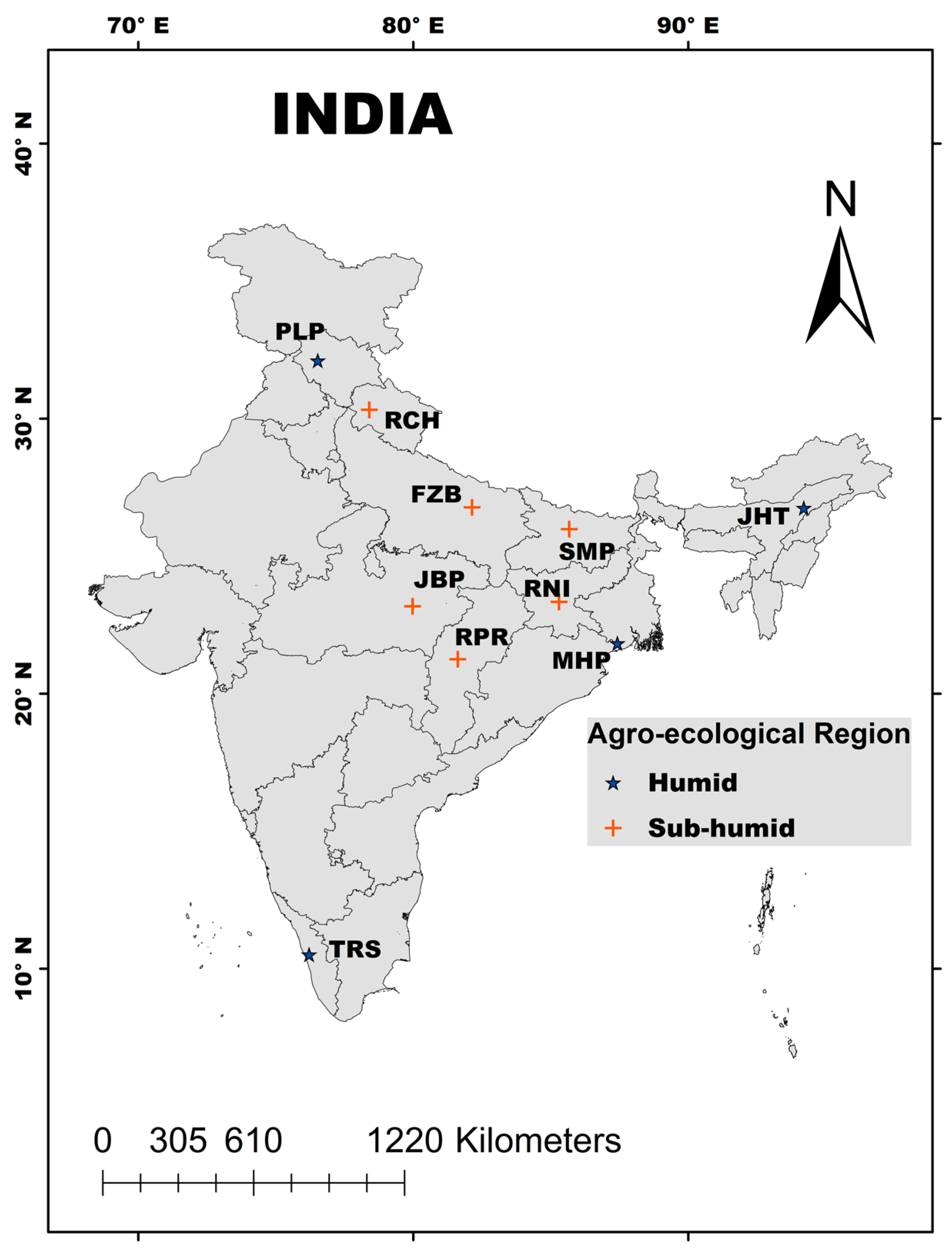
The agro-climatic data of sub-humid and humid regions of India were collected from the All India coordinated research project on Agro-meteorology, ICAR, from 2001 to 2020. The locations wherein the data were collected are depicted in Figure 1. The details of the stations are described in Table 1. The elevations of these stations varied from 17 m in Mohanpur to 1800 m in Ranichauri. The daily meteorological data consisting of maximum air temperature (°C), minimum air temperature (°C), mean relative humidity (%), wind speed at 2 m height (m/s), and the number of sunshine hours were collected from the ten locations from both the regions.
These meteorological parameters affect the evapotranspiration rate by imparting the energy required for vaporization and the rate of water vapour removal from the evaporating surface. The air temperature surrounding the plant impacts the sensible heat of the air. The humidity data would affect the difference in the vapour power of the air and the evaporating surface. The wind speed affects the vapour removal, thereby affecting the evaporation rate. The sunshine data are utilized to calculate the solar radiation, which mostly affects the vaporization of the water to vapour.
2.2. ET0 Estimaton Using FAO-56 Penman-Monteith and Empirical Equations
The ASCE Committee on Irrigation and Water requirements analysed different methods in estimating ET0. They found that the FAO 56 Penman-Monteith can be used in all locations. Hence, the standardised equation of reference evapotranspiration is used as the target variable in the modelling stages. The equation for predicting ET0 by FAO 56 Penman-Monteith is given below. The machine learning models were compared with different empirical equations. The estimation of ET0 using different empirical equations using the formulae as described in Table 2.
2.3. Description of Machine Learning Models and Optimizer
2.3.1. Random Forest (RF)
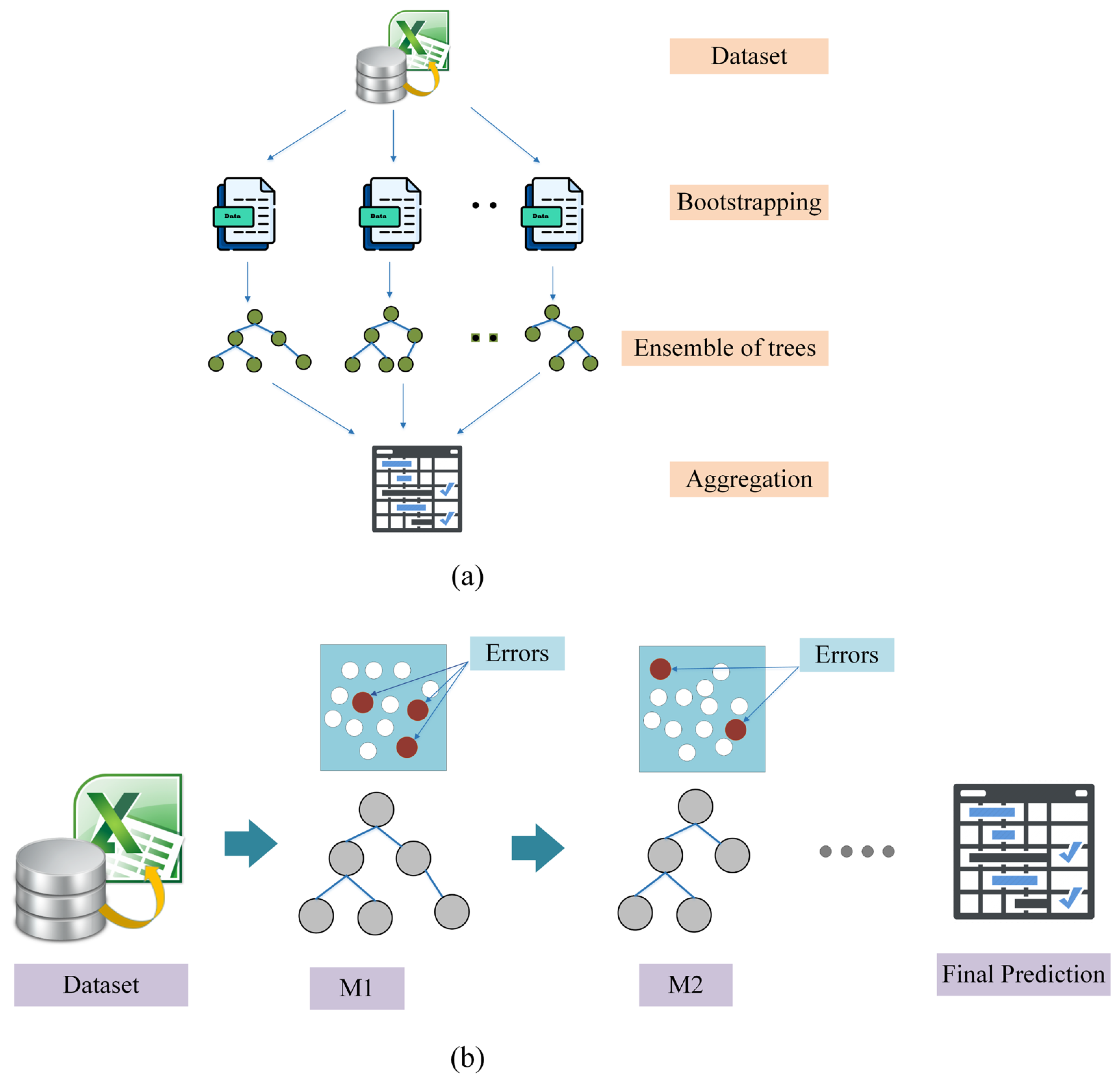
RF model generates output predictions by combining results from several regression decision trees. RF is capable of capturing complex, non-linear interactions between the features and produces a powerful prediction model. Being an ensemble method, RF trains several decision trees in parallel with bootstrapping followed by aggregation (Figure 2a). The trees in the ‘forest’ are generated based on a random selection of subset data from the training set, and the bootstrapping ensures that each tree in the forest is unique [45,46]. For the final prediction, the RF regressor aggregates the decision made by individual trees. RF is robust to outliers, produces better generalization, and has easily tunable hyperparameters [47].
2.3.2. Extreme Gradient Boosting Model (XGB)
XGB provides an efficient and scalable implementation of gradients boosting framework [48] suitable for both regression and classification problems. A typical gradient-boosting approach is an ensemble of decision trees that are trained in a sequential manner [49]. In gradient boosting, a better model is built by merging previous models until the best model reduces the cumulative prediction error (Figure 2b). XGB was developed with optimized and supports distributed computing, additionally improving flexibility and portability. XGB leverages parallel computation to build trees across different processing units. The algorithm supports effective pruning of trees for improving the computational speed and sparsity-aware split finding to handle the missing data.
2.3.3. Light Gradient Boosting Model (LGB)
The LGB model is a gradient-boosting framework built on decision trees that boosts the model’s effectiveness and consumes less memory. The key characteristic of LGB is that the trees are grown leaf-wise instead of checking all of the previous leaves for each new leaf [50]. LGB uses two novel approaches, viz., Gradient-based One Side Sampling and Exclusive Feature Bundling (EFB), to achieve improved performance. Using the GOSS, the major portion of the data points with small gradients are eliminated from calculating the information gain, achieving significant time saving [51]. Using EFB, the mutually exclusive features are bundled, achieving feature reduction without compromising the model performance. The model works effectively on benchmark datasets with increased training speed compared to the conventional gradient-boosting methods.
2.3.4. Grey Wolf Optimizer (GWO)
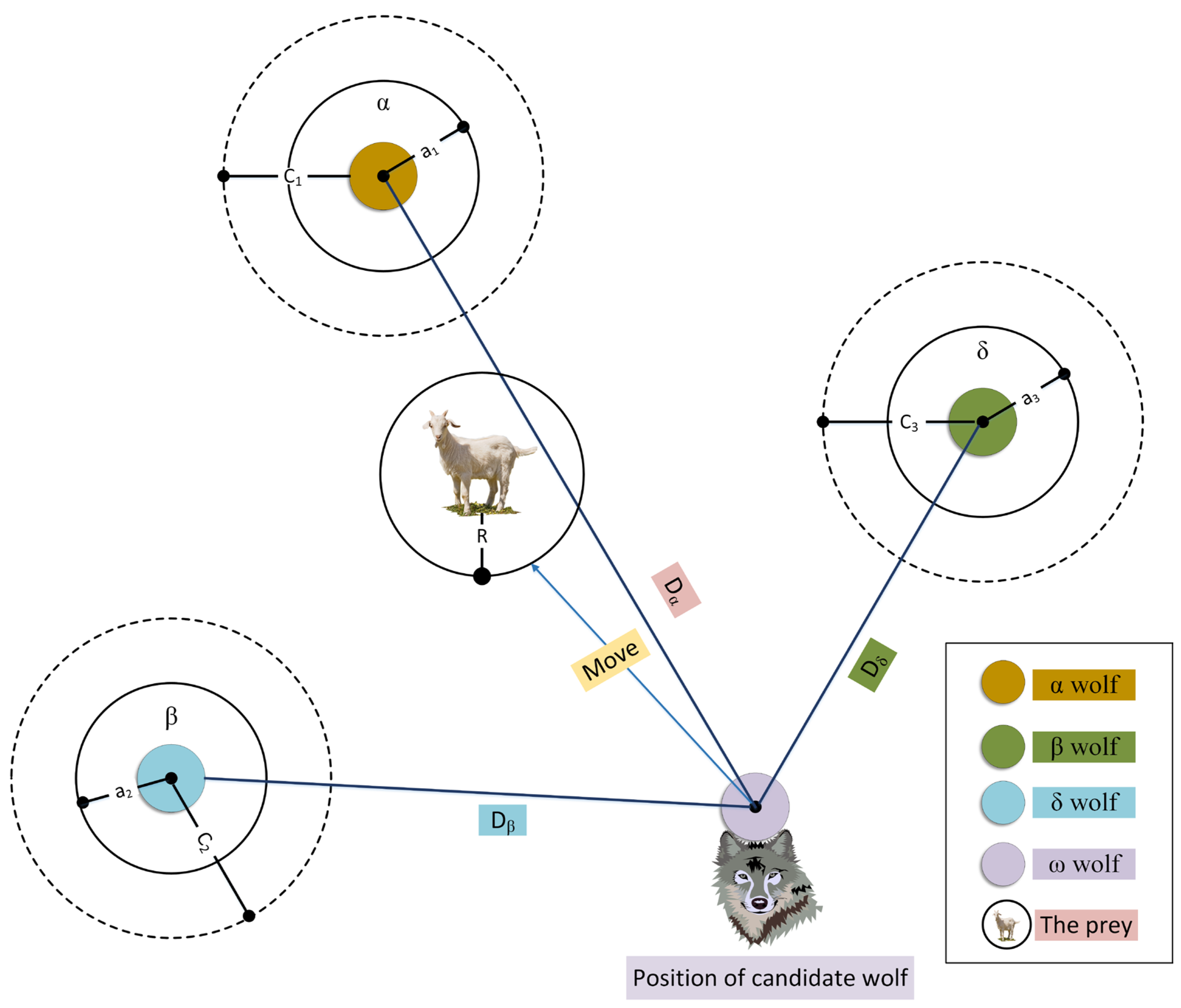
GWO is an evolutionary, meta-heuristic algorithm inspired by the structure of the leadership hierarchy and hunting mechanism of grey wolves in nature [52] and has been proven to be a more practical and precise method for optimization problems [53]. It has significant advantages over the other swarm intelligence approaches, such as a reduced number of parameters and no requirement of derivation information during the initial search, etc. [54]. In GWO, a grey wolf herd’s members are classified as α, β, δ and ω and depending on the effectiveness, decision-making ability, and way of advancing in the hunting process.
The α wolves are the strongest and most powerful, usually serves as the herd’s leader and should be obeyed by the other wolves in the pack. β wolves act as advisors to the alpha group, and δ wolves act in the group as guards, sentinels, and hunters. The ω group of wolves is in the lowest position of decision-making [55] and follows others. The alpha in GWO is believed to be the best answer. In order of priority, the beta, gamma, and omega solutions come next. The wolves in GWO iterations assess the potential for a hunt and adjust their status accordingly (Figure 3).
2.4. ET0 Estimaton Using ML and Hybrid ML
2.4.1. Input Scenarios
The daily meteorological parameters from 2001 to 2020 at all ten stations are used as the inputs for the modelling of daily ET0. The inputs consisted of maximum air temperature (Tmax, °C), minimum air temperature (Tmin, °C), mean relative humidity (RH, %), wind speed at 2 m height (u2, m/s), number of sunshine hours (n, hours), solar radiation (Rn, MJ/m2 day) and extra-terrestrial radiation (Ra, MJ/m2 day).
A total of 18 combinations were employed. Table 3 depicts the different combinations used, ranging from two inputs in model index 1 to six inputs in model indices 17 and 18. The target for these models was the daily ET0 calculated from the FAO-56 Penman-Monteith equation. The statistical indicators of the inputs and output at various stations are presented in Figure S1. The time series graphs of ET0 from some stations of the study on a daily basis from 2001 to 2020 were shown in Figure S2 (Supplementary Materials).
2.4.2. Model Development
The data were normalised, which gives scale uniformity, improving the modelling capability. The normalised input data were used for modelling purposes [57]. The equation used for the normalisation of the data is given below:
where: xnorm is the normalised value of the input, x0 is the actual value of the input that is being normalised, and xmax and xmin are the maximum and minimum values of all the inputs.
Fivefold cross-validation was employed in each of the ML and hybrid ML models, as shown in Table 4. For example, say in the V1 scenario, 16-year daily data from 2005 to 2020 would be used for the model training, and the rest of the data from 2001 to 2004 would be used for the testing of the model developed. This was done for the rest of the cross-validation stages as well so that the whole of the data set would be tested for accuracy. The employment of cross-validation has been found to reduce the over-fitting of the models [24].
2.4.3. Hyper Parameter Tuning in Hybrid ML
The hybrid ML models were developed by optimization of the hyperparameters of RF, XGB, and LGB models using the GWO algorithm. The default values and the range of hyperparameters used in the study are shown in Table 5. The default values of the hyperparameters were used in the state-of-the-art ML models, whereas the best hyperparameter set in each of the ML models was assessed using the GWO to develop the hybrid models, i.e., GWORF, GWOXGB, and GWOLGB. The fine-tuning of hyperparameters could potentially improve the prediction accuracy of hybrid models [58].
2.5. Model Performance Indicators
The indicators used in the study were root mean square error (RMSE), coefficient of determination (R2), mean absolute error (MAE) [27], and agreement index (d) [59]. The formulae for these indicators are described in Table 6.
Global Performance Indicator (GPI)
Using different indicators renders a problem in properly selecting or judging the best models. Hence, a summative index that uses the equation called Global Performance Indicator is used in the study [36]. All the above indicators, i.e., RMSE, R2, MAE, d, were normalized between 0 and 1 using Equation (22), and the value of GPI for a model is found using Equation (23). Higher values of GPI would give the best model compared to other models [60,61].
Nj is the normalized statistical index, Sj is the original statistical index, min(S) is the minimum value in that statistical index, and max(S) is the maximum value in that statistical index.
GPIi is the value of the Global Performance Indicator for model i, Sj is the median value of the statistical indicator j, Sij is the value of the statistical indicator j for model i, αj is a constant with a value of −1 for R2, d and 1 for MAE, RMSE. The ranking based on the GPI value was also done.
3. Results
3.1. Comparison of the Empirical Models in Estimating ET0
Evaluation of different empirical models was carried out against the FAO-56 Penman-Method as the target for the daily data of 20 years at both humid and sub-humid locations. The performance indicators of the fifteen models at humid and sub-humid stations were presented in Tables S1 and S2, respectively. The ranking of the various models at humid stations based on the GPI is depicted in Table 7. The comparison at various stations suggests that the radiation-based models were superior at most stations. In contrast, mass-transfer-based models were found to be of low accuracy. It shows that the Turc Model was a promising method compared to other models. It was followed by Makkink, Valiantzas 2, Jensen-Haise. The lowest-performing empirical models in the humid region were McGuinness-Bordne, Mahringer, and Valiantzas 1. The ranking of the various models at sub-humid stations is shown in Table 8. The superior models in sub-humid regions were Turc, Valiantzas 2, Jensen-Haise, and Preistly-Taylor. The worst empirical models at sub-humid stations were Valiantzas 1, Albrecht, Copias, and Mahringer. The results indicated that the empirical model performance varied at different stations. Overall, the Turc model could be used in the study area based on its superior ranking in most stations.
3.2. Comparison of Various Input Combinations in Conventional ML Models
3.2.1. Best-Performing Models in ML
The three conventional models used in the study, i.e., RF, XGB, and LGB, were evaluated with various input combinations. The results in these sections are for the testing data sets in all the cross-validation stages. The statistical indicators at each station using the conventional ML models are given in Tables S3–S12. It was observed that the R2 value has improved with higher inputs, and LGB models were more accurate than other models. A substantial increase in the accuracy and reduced errors was observed in model indices 8 and 9 across all the stations. The ranking of the eighteen best models (six models in each ML) at humid locations based on the GPI is shown in Table 9. The results indicated that the models that used the most inputs (Index 17 and 18) were superior with higher GPI. The LGB17 and LGB18 performed best in Palampur and Thrissur, whereas the XGB17 was the best at Jorhat and Mohanpur. It was observed that the XGB8 and LGB8, which used wind speed and solar radiation data, performed better in all the stations except Palampur, where the LGB7, RF7, and XGB7 gave accurate estimates. Overall, the performance of RF was found to be inferior to both XGB and LGB. The lowest error (RMSE = 0.096 mm/day) was found using XGB17 at Mohanpur station and, the highest R2 value (0.994) was observed at Palampur and Thrissur for LGB18 and at Mohanpur for LGB17.
The eighteen best-ranking models at sub-humid locations are shown in Table 10. It could be seen that the LGB17 and LGB18 were the best performing at all the six stations. The performance of the model indices 8, 9, and 16 was quite promising at all the stations except at Ranichauri, wherein the index 7 models were accurate. It was observed that the addition of solar radiation as an input considerably increased the performance of the models. The models that correlated with the FAO-56 Penman-Monteith are in the order of LGB, XGB, and RF. The LGB18 at Jabalpur station performed well (R2 = 0.995), whereas the least RMSE (0.094 mm/day) was recorded at Ranichauri for LGB17.
3.2.2. Least-Performing Models in ML
The ranking of the low-performing models at humid locations of all the conventional model and their input combinations are shown in Table 11. The results showed that model indices 1, 2, 3, and 6 were the least ranked models. It was obvious that the model that used the least number of inputs (only temperature data) was the worst model in estimating ET0. The RF models had the lowest GPI values compared to other models’ counterparts at most stations, indicating their higher errors. It was observed that the LGB models performed better than other ML models using the same input combinations. The error was found to be highest (RMSE = 0.919 mm/day) at Thrissur using RF1, whereas the least R2 (0.371) was seen at Jorhat for RF1. The model combination that used extra-terrestrial radiation, i.e., model indices 10 and 11, did not yield accurate results.
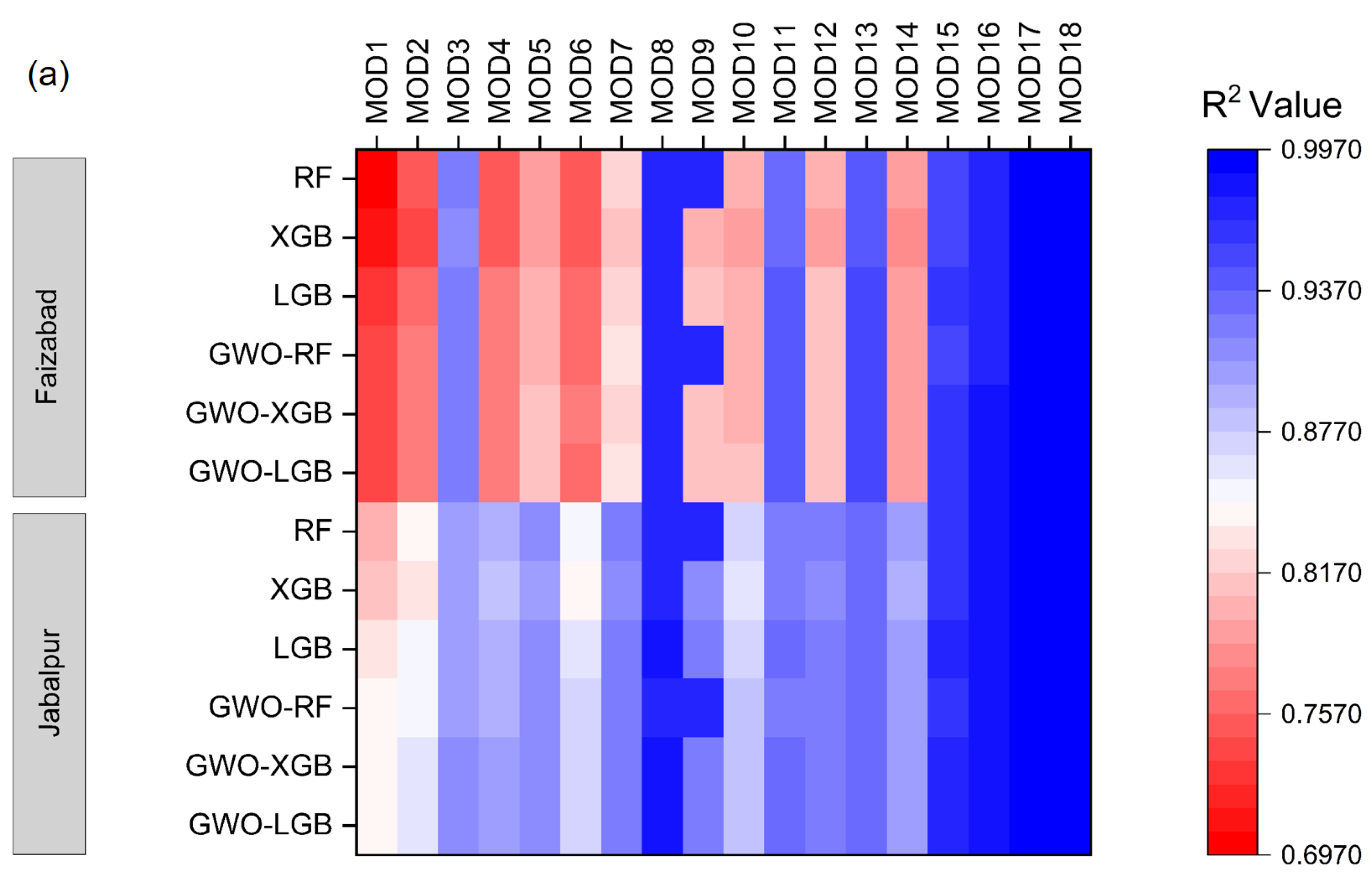
The results at the sub-humid stations were found to be quite similar to that of humid locations (Table 12). The model indices 1, 2, 6, and 3 were ranked the lowest in most stations. The highest RMSE of 1.253 mm/day was observed at Faizabad station using the RF1 model, whereas the lowest R2 (0.631) was reported at Samastipur with the same set of ML model.
3.3. Empirical Models v/s Conventional ML Models
The conventional ML models were compared with the empirical equations that employed a similar combination of inputs for modelling. The results at humid (Table 13) and sub-humid locations (Table 14) depicted that the ML models outperformed the empirical models with high GPI values at all combinations and locations. It could be observed that in indices 13, 5, 6, and 7, the models performed in the order of LGB, RF, and XGB.
3.4. Comparison of Various Input Combinations in GWO Hybrid ML Models
3.4.1. Best-Performing Models in Hybrid ML
The results of the best hyperparameters in each of the models are attached in Tables S13 to S18. These hyperparameters were used to develop the hybrid ML models at all the stations of humid and sub-humid zones. The statistical indicators at each of the stations using the hybrid ML models are given in Tables S19–S28. The six accurate models in each of the ML models were employed in assessing the best-performing models. The ranking of the best of all the hybrid ML models and their combinations at humid locations based on the GPI is shown in Table 15. The results indicated that the models that used the most inputs (Index 17 and 18) were superior with higher GPI. The GWOXGB17 and GWOXGB18 performed best in all the stations, whereas the GWOLGB18 was the second best at Palampur and Thrissur. It was observed that indices 7, 8, and 9, which solar radiation data performed better in most of the stations. The superiority of RF models in these combinations was observed in all the stations except at Thrissur. The performance of the model GWOXGB18 at Thrissur was the best of the models with an RMSE of 0.073 mm/day and R2 of 0.997.
Of the 54 hybrid models evaluated, the eighteen best-ranking hybrid ML models at sub-humid locations are shown in Table 16. The performance of the models was in the order of indices: 17, 18, and 16 at the Faizabad, Jabalpur, and Raipur stations. The accuracy of the models with indices 7, 8, and 9 is also high compared to the models that used a higher number of inputs. This could be attributed to the incorporation of solar radiation data. The model indices 15 and 13 also found a place in the best-performing models, with wind speed as a common input. The lowest RMSE (0.083 mm/day) was observed at Ranichauri, which used GWOLGB17, while the R2 was found to be the highest (0.997) at Jabalpur for both GWOLGB18 and GWOLGB17. The overall performance of the hybrid models is in the order of GWOXGB > GWOLGB > GWORF at most stations.
3.4.2. Least Performing Models in Hybrid ML
The least-performing models of the hybrid ML at humid stations are presented in Table 17. The six least accurate models in each hybrid ML, i.e., GWORF, GWOXGB, and GWOLGB, were used to analyse all the combinations. The models with the lowest GPI values were found in the order of the model indices 1, 3, and 6 in all the hybrid ML at most stations. The models with indices 10 and 11 that used extra-terrestrial radiation as input were also placed in the least-ranking hybrid models at all the stations. There was no specific order found in the accuracy of the various models. The performance ranking of the least accurate hybrid models is given in Table 18. The model GWORF1 at Thrissur station gave the highest RMSE (0.812 mm/day) of all the models, whereas the lowest R2 (0.478) was observed at Jorhat stations with the same model combination.
The least ranked models in the sub-humid stations were similar to that of the results of humid stations. Models 1, 2, 3, and 6 were the least accurate in most sub-humid locations. Of the four input combination methods, the models with the indices 10, 14, 11, and 13 found a place in the least ranked models. The performance of the different hybrid models did not show any specific trend at this level of comparison in all the stations. The error was observed highest (1.154 mm/day) at Faizabad for both GWOLGB1 and GWOXGB1. The R2 was found to be the least at Samastipur station, with a value of 0.693. The RF models have got the advantage of improving their efficiency by the hyperparameter tuning by GWO than the XGB and LGB models.
3.5. Best-Performing Models across Conventional and Hybrid MLs
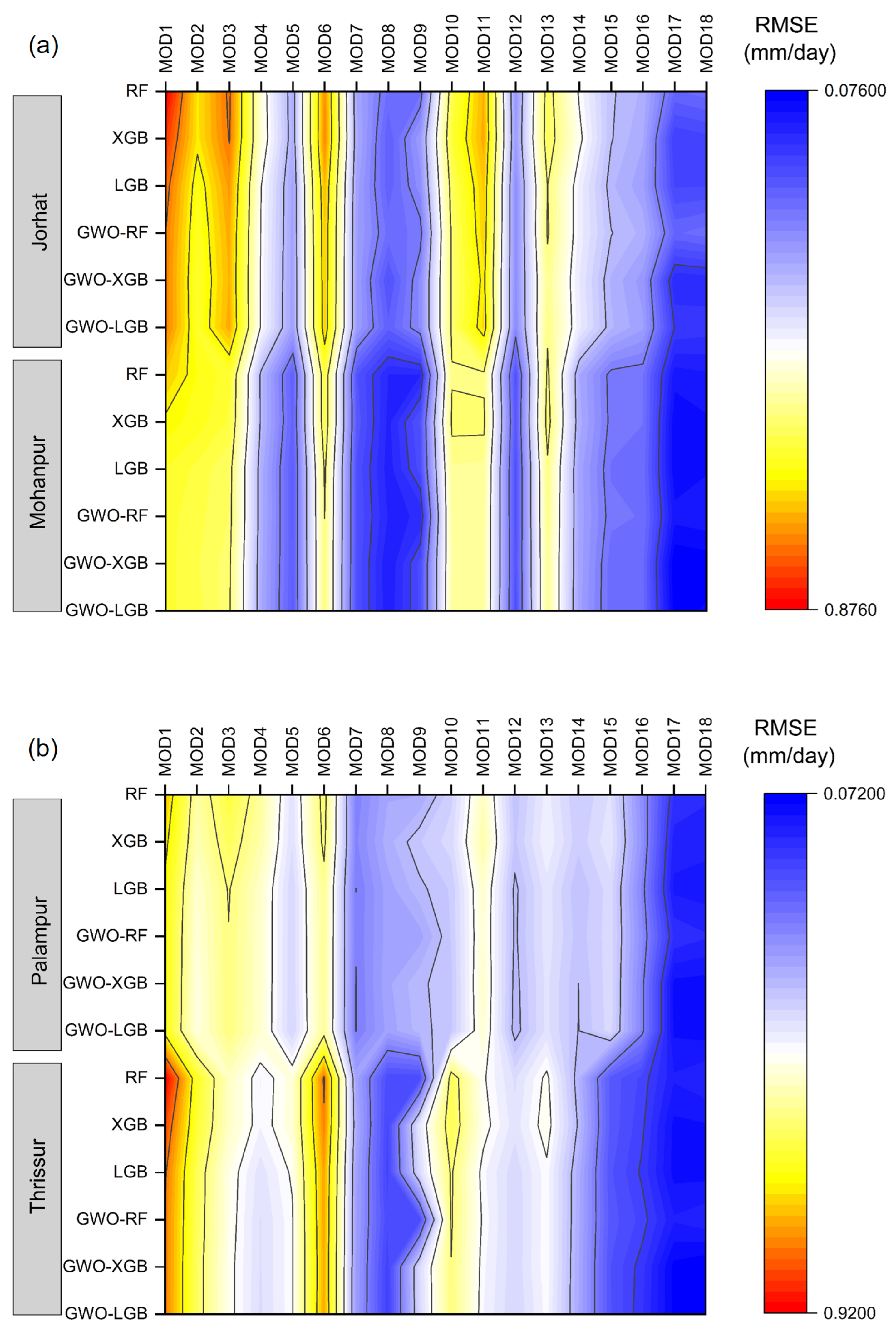
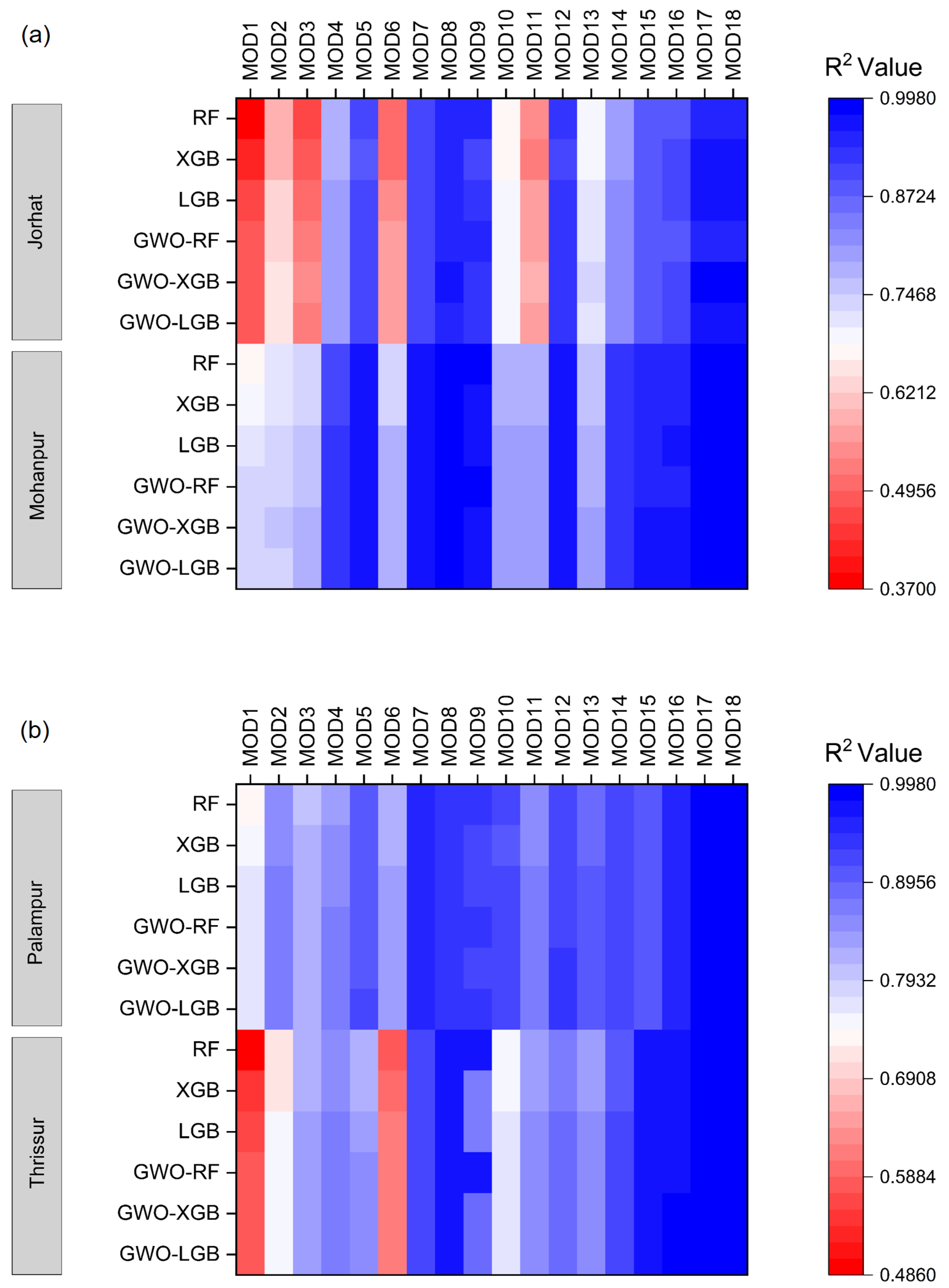
Table 19 depicts the best 36 models out of 108 models that compare all the conventional and hybrid ML at humid locations. The plots showing the RMSE and R2 at different locations in the humid region are shown in Figure 4 and Figure 5, respectively. The results indicate that the hybrid models outperformed their conventional ML counterparts in most of the combinations. The models that used the six inputs were the superior, followed by the models with indices 7, 8, 9, 16, and 12. The accuracy of the XGB and LGB models was higher than RF models at almost all stations. The use of solar radiation could be attributed to the excellent performance of models 7, 8, and 9 than the other models that have employed more inputs.
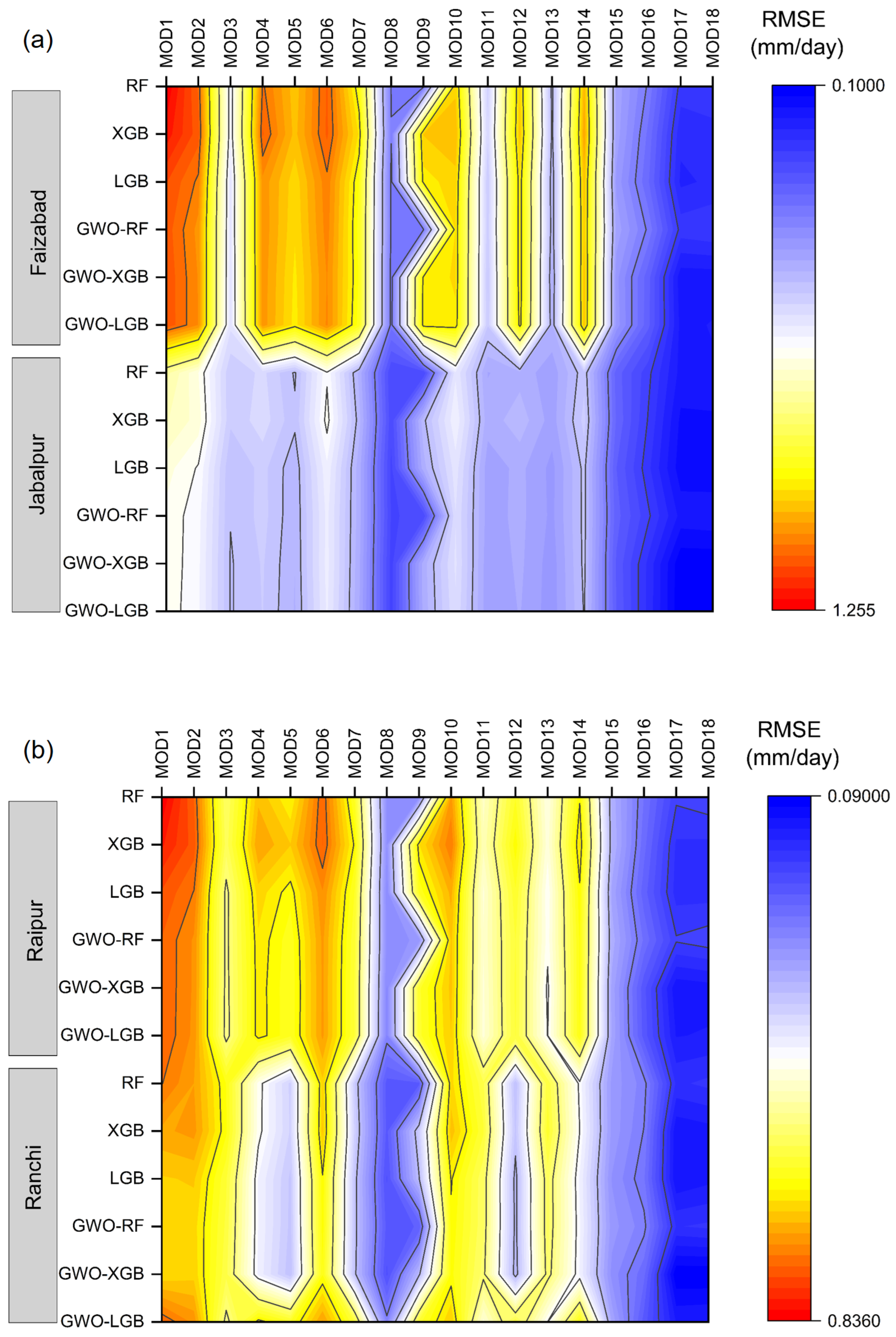
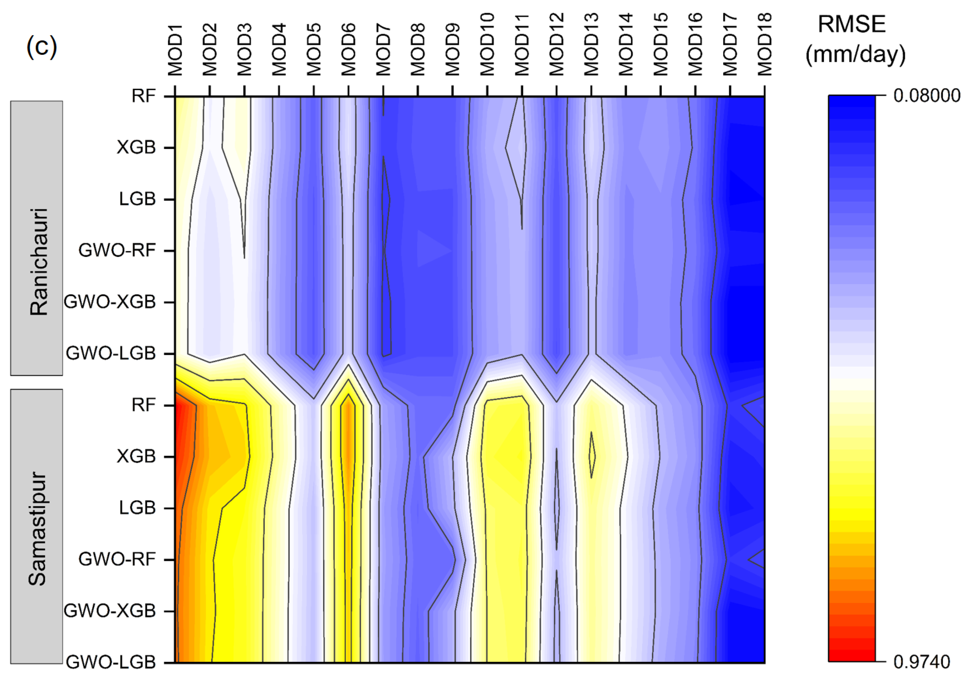
The results of the overall best-performing models in conventional and hybrid models at the sub-humid stations are presented in Table 20. The plots showing the RMSE and R2 at different locations in the humid region are shown in Figure 6 and Figure 7, respectively. The observed results at the sub-humid locations were in good resonance with that of the humid locations. The models with indices 17, 18, and 16 were also predicting with greater accuracy at these locations. The solar radiation data used in models 7, 8, and 9 were also ranked best in comparison. The application of GWO has improved the accuracy of the ML models in all the combinations at all stations. The higher GPI values were observed in LGB and XGB when compared with the RF models using a similar set of inputs.
3.6. Least-Performing Models across Conventional and Hybrid MLs
Based on the least GPI values, the six least-performing models from each conventional and hybrid ML model were combined to assess the ranking of all the models. Table 21 illustrates the worst ranking models at the humid stations. It was observed from the results that the models with indices 1, 2, 3, and 6 were found to be the least-ranked models. The conventional ML models were less accurate than their hybrid models. In most instances, the XGB and LGB models were slightly more accurate than the RF models. A similar observation was noted at sub-humid locations, tabulated in Table 22. The combination of inputs that consisted of two and three inputs was the least ranked at almost all the stations. The advantage of using hybrid models could be seen with the higher GPI values of those models than the conventional ML models. The results at sub-humid locations also indicate the inferior accuracy of RF when compared to the boosting models, i.e., LGB and XGB. The addition of extra-terrestrial radiation did not increase the accuracy of the models to a greater extent, which could be observed from the model indices 10 and 11 securing least ranking than other 4-input combination models.
4. Discussion
Reference evapotranspiration estimation is essential in various applications ranging from agricultural water management, hydrological balancing across basins and water allocation, etc. The study used various empirical, ML and hybrid ML models that were tested across the humid and sub-humid stations across the Indian subcontinent. Among empirical equations, the Turc model was found to be the most reliable method in empirical models used. Similar results were reported in [62,63], wherein the radiation-based Turc model performed better. Many studies have proven that the empirical equations underperformed the ML models, which was also observed in this study. [64] assessed different artificial intelligence models with empirical models like Turc, Ritchie, Thornthwaite, and Valiantzas methods. Their results indicated the supremacy of the ML models in predicting ET0. The comparison between the conventional ML models based on the performance indicators showed that the XGB and LGB models showed similar accuracies. [30] have also indicated that both of these models exhibited the same model efficacy. The boosting methods were to be a potential tool for humid regions according to [65]. RF models were found to be less accurate than the other boosting models, as reported in [24,29].
The model accuracy increased as increasing the inputs, which was exhibited in most of the studies. The models that used solar radiation have performed reasonably well in both the regions, i.e., humid and sub-humid. [29] also found that the addition of solar radiation improved the accuracy. The models in the sub-humid regions that used wind speed data were found to be of better accuracy. These results were similar that were found in Bangladesh [64]. The best and least performing models’ results have been found to vary slightly across the stations. However, the four input combination models, indices 7 and 8, were found to be consistently performing well in both regions. Applying these data-driven models with lower inputs could be promising for developing nations.
The hybrid ML models further enhanced the predictability of the models, which could be possible by proper hyperparameter tuning. This is evident from the observation of the improvement in the GWORF model performance over the conventional RF. RF models showed a greater improvement due to the optimization than the XGB and LGB models. A similar study by [61] reported an improvement in all the combinations of inputs when employing PSO. The hyperparameter values varied considerably in all the combinations and stations. There is no fixed set of hyperparameters for all the ML models and their input combinations that could be suggested for optimal results, as suggested in [36]. Nevertheless, these models have proven to be of good accuracy, and there is a scope for further improvement if different optimizers could be tested across the regions of the World.
5. Conclusions
This study evaluated the ET0 modelling capabilities of tree-based ML like RF, XGB, and LGB in addition to the GWO-optimized tree-based ML for ten locations in humid and sub-humid regions across India. The daily data from 2001 to 2020 of agro-meteorological parameters like maximum temperature, minimum temperature, wind speed, relative humidity, number of sunshine hours, solar radiation and extra-terrestrial radiation were employed for modelling purposes. The FAO-56 Penman-Monteith was used as the target value. Different input combinations were tested at all the stations using a cross-validation strategy. The comparison of the empirical equations was also made for the ML that used the same input combinations. The ranking of the models based on GPI value for comparison at each level was considered. The conclusions that could be drawn from the study are below.
- The LGB and XGB models outperformed the RF models, while all the ML models were found to be more accurate than empirical models.
- Among the empirical methods investigated in the study, the Turc model was determined to have the greatest performance with higher GPI values.
- Solar radiation was adjudged to be an important parameter that could improve the prediction capability.
- The GWO hybrid ML models had the highest prediction efficiencies at all the locations, with RF models improving considerably well.
- The study consolidated the fact that the use of optimizers would substantially reduce the modelling error.
- Further studies could be done using cross-station data and other optimizers to improve the accuracy.
Supplementary Materials
The following supplementary information can be downloaded at: https://www.mdpi.com/article/10.3390/w15050856/s1, Figure S1. Statistical indicators of inputs and output used in the study; Figure S2. Time series graphs of ET0 (mm/day) at humid (Jorhat, Thrissur) and sub-humid (Raipur, Samastipur) stations; Table S1. Performance indicators of empirical models at humid stations; Table S2. Performance indicators of empirical models at sub-humid stations; Table S3. Performance indicators of conventional ML models at Jorhat; Table S4. Performance indicators of conventional ML models at Mohanpur; Table S5. Performance indicators of conventional ML models at Palampur; Table S6. Performance indicators of conventional ML models at Thrissur; Table S7. Performance indicators of conventional ML models at Faizabad; Table S8. Performance indicators of conventional ML models at Jabalpur; Table S9. Performance indicators of conventional ML models at Raipur; Table S10. Performance indicators of conventional ML models at Ranchi; Table S11. Performance indicators of conventional ML models at Ranichauri; Table S12. Performance indicators of conventional ML models at Samastipur; Table S13. Best hyper parameters in RF models at humid stations; Table S14. Best hyper parameters in XGB models at humid stations; Table S15. Best hyper parameters in LGB models at humid stations; Table S16. Best hyper parameters in RF models at sub-humid stations; Table S17. Best hyper parameters in XGB models at sub-humid stations; Table S18. Best hyper parameters in LGB models at sub-humid stations; Table S19. Performance indicators of hybrid ML models at Jorhat; Table S20. Performance indicators of hybrid ML models at Mohanpur; Table S21. Performance indicators of hybrid ML models at Palampur; Table S22. Performance indicators of hybrid ML models at Thrissur; Table S23. Performance indicators of hybrid ML models at Faizabad; Table S24. Performance indicators of hybrid ML models at Jabalpur; Table S25. Performance indicators of hybrid ML models at Raipur; Table S26. Performance indicators of hybrid ML models at Ranchi; Table S27. Performance indicators of hybrid ML models at Ranichauri; Table S28. Performance indicators of hybrid ML models at Samastipur.
Author Contributions
Conceptualization, P.H. and K.V.R.R.; methodology, P.H., K.V.R.R. and A.S. (A. Subeesh); software, P.H., A.S. (A. Subeesh) and A.S. (Ankur Srivatsava); formal analysis, P.H. and K.V.R.R.; investigation, P.H. and A.S. (A. Subeesh); writing—original draft preparation, P.H. and K.V.R.R.; writing—review and editing, K.V.R.R., A.S. (A. Subeesh) and A.S. (Ankur Srivatsava); visualization, A.S. (A. Subeesh) and A.S. (Ankur Srivatsava); supervision, K.V.R.R. All authors have read and agreed to the published version of the manuscript.
Funding
This research received no external funding.
Data Availability Statement
The datasets generated and/or analysed during the current study are available from the corresponding author upon reasonable request.
Acknowledgments
The scholarship to the first author through the ICAR JRF/SRF scholarship from Indian Council of Agricultural Research is highly acknowledged. The authors also thank the AICRP on Agro-meteorology, CRIDA, India for providing the data required.
Conflicts of Interest
The authors declare no conflict of interest.
References
- United Nations Department of Economic and Social Affairs, Population Division. World Population Prospects 2022: Summary of Results; UN DESA/POP/2022/TR/NO. 3; United Nations: New York, NY, USA, 2022. [Google Scholar]
- Lybbert, T.J.; Sumner, D.A. Agricultural Technologies for Climate Change in Developing Countries: Policy Options for Innovation and Technology Diffusion. Food Policy 2012, 37, 114–123. [Google Scholar] [CrossRef]
- Srilakshmi, M.; Jhajharia, D.; Gupta, S.; Yurembam, G.S.; Patle, G.T. Analysis of Spatio-Temporal Variations and Change Point Detection in Pan Coefficients in the Northeastern Region of India. Theor. Appl. Climatol. 2022, 147, 1545–1559. [Google Scholar] [CrossRef]
- George, B.A.; Reddy, B.; Raghuwanshi, N.; Wallender, W. Decision Support System for Estimating Reference Evapotranspiration. J. Irrig. Drain. Eng. 2002, 128, 1–10. [Google Scholar] [CrossRef]
- Srivastava, A.; Sahoo, B.; Raghuwanshi, N. Evaluation of Variable Infiltration Capacity Model and MODIS-Terra Satellite-Derived Grid-Scale Evapotranspiration Estimates in a River Basin with Tropical Monsoon-Type Climatology. J. Irrig. Drain Eng. 2017, 143, 04017028. [Google Scholar] [CrossRef] [Green Version]
- Albrecht, F. Die Methoden zur Bestimmung der Verdunstung der natürlichen Erdoberfläche. Arch. Meteorol. Geophys. Bioklimatol. Ser. B 1950, 2, 1–38. [Google Scholar] [CrossRef]
- Mahringer, W. Verdunstungsstudien am Neusiedler See. Arch. Meteorol. Geophys. Bioklimatol. Ser. B 1970, 18, 1–20. [Google Scholar] [CrossRef]
- Penman, H.L. Natural Evaporation from Open Water, Bare Soil and Grass. Proc. R. Soc. Lond. Ser. Math. Phys. Sci. 1948, 193, 120–145. [Google Scholar]
- Abtew, W. Evapotranspiration Measurements and Modeling for Three Wetland Systems in South Florida1. JAWRA J. Am. Water Resour. Assoc. 1996, 32, 465–473. [Google Scholar] [CrossRef]
- Hansen, S. Estimation of Potential and Actual Evapotranspiration: Paper Presented at the Nordic Hydrological Conference (Nyborg, Denmark, August—1984). Hydrol. Res. 1984, 15, 205–212. [Google Scholar] [CrossRef]
- Rosenberg, N.J.; Blad, B.L.; Verma, S.B. Microclimate: The Biological Environment; John Wiley & Sons: Hoboken, NJ, USA, 1983; ISBN 0-471-06066-6. [Google Scholar]
- McGuinness, J.L.; Bordne, E.F. A Comparison of Lysimeter-Derived Potential Evapotranspiration with Computed Values; US Department of Agriculture: Washington, DC, USA, 1972. [Google Scholar]
- Priestley, C.H.B.; Taylor, R.J. On the Assessment of Surface Heat Flux and Evaporation Using Large-Scale Parameters. Mon. Weather Rev. 1972, 100, 81–92. [Google Scholar] [CrossRef]
- Turc, L. Estimation of Irrigation Water Requirements, Potential Evapotranspiration: A Simple Climatic Formula Evolved up to Date. Ann. Agron. 1961, 12, 13–49. [Google Scholar]
- Hargreaves, G.H. Moisture Availability and Crop Production. Trans. ASAE 1975, 18, 980–0984. [Google Scholar] [CrossRef]
- Hargreaves, G.H.; Samani, Z.A. Reference Crop Evapotranspiration from Temperature. Appl. Eng. Agric. 1985, 1, 96–99. [Google Scholar] [CrossRef]
- Droogers, P.; Allen, R.G. Estimating Reference Evapotranspiration under Inaccurate Data Conditions. Irrig. Drain. Syst. 2002, 16, 33–45. [Google Scholar] [CrossRef]
- Alexandris, S.; Kerkides, P.; Liakatas, A. Daily Reference Evapotranspiration Estimates by the “Copais” Approach. Agric. Water Manag. 2006, 82, 371–386. [Google Scholar] [CrossRef]
- Valiantzas, J.D. Simple ET0 Forms of Penman’s Equation without Wind and/or Humidity Data. II: Comparisons with Reduced Set-FAO and Other Methodologies. J. Irrig. Drain. Eng. 2013, 139, 9–19. [Google Scholar] [CrossRef] [Green Version]
- Jing, W.; Yaseen, Z.M.; Shahid, S.; Saggi, M.K.; Tao, H.; Kisi, O.; Salih, S.Q.; Al-Ansari, N.; Chau, K.-W. Implementation of Evolutionary Computing Models for Reference Evapotranspiration Modeling: Short Review, Assessment and Possible Future Research Directions. Eng. Appl. Comput. Fluid Mech. 2019, 13, 811–823. [Google Scholar] [CrossRef] [Green Version]
- Ayodele, T.O. Machine Learning Overview. New Adv. Mach. Learn. 2010, 2, 9–18. [Google Scholar]
- Shiri, J.; Zounemat-Kermani, M.; Kisi, O.; Mohsenzadeh Karimi, S. Comprehensive Assessment of 12 Soft Computing Approaches for Modelling Reference Evapotranspiration in Humid Locations. Meteorol. Appl. 2020, 27, e1841. [Google Scholar] [CrossRef] [Green Version]
- Bellido-Jiménez, J.A.; Estévez, J.; Vanschoren, J.; García-Marín, A.P. AgroML: An Open-Source Repository to Forecast Reference Evapotranspiration in Different Geo-Climatic Conditions Using Machine Learning and Transformer-Based Models. Agronomy 2022, 12, 656. [Google Scholar] [CrossRef]
- Fan, J.; Yue, W.; Wu, L.; Zhang, F.; Cai, H.; Wang, X.; Lu, X.; Xiang, Y. Evaluation of SVM, ELM and Four Tree-Based Ensemble Models for Predicting Daily Reference Evapotranspiration Using Limited Meteorological Data in Different Climates of China. Agric. For. Meteorol. 2018, 263, 225–241. [Google Scholar] [CrossRef]
- Liu, X.; Wu, L.; Zhang, F.; Huang, G.; Yan, F.; Bai, W. Splitting and Length of Years for Improving Tree-Based Models to Predict Reference Crop Evapotranspiration in the Humid Regions of China. Water 2021, 13, 3478. [Google Scholar] [CrossRef]
- Wu, Z.; Cui, N.; Gong, D.; Zhu, F.; Xing, L.; Zhu, B.; Chen, X.; Wen, S.; Liu, Q. Simulation of Daily Maize Evapotranspiration at Different Growth Stages Using Four Machine Learning Models in Semi-Humid Regions of Northwest China. J. Hydrol. 2022, 617, 128947. [Google Scholar] [CrossRef]
- Zhou, Z.; Zhao, L.; Lin, A.; Qin, W.; Lu, Y.; Li, J.; Zhong, Y.; He, L. Exploring the Potential of Deep Factorization Machine and Various Gradient Boosting Models in Modeling Daily Reference Evapotranspiration in China. Arab. J. Geosci. 2021, 13, 1287. [Google Scholar] [CrossRef]
- Wu, L.; Peng, Y.; Fan, J.; Wang, Y. Machine Learning Models for the Estimation of Monthly Mean Daily Reference Evapotranspiration Based on Cross-Station and Synthetic Data. Hydrol. Res. 2019, 50, 1730–1750. [Google Scholar] [CrossRef] [Green Version]
- Fan, J.; Ma, X.; Wu, L.; Zhang, F.; Yu, X.; Zeng, W. Light Gradient Boosting Machine: An Efficient Soft Computing Model for Estimating Daily Reference Evapotranspiration with Local and External Meteorological Data. Agric. Water Manag. 2019, 225, 105758. [Google Scholar] [CrossRef]
- Wu, T.; Zhang, W.; Jiao, X.; Guo, W.; Hamoud, Y.A. Comparison of Five Boosting-Based Models for Estimating Daily Reference Evapotranspiration with Limited Meteorological Variables. PLoS ONE 2020, 15, e0235324. [Google Scholar] [CrossRef] [PubMed]
- Zhang, H.; Meng, F.; Xu, J.; Liu, Z.; Meng, J. Evaluation of Machine Learning Models for Daily Reference Evapotranspiration Modeling Using Limited Meteorological Data in Eastern Inner Mongolia, North China. Water 2022, 14, 2890. [Google Scholar] [CrossRef]
- Ferreira, L.B.; da Cunha, F.F. New Approach to Estimate Daily Reference Evapotranspiration Based on Hourly Temperature and Relative Humidity Using Machine Learning and Deep Learning. Agric. Water Manag. 2020, 234, 106113. [Google Scholar] [CrossRef]
- Mokari, E.; DuBois, D.; Samani, Z.; Mohebzadeh, H.; Djaman, K. Estimation of Daily Reference Evapotranspiration with Limited Climatic Data Using Machine Learning Approaches across Different Climate Zones in New Mexico. Theor. Appl. Climatol. 2022, 147, 575–587. [Google Scholar] [CrossRef]
- Wu, T.; Zhang, W.; Jiao, X.; Guo, W.; Alhaj Hamoud, Y. Evaluation of Stacking and Blending Ensemble Learning Methods for Estimating Daily Reference Evapotranspiration. Comput. Electron. Agric. 2021, 184, 106039. [Google Scholar] [CrossRef]
- Yan, S.; Wu, L.; Fan, J.; Zhang, F.; Zou, Y.; Wu, Y. A Novel Hybrid WOA-XGB Model for Estimating Daily Reference Evapotranspiration Using Local and External Meteorological Data: Applications in Arid and Humid Regions of China. Agric. Water Manag. 2021, 244, 106594. [Google Scholar] [CrossRef]
- Maroufpoor, S.; Bozorg-Haddad, O.; Maroufpoor, E. Reference Evapotranspiration Estimating Based on Optimal Input Combination and Hybrid Artificial Intelligent Model: Hybridization of Artificial Neural Network with Grey Wolf Optimizer Algorithm. J. Hydrol. 2020, 588, 125060. [Google Scholar] [CrossRef]
- Dong, J.; Liu, X.; Huang, G.; Fan, J.; Wu, L.; Wu, J. Comparison of Four Bio-Inspired Algorithms to Optimize KNEA for Predicting Monthly Reference Evapotranspiration in Different Climate Zones of China. Comput. Electron. Agric. 2021, 186, 106211. [Google Scholar] [CrossRef]
- Devendra, C.; Thomas, D. Crop–Animal Systems in Asia: Importance of Livestock and Characterisation of Agro-Ecological Zones. Agric. Syst. 2002, 71, 5–15. [Google Scholar] [CrossRef]
- Mandal, D.; Mandal, C.; Singh, S. Delineating Agro-Ecological Regions. ICAR-NBSSLUP Technol. 2016, 1–8. [Google Scholar]
- Allen, R.G.; Pereira, L.S.; Raes, D.; Smith, M. Crop Evapotranspiration-Guidelines for Computing Crop Water Requirements-FAO Irrigation and Drainage Paper 56. FAO Rome 1998, 300, D05109. [Google Scholar]
- Tabari, H.; Grismer, M.E.; Trajkovic, S. Comparative Analysis of 31 Reference Evapotranspiration Methods under Humid Conditions. Irrig. Sci. 2013, 31, 107–117. [Google Scholar] [CrossRef]
- Xystrakis, F.; Matzarakis, A. Evaluation of 13 Empirical Reference Potential Evapotranspiration Equations on the Island of Crete in Southern Greece. J. Irrig. Drain. Eng. 2011, 137, 211–222. [Google Scholar] [CrossRef] [Green Version]
- Rosenberry, D.O.; Stannard, D.I.; Winter, T.C.; Martinez, M.L. Comparison of 13 Equations for Determining Evapotranspiration from a Prairie Wetland, Cottonwood Lake Area, North Dakota, USA. Wetlands 2004, 24, 483–497. [Google Scholar] [CrossRef]
- Bourletsikas, A.; Argyrokastritis, I.; Proutsos, N. Comparative Evaluation of 24 Reference Evapotranspiration Equations Applied on an Evergreen-Broadleaved Forest. Hydrol. Res. 2017, 49, 1028–1041. [Google Scholar] [CrossRef]
- Breiman, L. Random Forests. Mach. Learn. 2001, 45, 5–32. [Google Scholar] [CrossRef] [Green Version]
- Smith, P.F.; Ganesh, S.; Liu, P. A Comparison of Random Forest Regression and Multiple Linear Regression for Prediction in Neuroscience. J. Neurosci. Methods 2013, 220, 85–91. [Google Scholar] [CrossRef] [PubMed]
- Misra, S.; Li, H. Chapter 9—Noninvasive Fracture Characterization Based on the Classification of Sonic Wave Travel Times. In Machine Learning for Subsurface Characterization; Misra, S., Li, H., He, J., Eds.; Gulf Professional Publishing: Houston, TX, USA, 2020; pp. 243–287. ISBN 978-0-12-817736-5. [Google Scholar]
- Chen, T.; He, T.; Benesty, M.; Khotilovich, V.; Tang, Y.; Cho, H.; Chen, K. Xgboost: Extreme Gradient Boosting. In R Package; Version 04-2; R Foundation for Statistical Computing: Vienna, Austria, 2015; Volume 1, pp. 1–4. [Google Scholar]
- Friedman, J.H. Greedy Function Approximation: A Gradient Boosting Machine. Ann. Stat. 2001, 29, 1189–1232. [Google Scholar] [CrossRef]
- Al Daoud, E. Comparison between XGBoost, LightGBM and CatBoost Using a Home Credit Dataset. Int. J. Comput. Inf. Eng. 2019, 13, 6–10. [Google Scholar]
- Ke, G.; Meng, Q.; Finley, T.; Wang, T.; Chen, W.; Ma, W.; Ye, Q.; Liu, T.-Y. LightGBM: A Highly Efficient Gradient Boosting Decision Tree. In Proceedings of the Advances in Neural Information Processing Systems, Long Beach, CA, USA, 4–9 December 2017; Curran Associates, Inc.: Red Hook, NY, USA, 2017; Volume 30. [Google Scholar]
- Mirjalili, S.; Mirjalili, S.M.; Lewis, A. Grey Wolf Optimizer. Adv. Eng. Softw. 2014, 69, 46–61. [Google Scholar] [CrossRef] [Green Version]
- Sweidan, A.H.; El-Bendary, N.; Hassanien, A.E.; Hegazy, O.M.; Mohamed, A.E. Water Quality Classification Approach Based on Bio-Inspired Gray Wolf Optimization. In Proceedings of the 2015 7th International Conference of Soft Computing and Pattern Recognition (SoCPaR), Fukuoka, Japan, 13–15 November 2015; pp. 1–6. [Google Scholar]
- Faris, H.; Aljarah, I.; Al-Betar, M.A.; Mirjalili, S. Grey Wolf Optimizer: A Review of Recent Variants and Applications. Neural Comput. Appl. 2018, 30, 413–435. [Google Scholar] [CrossRef]
- Mohammadi, B.; Guan, Y.; Aghelpour, P.; Emamgholizadeh, S.; Pillco Zolá, R.; Zhang, D. Simulation of Titicaca Lake Water Level Fluctuations Using Hybrid Machine Learning Technique Integrated with Grey Wolf Optimizer Algorithm. Water 2020, 12, 3015. [Google Scholar] [CrossRef]
- Sharma, I.; Kumar, V.; Sharma, S. A Comprehensive Survey on Grey Wolf Optimization. Recent Adv. Comput. Sci. Commun. Former. Recent Pat. Comput. Sci. 2022, 15, 323–333. [Google Scholar]
- Feng, Y.; Cui, N.; Zhao, L.; Hu, X.; Gong, D. Comparison of ELM, GANN, WNN and Empirical Models for Estimating Reference Evapotranspiration in Humid Region of Southwest China. J. Hydrol. 2016, 536, 376–383. [Google Scholar] [CrossRef]
- He, H.; Liu, L.; Zhu, X. Optimization of Extreme Learning Machine Model with Biological Heuristic Algorithms to Estimate Daily Reference Evapotranspiration in Hetao Irrigation District of China. Eng. Appl. Comput. Fluid Mech. 2022, 16, 1939–1956. [Google Scholar] [CrossRef]
- Heramb, P.; Kumar Singh, P.; Ramana Rao, K.V.; Subeesh, A. Modelling Reference Evapotranspiration Using Gene Expression Programming and Artificial Neural Network at Pantnagar, India. Inf. Process. Agric. 2022; in press. [Google Scholar] [CrossRef]
- Despotovic, M.; Nedic, V.; Despotovic, D.; Cvetanovic, S. Review and Statistical Analysis of Different Global Solar Radiation Sunshine Models. Renew. Sustain. Energy Rev. 2015, 52, 1869–1880. [Google Scholar] [CrossRef]
- Zhu, B.; Feng, Y.; Gong, D.; Jiang, S.; Zhao, L.; Cui, N. Hybrid Particle Swarm Optimization with Extreme Learning Machine for Daily Reference Evapotranspiration Prediction from Limited Climatic Data. Comput. Electron. Agric. 2020, 173, 105430. [Google Scholar] [CrossRef]
- Pandey, P.K.; Dabral, P.P.; Pandey, V. Evaluation of Reference Evapotranspiration Methods for the Northeastern Region of India. Int. Soil Water Conserv. Res. 2016, 4, 52–63. [Google Scholar] [CrossRef] [Green Version]
- Üneş, F.; Kaya, Y.Z.; Mamak, M. Daily Reference Evapotranspiration Prediction Based on Climatic Conditions Applying Different Data Mining Techniques and Empirical Equations. Theor. Appl. Climatol. 2020, 141, 763–773. [Google Scholar] [CrossRef]
- Salam, R.; Islam, A.R.M.T. Potential of RT, Bagging and RS Ensemble Learning Algorithms for Reference Evapotranspiration Prediction Using Climatic Data-Limited Humid Region in Bangladesh. J. Hydrol. 2020, 590, 125241. [Google Scholar] [CrossRef]
- Huang, G.; Wu, L.; Ma, X.; Zhang, W.; Fan, J.; Yu, X.; Zeng, W.; Zhou, H. Evaluation of CatBoost Method for Prediction of Reference Evapotranspiration in Humid Regions. J. Hydrol. 2019, 574, 1029–1041. [Google Scholar] [CrossRef]
Figure 1.
Study area map showing locations in humid and sub-humid regions.

Figure 2.
Data flow in (a) bagging (RF) and (b) boosting (XGB/LGB) models.

Figure 3.
Schematic diagram of GWO optimizers (Source: [56]).
Figure 3.
Schematic diagram of GWO optimizers (Source: [56]).

Figure 4.
RMSE (mm/day) at humid locations of all ML models at (a) Jorhat, and Mohanpur; (b) Palampur, and Thrissur.
Figure 4.
RMSE (mm/day) at humid locations of all ML models at (a) Jorhat, and Mohanpur; (b) Palampur, and Thrissur.

Figure 5.
R2 values at humid locations of all ML models at (a) Jorhat, and Mohanpur; (b) Palampur, and Thrissur.
Figure 5.
R2 values at humid locations of all ML models at (a) Jorhat, and Mohanpur; (b) Palampur, and Thrissur.

Figure 6.
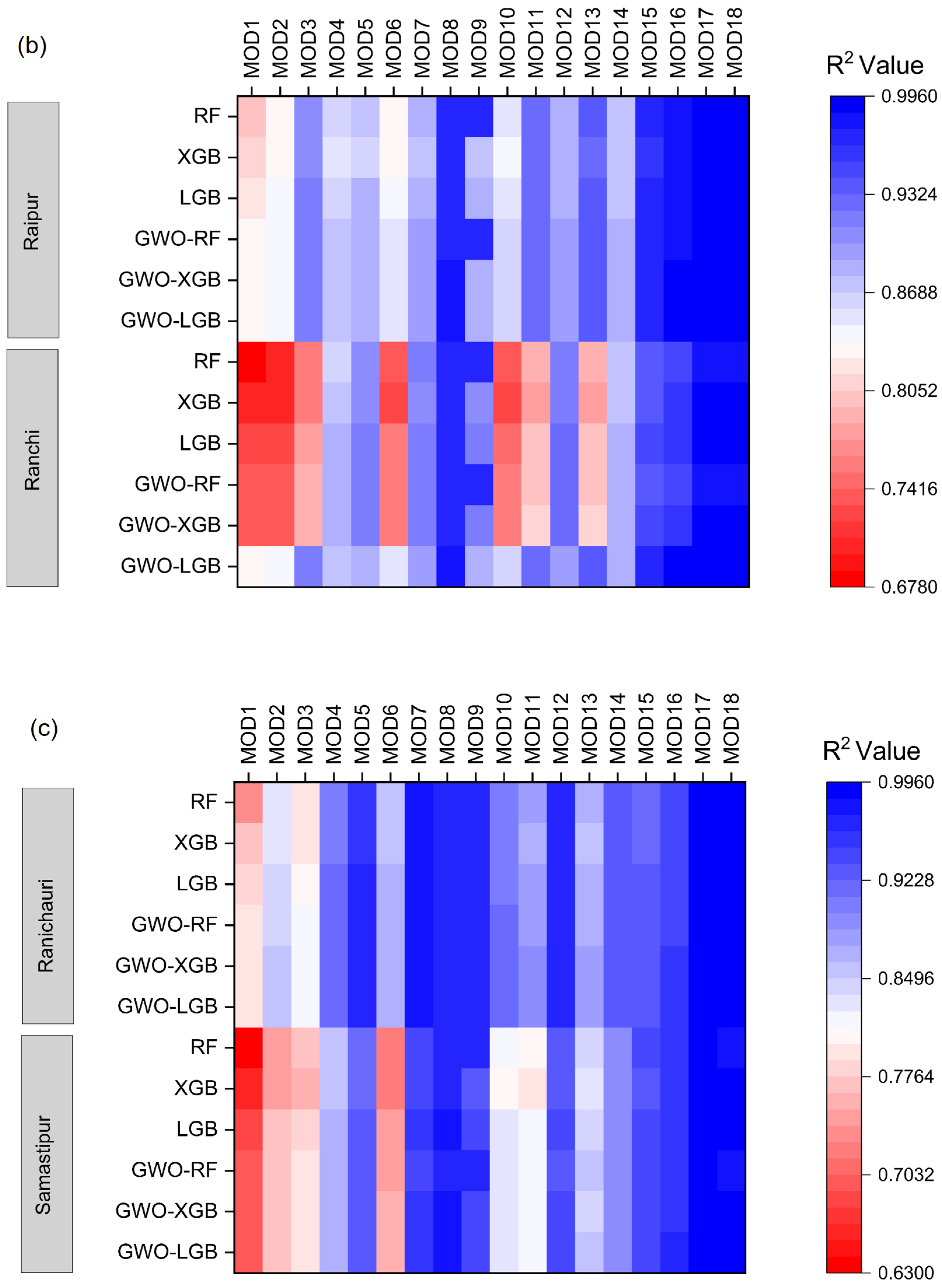
RMSE (mm/day) at sub-humid locations of all ML models at (a) Faizabad, and Jabalpur; (b) Raipur, and Ranchi; (c) Ranichauri, and Samastipur.
Figure 6.
RMSE (mm/day) at sub-humid locations of all ML models at (a) Faizabad, and Jabalpur; (b) Raipur, and Ranchi; (c) Ranichauri, and Samastipur.


Figure 7.
R2 values at sub-humid locations of all ML models at (a) Faizabad, and Jabalpur; (b) Raipur, and Ranchi; (c) Ranichauri, and Samastipur.
Figure 7.
R2 values at sub-humid locations of all ML models at (a) Faizabad, and Jabalpur; (b) Raipur, and Ranchi; (c) Ranichauri, and Samastipur.


Table 1.
Details of the locations of the study area.
| S. No. | State | Station | Code | AER | Latitude (N) | Longitude (E) | Altitude (m) |
|---|---|---|---|---|---|---|---|
| 1 | Assam | Jorhat | JHT | Humid | 26°45′ | 94°12′ | 116 |
| 2 | West Bengal | Mohanpur | MHP | Humid | 21°50′ | 87°15′ | 17 |
| 3 | Himachal Pradesh | Palampur | PLP | Humid | 32°07′ | 76°32′ | 1220 |
| 4 | Kerala | Thrissur | TRS | Humid | 10°31′ | 76°13′ | 28 |
| 5 | Uttar Pradesh | Faizabad | FZB | Sub-humid | 26°46′ | 82°08′ | 97 |
| 6 | Madhya Pradesh | Jabalpur | JBP | Sub-humid | 23°11′ | 79°59′ | 412 |
| 7 | Chattisgarh | Raipur | RPR | Sub-humid | 21°15′ | 81°37′ | 290 |
| 8 | Jharkhand | Ranchi | RNI | Sub-humid | 23°20′ | 85°18′ | 651 |
| 9 | Uttarakhand | Ranichauri | RCH | Sub-humid | 30°19′ | 78°24′ | 1800 |
| 10 | Bihar | Samastipur | SMP | Sub-humid | 25°59′ | 85°40′ | 51 |
Table 2.
Formulae for FAO 56 Penman-Monteith and empirical equations used.
| Method | Symbol and Equations | Reference | |
|---|---|---|---|
| Target for the Models | |||
| FAO-56 Penman-Monteith | (1) | [40] | |
| Mass Transfer based | |||
| Albrecht (ALB) | ETALB = where | (2) | [6] |
| Mahringer (MAH) | where | (3) | [7] |
| Penman (PEN) | where | (4) | [8,41] |
| Radiation based | |||
| Jensen-Haise (JH) | (5) | [11,42] | |
| Makkink (MAK) | (6) | [43] | |
| McGuinness-Bordne (MGB) | (7) | [12] | |
| Priestly-Taylor (PT) | (8) | [13] | |
| Turc (TUR) | (9) | [14] | |
| Temperature based | |||
| Hargreaves-Samani (HS) | (10) | [16] | |
| Hargreaves-Samani 1 (HS1) | (11) | [17] | |
| Hargreaves-Samani 2 (HS2) | (12) | [17] | |
| Thorththwaite (Modified) (THO) | (13) | [44] | |
| Combination based | |||
| Copais (COP) | (14) | [18] | |
| Valiantzas 1 (VA1) | ETVA1 = | (15) | [19] |
| Valiantzas 2 (VA2) | ETVA2 = | (16) | [19] |
Notes: Units and Description of the parameters unless specified above: ET is the reference evapotranspiration, mm/day; ∆ is the slope of the vapour pressure curve, kPa/°C, Rn is the net radiation at the crop surface in MJ/ m2 day, G is the soil heat flux density in MJ/ m2 day, γ is the psychrometric constant in kPa/°C, es is the saturation vapour pressure, kPa; ea is the actual vapour pressure, kPa; u2 is the wind speed at 2 m above the ground surface, m/s; Tmean is the mean daily air temperature,°C; Rn is the net solar radiation, MJ/m2 day; Rs is the incident shortwave solar radiation flux, MJ/m2/day; Ra is the extra-terrestrial solar radiation, MJ/m2 day; Tmax is the maximum daily air temperature, °C; Tmin is the minimum daily air temperature, °C; N is the maximum possible duration, hrs; RH is the mean daily relative humidity, %; and φ is latitude, Radians.
Table 3.
Data input scenarios.
| Model Index | Input Combinations | Model Index | Input Combinations |
|---|---|---|---|
| 1 | Tmax, Tmin | 10 | Tmax, Tmin, RH, Ra |
| 2 | Tmax, Tmin, RH | 11 | Tmax, Tmin, U2, Ra |
| 3 | Tmax, Tmin, U2 | 12 | Tmax, Tmin, n, Ra |
| 4 | Tmax, Tmin, n | 13 | Tmax, Tmin, RH, U2 |
| 5 | Tmax, Tmin, Rs | 14 | Tmax, Tmin, RH, n |
| 6 | Tmax, Tmin, Ra | 15 | Tmax, Tmin, U2, n |
| 7 | Tmax, Tmin, RH, Rs | 16 | Tmax, Tmin, RH, U2, n |
| 8 | Tmax, Tmin, U2, Rs | 17 | Tmax, Tmin, RH, U2, n, Rs |
| 9 | Tmax, Tmin, n, Rs | 18 | Tmax, Tmin, RH, U2, n, Ra |
Table 4.
Cross-validation stages.
| Cross-Validation | Training | Testing |
|---|---|---|
| V1 | 2005–2020 | 2001–2004 |
| V2 | 2001–2004 and 2009–2020 | 2005–2008 |
| V3 | 2001–2008 and 2013–2020 | 2009–2012 |
| V4 | 2001–2012 and 2017–2020 | 2013–2016 |
| V5 | 2001–2016 | 2017–2020 |
Table 5.
Hyperparameter plane for tuning the parameters using GWO.
| Model | Parameter | Default Value | Hyperparameter Range for Tuning |
|---|---|---|---|
| RF | n_estimators | 100 | Range of 10 to 500, increment by 10 |
| min_samples_leaf | 1 | Range of 1 to 6, increment by 2 | |
| max_depth | None | Range of 2 to 20, increment by 2 and None | |
| XGB | n_estimators | 100 | Range of 10 to 500, increment by 10 |
| learning_rate | 0.3 | [0.05, 0.1, 0.15, 0.3] | |
| max_depth | 6 | Range of 2 to 20, increment by 2 and None | |
| LGB | n_estimators | 100 | Range of 10 to 500, increment by 10 |
| learning_rate | 0.3 | [0.05, 0.1, 0.15, 0.3] | |
| max_depth | 6 | Range of 2 to 20, increment by 2 and None |
Table 6.
Statistical indicators.
| Indicator | Code | Formula | |
|---|---|---|---|
| Root mean square error | RMSE | (18) | |
| Coefficient of determination | R2 | (19) | |
| Mean absolute error | MAE | (20) | |
| Agreement index | d | (21) | |
Notes: N is the total number of test data, Oi and Pi are the actual ET0 by FAO 56 Penman-Monteith and predicted values of the models, respectively.
Table 7.
Ranking of the best-performing empirical models at humid stations.
| Jorhat | Mohanpur | Palampur | Thrissur | |||||
|---|---|---|---|---|---|---|---|---|
| RANK | MODEL | GPI | MODEL | GPI | MODEL | GPI | MODEL | GPI |
| 1 | TUR | 1.467 | MAK | 1.521 | TUR | 1.423 | TUR | 1.439 |
| 2 | PT | 1.390 | TUR | 1.508 | VA2 | 1.292 | VA2 | 1.305 |
| 3 | MAK | 1.276 | PT | 1.330 | JH | 0.863 | PT | 0.818 |
| 4 | VA2 | 1.216 | VA2 | 1.027 | HS | 0.783 | MAK | 0.769 |
| 5 | JH | 0.550 | VA1 | 0.813 | PT | 0.721 | PEN | 0.372 |
| 6 | VA1 | 0.484 | HS | 0.361 | HS2 | 0.663 | JH | 0.154 |
| 7 | HS | −0.265 | HS2 | 0.082 | MAK | 0.613 | ALB | 0.034 |
| 8 | ALB | −0.302 | HS1 | 0.052 | HS1 | 0.467 | HS | 0.028 |
| 9 | COP | −0.370 | THO | 0.032 | THO | −0.233 | MAH | −0.084 |
| 10 | HS2 | −0.488 | JH | −0.092 | MAH | −0.516 | HS2 | −0.111 |
| 11 | HS1 | −0.552 | COP | −0.812 | PEN | −0.517 | COP | −0.171 |
| 12 | THO | −0.579 | ALB | −1.033 | ALB | −0.586 | HS1 | −0.351 |
| 13 | PEN | −0.782 | PEN | −1.173 | COP | −1.071 | VA1 | −0.727 |
| 14 | MAH | −0.807 | MAH | −1.687 | MGB | −1.323 | THO | −0.917 |
| 15 | MGB | −2.238 | MGB | −1.927 | VA1 | −2.577 | MGB | −2.559 |
Table 8.
Ranking of the best-performing empirical models at sub-humid stations.
| Faizabad | Jabalpur | Raipur | Ranchi | Ranichauri | Samastipur | |||||||
|---|---|---|---|---|---|---|---|---|---|---|---|---|
| RANK | MODEL | GPI | MODEL | GPI | MODEL | GPI | MODEL | GPI | MODEL | GPI | MODEL | GPI |
| 1 | TUR | 1.037 | TUR | 1.234 | TUR | 1.117 | TUR | 1.587 | VA2 | 1.487 | TUR | 1.037 |
| 2 | JH | 0.882 | VA2 | 1.014 | VA2 | 0.969 | PT | 1.510 | TUR | 1.468 | JH | 0.882 |
| 3 | VA2 | 0.840 | PT | 0.887 | HS | 0.894 | VA2 | 1.294 | MAK | 1.258 | VA2 | 0.840 |
| 4 | HS | 0.642 | HS | 0.686 | PT | 0.784 | MAK | 1.122 | JH | 1.048 | HS | 0.642 |
| 5 | HS1 | 0.520 | JH | 0.646 | HS1 | 0.722 | JH | 0.347 | PT | 0.932 | HS1 | 0.520 |
| 6 | PT | 0.517 | HS1 | 0.487 | HS2 | 0.705 | HS | 0.311 | HS | 0.875 | PT | 0.517 |
| 7 | HS2 | 0.500 | THO | 0.444 | JH | 0.556 | THO | 0.262 | HS2 | 0.762 | HS2 | 0.500 |
| 8 | THO | 0.390 | HS2 | 0.440 | THO | 0.414 | HS1 | −0.059 | HS1 | 0.544 | THO | 0.390 |
| 9 | COP | 0.119 | MAK | 0.377 | MAK | 0.171 | HS2 | −0.065 | THO | −0.279 | COP | 0.119 |
| 10 | PEN | 0.050 | PEN | −0.150 | PEN | −0.131 | ALB | −0.643 | ALB | −1.032 | PEN | 0.050 |
| 11 | MAK | −0.007 | COP | −0.554 | COP | −0.386 | PEN | −0.661 | MGB | −1.038 | MAK | −0.007 |
| 12 | MGB | −0.737 | MAH | −0.883 | MAH | −1.053 | MAH | −0.729 | MAH | −1.230 | MGB | −0.737 |
| 13 | MAH | −1.148 | MGB | −1.016 | MGB | −1.106 | VA1 | −0.744 | VA1 | −1.552 | MAH | −1.148 |
| 14 | ALB | −1.212 | ALB | −1.501 | ALB | −1.523 | COP | −1.493 | COP | −1.567 | ALB | −1.212 |
| 15 | VA1 | −2.392 | VA1 | −2.110 | VA1 | −2.131 | MGB | −2.041 | PEN | −1.675 | VA1 | −2.392 |
Table 9.
Ranking of the best-performing ML models at humid stations.
| Jorhat | Mohanpur | Palampur | Thrissur | |||||
|---|---|---|---|---|---|---|---|---|
| RANK | MODEL | GPI | MODEL | GPI | MODEL | GPI | MODEL | GPI |
| 1 | XGB17 | 1.889 | XGB17 | 1.941 | LGB18 | 1.952 | LGB18 | 1.199 |
| 2 | XGB18 | 1.753 | LGB17 | 1.939 | LGB17 | 1.893 | LGB17 | 1.187 |
| 3 | LGB17 | 1.717 | LGB18 | 1.721 | XGB18 | 1.777 | XGB17 | 1.159 |
| 4 | LGB18 | 1.716 | XGB18 | 1.691 | XGB17 | 1.755 | XGB18 | 1.118 |
| 5 | RF17 | 0.795 | RF17 | 1.424 | RF18 | 1.658 | RF17 | 0.911 |
| 6 | XGB8 | 0.748 | RF18 | 1.286 | RF17 | 1.501 | RF18 | 0.769 |
| 7 | LGB8 | 0.721 | LGB8 | 0.853 | LGB7 | −0.063 | LGB16 | 0.224 |
| 8 | RF18 | 0.582 | XGB8 | 0.702 | RF7 | −0.146 | LGB8 | 0.130 |
| 9 | RF8 | 0.309 | RF9 | 0.607 | XGB7 | −0.258 | XGB16 | 0.077 |
| 10 | RF9 | 0.304 | RF8 | 0.598 | LGB16 | −0.337 | XGB8 | 0.067 |
| 11 | LGB12 | −0.699 | LGB9 | −1.208 | RF16 | −0.527 | RF16 | −0.008 |
| 12 | LGB9 | −0.726 | LGB12 | −1.369 | XGB16 | −0.628 | RF8 | −0.010 |
| 13 | RF12 | −1.040 | RF12 | −1.439 | LGB8 | −1.070 | RF9 | −0.017 |
| 14 | XGB9 | −1.231 | LGB7 | −1.546 | RF8 | −1.191 | LGB15 | −0.413 |
| 15 | XGB12 | −1.321 | XGB9 | −1.619 | RF9 | −1.212 | RF15 | −0.536 |
| 16 | LGB7 | −1.633 | RF7 | −1.712 | XGB8 | −1.373 | XGB15 | −0.558 |
| 17 | RF7 | −1.806 | XGB12 | −1.815 | LGB12 | −1.684 | LGB7 | −2.499 |
| 18 | XGB7 | −2.079 | XGB7 | −2.053 | XGB12 | −2.048 | XGB7 | −2.801 |
Table 10.
Ranking of the best-performing ML models at sub-humid stations.
| Faizabad | Jabalpur | Raipur | Ranchi | Ranichauri | Samastipur | |||||||
|---|---|---|---|---|---|---|---|---|---|---|---|---|
| RANK | MODEL | GPI | MODEL | GPI | MODEL | GPI | MODEL | GPI | MODEL | GPI | MODEL | GPI |
| 1 | LGB17 | 1.752 | LGB18 | 1.265 | LGB18 | 1.265 | LGB17 | 1.637 | LGB17 | 2.374 | LGB17 | 1.908 |
| 2 | LGB18 | 1.682 | LGB17 | 1.222 | LGB17 | 1.248 | XGB17 | 1.593 | LGB18 | 2.303 | LGB18 | 1.821 |
| 3 | XGB17 | 1.630 | XGB18 | 1.138 | XGB18 | 1.197 | LGB18 | 1.566 | XGB17 | 2.207 | XGB17 | 1.761 |
| 4 | XGB18 | 1.561 | XGB17 | 1.137 | XGB17 | 1.191 | XGB18 | 1.546 | XGB18 | 2.034 | XGB18 | 1.583 |
| 5 | RF17 | 1.373 | RF17 | 0.993 | RF17 | 1.036 | RF17 | 1.147 | RF18 | 1.693 | RF17 | 1.397 |
| 6 | RF18 | 1.321 | RF18 | 0.965 | RF18 | 0.973 | RF18 | 1.065 | RF17 | 1.531 | RF18 | 1.041 |
| 7 | LGB16 | 0.162 | LGB16 | 0.347 | LGB16 | 0.473 | LGB8 | 0.463 | LGB7 | 0.216 | LGB8 | 0.282 |
| 8 | XGB16 | −0.027 | XGB16 | 0.195 | XGB16 | 0.323 | RF8 | 0.321 | RF7 | −0.005 | RF9 | 0.135 |
| 9 | LGB8 | −0.125 | RF16 | 0.112 | RF16 | 0.247 | RF9 | 0.304 | XGB7 | −0.071 | RF8 | 0.128 |
| 10 | RF9 | −0.156 | LGB8 | 0.079 | LGB8 | −0.070 | XGB8 | 0.281 | LGB9 | −1.159 | XGB8 | 0.037 |
| 11 | RF8 | −0.195 | RF8 | 0.016 | RF9 | −0.131 | LGB16 | −0.394 | LGB8 | −1.164 | LGB16 | −0.586 |
| 12 | RF16 | −0.289 | RF9 | 0.015 | RF8 | −0.140 | XGB16 | −0.601 | LGB12 | −1.237 | RF16 | −0.746 |
| 13 | XGB8 | −0.298 | XGB8 | −0.076 | XGB8 | −0.193 | RF16 | −0.749 | RF9 | −1.358 | XGB16 | −0.888 |
| 14 | LGB15 | −1.194 | LGB15 | −0.608 | LGB15 | −0.607 | LGB15 | −1.136 | RF8 | −1.388 | LGB7 | −1.211 |
| 15 | XGB15 | −1.460 | RF15 | −0.769 | RF15 | −0.771 | RF15 | −1.357 | RF12 | −1.416 | RF7 | −1.354 |
| 16 | RF15 | −1.520 | XGB15 | −0.845 | XGB15 | −0.851 | XGB15 | −1.361 | XGB9 | −1.459 | XGB7 | −1.502 |
| 17 | LGB13 | −1.970 | LGB13 | −2.450 | LGB13 | −2.455 | LGB12 | −1.962 | XGB8 | −1.474 | LGB15 | −1.713 |
| 18 | XGB13 | −2.248 | XGB13 | −2.735 | XGB13 | −2.735 | XGB12 | −2.363 | XGB12 | −1.626 | XGB12 | −2.092 |
Table 11.
Ranking of the least-performing ML models at humid stations.
| Jorhat | Mohanpur | Palampur | Thrissur | |||||
|---|---|---|---|---|---|---|---|---|
| RANK | MODEL | GPI | MODEL | GPI | MODEL | GPI | MODEL | GPI |
| 54 | RF1 | −2.139 | RF1 | −2.503 | RF1 | −2.748 | RF1 | −2.429 |
| 53 | XGB1 | −1.541 | XGB1 | −1.401 | XGB1 | −2.185 | XGB1 | −1.862 |
| 52 | LGB1 | −1.099 | RF2 | −1.098 | LGB1 | −1.766 | LGB1 | −1.542 |
| 51 | RF3 | −0.885 | XGB2 | −0.907 | RF3 | −0.781 | RF6 | −1.450 |
| 50 | XGB3 | −0.743 | LGB1 | −0.789 | XGB3 | −0.390 | XGB6 | −1.296 |
| 49 | XGB6 | −0.458 | RF3 | −0.404 | RF6 | −0.249 | LGB6 | −1.054 |
| 48 | LGB3 | −0.405 | LGB2 | −0.208 | XGB6 | −0.071 | RF2 | −0.006 |
| 47 | RF6 | −0.403 | XGB3 | −0.142 | LGB3 | −0.042 | XGB2 | 0.111 |
| 46 | XGB11 | −0.036 | RF6 | 0.032 | LGB6 | 0.410 | XGB10 | 0.332 |
| 45 | RF11 | −0.028 | XGB6 | 0.117 | RF4 | 0.497 | LGB2 | 0.334 |
| 44 | LGB6 | 0.029 | XGB13 | 0.513 | RF2 | 0.607 | RF10 | 0.362 |
| 43 | LGB11 | 0.198 | LGB3 | 0.533 | XGB4 | 0.704 | LGB10 | 0.569 |
| 42 | RF2 | 0.649 | RF13 | 0.728 | XGB11 | 0.733 | RF3 | 1.111 |
| 41 | XGB2 | 0.682 | LGB6 | 0.813 | XGB2 | 0.807 | XGB3 | 1.130 |
| 40 | LGB2 | 1.076 | XGB10 | 0.884 | RF11 | 0.976 | LGB3 | 1.335 |
| 39 | XGB10 | 1.532 | RF10 | 1.141 | LGB4 | 1.110 | XGB13 | 1.372 |
| 38 | RF10 | 1.709 | LGB13 | 1.192 | LGB11 | 1.190 | RF5 | 1.413 |
| 37 | LGB10 | 1.861 | LGB10 | 1.497 | LGB2 | 1.197 | LGB5 | 1.571 |
Table 12.
Ranking of the least-performing ML models at sub-humid stations.
| Faizabad | Jabalpur | Raipur | Ranchi | Ranichauri | Samastipur | |||||||
|---|---|---|---|---|---|---|---|---|---|---|---|---|
| RANK | MODEL | GPI | MODEL | GPI | MODEL | GPI | MODEL | GPI | MODEL | GPI | MODEL | GPI |
| 54 | RF1 | −2.377 | RF1 | −2.344 | RF1 | −2.271 | RF1 | −2.028 | RF1 | −2.560 | RF1 | −2.505 |
| 53 | XGB1 | −1.815 | XGB1 | −1.787 | XGB1 | −1.686 | XGB2 | −1.328 | XGB1 | −1.774 | XGB1 | −1.999 |
| 52 | LGB1 | −0.991 | LGB1 | −1.128 | LGB1 | −0.998 | RF2 | −1.215 | LGB1 | −1.307 | LGB1 | −1.514 |
| 51 | XGB2 | −0.618 | XGB2 | −1.103 | XGB2 | −0.758 | XGB1 | −1.164 | RF3 | −1.065 | RF6 | −0.654 |
| 50 | RF2 | −0.471 | RF2 | −0.919 | RF2 | −0.629 | LGB2 | −0.549 | XGB3 | −1.047 | XGB6 | −0.624 |
| 49 | RF6 | −0.439 | XGB6 | −0.504 | XGB6 | −0.544 | LGB1 | −0.509 | LGB3 | −0.596 | XGB2 | −0.315 |
| 48 | XGB4 | −0.407 | LGB2 | −0.475 | RF6 | −0.524 | XGB10 | −0.480 | XGB2 | −0.131 | RF2 | −0.202 |
| 47 | XGB6 | −0.388 | RF6 | −0.283 | LGB2 | −0.302 | XGB6 | −0.419 | RF2 | −0.075 | LGB6 | −0.161 |
| 46 | RF4 | −0.171 | LGB6 | 0.106 | XGB10 | −0.096 | RF6 | −0.268 | LGB2 | 0.287 | XGB3 | 0.053 |
| 45 | LGB2 | −0.021 | XGB10 | 0.132 | LGB6 | 0.072 | RF10 | −0.097 | XGB6 | 0.497 | LGB2 | 0.172 |
| 44 | LGB6 | 0.068 | RF10 | 0.479 | RF10 | 0.333 | LGB10 | 0.354 | RF6 | 0.560 | RF3 | 0.224 |
| 43 | LGB4 | 0.357 | LGB10 | 0.601 | XGB4 | 0.449 | LGB6 | 0.419 | XGB13 | 0.641 | LGB3 | 0.523 |
| 42 | XGB14 | 0.792 | XGB4 | 0.842 | LGB10 | 0.615 | XGB3 | 0.629 | RF13 | 0.790 | XGB11 | 0.790 |
| 41 | RF14 | 1.069 | RF4 | 0.912 | RF4 | 0.713 | RF3 | 0.677 | LGB6 | 0.843 | RF11 | 1.055 |
| 40 | XGB10 | 1.185 | LGB4 | 1.255 | LGB4 | 1.088 | XGB13 | 1.228 | LGB13 | 1.026 | XGB10 | 1.115 |
| 39 | LGB14 | 1.263 | XGB3 | 1.277 | XGB5 | 1.178 | LGB3 | 1.306 | XGB11 | 1.104 | LGB11 | 1.232 |
| 38 | RF5 | 1.339 | RF3 | 1.285 | RF5 | 1.632 | RF13 | 1.473 | RF11 | 1.366 | RF10 | 1.316 |
| 37 | LGB10 | 1.623 | LGB14 | 1.656 | LGB14 | 1.729 | LGB13 | 1.972 | LGB11 | 1.440 | LGB10 | 1.495 |
Table 13.
Comparison of the empirical models with conventional ML models (Humid).
| Jorhat | Mohanpur | Palampur | Thrissur | ||||||
|---|---|---|---|---|---|---|---|---|---|
| Inputs used | RANK | MODEL | GPI | MODEL | GPI | MODEL | GPI | MODEL | GPI |
| Tmax, Tmin, RH, U2 | 1 | LGB13 | 1.708 | LGB13 | 1.696 | LGB13 | 1.908 | LGB13 | 1.802 |
| 2 | RF13 | 1.576 | RF13 | 1.639 | RF13 | 1.844 | RF13 | 1.690 | |
| 3 | XGB13 | 1.561 | XGB13 | 1.612 | XGB13 | 1.808 | XGB13 | 1.639 | |
| 4 | ALB | −0.988 | ALB | −1.315 | MAH | −1.786 | PEN | −1.195 | |
| 5 | PEN | −1.823 | PEN | −1.501 | PEN | −1.849 | ALB | −1.842 | |
| 6 | MAH | −2.034 | MAH | −2.132 | ALB | −1.925 | MAH | −2.093 | |
| Tmax, Tmin, Rs | 1 | LGB5 | 0.824 | LGB5 | 0.982 | LGB5 | 1.037 | LGB5 | 0.942 |
| 2 | RF5 | 0.792 | RF5 | 0.974 | XGB5 | 0.990 | RF5 | 0.907 | |
| 3 | XGB5 | 0.786 | XGB5 | 0.966 | RF5 | 0.975 | XGB5 | 0.902 | |
| 4 | PT | 0.560 | MAK | 0.501 | JH | 0.178 | PT | 0.337 | |
| 5 | MAK | 0.410 | PT | 0.435 | PT | −0.001 | MAK | 0.293 | |
| 6 | JH | −0.246 | JH | −0.870 | MAK | −0.216 | JH | −0.323 | |
| 7 | MGB | −3.126 | MGB | −2.988 | MGB | −2.963 | MGB | −3.058 | |
| Tmax, Tmin, Ra | 1 | LGB6 | 2.110 | LGB6 | 1.864 | LGB6 | 1.306 | LGB6 | 1.678 |
| 2 | RF6 | 1.483 | XGB6 | 1.660 | XGB6 | 1.071 | XGB6 | 1.525 | |
| 3 | XGB6 | 1.369 | RF6 | 1.635 | RF6 | 0.984 | RF6 | 1.436 | |
| 4 | HS | −0.676 | HS | −0.685 | HS | 0.352 | HS | −0.212 | |
| 5 | HS1 | −1.245 | HS2 | −1.400 | HS2 | −0.163 | HS2 | −0.746 | |
| 6 | HS2 | −1.328 | HS1 | −1.416 | HS1 | −0.856 | HS1 | −1.398 | |
| 7 | THO | −1.713 | THO | −1.657 | THO | −2.694 | THO | −2.282 | |
| Tmax, Tmin, RH, Rs | 1 | LGB7 | 1.272 | LGB7 | 1.219 | LGB7 | 1.177 | LGB7 | 1.235 |
| 2 | RF7 | 1.230 | RF7 | 1.206 | RF7 | 1.168 | RF7 | 1.227 | |
| 3 | XGB7 | 1.162 | XGB7 | 1.180 | XGB7 | 1.156 | XGB7 | 1.199 | |
| 4 | TUR | 0.731 | TUR | 0.361 | TUR | 0.880 | TUR | 0.854 | |
| 5 | VA2 | 0.177 | VA2 | −0.368 | VA2 | 0.760 | VA2 | 0.638 | |
| 6 | VA1 | −1.113 | VA1 | −0.455 | COP | −1.439 | COP | −1.656 | |
| 7 | COP | −2.728 | COP | −2.781 | VA1 | −2.823 | VA1 | −2.643 | |
Table 14.
Comparison of the empirical models with conventional ML models (Sub-humid).
| Faizabad | Jabalpur | Raipur | Ranchi | Ranichauri | Samastipur | ||||||||
|---|---|---|---|---|---|---|---|---|---|---|---|---|---|
| Inputs used | RANK | MODEL | GPI | MODEL | GPI | MODEL | GPI | MODEL | GPI | MODEL | GPI | MODEL | GPI |
| Tmax, Tmin, RH, U2 | 1 | LGB13 | 1.535 | LGB13 | 1.502 | LGB13 | 1.523 | LGB13 | 1.860 | LGB13 | 1.763 | LGB13 | 1.425 |
| 2 | RF13 | 1.517 | RF13 | 1.465 | RF13 | 1.498 | RF13 | 1.746 | RF13 | 1.705 | RF13 | 1.404 | |
| 3 | XGB13 | 1.507 | XGB13 | 1.458 | XGB13 | 1.487 | XGB13 | 1.690 | XGB13 | 1.668 | XGB13 | 1.317 | |
| 4 | PEN | −0.909 | PEN | −0.982 | PEN | −0.970 | PEN | −1.665 | ALB | −1.308 | PEN | −0.827 | |
| 5 | MAH | −1.687 | MAH | −1.336 | MAH | −1.433 | ALB | −1.720 | MAH | −1.590 | MAH | −1.464 | |
| 6 | ALB | −1.962 | ALB | −2.107 | ALB | −2.104 | MAH | −1.910 | PEN | −2.237 | ALB | −1.854 | |
| Tmax, Tmin, Rs | 1 | LGB5 | 1.303 | LGB5 | 1.210 | LGB5 | 1.280 | LGB5 | 0.960 | LGB5 | 0.913 | LGB5 | 1.536 |
| 2 | RF5 | 1.211 | RF5 | 1.175 | RF5 | 1.253 | RF5 | 0.924 | RF5 | 0.882 | RF5 | 1.496 | |
| 3 | XGB5 | 1.196 | XGB5 | 1.156 | XGB5 | 1.189 | XGB5 | 0.918 | XGB5 | 0.881 | XGB5 | 1.490 | |
| 4 | JH | 0.465 | PT | 0.064 | PT | 0.002 | PT | 0.582 | MAK | 0.424 | JH | −0.090 | |
| 5 | PT | −0.483 | JH | −0.131 | JH | −0.141 | MAK | 0.159 | JH | 0.058 | PT | −0.749 | |
| 6 | MAK | −1.162 | MAK | −0.684 | MAK | −0.862 | JH | −0.503 | PT | −0.071 | MAK | −1.365 | |
| 7 | MGB | −2.530 | MGB | −2.790 | MGB | −2.720 | MGB | −3.040 | MGB | −3.087 | MGB | −2.318 | |
| Tmax, Tmin, Ra | 1 | LGB6 | 1.866 | LGB6 | 1.741 | LGB6 | 1.716 | LGB6 | 1.517 | LGB6 | 1.138 | LGB6 | 1.917 |
| 2 | XGB6 | 1.615 | RF6 | 1.613 | RF6 | 1.531 | RF6 | 1.280 | RF6 | 0.992 | XGB6 | 1.559 | |
| 3 | RF6 | 1.593 | XGB6 | 1.539 | XGB6 | 1.523 | XGB6 | 1.226 | XGB6 | 0.960 | RF6 | 1.535 | |
| 4 | HS | −0.667 | HS | −0.636 | HS | −0.367 | HS | −0.514 | HS | 0.522 | HS | −0.772 | |
| 5 | HS1 | −1.265 | THO | −1.342 | HS1 | −1.161 | THO | −0.632 | HS2 | 0.036 | HS1 | −1.147 | |
| 6 | HS2 | −1.365 | HS1 | −1.386 | HS2 | −1.201 | HS1 | −1.429 | HS1 | −0.785 | HS2 | −1.246 | |
| 7 | THO | −1.777 | HS2 | −1.530 | THO | −2.040 | HS2 | −1.448 | THO | −2.862 | THO | −1.845 | |
| Tmax, Tmin, RH, Rs | 1 | LGB7 | 0.946 | LGB7 | 1.071 | RF7 | 1.063 | LGB7 | 1.156 | LGB7 | 0.979 | LGB7 | 1.141 |
| 2 | RF7 | 0.938 | RF7 | 1.063 | LGB7 | 1.061 | RF7 | 1.132 | RF7 | 0.966 | RF7 | 1.131 | |
| 3 | XGB7 | 0.875 | XGB7 | 1.039 | XGB7 | 1.021 | XGB7 | 1.103 | XGB7 | 0.962 | XGB7 | 1.120 | |
| 4 | TUR | 0.477 | TUR | 0.675 | TUR | 0.544 | TUR | 0.724 | VA2 | 0.794 | TUR | 0.143 | |
| 5 | VA2 | 0.275 | VA2 | 0.436 | VA2 | 0.387 | VA2 | 0.441 | TUR | 0.776 | VA2 | −0.028 | |
| 6 | COP | −0.457 | COP | −1.354 | COP | −1.139 | VA1 | −1.982 | COP | −2.163 | COP | −0.648 | |
| 7 | VA1 | −3.054 | VA1 | −2.929 | VA1 | −2.937 | COP | −2.574 | VA1 | −2.312 | VA1 | −2.859 | |
Table 15.
Ranking of the best-performing GWO–ML models at humid stations.
| Jorhat | Mohanpur | Palampur | Thrissur | |||||
|---|---|---|---|---|---|---|---|---|
| RANK | MODEL | GPI | MODEL | GPI | MODEL | GPI | MODEL | GPI |
| 1 | GWOXGB17 | 2.175 | GWOXGB17 | 2.176 | GWOXGB18 | 2.078 | GWOXGB18 | 1.376 |
| 2 | GWOXGB18 | 2.134 | GWOXGB18 | 2.072 | GWOLGB18 | 2.078 | GWOLGB18 | 1.360 |
| 3 | GWOLGB18 | 1.843 | GWOLGB17 | 2.052 | GWOXGB17 | 2.038 | GWOXGB17 | 1.287 |
| 4 | GWOLGB17 | 1.747 | GWOLGB18 | 1.798 | GWOLGB17 | 2.030 | GWOLGB17 | 1.271 |
| 5 | GWOXGB8 | 0.854 | GWORF17 | 1.209 | GWORF18 | 1.621 | GWORF17 | 0.820 |
| 6 | GWORF17 | 0.530 | GWORF18 | 1.079 | GWORF17 | 1.466 | GWORF18 | 0.687 |
| 7 | GWOLGB8 | 0.469 | GWOXGB8 | 0.812 | GWOXGB7 | −0.197 | GWOLGB16 | 0.220 |
| 8 | GWORF18 | 0.313 | GWOLGB8 | 0.731 | GWOLGB7 | −0.207 | GWOXGB16 | 0.183 |
| 9 | GWORF8 | 0.041 | GWORF8 | 0.421 | GWORF7 | −0.252 | GWOLGB8 | 0.101 |
| 10 | GWORF9 | −0.167 | GWORF9 | 0.357 | GWOLGB16 | −0.457 | GWOXGB8 | 0.059 |
| 11 | GWOLGB12 | −0.835 | GWOLGB9 | −1.312 | GWOXGB16 | −0.468 | GWORF16 | −0.103 |
| 12 | GWOLGB9 | −0.886 | GWOXGB9 | −1.368 | GWORF16 | −0.705 | GWORF8 | −0.123 |
| 13 | GWOXGB9 | −0.912 | GWOLGB12 | −1.496 | GWOLGB8 | −1.258 | GWORF9 | −0.203 |
| 14 | GWORF12 | −0.971 | GWORF12 | −1.599 | GWORF8 | −1.295 | GWOXGB15 | −0.513 |
| 15 | GWOXGB12 | −0.983 | GWOLGB7 | −1.673 | GWORF9 | −1.318 | GWOLGB15 | −0.538 |
| 16 | GWOLGB7 | −1.765 | GWOXGB12 | −1.726 | GWOXGB8 | −1.372 | GWORF15 | −0.650 |
| 17 | GWOXGB7 | −1.782 | GWOXGB7 | −1.749 | GWOLGB12 | −1.861 | GWOLGB7 | −2.610 |
| 18 | GWORF7 | −1.807 | GWORF7 | −1.786 | GWOXGB12 | −1.922 | GWOXGB7 | −2.624 |
Table 16.
Ranking of the best-performing GWO–ML models at sub-humid stations.
| Faizabad | Jabalpur | Raipur | Ranchi | Ranichauri | Samastipur | |||||||
|---|---|---|---|---|---|---|---|---|---|---|---|---|
| RANK | MODEL | GPI | MODEL | GPI | MODEL | GPI | MODEL | GPI | MODEL | GPI | MODEL | GPI |
| 1 | GWOXGB17 | 1.865 | GWOLGB18 | 1.366 | GWOXGB17 | 1.412 | GWOXGB18 | 1.856 | GWOLGB17 | 2.504 | GWOXGB17 | 1.985 |
| 2 | GWOXGB18 | 1.855 | GWOXGB18 | 1.361 | GWOXGB18 | 1.384 | GWOXGB17 | 1.847 | GWOXGB17 | 2.486 | GWOLGB17 | 1.982 |
| 3 | GWOLGB17 | 1.826 | GWOLGB17 | 1.360 | GWOLGB17 | 1.332 | GWOLGB17 | 1.747 | GWOLGB18 | 2.476 | GWOXGB18 | 1.883 |
| 4 | GWOLGB18 | 1.759 | GWOXGB17 | 1.350 | GWOLGB18 | 1.310 | GWOLGB18 | 1.696 | GWOXGB18 | 2.439 | GWOLGB18 | 1.868 |
| 5 | GWORF17 | 1.207 | GWORF17 | 0.900 | GWORF17 | 0.929 | GWORF17 | 0.996 | GWORF18 | 1.547 | GWORF17 | 1.286 |
| 6 | GWORF18 | 1.160 | GWORF18 | 0.877 | GWORF18 | 0.866 | GWORF18 | 0.947 | GWORF17 | 1.393 | GWORF18 | 0.985 |
| 7 | GWOLGB16 | 0.215 | GWOLGB16 | 0.378 | GWOXGB16 | 0.519 | GWOXGB8 | 0.348 | GWOLGB7 | 0.060 | GWOLGB8 | 0.186 |
| 8 | GWOXGB16 | 0.176 | GWOXGB16 | 0.358 | GWOLGB16 | 0.483 | GWOLGB8 | 0.321 | GWOXGB7 | 0.054 | GWOXGB8 | 0.122 |
| 9 | GWOXGB8 | −0.214 | GWORF16 | 0.007 | GWORF16 | 0.149 | GWORF8 | 0.166 | GWORF7 | −0.176 | GWORF8 | 0.011 |
| 10 | GWOLGB8 | −0.255 | GWOXGB8 | −0.009 | GWOLGB8 | −0.113 | GWORF9 | 0.063 | GWOLGB8 | −1.359 | GWORF9 | 0.004 |
| 11 | GWORF8 | −0.359 | GWOLGB8 | −0.013 | GWOXGB8 | −0.142 | GWOXGB16 | −0.338 | GWOXGB8 | −1.365 | GWOLGB16 | −0.653 |
| 12 | GWORF9 | −0.376 | GWORF8 | −0.092 | GWORF8 | −0.259 | GWOLGB16 | −0.423 | GWOLGB9 | −1.369 | GWOXGB16 | −0.762 |
| 13 | GWORF16 | −0.447 | GWORF9 | −0.201 | GWORF9 | −0.363 | GWORF16 | −0.904 | GWOLGB12 | −1.399 | GWORF16 | −0.894 |
| 14 | GWOXGB15 | −1.269 | GWOXGB15 | −0.724 | GWOXGB15 | −0.730 | GWOXGB15 | −1.253 | GWOXGB9 | −1.422 | GWOXGB7 | −1.330 |
| 15 | GWOLGB15 | −1.325 | GWOLGB15 | −0.764 | GWOLGB15 | −0.762 | GWOLGB15 | −1.304 | GWOXGB12 | −1.455 | GWOLGB7 | −1.357 |
| 16 | GWORF15 | −1.679 | GWORF15 | −0.898 | GWORF15 | −0.903 | GWORF15 | −1.488 | GWORF9 | −1.457 | GWORF7 | −1.475 |
| 17 | GWOXGB13 | −2.011 | GWOLGB13 | −2.625 | GWOXGB13 | −2.522 | GWOLGB12 | −2.131 | GWORF12 | −1.464 | GWOLGB15 | −1.837 |
| 18 | GWOLGB13 | −2.128 | GWOXGB13 | −2.630 | GWOLGB13 | −2.588 | GWOXGB12 | −2.144 | GWORF8 | −1.496 | GWOXGB9 | −2.001 |
Table 17.
Ranking of the least-performing GWO–ML models at humid stations.
| Jorhat | Mohanpur | Palampur | Thrissur | |||||
|---|---|---|---|---|---|---|---|---|
| RANK | MODEL | GPI | MODEL | GPI | MODEL | GPI | MODEL | GPI |
| 54 | GWORF1 | −1.832 | GWOXGB1 | −2.195 | GWOXGB1 | −2.715 | GWOXGB1 | −2.220 |
| 53 | GWOLGB1 | −1.798 | GWOLGB1 | −2.163 | GWOLGB1 | −2.690 | GWORF1 | −2.217 |
| 52 | GWOXGB1 | −1.789 | GWORF1 | −2.158 | GWORF1 | −2.666 | GWOLGB1 | −2.183 |
| 51 | GWOLGB3 | −0.965 | GWORF2 | −1.330 | GWOXGB3 | −0.542 | GWORF6 | −1.687 |
| 50 | GWORF3 | −0.944 | GWOLGB2 | −1.314 | GWOLGB3 | −0.523 | GWOLGB6 | −1.648 |
| 49 | GWOXGB3 | −0.802 | GWOXGB2 | −1.142 | GWORF3 | −0.513 | GWOXGB6 | −1.584 |
| 48 | GWORF6 | −0.413 | GWORF3 | −0.257 | GWORF6 | −0.002 | GWORF2 | 0.139 |
| 47 | GWOXGB6 | −0.361 | GWOXGB3 | 0.095 | GWOXGB6 | 0.044 | GWOLGB2 | 0.172 |
| 46 | GWOLGB6 | −0.339 | GWOLGB3 | 0.159 | GWOLGB6 | 0.131 | GWOXGB2 | 0.180 |
| 45 | GWORF11 | −0.271 | GWORF6 | 0.487 | GWORF4 | 0.922 | GWORF10 | 0.422 |
| 44 | GWOLGB11 | −0.189 | GWOLGB6 | 0.576 | GWOXGB4 | 0.924 | GWOLGB10 | 0.475 |
| 43 | GWOXGB11 | 0.065 | GWOXGB6 | 0.600 | GWOXGB11 | 0.953 | GWOXGB10 | 0.490 |
| 42 | GWORF2 | 1.016 | GWORF13 | 0.955 | GWOLGB4 | 0.957 | GWORF3 | 1.447 |
| 41 | GWOLGB2 | 1.072 | GWOLGB13 | 1.301 | GWORF11 | 1.066 | GWOLGB3 | 1.495 |
| 40 | GWOXGB2 | 1.139 | GWOXGB13 | 1.362 | GWOLGB11 | 1.070 | GWOXGB3 | 1.503 |
| 39 | GWORF10 | 2.119 | GWORF10 | 1.560 | GWORF2 | 1.108 | GWORF11 | 1.711 |
| 38 | GWOLGB10 | 2.134 | GWOLGB10 | 1.679 | GWOXGB2 | 1.234 | GWOXGB13 | 1.727 |
| 37 | GWOXGB10 | 2.157 | GWOXGB11 | 1.786 | GWOLGB2 | 1.241 | GWOLGB13 | 1.777 |
Table 18.
Ranking of the least-performing GWO–ML models at sub-humid stations.
| Faizabad | Jabalpur | Raipur | Ranchi | Ranichauri | Samastipur | |||||||
|---|---|---|---|---|---|---|---|---|---|---|---|---|
| RANK | MODEL | GPI | MODEL | GPI | MODEL | GPI | MODEL | GPI | MODEL | GPI | MODEL | GPI |
| 54 | GWOXGB1 | −2.067 | GWOXGB1 | −2.069 | GWOXGB1 | −2.052 | GWOXGB2 | −1.696 | GWOLGB1 | −2.296 | GWOLGB1 | −2.328 |
| 53 | GWOLGB1 | −2.059 | GWORF1 | −2.025 | GWOLGB1 | −2.029 | GWOLGB2 | −1.618 | GWORF1 | −2.272 | GWORF1 | −2.322 |
| 52 | GWORF1 | −1.942 | GWOLGB1 | −2.018 | GWORF1 | −1.977 | GWORF2 | −1.599 | GWOXGB1 | −2.257 | GWOXGB1 | −2.276 |
| 51 | GWORF6 | −0.563 | GWORF2 | −1.151 | GWOXGB2 | −0.901 | GWOXGB1 | −1.542 | GWORF3 | −1.348 | GWORF6 | −0.666 |
| 50 | GWOLGB2 | −0.460 | GWOXGB2 | −1.084 | GWORF2 | −0.900 | GWORF1 | −1.535 | GWOLGB3 | −1.296 | GWOLGB6 | −0.583 |
| 49 | GWOLGB6 | −0.404 | GWOLGB2 | −1.063 | GWOLGB2 | −0.853 | GWOLGB1 | −1.535 | GWOXGB3 | −1.218 | GWOXGB6 | −0.552 |
| 48 | GWOXGB2 | −0.402 | GWOXGB6 | −0.375 | GWOLGB6 | −0.579 | GWORF10 | −0.354 | GWORF2 | 0.031 | GWOXGB2 | −0.230 |
| 47 | GWOXGB6 | −0.373 | GWORF6 | −0.300 | GWOXGB6 | −0.548 | GWORF6 | −0.304 | GWOXGB2 | 0.032 | GWORF2 | −0.195 |
| 46 | GWORF2 | −0.252 | GWOLGB6 | −0.273 | GWORF6 | −0.514 | GWOXGB10 | −0.148 | GWOLGB2 | 0.046 | GWOLGB2 | −0.165 |
| 45 | GWORF4 | −0.238 | GWOXGB10 | 0.356 | GWOXGB10 | 0.422 | GWOLGB10 | −0.106 | GWORF6 | 0.776 | GWOXGB3 | 0.321 |
| 44 | GWOXGB4 | −0.143 | GWORF10 | 0.462 | GWORF10 | 0.429 | GWOXGB6 | −0.023 | GWOLGB6 | 0.790 | GWOLGB3 | 0.337 |
| 43 | GWOLGB4 | −0.139 | GWOLGB10 | 0.503 | GWOLGB10 | 0.534 | GWOLGB6 | 0.035 | GWOXGB6 | 0.799 | GWORF3 | 0.368 |
| 42 | GWOXGB14 | 1.105 | GWORF4 | 1.126 | GWORF4 | 1.036 | GWORF3 | 1.161 | GWORF13 | 0.956 | GWORF11 | 1.073 |
| 41 | GWOLGB14 | 1.180 | GWOXGB4 | 1.265 | GWOLGB4 | 1.083 | GWOXGB3 | 1.365 | GWOLGB13 | 1.136 | GWOXGB11 | 1.127 |
| 40 | GWORF14 | 1.239 | GWOLGB4 | 1.286 | GWOXGB4 | 1.108 | GWOLGB3 | 1.404 | GWOXGB13 | 1.143 | GWOLGB11 | 1.240 |
| 39 | GWOXGB10 | 1.791 | GWORF14 | 1.757 | GWOXGB14 | 1.904 | GWORF13 | 1.959 | GWORF11 | 1.640 | GWORF10 | 1.534 |
| 38 | GWORF5 | 1.817 | GWOXGB14 | 1.782 | GWORF14 | 1.915 | GWOXGB13 | 2.237 | GWOXGB11 | 1.645 | GWOLGB10 | 1.651 |
| 37 | GWOLGB10 | 1.909 | GWOLGB3 | 1.823 | GWOLGB14 | 1.922 | GWOLGB13 | 2.299 | GWOLGB11 | 1.692 | GWOXGB10 | 1.665 |
Table 19.
Ranking of the best-performing models in conventional and hybrid MLs at humid stations.
| Jorhat | Mohanpur | Palampur | Thrissur | |||||
|---|---|---|---|---|---|---|---|---|
| RANK | MODEL | GPI | MODEL | GPI | MODEL | GPI | MODEL | GPI |
| 1 | GWOXGB17 | 2.031 | GWOXGB17 | 2.077 | GWOXGB18 | 1.953 | GWOXGB18 | 1.302 |
| 2 | GWOXGB18 | 1.995 | GWOXGB18 | 1.982 | GWOLGB18 | 1.953 | GWOLGB18 | 1.288 |
| 3 | GWOLGB18 | 1.740 | GWOLGB17 | 1.964 | GWOXGB17 | 1.916 | GWOXGB17 | 1.222 |
| 4 | GWOLGB17 | 1.656 | GWOLGB18 | 1.732 | GWOLGB17 | 1.909 | GWOLGB17 | 1.207 |
| 5 | XGB17 | 1.538 | XGB17 | 1.635 | LGB18 | 1.810 | LGB18 | 1.062 |
| 6 | XGB18 | 1.419 | LGB17 | 1.633 | LGB17 | 1.754 | LGB17 | 1.051 |
| 7 | LGB17 | 1.388 | LGB18 | 1.439 | XGB18 | 1.642 | XGB17 | 1.025 |
| 8 | LGB18 | 1.388 | XGB18 | 1.413 | XGB17 | 1.621 | XGB18 | 0.987 |
| 9 | GWOXGB8 | 0.869 | GWORF17 | 1.193 | GWORF18 | 1.537 | GWORF17 | 0.799 |
| 10 | GWORF17 | 0.589 | RF17 | 1.176 | RF18 | 1.528 | RF17 | 0.793 |
| 11 | RF17 | 0.579 | GWORF18 | 1.075 | GWORF17 | 1.395 | GWORF18 | 0.679 |
| 12 | GWOLGB8 | 0.533 | RF18 | 1.054 | RF17 | 1.376 | RF18 | 0.661 |
| 13 | XGB8 | 0.533 | GWOXGB8 | 0.829 | GWOXGB7 | −0.110 | GWOLGB16 | 0.252 |
| 14 | LGB8 | 0.510 | GWOLGB8 | 0.755 | GWOLGB7 | −0.119 | GWOXGB16 | 0.220 |
| 15 | GWORF18 | 0.399 | LGB8 | 0.673 | LGB7 | −0.129 | LGB16 | 0.152 |
| 16 | RF18 | 0.392 | XGB8 | 0.540 | GWORF7 | −0.159 | GWOLGB8 | 0.150 |
| 17 | GWORF8 | 0.159 | GWORF8 | 0.473 | RF7 | −0.210 | GWOXGB8 | 0.112 |
| 18 | RF8 | 0.148 | RF9 | 0.454 | XGB7 | −0.318 | LGB8 | 0.063 |
| 19 | RF9 | 0.144 | RF8 | 0.445 | GWOLGB16 | −0.348 | XGB16 | 0.015 |
| 20 | GWORF9 | −0.023 | GWORF9 | 0.414 | GWOXGB16 | −0.358 | XGB8 | 0.005 |
| 21 | GWOLGB12 | −0.607 | GWOLGB9 | −1.103 | LGB16 | −0.393 | GWORF16 | −0.037 |
| 22 | GWOLGB9 | −0.652 | GWOXGB9 | −1.154 | GWORF16 | −0.571 | GWORF8 | −0.050 |
| 23 | GWOXGB9 | −0.675 | LGB9 | −1.169 | RF16 | −0.577 | RF16 | −0.065 |
| 24 | GWORF12 | −0.726 | GWOLGB12 | −1.270 | XGB16 | −0.673 | RF8 | −0.069 |
| 25 | GWOXGB12 | −0.736 | LGB12 | −1.313 | GWOLGB8 | −1.068 | RF9 | −0.075 |
| 26 | LGB12 | −0.739 | GWORF12 | −1.363 | GWORF8 | −1.101 | GWORF9 | −0.123 |
| 27 | LGB9 | −0.762 | RF12 | −1.376 | LGB8 | −1.102 | GWOXGB15 | −0.407 |
| 28 | RF12 | −1.040 | GWOLGB7 | −1.433 | GWORF9 | −1.122 | GWOLGB15 | −0.430 |
| 29 | XGB9 | −1.208 | LGB7 | −1.469 | GWOXGB8 | −1.171 | LGB15 | −0.445 |
| 30 | XGB12 | −1.288 | GWOXGB12 | −1.478 | RF8 | −1.218 | GWORF15 | −0.529 |
| 31 | GWOLGB7 | −1.422 | GWOXGB7 | −1.501 | RF9 | −1.238 | RF15 | −0.561 |
| 32 | GWOXGB7 | −1.436 | GWORF7 | −1.535 | XGB8 | −1.394 | XGB15 | −0.581 |
| 33 | GWORF7 | −1.458 | XGB9 | −1.537 | GWOLGB12 | −1.611 | GWOLGB7 | −2.275 |
| 34 | LGB7 | −1.564 | RF7 | −1.617 | GWOXGB12 | −1.665 | GWOXGB7 | −2.288 |
| 35 | RF7 | −1.717 | XGB12 | −1.712 | LGB12 | −1.694 | LGB7 | −2.413 |
| 36 | XGB7 | −1.958 | XGB7 | −1.923 | XGB12 | −2.047 | XGB7 | −2.698 |
Table 20.
Ranking of the best-performing models in conventional and hybrid MLs at sub-humid stations.
Table 20.
Ranking of the best-performing models in conventional and hybrid MLs at sub-humid stations.
| Faizabad | Jabalpur | Raipur | Ranchi | Ranichauri | Samastipur | |||||||
|---|---|---|---|---|---|---|---|---|---|---|---|---|
| RANK | MODEL | GPI | MODEL | GPI | MODEL | GPI | MODEL | GPI | MODEL | GPI | MODEL | GPI |
| 1 | GWOXGB17 | 1.810 | GWOLGB18 | 1.315 | GWOXGB17 | 1.368 | GWOXGB18 | 1.739 | GWOLGB17 | 2.383 | GWOXGB17 | 1.944 |
| 2 | GWOXGB18 | 1.801 | GWOXGB18 | 1.311 | GWOXGB18 | 1.343 | GWOXGB17 | 1.731 | GWOXGB17 | 2.366 | GWOLGB17 | 1.941 |
| 3 | GWOLGB17 | 1.774 | GWOLGB17 | 1.310 | GWOLGB17 | 1.295 | GWOLGB17 | 1.642 | GWOLGB18 | 2.357 | GWOXGB18 | 1.847 |
| 4 | GWOLGB18 | 1.711 | GWOXGB17 | 1.301 | GWOLGB18 | 1.273 | GWOLGB18 | 1.595 | GWOXGB18 | 2.323 | GWOLGB18 | 1.834 |
| 5 | LGB17 | 1.556 | LGB18 | 1.146 | LGB18 | 1.120 | LGB17 | 1.434 | LGB17 | 2.136 | LGB17 | 1.726 |
| 6 | LGB18 | 1.491 | LGB17 | 1.104 | LGB17 | 1.105 | XGB17 | 1.394 | LGB18 | 2.069 | LGB18 | 1.644 |
| 7 | XGB17 | 1.443 | XGB18 | 1.025 | XGB18 | 1.056 | LGB18 | 1.369 | XGB17 | 1.980 | XGB17 | 1.588 |
| 8 | XGB18 | 1.378 | XGB17 | 1.023 | XGB17 | 1.052 | XGB18 | 1.352 | XGB18 | 1.818 | XGB18 | 1.421 |
| 9 | RF17 | 1.203 | GWORF17 | 0.887 | GWORF17 | 0.921 | RF17 | 0.985 | GWORF18 | 1.505 | GWORF17 | 1.284 |
| 10 | GWORF17 | 1.199 | RF17 | 0.887 | RF17 | 0.907 | GWORF17 | 0.964 | RF18 | 1.499 | RF17 | 1.245 |
| 11 | GWORF18 | 1.155 | GWORF18 | 0.866 | GWORF18 | 0.863 | GWORF18 | 0.921 | GWORF17 | 1.364 | GWORF18 | 1.002 |
| 12 | RF18 | 1.155 | RF18 | 0.860 | RF18 | 0.849 | RF18 | 0.910 | RF17 | 1.347 | RF18 | 0.909 |
| 13 | GWOLGB16 | 0.278 | GWOLGB16 | 0.406 | GWOXGB16 | 0.540 | GWOXGB8 | 0.382 | GWOLGB7 | 0.144 | GWOLGB8 | 0.247 |
| 14 | GWOXGB16 | 0.241 | GWOXGB16 | 0.388 | GWOLGB16 | 0.507 | GWOLGB8 | 0.358 | GWOXGB7 | 0.139 | LGB8 | 0.194 |
| 15 | LGB16 | 0.073 | LGB16 | 0.270 | LGB16 | 0.381 | LGB8 | 0.357 | LGB7 | 0.114 | GWOXGB8 | 0.187 |
| 16 | XGB16 | −0.103 | XGB16 | 0.125 | XGB16 | 0.241 | RF8 | 0.226 | GWORF7 | −0.071 | GWORF8 | 0.083 |
| 17 | GWOXGB8 | −0.119 | GWORF16 | 0.066 | GWORF16 | 0.199 | GWORF8 | 0.219 | RF7 | −0.094 | GWORF9 | 0.077 |
| 18 | GWOLGB8 | −0.157 | GWOXGB8 | 0.053 | RF16 | 0.169 | RF9 | 0.210 | XGB7 | −0.156 | RF9 | 0.055 |
| 19 | LGB8 | −0.196 | GWOLGB8 | 0.050 | GWOLGB8 | −0.042 | XGB8 | 0.189 | GWOLGB8 | −1.152 | RF8 | 0.048 |
| 20 | RF9 | −0.225 | RF16 | 0.045 | GWOXGB8 | −0.069 | GWORF9 | 0.127 | GWOXGB8 | −1.158 | XGB8 | −0.038 |
| 21 | GWORF8 | −0.253 | LGB8 | 0.014 | LGB8 | −0.128 | GWOXGB16 | −0.234 | GWOLGB9 | −1.161 | GWOLGB16 | −0.541 |
| 22 | RF8 | −0.262 | GWORF8 | −0.022 | GWORF8 | −0.175 | GWOLGB16 | −0.310 | LGB9 | −1.178 | LGB16 | −0.627 |
| 23 | GWORF9 | −0.269 | RF8 | −0.047 | RF9 | −0.185 | LGB16 | −0.432 | LGB8 | −1.183 | GWOXGB16 | −0.642 |
| 24 | GWORF16 | −0.335 | RF9 | −0.047 | RF8 | −0.193 | XGB16 | −0.624 | GWOLGB12 | −1.189 | GWORF16 | −0.767 |
| 25 | RF16 | −0.348 | GWORF9 | −0.121 | XGB8 | −0.243 | GWORF16 | −0.741 | GWOXGB9 | −1.210 | RF16 | −0.779 |
| 26 | XGB8 | −0.358 | XGB8 | −0.135 | GWORF9 | −0.272 | RF16 | −0.760 | GWOXGB12 | −1.240 | XGB16 | −0.913 |
| 27 | GWOXGB15 | −1.096 | GWOXGB15 | −0.602 | GWOXGB15 | −0.612 | GWOXGB15 | −1.053 | GWORF9 | −1.242 | GWOXGB7 | −1.176 |
| 28 | GWOLGB15 | −1.148 | GWOLGB15 | −0.638 | LGB15 | −0.631 | GWOLGB15 | −1.098 | GWORF12 | −1.248 | GWOLGB7 | −1.201 |
| 29 | LGB15 | −1.196 | LGB15 | −0.644 | GWOLGB15 | −0.642 | LGB15 | −1.118 | LGB12 | −1.252 | LGB7 | −1.219 |
| 30 | XGB15 | −1.445 | GWORF15 | −0.760 | GWORF15 | −0.771 | GWORF15 | −1.263 | GWORF8 | −1.277 | GWORF7 | −1.312 |
| 31 | GWORF15 | −1.476 | RF15 | −0.798 | RF15 | −0.785 | RF15 | −1.323 | RF9 | −1.366 | RF7 | −1.355 |
| 32 | RF15 | −1.501 | XGB15 | −0.871 | XGB15 | −0.860 | XGB15 | −1.326 | RF8 | −1.393 | XGB7 | −1.495 |
| 33 | GWOXGB13 | −1.783 | GWOLGB13 | −2.335 | GWOXGB13 | −2.261 | GWOLGB12 | −1.831 | RF12 | −1.420 | GWOLGB15 | −1.653 |
| 34 | GWOLGB13 | −1.891 | GWOXGB13 | −2.340 | GWOLGB13 | −2.322 | GWOXGB12 | −1.843 | XGB9 | −1.461 | LGB15 | −1.695 |
| 35 | LGB13 | −1.923 | LGB13 | −2.411 | LGB13 | −2.368 | LGB12 | −1.888 | XGB8 | −1.475 | GWOXGB9 | −1.805 |
| 36 | XGB13 | −2.183 | XGB13 | −2.684 | XGB13 | −2.632 | XGB12 | −2.261 | XGB12 | −1.617 | XGB12 | −2.054 |
Table 21.
Ranking of the least performing models in conventional and hybrid ML at humid stations.
| Jorhat | Mohanpur | Palampur | Thrissur | |||||
|---|---|---|---|---|---|---|---|---|
| RANK | MODEL | GPI | MODEL | GPI | MODEL | GPI | MODEL | GPI |
| 108 | RF1 | −2.443 | RF1 | −2.685 | RF1 | −2.858 | RF1 | −2.488 |
| 107 | XGB1 | −1.829 | XGB1 | −1.645 | XGB1 | −2.313 | XGB1 | −1.934 |
| 106 | LGB1 | −1.374 | RF2 | −1.357 | LGB1 | −1.909 | LGB1 | −1.620 |
| 105 | GWORF1 | −1.158 | XGB2 | −1.176 | GWOXGB1 | −1.811 | GWOXGB1 | −1.543 |
| 104 | RF3 | −1.150 | LGB1 | −1.066 | GWOLGB1 | −1.793 | GWORF1 | −1.541 |
| 103 | GWOLGB1 | −1.134 | GWOXGB1 | −0.891 | GWORF1 | −1.774 | RF6 | −1.530 |
| 102 | GWOXGB1 | −1.128 | GWOLGB1 | −0.875 | RF3 | −0.956 | GWOLGB1 | −1.515 |
| 101 | XGB3 | −1.001 | GWORF1 | −0.871 | XGB3 | −0.578 | XGB6 | −1.380 |
| 100 | XGB6 | −0.703 | RF3 | −0.703 | RF6 | −0.439 | LGB6 | −1.144 |
| 99 | LGB3 | −0.655 | LGB2 | −0.517 | XGB6 | −0.266 | GWORF6 | −1.143 |
| 98 | RF6 | −0.644 | XGB3 | −0.455 | LGB3 | −0.242 | GWOLGB6 | −1.114 |
| 97 | GWOLGB3 | −0.504 | GWORF2 | −0.413 | GWOXGB3 | −0.202 | GWOXGB6 | −1.066 |
| 96 | GWORF3 | −0.488 | GWOLGB2 | −0.405 | GWOLGB3 | −0.188 | RF2 | −0.120 |
| 95 | GWOXGB3 | −0.379 | GWOXGB2 | −0.310 | GWORF3 | −0.180 | XGB2 | −0.006 |
| 94 | XGB11 | −0.264 | RF6 | −0.292 | LGB6 | 0.198 | XGB10 | 0.210 |
| 93 | RF11 | −0.259 | XGB6 | −0.212 | GWORF6 | 0.201 | LGB2 | 0.211 |
| 92 | LGB6 | −0.200 | XGB13 | 0.163 | GWOXGB6 | 0.235 | GWORF2 | 0.221 |
| 91 | GWORF6 | −0.078 | GWORF3 | 0.180 | RF4 | 0.281 | RF10 | 0.239 |
| 90 | GWOXGB6 | −0.040 | LGB3 | 0.182 | GWOLGB6 | 0.299 | GWOLGB2 | 0.246 |
| 89 | LGB11 | −0.025 | RF13 | 0.367 | RF2 | 0.386 | GWOXGB2 | 0.252 |
| 88 | GWOLGB6 | −0.024 | GWOXGB3 | 0.374 | XGB4 | 0.481 | GWORF10 | 0.431 |
| 87 | GWORF11 | 0.028 | GWOLGB3 | 0.409 | XGB11 | 0.511 | LGB10 | 0.442 |
| 86 | GWOLGB11 | 0.090 | LGB6 | 0.446 | XGB2 | 0.580 | GWOLGB10 | 0.470 |
| 85 | GWOXGB11 | 0.284 | XGB10 | 0.513 | RF11 | 0.744 | GWOXGB10 | 0.481 |
| 84 | RF2 | 0.450 | GWORF6 | 0.593 | LGB4 | 0.873 | RF3 | 0.971 |
| 83 | XGB2 | 0.484 | GWOLGB6 | 0.640 | GWORF4 | 0.882 | XGB3 | 0.989 |
| 82 | LGB2 | 0.888 | GWOXGB6 | 0.653 | GWOXGB4 | 0.883 | LGB3 | 1.189 |
| 81 | GWORF2 | 1.004 | RF10 | 0.756 | GWOXGB11 | 0.906 | GWORF3 | 1.192 |
| 80 | GWOLGB2 | 1.045 | LGB13 | 0.804 | GWOLGB4 | 0.908 | XGB13 | 1.226 |
| 79 | GWOXGB2 | 1.097 | GWORF13 | 0.848 | LGB11 | 0.952 | GWOLGB3 | 1.228 |
| 78 | XGB10 | 1.359 | GWOLGB13 | 1.038 | LGB2 | 0.957 | GWOXGB3 | 1.234 |
| 77 | RF10 | 1.540 | GWOXGB13 | 1.071 | GWORF11 | 0.990 | RF5 | 1.269 |
| 76 | LGB10 | 1.695 | LGB10 | 1.092 | GWOLGB11 | 0.993 | GWORF11 | 1.387 |
| 75 | GWORF10 | 1.826 | GWORF10 | 1.183 | GWORF2 | 1.019 | GWOXGB13 | 1.398 |
| 74 | GWOLGB10 | 1.837 | GWOLGB10 | 1.250 | GWOXGB2 | 1.113 | LGB5 | 1.423 |
| 73 | GWOXGB10 | 1.854 | GWOXGB11 | 1.312 | GWOLGB2 | 1.118 | GWOLGB13 | 1.435 |
Table 22.
Ranking of the least-performing models in conventional and hybrid MLs at sub-humid stations.
Table 22.
Ranking of the least-performing models in conventional and hybrid MLs at sub-humid stations.
| Faizabad | Jabalpur | Raipur | Ranchi | Ranichauri | Samastipur | |||||||
|---|---|---|---|---|---|---|---|---|---|---|---|---|
| RANK | MODEL | GPI | MODEL | GPI | MODEL | GPI | MODEL | GPI | MODEL | GPI | MODEL | GPI |
| 108 | RF1 | −2.488 | RF1 | −2.511 | RF1 | −2.473 | RF1 | −2.276 | RF1 | −2.703 | RF1 | −2.620 |
| 107 | XGB1 | −1.954 | XGB1 | −1.969 | XGB1 | −1.909 | XGB2 | −1.606 | XGB1 | −1.931 | XGB1 | −2.127 |
| 106 | LGB1 | −1.173 | LGB1 | −1.330 | LGB1 | −1.246 | RF2 | −1.498 | LGB1 | −1.471 | LGB1 | −1.656 |
| 105 | GWOXGB1 | −1.140 | XGB2 | −1.304 | GWOXGB1 | −1.036 | XGB1 | −1.449 | GWOLGB1 | −1.322 | GWOLGB1 | −1.492 |
| 104 | GWOLGB1 | −1.135 | RF2 | −1.126 | GWOLGB1 | −1.020 | LGB2 | −0.861 | GWORF1 | −1.305 | GWORF1 | −1.487 |
| 103 | GWORF1 | −1.058 | GWOXGB1 | −1.119 | XGB2 | −1.013 | LGB1 | −0.823 | GWOXGB1 | −1.295 | GWOXGB1 | −1.454 |
| 102 | XGB2 | −0.819 | GWORF1 | −1.090 | GWORF1 | −0.986 | XGB10 | −0.793 | RF3 | −1.233 | RF6 | −0.818 |
| 101 | RF2 | −0.679 | GWOLGB1 | −1.086 | RF2 | −0.889 | XGB6 | −0.735 | XGB3 | −1.215 | XGB6 | −0.789 |
| 100 | RF6 | −0.648 | XGB6 | −0.719 | XGB6 | −0.806 | GWOXGB2 | −0.690 | LGB3 | −0.772 | XGB2 | −0.488 |
| 99 | XGB4 | −0.618 | LGB2 | −0.695 | RF6 | −0.787 | GWOLGB2 | −0.643 | GWORF3 | −0.698 | RF2 | −0.379 |
| 98 | XGB6 | −0.599 | GWORF2 | −0.520 | LGB2 | −0.574 | GWORF2 | −0.631 | GWOLGB3 | −0.665 | LGB6 | −0.339 |
| 97 | RF4 | −0.394 | RF6 | −0.504 | XGB10 | −0.372 | GWOXGB1 | −0.597 | GWOXGB3 | −0.614 | GWORF6 | −0.293 |
| 96 | LGB2 | −0.253 | GWOXGB2 | −0.477 | GWOXGB2 | −0.297 | GWOLGB1 | −0.593 | XGB2 | −0.313 | GWOLGB6 | −0.234 |
| 95 | LGB6 | −0.167 | GWOLGB2 | −0.463 | GWORF2 | −0.296 | GWORF1 | −0.593 | RF2 | −0.258 | GWOXGB6 | −0.212 |
| 94 | GWORF6 | −0.139 | LGB6 | −0.127 | GWOLGB2 | −0.266 | RF6 | −0.591 | LGB2 | 0.098 | XGB3 | −0.131 |
| 93 | GWOLGB2 | −0.075 | XGB10 | −0.100 | LGB6 | −0.212 | RF10 | −0.427 | GWOXGB2 | 0.203 | LGB2 | −0.016 |
| 92 | GWOXGB2 | −0.036 | GWOXGB6 | −0.009 | GWOLGB6 | −0.088 | LGB10 | 0.005 | GWORF2 | 0.203 | GWOXGB2 | 0.015 |
| 91 | GWOLGB6 | −0.034 | GWORF6 | 0.040 | GWOXGB6 | −0.068 | LGB6 | 0.066 | GWOLGB2 | 0.213 | RF3 | 0.035 |
| 90 | GWOXGB6 | −0.014 | GWOLGB6 | 0.057 | GWORF6 | −0.044 | GWORF10 | 0.121 | XGB6 | 0.304 | GWORF2 | 0.040 |
| 89 | GWORF2 | 0.063 | RF10 | 0.236 | RF10 | 0.040 | GWORF6 | 0.151 | RF6 | 0.366 | GWOLGB2 | 0.062 |
| 88 | GWORF4 | 0.074 | LGB10 | 0.354 | XGB4 | 0.152 | GWOXGB10 | 0.246 | XGB13 | 0.445 | LGB3 | 0.326 |
| 87 | LGB4 | 0.106 | GWOXGB10 | 0.468 | LGB10 | 0.313 | XGB3 | 0.267 | RF13 | 0.592 | GWOXGB3 | 0.412 |
| 86 | GWOXGB4 | 0.137 | GWORF10 | 0.536 | RF4 | 0.405 | GWOLGB10 | 0.271 | LGB6 | 0.645 | GWOLGB3 | 0.423 |
| 85 | GWOLGB4 | 0.139 | GWOLGB10 | 0.563 | GWOXGB10 | 0.556 | RF3 | 0.313 | GWORF6 | 0.696 | GWORF3 | 0.446 |
| 84 | XGB14 | 0.520 | XGB4 | 0.585 | GWORF10 | 0.559 | GWOXGB6 | 0.321 | GWOLGB6 | 0.706 | XGB11 | 0.586 |
| 83 | RF14 | 0.783 | RF4 | 0.652 | GWOLGB10 | 0.626 | GWOLGB6 | 0.356 | GWOXGB6 | 0.711 | RF11 | 0.844 |
| 82 | XGB10 | 0.893 | GWORF4 | 0.964 | LGB4 | 0.767 | XGB13 | 0.840 | GWORF13 | 0.810 | XGB10 | 0.903 |
| 81 | LGB14 | 0.967 | LGB4 | 0.986 | XGB5 | 0.857 | LGB3 | 0.915 | LGB13 | 0.825 | GWORF11 | 0.954 |
| 80 | GWOXGB14 | 0.967 | XGB3 | 1.006 | GWORF4 | 0.942 | GWORF3 | 1.036 | XGB11 | 0.902 | GWOXGB11 | 0.993 |
| 79 | GWOLGB14 | 1.017 | RF3 | 1.014 | GWOLGB4 | 0.972 | RF13 | 1.075 | GWOLGB13 | 0.927 | LGB11 | 1.016 |
| 78 | RF5 | 1.039 | GWOXGB4 | 1.055 | GWOXGB4 | 0.986 | GWOXGB3 | 1.159 | GWOXGB13 | 0.932 | GWOLGB11 | 1.074 |
| 77 | GWORF14 | 1.054 | GWOLGB4 | 1.068 | RF5 | 1.293 | GWOLGB3 | 1.183 | RF11 | 1.159 | RF10 | 1.098 |
| 76 | LGB10 | 1.309 | LGB14 | 1.377 | LGB14 | 1.387 | GWORF13 | 1.519 | LGB11 | 1.232 | LGB10 | 1.271 |
| 75 | GWOXGB10 | 1.420 | GWORF14 | 1.378 | GWOXGB14 | 1.504 | LGB13 | 1.552 | GWORF11 | 1.263 | GWORF10 | 1.287 |
| 74 | GWORF5 | 1.439 | GWOXGB14 | 1.394 | GWORF14 | 1.511 | GWOXGB13 | 1.687 | GWOXGB11 | 1.266 | GWOLGB10 | 1.370 |
| 73 | GWOLGB10 | 1.497 | GWOLGB3 | 1.417 | GWOLGB14 | 1.514 | GWOLGB13 | 1.724 | GWOLGB11 | 1.297 | GWOXGB10 | 1.380 |
Disclaimer/Publisher’s Note: The statements, opinions and data contained in all publications are solely those of the individual author(s) and contributor(s) and not of MDPI and/or the editor(s). MDPI and/or the editor(s) disclaim responsibility for any injury to people or property resulting from any ideas, methods, instructions or products referred to in the content. |
© 2023 by the authors. Licensee MDPI, Basel, Switzerland. This article is an open access article distributed under the terms and conditions of the Creative Commons Attribution (CC BY) license (https://creativecommons.org/licenses/by/4.0/).
Share and Cite
MDPI and ACS Style
Heramb, P.; Ramana Rao, K.V.; Subeesh, A.; Srivastava, A. Predictive Modelling of Reference Evapotranspiration Using Machine Learning Models Coupled with Grey Wolf Optimizer. Water 2023, 15, 856. https://doi.org/10.3390/w15050856
AMA Style
Heramb P, Ramana Rao KV, Subeesh A, Srivastava A. Predictive Modelling of Reference Evapotranspiration Using Machine Learning Models Coupled with Grey Wolf Optimizer. Water. 2023; 15(5):856. https://doi.org/10.3390/w15050856
Chicago/Turabian StyleHeramb, Pangam, K. V. Ramana Rao, A. Subeesh, and Ankur Srivastava. 2023. "Predictive Modelling of Reference Evapotranspiration Using Machine Learning Models Coupled with Grey Wolf Optimizer" Water 15, no. 5: 856. https://doi.org/10.3390/w15050856
Note that from the first issue of 2016, this journal uses article numbers instead of page numbers. See further details here.