
RiTiCE: River Flow Timing Characteristics and Extremes in the Arctic Region
by
 ,
,
Abolfazl Jalali Shahrood
*,
Amirhossein Ahrari
,
Pekka M. Rossi
,
Björn Klöve
and
Ali Torabi Haghighi
Water, Energy and Environmental Engineering Research Unit, University of Oulu, P.O. Box 8000 Oulu, Finland
*
Author to whom correspondence should be addressed.
Water 2023, 15(5), 861; https://doi.org/10.3390/w15050861
Submission received: 22 January 2023
/
Revised: 10 February 2023
/
Accepted: 20 February 2023
/
Published: 23 February 2023
(This article belongs to the Special Issue Hydrological Extremes and Water Resources Research)
Abstract
:(1) Background: river ice has a significant impact on nearly 66% of rivers in the Northern Hemisphere. Ice builds up during winter when the flow gradually reduces to its lowest level before the spring melt is initiated. Ice-induced floods can happen quickly, posing a risk to infrastructure, hydropower generation, and public safety, in addition to ecological repercussions from the scouring and erosion of the riverbeds. (2) Methods: we used the annual daily hydrograph to develop a RiTiCE tool that detects the break-up date and develops indices to analyze timing characteristics of extreme flow in the Tana and Tornio Rivers. (3) Results: the study showed that low-flow periods in two rivers had a significant trend with a confidence level of 95%. Additionally, it was observed that the occurrence date of seasonal 90-day low- and high-flow periods occurred earlier in recent years. Conversely, the Tana River showed a negative trend in its annual minimum flow over the century, which is the opposite of what happened with the Tornio River. (4) Conclusions: the method can be used to detect the date when the river ice breaks up in a given year, leading to a better understanding of the river ice phenomenon.
1. Introduction
Floods in cold climates are caused mainly by snowmelt [1], and ice jams are responsible for some of the northern rivers’ most severe and recurrent floods [2]. River ice has a significant impact on nearly 66% of rivers in the Northern Hemisphere [3]. Ice-jam-induced floods can occur rapidly, posing a risk to public safety, infrastructure, and hydropower generation, as well as causing ecological effects due to the scouring and erosion of the riverbeds [4,5,6].
The freeze-up process in rivers is driven by the cooling of the water, which causes the formation of ice on the surface and along the riverbanks. When the temperature drops below freezing during the winter, this process normally takes place. On the other hand, the break-up process takes place in the spring when the temperature starts to rise, and the ice starts to melt. A number of variables, such as solar radiation, air temperature, and water velocity, influence the break-up process [7].
In winter months, flow reaches a low value for a period, and it keeps the river frozen at low flow until the spring snowmelt time when the break-up stage begins, and then the flow usually reaches its annual maximum value [8,9,10,11]. Occasionally, peak flows in large rivers occur in summer or autumn due to rainfall or snowmelt events. Changes in the timing and severity of the break-up event, whether due to relatively abrupt channel regulation or gradual climatic variation, are likely to have significant ecological consequences [8,12]. The magnitude of flow and flow-rate characteristics, such as timing, duration, and frequency, are related to the dimensions of aquatic ecosystem components and the number of inhabitants they contain, and this suggests that the natural flow regime is an important factor in aquatic ecosystems [13,14]. Flow regimes, defined by the temporal variability of stream flow, are regarded as an affecting variable that controls the biotic interactions and physicochemical characteristics of a riverine habitat at the basin scale, including channel morphology, sediment flux, water quality, and habitat diversity [14].
Limited studies exist on the timing characteristics of river ice or that focus on analyzing the discharge time series on frozen rivers. For example, one study used the Theil–Sen slope to estimate the trend in the timing and magnitude of floods [15]. In this study we pursue developing a tool to detect the break-up date (BUD) on each annual daily hydrograph using a simple method that detects the BUD in the transitional period when the discharge starts to rise again in the spring. The RiTiCE (River break-up Timing Characteristics and Extreme flow analyzer) is developed in MATLAB and the objective of this tool is to quantify and detect the BUD and generate novel indices including periods with low flow and examine their characteristics, such as duration, probable shifts through time, and overall flow characteristics, including the average low and high flow in a period of 90 days annually. This study focuses on the duration, shifts, and break-up timings of two unregulated case studies in Finland, i.e., the Tornio and Tana Rivers. Daily discharge data over a period of 100 years in one station on each river are available and are utilized to develop the RiTiCE. The data have been collected from “The Global Runoff Data Centre, 56068 Koblenz, Germany at grdc.bafg.de” and Swedish Meteorological and Hydrological Institute (SMHI). Additionally, we have utilized assimilated MODIS Land Surface Temperature (LST) data to collect daily temperature data after 2002. This study focuses on the events and trends. Therefore, an investigation of the causes is not considered in this research paper due to their strong relationship with several physical and hydrological driving factors for each specific case.
2. Materials and Methods
2.1. Study Area and Background
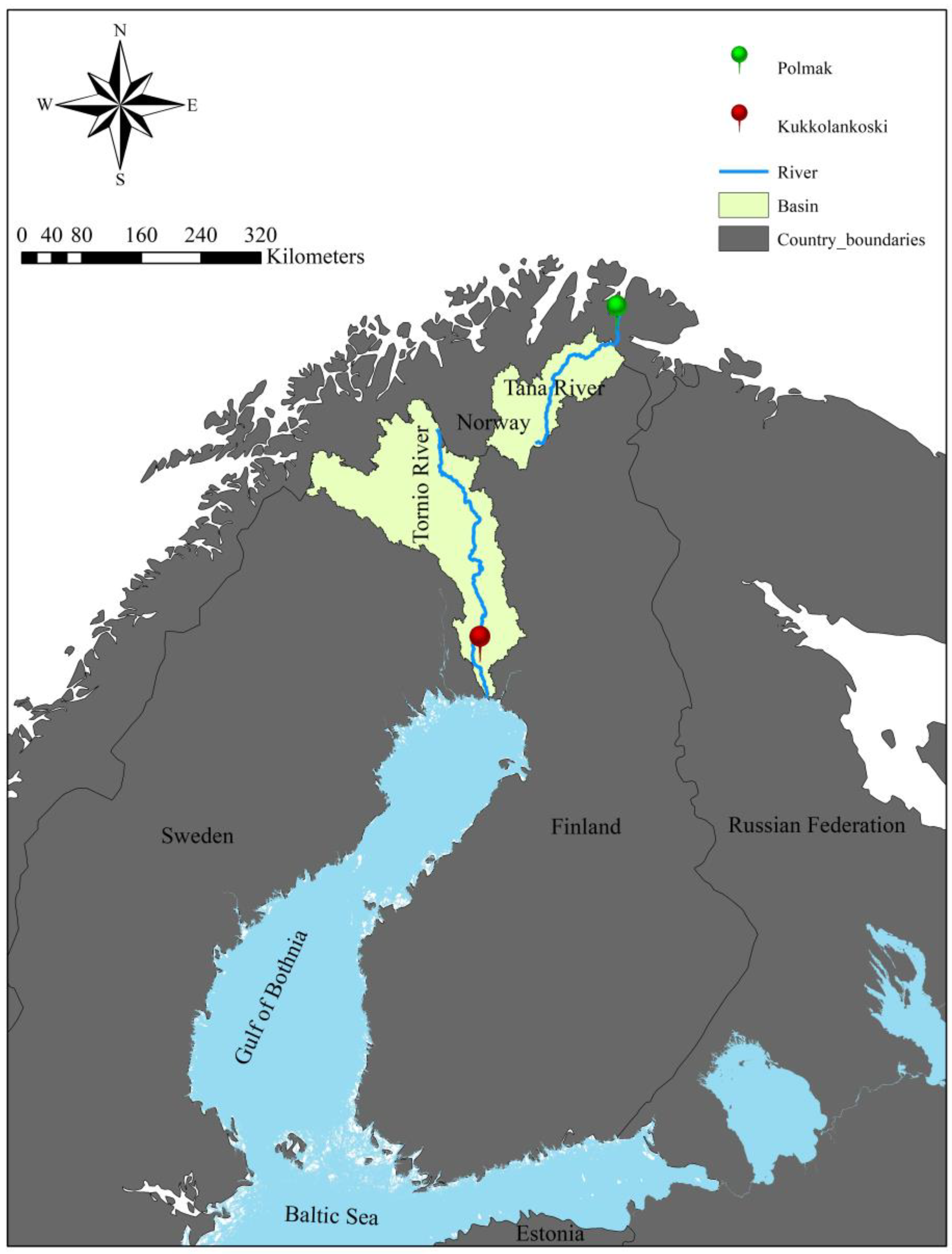
The northernmost region of Fennoscandia (i.e., Scandinavia and Finland) is where the Tana River Basin is situated (Figure 1). The catchment area is approximately 16,380 km2. The Tana River, serving as part of the official border between Norway and Finland for over 338 km, is one of the most important pristine rivers in Scandinavia and is the fifth largest in Norway, draining into the Barents Sea. The mouth and discharge of the Tana River are in Norway, although Finland occupies about one-third of its catchment area. The Tana River has an average annual discharge of 170 m3·s−1 [16]. It is a large upland drainage system that drains a sizable portion of the Finnmarksvidda in Norway and is a part of Fennoscandia’s subarctic region. Precambrian bedrock lies beneath the Tana Basin, primarily made up of granites, granulites, and various gneisses and schists. The northernmost region contains Eocambrian sedimentary rocks, including siltstones, shales, and sandstones [17]. The bedrock is mostly covered by glacial tills that were deposited during the most recent glaciation (i.e., Weichselian), with a few exceptions where deposits from the pre-Weichselian era predominate [18]. Several steep-sided fault valleys, including those of the tectonic Utsjoki and Tana, cut through this highland [17]. Even though elevations in Norway rarely rise above 500 m, some of the northern mountain peaks do, rising to just over 1000 m above sea level. In the climate classification system, this station belongs to the subpolar climate, with short, cool summers, severe winters, and no clear seasonality in precipitation. Polar tundra climates may be found at higher altitudes in the region. Annual precipitation is generally low for all weather stations, ranging from about 340–360 mm in Kautokeino (southwest of the Tana Basin) to 460 mm in Rustefjelbma in the Northeast. The Polmak gauging station on the Tana River, located at 70° N, 28° E, was chosen as the station to use for its extensive historical discharge data since 1911. There are a few years of data missing in this dataset, which are 1944, 1945, and 1946. This station falls under the subpolar climate classification system, which features short, cool summers, harsh winters, and no discernible seasonality in precipitation. All weather stations report low annual precipitation levels, with Kautokeino (in the Southwest of the Tana Basin) reporting about 340–360 mm, and Rustefjelbma (in the Northeast) reporting 460 mm. Snowmelt in the Tana Basin is often a swift process. The amount of snow lost daily in Kevo, Finland, may exceed 20 cm of snow depth. In just 10 days, up to 50% of the snowpack may melt away; in 30 days, 85% of the snowpack typically melts [19].
The Tornio River is the largest unregulated river in the Baltic Sea region. The river is 520 km long and its average annual discharge is 400 m3·s–1 [20]. It flows from north to south (Figure 1). The Tornio River is among the few rivers in the Baltic Sea area where Atlantic salmon still reproduce naturally. The Tornio River discharges in the northernmost part of the Gulf of Bothnia along the Finnish–Swedish border. The catchment area is 40,010 km2, which extends from the northern mountains of Sweden and Northwestern Finnish Lapland, southeast down through marshes and lowlands to the Gulf of Bothnia in the Baltic Sea. Around half of the catchment area is covered by forest, a fifth is mountains, and a tenth is marshland, with some agriculture in the lowlands. The river is ice covered, with the lowest river discharge from December to May. Usually, 1000–2000 m3·s−1 is released after the ice break-up in spring. The water temperature is typically above 10 °C at the lowest point in the river for three months per year (from early June to early September) [21].
There is little human disturbance, and the water quality is good. The mean annual precipitation in the catchment’s lowland regions is 550–600 mm; this increases to 800 mm closer to the Scandinavian highlands and to over 1000 mm in the Western highland regions [22]. Peak river discharge typically occurs in May and June, while the watershed is typically covered in snow from October to May [23]. The social disruption and damage brought on by spring floods started to draw more attention in the middle of the 1980s. Significant floods in 1615, 1677, 1968, and 1990 were recorded [22]. The most dangerous conditions arise when thick ice forms in the river mouth and acts as a dam, causing water levels to increase quickly behind it. Haparanda and Tornio now have a mechanism in place for forecasts and warnings. One of the 18 Swedish towns identified as having a “serious flood risk” is Haparanda [22]. In the Tornio River, the Kukkolankoski (on the Finnish side of the river, located at 65° N, 24° E) is considered as the case study. Although the dataset covers a century of data, there are some missing years from 1997–2002.
Every year, the Lions club members in Övertorneå and Haparanda, next to Tornio River, have a bet on when the ice breaks up. In Haparanda the BUD is observed when a frozen raft in the river moves. In Övertorneå location, a raft is an indicator as well, the time when the raft passes the bridge over the river indicates the break-up time. There are some issues regarding these indicators. For example, sometimes the ice melts, and water can move freely in some parts of the Tornio River before the raft starts to move. The raft in Övertorneå can also get stuck under the bridge, which occurred in 2010. There have also been sabotage attempts on the raft location [24]. Hence, this paper aims to find a unique solution for indicating the BUD from annual daily hydrographs.
2.2. Methodology
We have developed the RiTiCE tool in MATLAB that detects the BUD based on the annual daily hydrograph. Additionally, we have evaluated the discharge time series in terms of the duration and changes in the starting and ending periods of low and high flow. The case studies employed to develop RiTiCE are Tana and Tornio, two important pristine Nordic Rivers. Daily discharge data during 1911–2013 at Polmak station at the Tana River and during 1911–2017 at Kukkolankoski station at Tornio River were used. It is worth mentioning that the years are considered as 365 days. Therefore, “leap year correction” has been applied to the datasets so that leap years do not contain 29 February in their data. Besides, the data is sorted based on the conventional “water year” starting from 1 October to 30 September for each year.
2.2.1. Average-Annual-Daily-Discharge Year365
A long-term flow pattern on each station is needed to evaluate the flow alterations. We have introduced an average-annual-daily-discharge for all 100 years in each station called Year365. These data are obtained by averaging all the discharge data recorded in 100 years on every single date.
where Year365i stands for the average-annual-daily-discharge on a specific day, n is the total number of years, Qi is the discharge value of the specific day of each year, and i is the day from 1 to 365 for each year.
To our knowledge, comparing single water years with each other is impossible for a large dataset. To assess the large amount of data in a century, the data can be divided into time intervals of 5, 10, 20, 30, and 50 years, also enabling us to track the likely changes in the flow better periodically. Therefore, multiple periods in a century can be compared to each other. At each interval, the periods with the highest and lowest peak discharge are compared with the long-term flow pattern calculated as Year365. As Year365 represents the century, the extreme periods in each time interval can be detected during the comparison.
2.2.2. Seasonal Extremes
To introduce the flow timing characteristics, we consider periods of 90 days from each water year during which the flow is at its highest and lowest average value. The average value of discharge in 90 days (commonly known as a season) is a good representative of the flow condition, considering that there are two 90-day periods, one for the average highest flow and the other for the average lowest flow. The seasonal periods (i.e., 90-day periods) are calculated based on the “moving average”. Each day, the average is recalculated by including the new day’s data and dropping the oldest day’s data. On the other hand, Year365, explained above, has two extreme periods of averaged low and high flow of 90-day discharge. This is calculated based on the moving average, and the extreme seasons are extracted from the results as “low-flow” and “high-flow” periods. The discharge values corresponding to low flow can be used as a “threshold” to investigate the periods in each year during which the discharge values are lower than the low flow discharge. The trends of all analyses are calculated using a Mann–Kendall (M–K) test. Using the seasonal extremes in each year and comparing them to the Year365 seasonal extreme values, we come up with the results that can show how the onset and end date of the lowest and highest 90-day period occurs in each year compared with Year365. Moreover, we can track any probable shifts in these extremes in terms of timing.
2.2.3. Flow Extremes
We simply evaluate extreme discharge values (i.e., the absolute minimum and maximum discharge value of each water year) and their trends. The trends are considered from two aspects: (i) the absolute maximum and minimum discharge values; and (ii) their occurrence date. The confidence level of the trends is assessed using the Mann–Kendall trend test in MATLAB [25,26,27].
2.2.4. BUD Estimation
Finally, to detect the BUD on each annual daily hydrograph, the first order difference between each pair of consecutive discharge data is calculated:
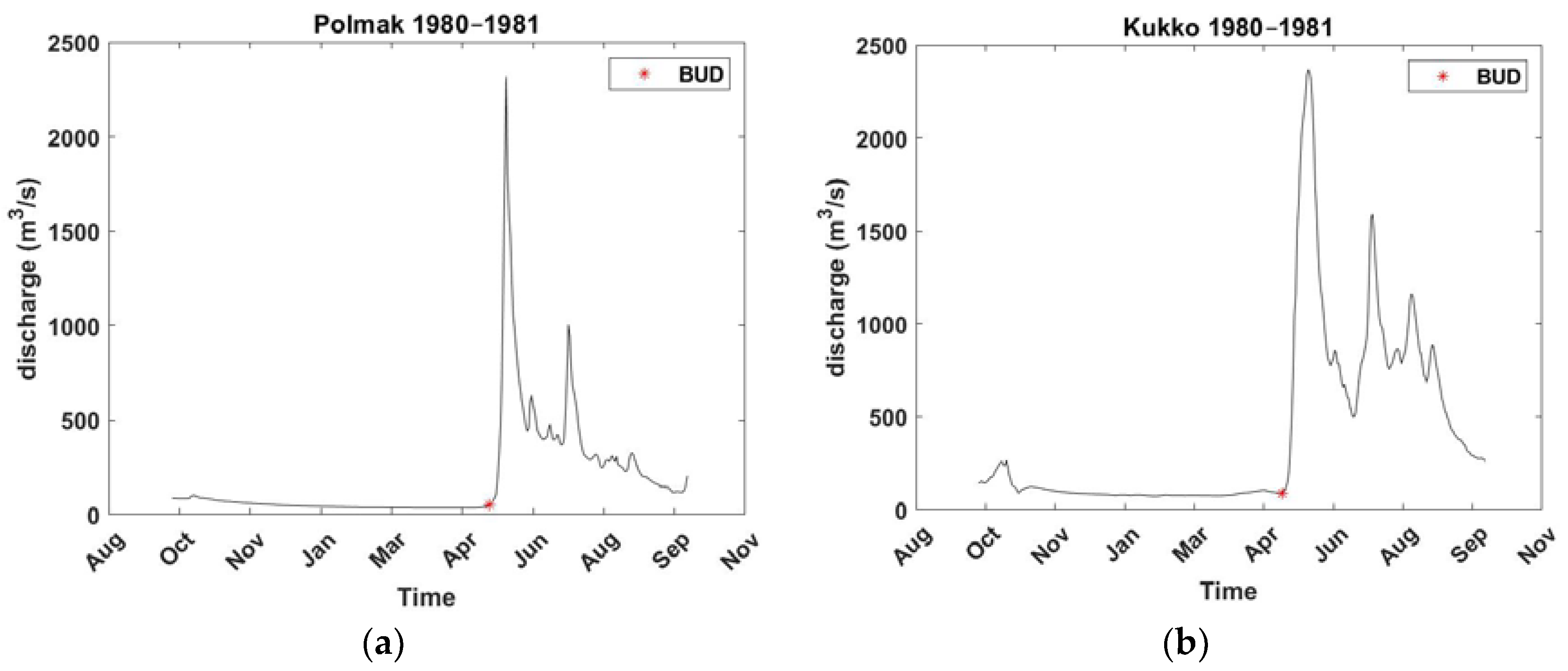
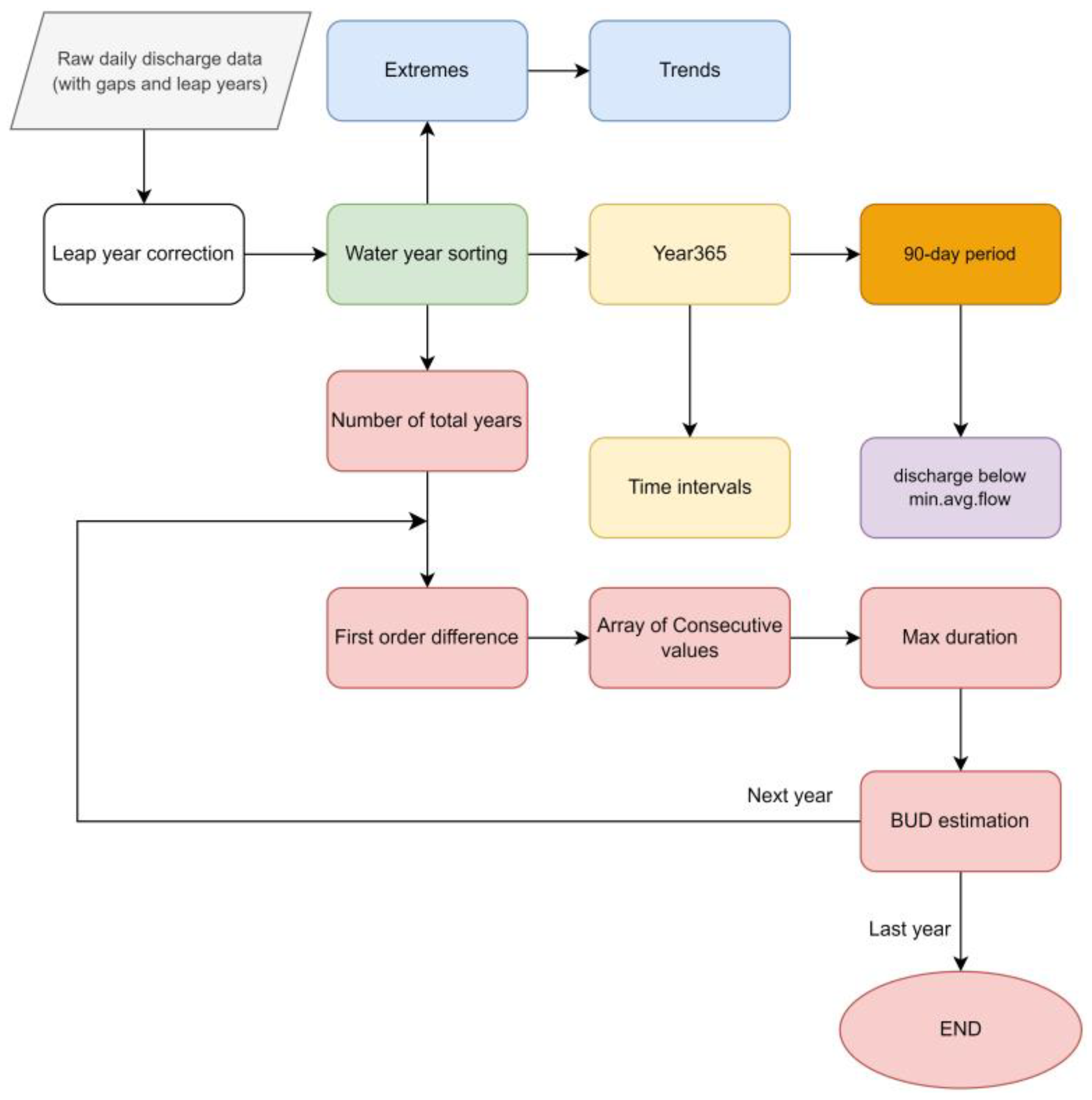
where, Δi is the “differenced” value, Q is the discharge value, and T is the time which equals 1 as we are using a daily hydrograph. Using the results from the series of differences, we observe that the point at which the discharge starts to rise in the spring has nearly equal values around 0. This occurs as the discharge time series follows a line with a gradient of around zero during winter. Therefore, the last value ending the consecutive zero gradient pair of points is considered the break-up point (Figure 2). The flowchart of the RiTiCE module is provided in Figure 3.
The break-up point is calculated for each year and station. However, only one observation dataset is available to verify the results. The Swedish Meteorological and Hydrological Institute (SMHI) has collected data on the break-up of ice on the Tornio River, specifically at the Karungiträsk station. These data are used to verify the results of the RiTiCE tool, which detects the BUD. The use of the data from the Karungiträsk station, which is located closest to the Kukkolankoski station, allows for the verification of the accuracy of the RiTiCE tool in determining the date of ice break-up on the Tornio River.
We propose to use the daily MODIS land surface temperature (LST) dataset presented in the study “Worldwide continuous gap-filled MODIS land surface temperature dataset” by Shiff et al. (2021) modified in Google Earth Engine (GEE) to detect the intersections of the positive temperature phase and river ice BUDs detected by the RiTiCE. The MODIS LST data provide high temporal and spatial resolution information on land surface temperatures, which is essential for understanding the relationship between temperature and river ice BUD. The MODIS daily LST dataset is available in GEE and can be easily imported into the platform. We have used the LST data from October 2002 onwards for each station.
3. Results
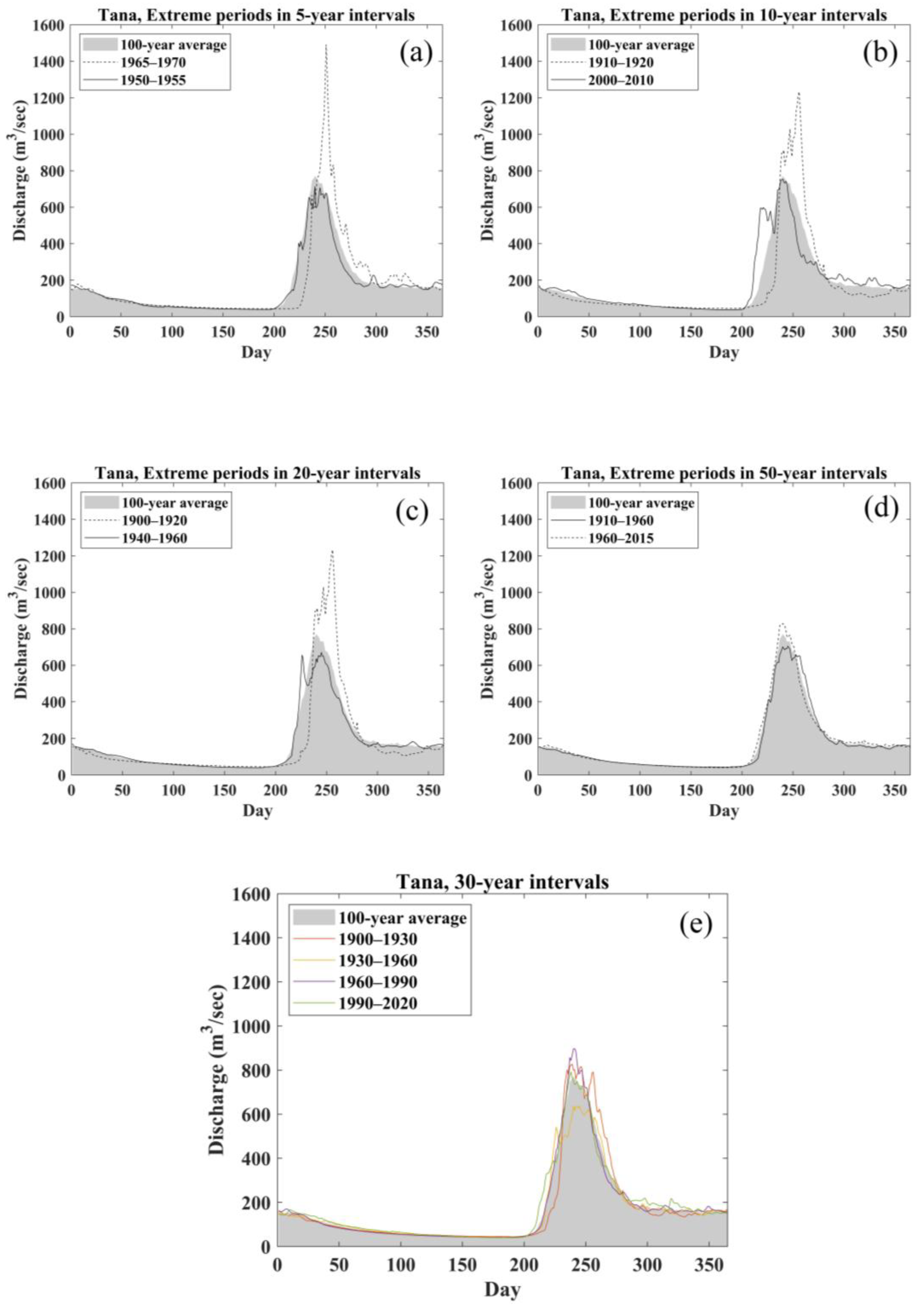
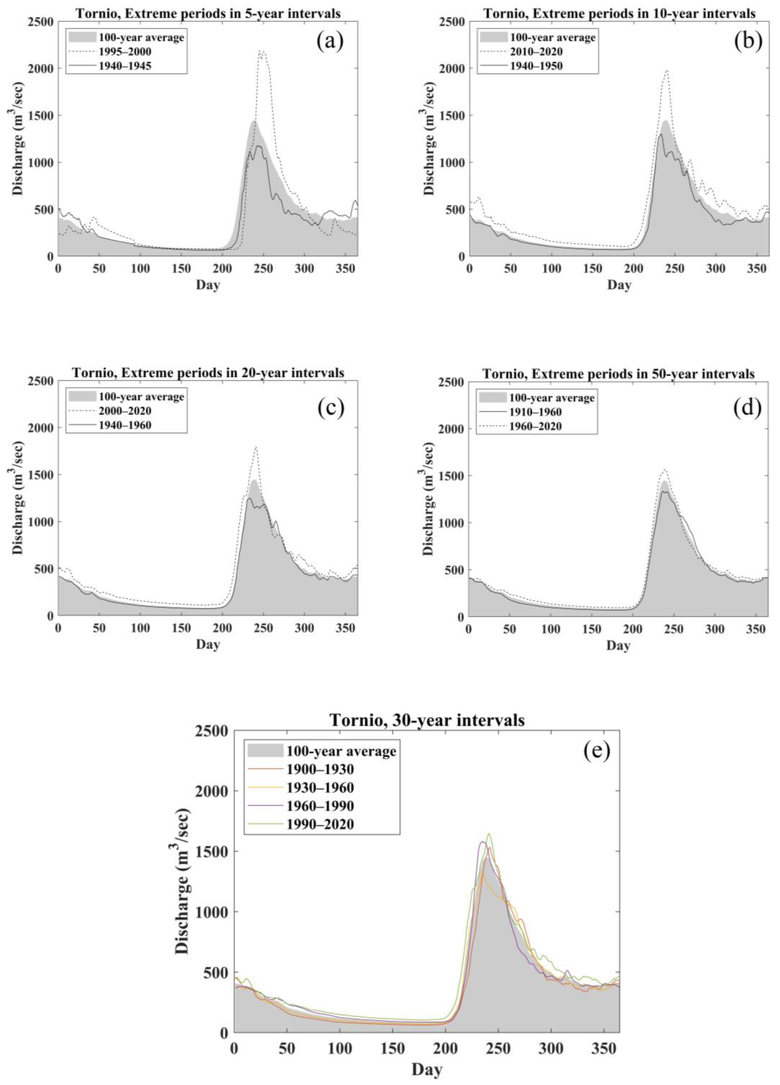
In 5-year intervals, two periods, 1965–1970 and 1950–1955, in the Tana River are extreme discharge periods with the highest and lowest discharge peaks, respectively. In the Tornio River, the highest discharge peak is during 1995–2000, and the lowest discharge peak is observed during 1940–1945 (Figure 4a and Figure 5a). In 10-year intervals, the highest and lowest discharge peaks occur in 1911–1920 and 2000–2010, respectively, in the Tana River (Figure 4b), and in the Tornio River, the highest and lowest discharge peaks occur in 2010–2017 and 1940–1950, respectively (Figure 5b). The result of the 20-year intervals shows that, in the Tana River, the highest discharge peak extreme period is 1911–1930, and the lowest discharge peak occurs in the 1940–1960 period (Figure 4c). In the Tornio River, the same extreme periods occur in the 2000–2017 and 1940–1960 periods, respectively (Figure 5c). For 50-year interval results of the Tana River, the highest discharge peak occurs in the first half (Figure 4d), although, in the Tornio River, the extreme period with the highest discharge peak occurs in the second half of the period (Figure 5d). Finally, the datasets are divided into 30-year intervals. The results show that the highest discharge peak is in 1960–1990 and the lowest discharge peak occurs in 1930–1960 in the Tana River. On the other hand, in the Tornio River, the highest and lowest discharge peaks occur in the 1990–2017 and 1930–1960 periods, respectively (Figure 4e and Figure 5e).
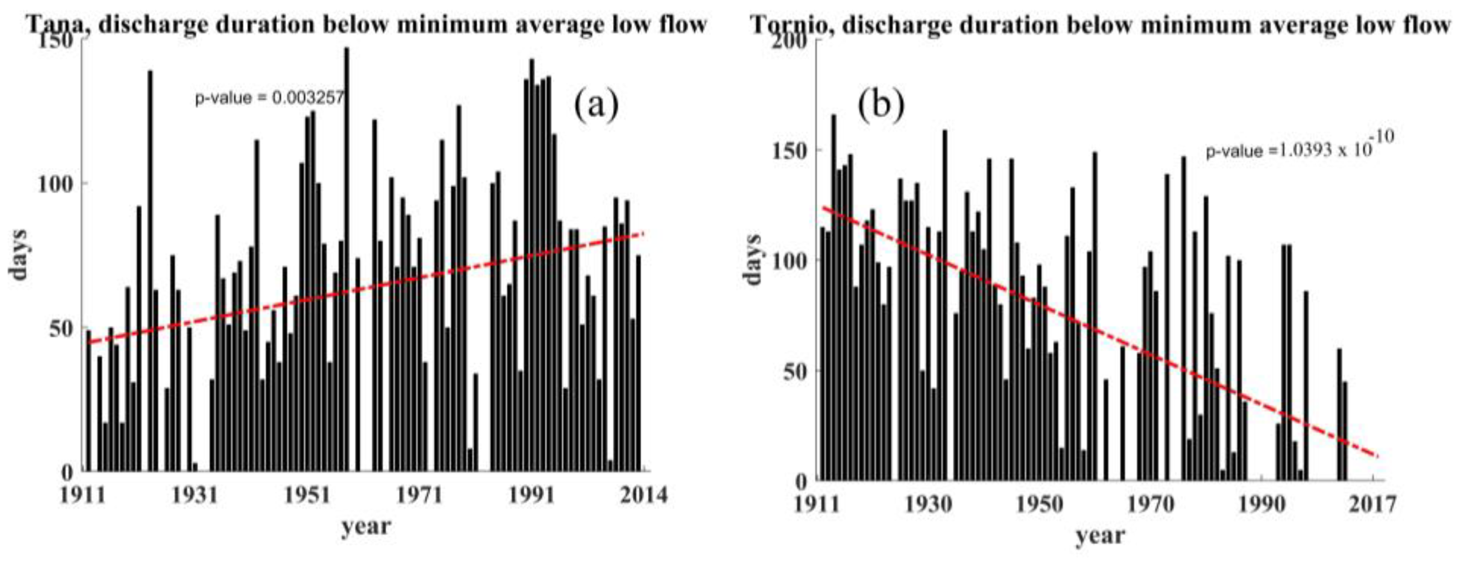
The duration of the period in which the discharge is lower than the minimum 90-day flow in Year365 has been significantly increased from 50–70 days to 100–140 days by a confidence level of 95% in the Tana River (Figure 6a). In contrast, in the Tornio River, the duration has been significantly decreased by a confidence level of 95%. In the first ten years, the duration is, on average, about 120 days, while the duration in the last ten years is about 50 days (Figure 6b).
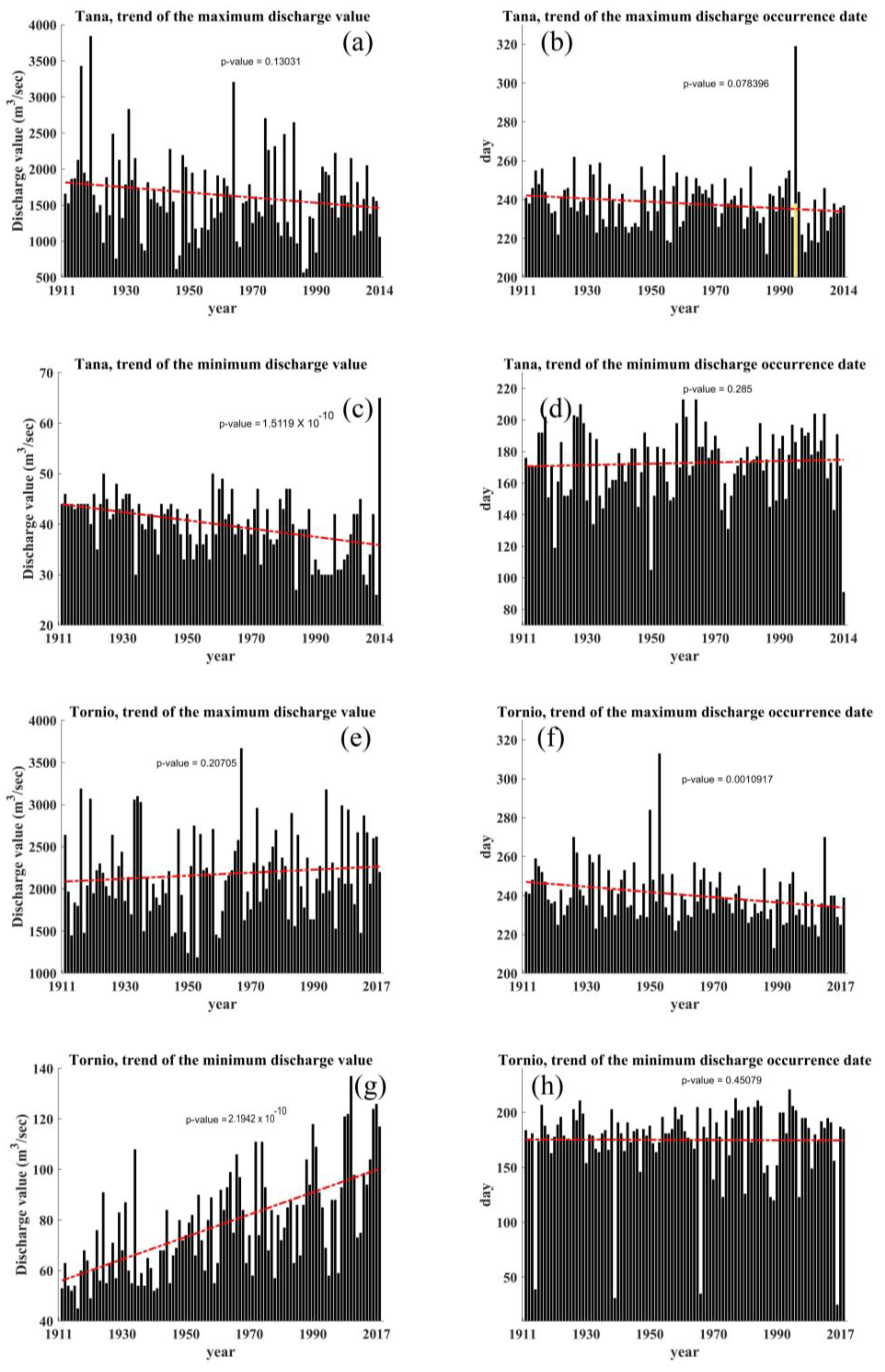
The M–K trend test does not show any significant trend in annual maximum discharge in the Tana River (Figure 7a). However, as the results show, the maximum discharge value tends to reduce in the latest years and the peaks are smaller than before. The Tornio River does not show any significant change in the annual maximum discharge either (Figure 7e). The Tana River also experiences a significant reduction in the annual minimum discharge with a confidence level of 95% (Figure 7c). However, the annual minimum discharge in the Tornio River significantly increases with the same confidence level (Figure 7g). It appears that the annual maximum discharge in the Tana River may have shifted backwards, but the trend is not significant (Figure 7b). The same shift takes place in Tornio with a confidence level of 95% (Figure 7f). The annual minimum discharge occurrence date in both rivers has not changed significantly.
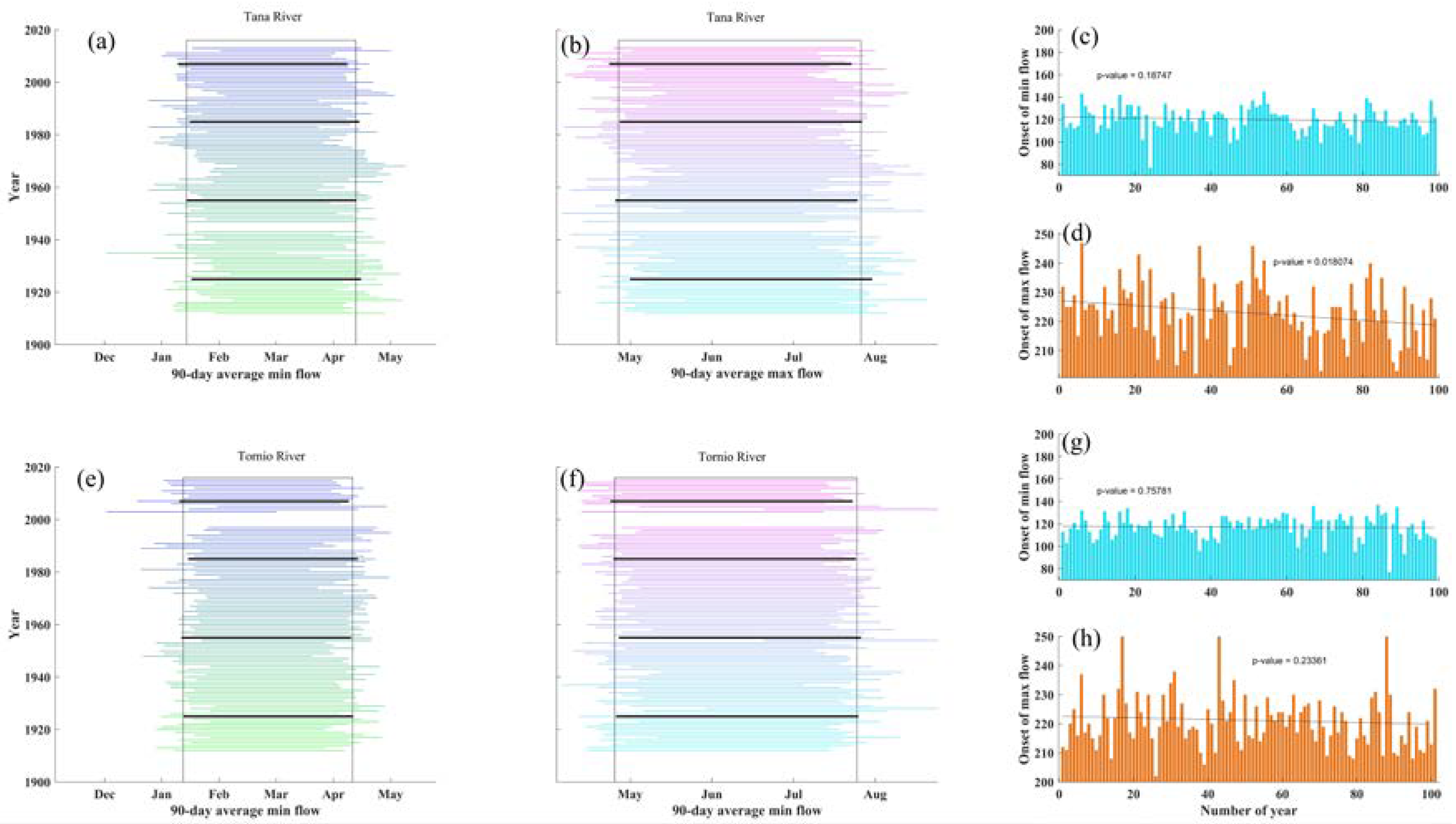
The seasonal extreme mean flow (whether maximum or minimum) in Year365 is shown by the black rectangle in Figure 8. In the Tana River, the lowest 90-day flow starts in the middle of January and ends in April, over an average of 100 years (Figure 8a). The highest 90-day flow starts in May and ends before August (Figure 8b). The same results occurs in the Tornio River for maximum and minimum 90-day flow over an average of 100 years (Figure 8e,f). Each dataset has been divided into 25-year periods and the results show that, in the Tana River, there has been a shift in the beginning and ending of the maximum and minimum 90-day flow every 25 years (Figure 8a,b,e,f). More precisely, recent years (1990–2017) have been experiencing more severe shifts in starting and ending dates. In other words, in both rivers, over later years, the minimum 90-day flow tends to occur sooner in January and the maximum 90-day period tends to occur before May. However, in the Tornio River, only the last 25 years reveal the shift; the Tana River shows that the first and second 25 years have shifted to the right (meaning that the minimum and maximum 90-day flows have occurred later than average).
The analyses illustrate that the starting date of the minimum flow in the Tana River varies from the 15th to 100th day from 1 October. However, the results do not show any significant change in the starting date of the minimum 90-day flow. On the other hand, there is a significant backward shift in the starting date of the maximum 90-day flow with a confidence level of 95% (Figure 8d). The analyses of the Tornio River do not show any significant shifts in either minimum or maximum 90-day flow (Figure 8g,h).
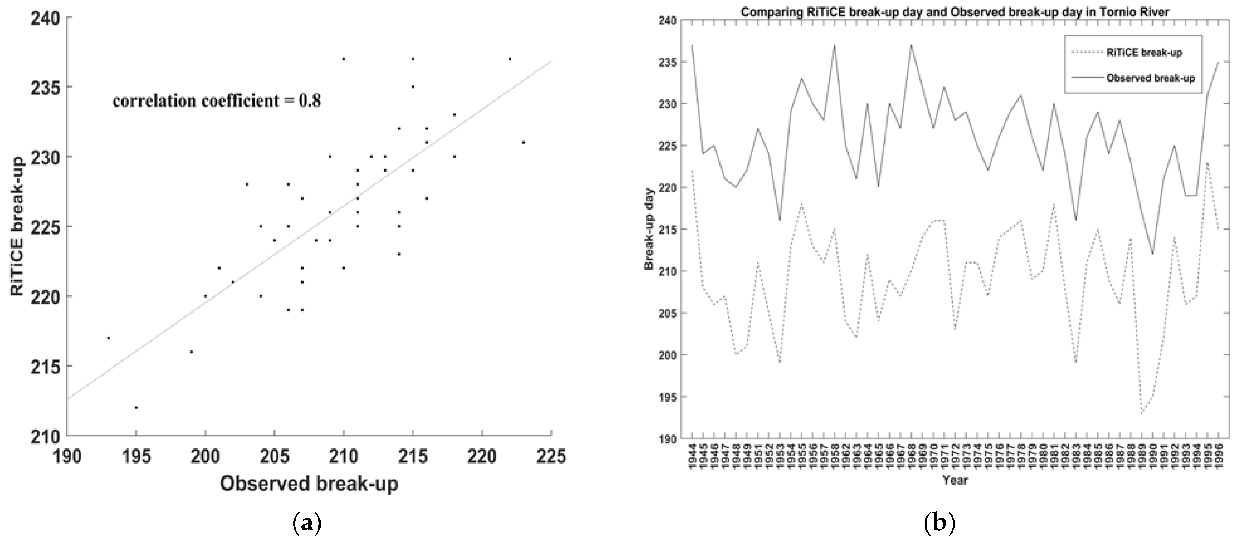
The BUD detection by the RiTiCE is verified by the real observation data on the Tornio River (Figure 9) for the available period (1944–1996). The results of the comparison between BUDs calculated by the RiTiCE and observed BUDs show a strong correlation of 0.8 (using the Pearson correlation coefficient).
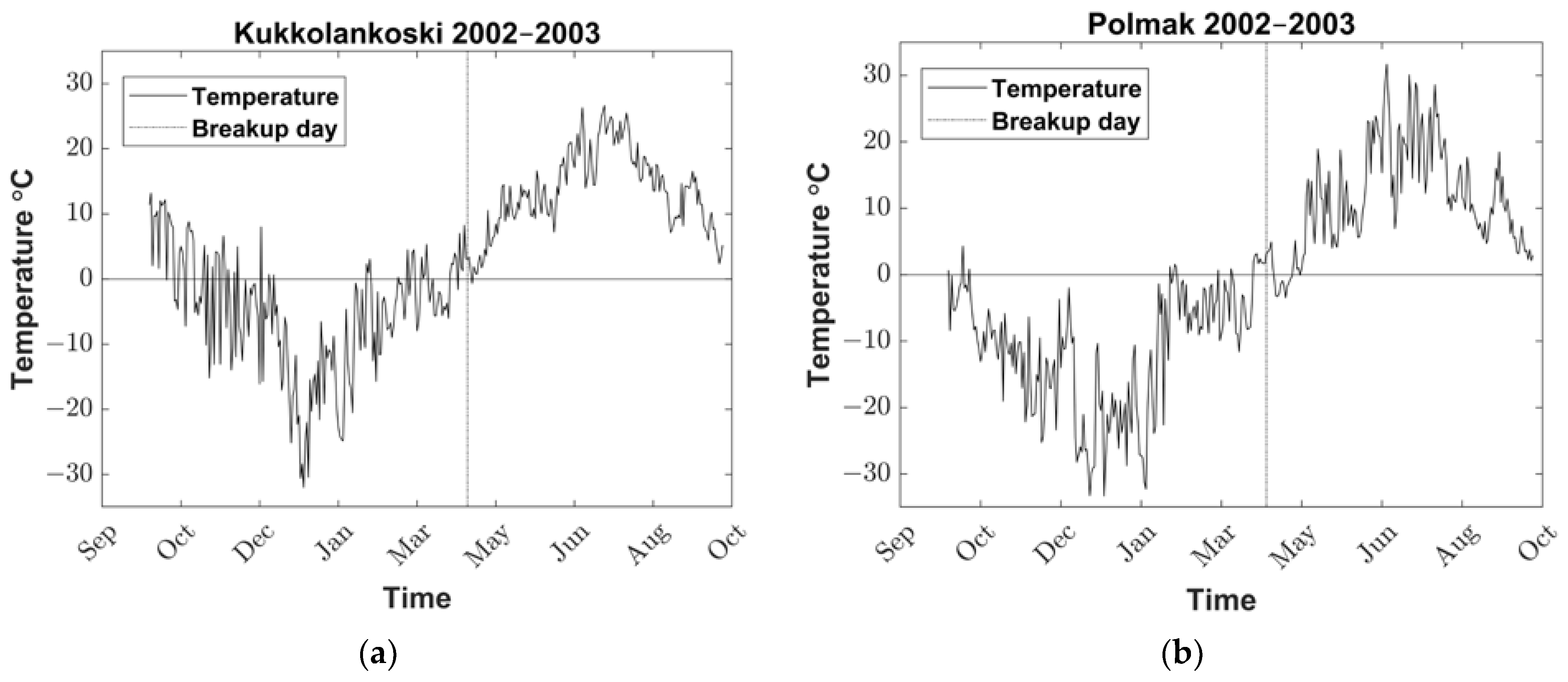
The results of our study show a clear relationship between annual daily temperature and the BUD calculated by the RiTiCE. Figure 10 illustrates that, as the positive phase of temperature begins, the break-up of the ice also starts to initiate. This supports our hypothesis that temperature plays a significant role in the timing of ice break-up. Detailed results for all years are included in the Supplementary Materials “Figures S3 and S4” folders.
4. Discussion
The study aims to find solutions for detecting the ice BUD from annual daily hydrographs and verifying the results by observed data. In addition, the study has developed indices to analyze the extreme values, trends, and probable shifts of flow characteristics through time.
It is worth mentioning that the long-term discharge datasets have some gaps. In the Tana River, data from the years 1944–1946, and in the Tornio River, data from the years 1997–2002, are missing. As the intervals are the average daily discharge values for a specific period, the periods that cover the missing data are not comparable to the remaining periods. For instance, in the Tana River, the interval of 20 years would result in two extreme periods for 1911–1930 and 1940–1960, from which the latter is considered the lowest discharge peak among other periods. This could be affected by missing data in that period. On the other hand, while comparing extreme periods in 5-year intervals in the Tornio River, the highest discharge peak belongs to the period 1995–2000, from which 3 years are missing. This leads to some uncertainties regarding the results, especially the intervals at which the extreme periods have been chosen.
The river ice break-up is induced by warm weather, including thermal degradation, initial fracturing, mobility, fragmentation, transport, jamming, and final clearance [28]. Although some or all these procedures may take place simultaneously to a certain extent, the break-up cycle can be seen as a sequence of distinct phases, such as pre-break-up, onset, driving, and washing [29]. Onset depends on many factors, including the morphology of the channel. Thus, it is common to see areas that have begun to change phases with areas that have not lost their ice. For different lakes and rivers, the BUD has long been done in Nordic Regions. However, not a certain indicator is found to address the break-up event equally. The main benefit of using the RiTiCE method is that it is based on our specific definition of the river break-up point, which is the point after which the discharge starts to increase in the spring. This method directly addresses our research question and provides a clear answer.
Another benefit of using the RiTiCE is that it is simple and easy to implement, based on a simple first-order difference of the consecutive values, and does not have any assumptions about the underlying distribution of the data. In addition, it also correlates well with the observed data. This suggests that the predictions made by the RiTiCE are closely aligned with the actual observed BUDs. However, it is also important to note that, although there is a significant correlation, on average, the BUDs calculated by the RiTiCE are 16 days before the observed data, owing to different definitions for ice break-up (i.e., raft movement by the Lion’s club vs. onset of discharge increase by the RiTiCE).
The methodology uses absolute maximum and minimum values for the discharge trends. It is assumed that the highest peak belongs to the spring discharge due to the snowmelt. However, in some years, a summer peak discharge is considered an outlier in the results as it is due to precipitation in the summer. In addition, periods below minimum flow correspond well with the results of discharge extremes. As it has been found that the minimum discharge values follow a significantly negative trend in the Tana River, the number of days during which the discharge value is below minimum flow (i.e., metrics from annual 90-day periods) increases significantly. The Tornio River has experienced a significant increment in its minimum discharge over the century, meaning the number of days during which the discharge value is below the minimum flow has decreased significantly.
The number of days in a year where the flow is below the minimum average low flow, of both the Tana and Tornio Rivers, has undergone significant changes, as shown in Figure 6. However, the trends are opposite in direction. The Tana River (as seen in Figure 6a) has experienced an increase in the number of days where the flow is below the minimum average low flow, indicating a higher likelihood of minimum flow in recent years. This is supported by the significant decreasing trend in the minimum discharge value of the Tana River, as seen in Figure 7c.
On the other hand, the Tornio River (Figure 6b) has experienced a decrease in the number of days where the flow is below the minimum average low flow, meaning that there is a lower chance of minimum flow in recent years. This is confirmed by the significant increasing trend in the minimum discharge value of the Tornio River, as seen in Figure 7g.
The current study can proceed by researching the reasons for such significant trends in these two stations. Obviously, several climatic factors can drive the river ice phenomena. As rivers react differently to climatic factors, not all models would work on every specific case.
5. Conclusions
River ice, and consequently, ice jam floods, are natural phenomena in cold climate regions. This study developed a tool called RiTiCE to examine the river flow timing characteristics and extreme discharges, along with detecting the break-up date (BUD). Two case studies are located on the Tornio and Tana Rivers on the Finnish borders of Sweden and Norway. The stations provide a century of daily discharge data, which are employed to evaluate the timing, and possible events shifts. Several characteristics have been developed for this purpose, considering Year365 as a metric to highlight the extreme events and corresponding years. From the same perspective on data, the 90-day periods show us that both low and high flows in the two rivers have a negative trend in their occurrence date, meaning the extreme seasonal discharges have tended to occur sooner in recent years. The Tana River does, however, show a negative trend in its annual minimum flow over the century, which contrasts with the Tornio River. The BUD detection by the RiTiCE has been verified through comparison with actual observation data in the Tornio River for 1944–1996. The comparison results demonstrate a strong correlation of 0.8 between the calculated and observed BUDs, indicating that the RiTiCE is an effective method for determining BUDs in this particular river. Finally, it was found that these two rivers have been experiencing a change in the duration of their low-flow periods. The Tana River shows a rise in the duration of its low-flow period, while the opposite is true for the Tornio River.
Supplementary Materials
The following supporting information can be downloaded at: https://www.mdpi.com/article/10.3390/w15050861/s1, Figure S1: Tornio River BUD results, Figure S2: Tana River BUD results, Figure S3: Tornio River temperature vs BUD results, Figure S4: Tana River temperature vs BUD results. RiTiCE-repository https://github.com/Aapoj/RiTiCE.git (accessed on 21 January 2023).
Author Contributions
Methodology, A.J.S. and A.T.H.; data analysis, A.J.S., A.A. and A.T.H.; validation, A.T.H., P.M.R. and B.K.; investigation, A.J.S., A.A., P.M.R., B.K. and A.T.H.; writing—original draft preparation, A.J.S. and A.A.; writing—review and editing, A.T.H., P.M.R. and B.K.; visualization, A.J.S.; supervision, A.T.H., P.M.R. and B.K. All authors have read and agreed to the published version of the manuscript.
Funding
This research was funded by the University of Oulu & the Academy of Finland Profi4 TTK Arcl (Grant No. 318930) and Maa- ja vesitekniikan tuki ry (MVTT, Grant No. 43588).
Data Availability Statement
All supporting data for this study are reported in the manuscript.
Conflicts of Interest
The authors declare no conflict of interest.
References
- Beltaos, S. River Ice Jams; Water Resources Publication: Littleton, CO, USA, 1995. [Google Scholar]
- Pawlowski, B. Internal structure and sources of selected ice jams on the lower Vistula River. Hydrol. Process. 2016, 30, 4543–4555. [Google Scholar] [CrossRef]
- Yang, X.; Pavelsky, T.M.; Allen, G.H. The past and future of global river ice. Nature 2020, 577, 69–73. [Google Scholar] [CrossRef] [PubMed]
- Beltaos, S.; Prowse, T.D. Climate impacts on extreme ice-jam events in Canadian rivers. Hydrol. Sci. J. 2001, 46, 157–181. [Google Scholar] [CrossRef]
- Chokmani, K.; Khalil, B.; Ouarda, T.; Bourdages, R. Estimation of river ice thickness using artificial neural networks. In Proceedings of the 14th Workshop Hydraulics Ice Covered Rivers, CGU HS/CRIPE, Quebec City, QC, Canada, 19–22 June 2007; p. 12. [Google Scholar]
- Carr, M.L.; Vuyovich, C.M. Investigating the effects of long-term hydro-climatic trends on Midwest ice jam events. Cold Reg. Sci. Technol. 2014, 106, 66–81. [Google Scholar] [CrossRef]
- Prowse, T.D.; Bonsal, B.R.; Duguay, C.R.; Lacroix, M.P. River-ice break-up/freeze-up: A review of climatic drivers, historical trends and future predictions. Ann. Glaciol. 2007, 46, 443–451. [Google Scholar] [CrossRef] [Green Version]
- Beltaos, S. Onset of river ice breakup. Cold Reg. Sci. Technol. 1997, 25, 183–196. [Google Scholar] [CrossRef]
- Kusatov, K.I.; Ammosov, A.P.; Kornilova, Z.G.; Shpakova, R.N. Anthropogenic factor of ice jamming and spring breakup flooding on the Lena River. Russ. Meteorol. Hydrol. 2012, 37, 392–396. [Google Scholar] [CrossRef]
- Chen, Y.; She, Y. Long-term variations of river ice breakup timing across Canada and its response to climate change. Cold Reg. Sci. Technol. 2020, 176, 103091. [Google Scholar] [CrossRef]
- Lesack, L.F.; Marsh, P.; Hicks, F.E.; Forbes, D.L. Local spring warming drives earlier river-ice breakup in a large Arctic delta. Geophys. Res. Lett. 2014, 41, 1560–1567. [Google Scholar] [CrossRef]
- Gohari, A.; Shahrood, A.J.; Ghadimi, S.; Alborz, M.; Patro, E.R.; Klöve, B.; Haghighi, A.T. A century of variations in extreme flow across Finnish rivers. Environ. Res. Lett. 2022, 17, 124027. [Google Scholar] [CrossRef]
- Haghighi, A.T.; Kløve, B. Development of a general river regime index (RRI) for intra-annual flow variation based on the unit river concept and flow variation end-points. J. Hydrol. 2013, 503, 169–177. [Google Scholar] [CrossRef]
- Poff, N.L.; Olden, J.D.; Merritt, D.M.; Pepin, D.M. Homogenization of regional river dynamics by dams and global biodiversity implications. Proc. Natl. Acad. Sci. USA 2007, 104, 5732–5737. [Google Scholar] [CrossRef] [PubMed] [Green Version]
- Rokaya, P.; Budhathoki, S.; Lindenschmidt, K.-E. Trends in the timing and magnitude of ice-jam floods in Canada. Sci. Rep. 2018, 8, 5834. [Google Scholar] [CrossRef] [PubMed] [Green Version]
- Annamo, E.; Kristiansen, G. Challenges in flood risk management planning. In An Example of a Flood Risk Management Plan for the Finnish-Norwegian River Tana; Norwegian Water Resources and Energy Directorate: Oslo, Norway, 2012. [Google Scholar]
- Mansikkaniemi, H. Deposits of Sorted Material in the Inarijoki-Tana River Valley in Lapland; Turku University (Finland) Institutum Geographicum: Turku, Finland, 1970. [Google Scholar]
- Olsen, L.; Reite, A.; Riiber, K.; Sørensen, E. Finnmark County, Map of Quaternary Geology, Scale 1: 500,000 with Description; Geological Survey of Norway: Trondheim, Norway, 1996. [Google Scholar]
- Dankers, R. Sub-Arctic Hydrology and Climate Change: A Case Study of the Tana River Basin in Northern Fennoscandia. Ph.D. Thesis, Utrecht University Repository, Utrecht, Netherlands, 2002. [Google Scholar]
- Romakkaniemi, A. Conservation of Atlantic Salmon by Supplementary Stocking of Juvenile Fish; Helsingin yliopisto: Helsinki, Finland, 2008. [Google Scholar]
- Hyvärinen, P.; Rodewald, P. Enriched rearing improves survival of hatchery-reared Atlantic salmon smolts during migration in the River Tornionjoki. Can. J. Fish. Aquat. Sci. 2013, 70, 1386–1395. [Google Scholar] [CrossRef]
- Rayner, D.; Achberger, C.; Chen, D. A multi-state weather generator for daily precipitation for the Torne River basin, northern Sweden/western Finland. Adv. Clim. Chang. Res. 2016, 7, 70–81. [Google Scholar] [CrossRef]
- Carlsson, B. Some Facts about the Torne and Kalix River Basins; Hydrology Report; Swedish Meteorology and Hydrology Institute: Norrköping, Sweden, 1999. [Google Scholar]
- Persson, G. Islossning i Torneälven; SMHI: Norrköping, Sweden, 2012. [Google Scholar]
- Kendall, M.G. Further contributions to the theory of paired comparisons. Biometrics 1955, 11, 43–62. [Google Scholar] [CrossRef]
- Mann, H.B. Nonparametric tests against trend. Econom. J. Econom. Soc. 1945, 13, 245–259. [Google Scholar] [CrossRef]
- Fatichi, S. Mann-kendall test. Retrieved 2009, 3, 2021. [Google Scholar]
- Scrimgeour, G.J.; Prowse, T.D.; Culp, J.M.; Chambers, P.A. Ecological effects of river ice break-up: A review and perspective. Freshw. Biol. 1994, 32, 261–275. [Google Scholar] [CrossRef]
- Beltaos, S. Threshold between mechanical and thermal breakup of river ice cover. Cold Reg. Sci. Technol. 2003, 37, 1–13. [Google Scholar] [CrossRef]
Figure 1.
The study area, the Tana and Tornio Rivers located at the Finnish border with Norway and Sweden. The river gauges used in the study are Polmak (green) and Kukkolankoski (red).
Figure 1.
The study area, the Tana and Tornio Rivers located at the Finnish border with Norway and Sweden. The river gauges used in the study are Polmak (green) and Kukkolankoski (red).

Figure 2.
(a) Break-up detection in Polmak, Tana River; (b) break-up detection in Kukkolankoski, Tornio River. The break-up detection results are available in Supplementary Materials Figure S1 and S2 folders.
Figure 2.
(a) Break-up detection in Polmak, Tana River; (b) break-up detection in Kukkolankoski, Tornio River. The break-up detection results are available in Supplementary Materials Figure S1 and S2 folders.

Figure 3.
Flowchart of the RiTiCE; the modules come in different colors.

Figure 4.
Extreme average annual discharge time series for different 30-year periods (a–e) for the Tana River.
Figure 4.
Extreme average annual discharge time series for different 30-year periods (a–e) for the Tana River.

Figure 5.
Extreme average annual discharge time series in different period intervals (a–e) for the Tornio River.
Figure 5.
Extreme average annual discharge time series in different period intervals (a–e) for the Tornio River.

Figure 6.
The trend of discharge duration below the minimum average low flow from Year365 for each river.
Figure 6.
The trend of discharge duration below the minimum average low flow from Year365 for each river.

Figure 7.
The trend of annual discharge extremes and their corresponding date for Tana and Tornio.

Figure 8.
90-day periods of low and high flow, (a) low flow in the Tana River, (b) high flow in the Tana River, (c) trend of low flow starting date in the Tana River, (d) trend of high flow starting date in the Tana River, (e) low flow in the Tornio River, (f) high flow starting date in the Tornio River, (g) trend of low flow starting date in the Tornio River, (h) trend of high flow starting date in the Tornio River.

Figure 9.
(a) Strong positive correlation between calculated BUDs by the RiTiCE and observed BUDs in Tornio River; (b) Comparison of calculated vs observed BUDs.
Figure 9.
(a) Strong positive correlation between calculated BUDs by the RiTiCE and observed BUDs in Tornio River; (b) Comparison of calculated vs observed BUDs.

Figure 10.
(a) Intersection of BUD in Kukkolankoski station, and the start of the temperature-positive phase during October 2002–September 2003; (b) Intersection of BUD in Polmak station, and the start of the temperature-positive phase during October 2002–September 2003.
Figure 10.
(a) Intersection of BUD in Kukkolankoski station, and the start of the temperature-positive phase during October 2002–September 2003; (b) Intersection of BUD in Polmak station, and the start of the temperature-positive phase during October 2002–September 2003.

Disclaimer/Publisher’s Note: The statements, opinions and data contained in all publications are solely those of the individual author(s) and contributor(s) and not of MDPI and/or the editor(s). MDPI and/or the editor(s) disclaim responsibility for any injury to people or property resulting from any ideas, methods, instructions or products referred to in the content. |
© 2023 by the authors. Licensee MDPI, Basel, Switzerland. This article is an open access article distributed under the terms and conditions of the Creative Commons Attribution (CC BY) license (https://creativecommons.org/licenses/by/4.0/).
Share and Cite
MDPI and ACS Style
Jalali Shahrood, A.; Ahrari, A.; Rossi, P.M.; Klöve, B.; Torabi Haghighi, A. RiTiCE: River Flow Timing Characteristics and Extremes in the Arctic Region. Water 2023, 15, 861. https://doi.org/10.3390/w15050861
AMA Style
Jalali Shahrood A, Ahrari A, Rossi PM, Klöve B, Torabi Haghighi A. RiTiCE: River Flow Timing Characteristics and Extremes in the Arctic Region. Water. 2023; 15(5):861. https://doi.org/10.3390/w15050861
Chicago/Turabian StyleJalali Shahrood, Abolfazl, Amirhossein Ahrari, Pekka M. Rossi, Björn Klöve, and Ali Torabi Haghighi. 2023. "RiTiCE: River Flow Timing Characteristics and Extremes in the Arctic Region" Water 15, no. 5: 861. https://doi.org/10.3390/w15050861
Note that from the first issue of 2016, this journal uses article numbers instead of page numbers. See further details here.