Article

Simulation of Crop Productivity for Guinea Grass (Megathyrsus maximus) Using AquaCrop under Different Water Regimes

by
César Augusto Terán-Chaves
1,*,
José Edwin Mojica-Rodríguez
2,
Alexander Vega-Amante
2 and
Sonia Mercedes Polo-Murcia
2
1
Corporación Colombiana de Investigación Agropecuaria—AGROSAVIA, Centro de Investigación Tibaitatá—km 14, Vía Mosquera-Bogotá, Mosquera 250047, Colombia
2
Corporación Colombiana de Investigación Agropecuaria—AGROSAVIA, Centro de Investigación Motilonia—km 5 Vía a Becerril, Agustín Codazzi 202050, Colombia
*
Author to whom correspondence should be addressed.
Water 2023, 15(5), 863; https://doi.org/10.3390/w15050863
Submission received: 27 January 2023 / Revised: 16 February 2023 / Accepted: 17 February 2023 / Published: 23 February 2023
(This article belongs to the Special Issue Model-Based Irrigation Management)

Abstract

:
The perennial herbaceous forage crops’ (PHFC) biomass as bioindustry feedstock or source of nutrients for ruminants is very important from their final utilization point of view. In 2022, the AquaCrop-FAO version 7.0 model has been opened for PHFC. In this context, this study aimed to test for the first time the ability of the AquaCrop-FAO model to simulate canopy cover (CC), total available soil water (TAW), and biomass (B) of Guinea grass (Megathyrsus maximus cv. Agrosavia sabanera) under different water regimes at the Colombian dry Caribbean, South America. The water regimes included L1—irrigation based on 80% field capacity (FC), L2—irrigation based on 60% FC, L3—irrigation based on 50% FC, L4—irrigation based on 40% FC, L5—irrigation based on 20% FC, and L6—rainfed. The AquaCrop model uses the normalized water productivity—WP* (g m−2)—to estimate the attainable rate of crop growth under water limitation. The WP* for Guinea grass was 35.9 ± 0.42 g m−2 with a high coefficient of determination (R2 = 0.94). The model calibration results indicated the simulated CC was good (R2 = 0.84, RMSE = 17.4%, NRMSE = 23.2%, EF = 0.63 and d = 0.91). In addition, cumulative biomass simulations were very good (R2 = 1.0, RMSE = 5.13 t ha−1, NRMSE = 8.0%, EF = 0.93 and d = 0.98), and TAW was good (R2 = 0.85, RMSE = 5.4 mm, NRMSE = 7.0%, EF = 0.56 and d= 0.91). During validation, the CC simulations were moderately good for all water regimes (0.78 < R2 < 0.97; 12.0% < RMSE < 17.5%; 15.9% < NRMSE < 28.0%; 0.47 < EF < 0.87; 0.82 < d < 0.97), the cumulative biomass was very good (0.99 < R2 < 1.0; 0.77 t ha−1 < RMSE < 3.15 t ha−1; 2.5% < NRMSE < 21.9%; 0.92 < EF < 0.99; 0.97 < d < 1.0), and TAW was acceptable (0.70 < R2 < 0.90; 5.8 mm < RMSE < 21.7 mm, 7.6% < NRMSE < 36.7%; 0.15 < EF < 0.58 and 0.79 < d < 0.9). The results of this study provide an important basis for future research, such as estimating biomass production of high-producing grasses in tropical environments, yield effects under scenarios of climate variability, and change based on the presented parameterization and considering a wide range of environments and grazing variations.

1. Introduction

Production systems that combine dairy and beef cattle (i.e., “mixed cattle systems”), or double purpose, perform economic and sociocultural functions that contribute to the welfare of communities in the rural zones of Latin America [1]. Colombian bovine production is an important economic sector; this sector contributed to 6% of employment and 1.6% of the national GDP (gross domestic product) in 2021 [2]. Tropical pastures are the main basis for feeding ruminants in different zones of Colombia. Introduced and native grasses extend for ∼34.4 Mha of the national territory’s [3] surface, and they are found across a variety of ecosystems.
The Colombian dry Caribbean is an ecosystem that has been used regularly for dual-purpose cattle systems, developed mainly for extensive grazing [4]. Guinea grass (Megathyrsus maximus) is a grass C4 of worldwide importance, tolerant to different types of stress and highly competitive with the native species in tropical environments [5]; in the Colombian dry Caribbean, Guinea grass (Megathyrsus maximus) cultivars Mombasa, Tanzania, and Agrosavia sabanera (AS) have been widely established for ruminant feeding [6]. The cultivar AS was introduced for the first time in the Colombian dry Caribbean in 2016 and was quickly extended; the main characteristics of AS are the good production of forage (>2000 kg MS ha−1 cut−1), high crude protein content (13.3%), good tolerance to shadow and moderate tolerance to pest insects such as Blissus sp. and Aenolamia reducta [7].
The growth and quality of pastures are directly associated with physiological dynamics that require water contribution to keep the turgidity pressure, the efficiency of the photosystems, and nutritional quality [8]. Seasonality and climate variability are two of the factors that can negatively influence the production of tropical grasses. The forage availability of Megathyrsus maximus cv. Agrosavia sabanera decreases significantly by the effects of the prolonged dry season, which is evidenced by going from 4128.8 kg MS ha−1 cut−1 in the rainy season to 1200.7 kg MS ha−1 cut−1 in the dry season, with 42 days of regrowth [9].
The lack of strategies for mitigation and adaptation of agriculture in a changing environment can reduce the economic value of grasslands and can even be a threat to food security [10,11]. Therefore, quantifying temporal and spatial patterns of the performance of dry matter of Guinea grass in the face of the growing frequency of extreme weather and climate events is a key aspect to improving the process of decision-making by Colombian farmers. The crop models are useful tools to understand the agricultural systems and the interactions between their edaphic, climatic and agronomic components.
Using models of simulation of tropical pastures can provide elements to pasture management, forage production, and the efficiency of grazing in climate variability scenarios [12,13], which has an important economic effect, by considerably reducing the necessity of expensive experiments in the long-term [13]. Studies to adapt mechanistic models for tropical pasture and forage are limited, but their applications are promising, both in the investigation and the management of cattle systems; the selection of the model depends on the purposes of simulation and the information (data) available [14].
In the last few years, with performances barely satisfactory, they have been calibrated and validated for growing simulations of different genres of grasses (Panicum, Brachiaria, Cynodon, Paspalum, Megathryrsus, Urochloa) and tropical conditions using the models ALMANAC [15], CROPGRO-PFM Perennial Forage of DSSAT (Decision Support System for Agrotechnology Transfer) [16,17,18], APSIM (Agricultural Production Systems sIMulator) [19,20], Orchidee-GM (Orchidee Grassland Management) [20], APSIM-Tropical Pasture for Megathyrsus maximus cv. Mombaça [21]. In Colombia, the model AquaCrop-FAO was parameterized for pasture ryegrass (Lolium perenne) [22] and fodder oats (Avena sativa) in high tropical conditions [23].
The AquaCrop model is a water-driven model developed by the Food and Agriculture Organization of the United Nations (FAO) that simulates the evolution of crop biomass and crop yield in the function of soil water content in the root zones [24]. To facilitate its use, AquaCrop needs a quantity relatively reduced of parameters and, in its majority, intuitive input variables [25]. Version 7.0 (2022) of AquaCrop contains new modules to simulate the growth and production of perennial herbaceous forage crops [26].
The Colombian dry Caribbean is a semi-arid region, the water deficit is considerably high, and the annual precipitation average is 1508.5 mm, while the reference evapotranspiration reaches an average of 1879.8 mm per year−1 [27]. The forage biomass, as well as its nutritional values, depends on a large measure of the annual precipitation [28]; therefore, simulating the growth of tropical pastures in this region is relevant to predicting the supply of bovine feed and the yield gaps.
The main aim of this research was to calibrate and validate AquaCrop model version 7.0 to simulate Guinea grass growth and production (Megathyrsus maximus cv. Agrosavia sabanera) under different irrigation levels cultivated in tropical semi-arid conditions. The performance of the AquaCrop model has been evaluated based on field data collected during two growing seasons (2020/21 and 2021/22). To date, relatively few studies have evaluated tropical pasture simulation models under different irrigation regimes. The results reported in this study provide an initial foundation for further research aimed at adapting the AquaCrop model for tropical pastures and for other perennial herbaceous forage crops (PHFC). The parameterization of the AquaCrop model for Guinea grass in our local conditions can be used to extrapolate a more extensive range of management practices and climatic conditions, as well as to derive strategies for efficient use of the water and the soil. Furthermore, it can bring added value for enriching the model AquaCrop database.

2. Materials and Methods

2.1. Site Description

The data set used in this study was obtained in a field experiment conducted over two growing seasons (from 2020 to 2022) at Motilonia Research Center of AGROSAVIA, located in the Department of Cesar, Colombia (10°2′ N, 73°16′ W, 339 m.a.s.l elevation). The climate is semi-arid, with high temperatures, high aridity index (>0.75), and limited soil humidity. Long-term climatic data (1980–2019) shows an annual average of 1508.5 mm of precipitation received mainly during the months from September–November and 1879.6 mm per year reference evapotranspiration, with maximum average temperatures between 32 °C and 38 °C and a minimum temperature of 24 °C (Figure 1).

2.2. Experimental Details and Crop Management

The data set used in this study was obtained from a field experiment performed during two growing seasons. The first season (2020/21) went from 19 June 2020 to 24 February 2021, and the second season (2021/22) was from 17 December 2021 to 4 June 2022. The duration of the season 2021/22 experiment was less than 2020/21 due to climatic conditions; the situation affected crop development and prevented us from capturing information.
In both seasons, the experiments were laid out in a randomized complete block design with six water regimes and eight replications, in 30 m2 plots. Irrigation was carried out using a linear source sprinkler irrigation system [29]. The irrigation regimes included L1—irrigation based on 80% field capacity (FC), L2—irrigation based on 60% FC, L3—irrigation based on 50% FC, L4—irrigation based on 40% FC, L5—irrigation based on 20% FC, and L6—rainfed. To allow correct germination and crop establishment, all the treatments were completely irrigated to cover the crops’ needs until emergency at 90% of the seed sown. Guinea grass (Megathyrsus maximus cv. Agrosavia sabanera) was planted as 48 plots (10 m × 3 m each), aligned perpendicular to the center line of the irrigation heads; the spacing was 50 cm between furrows and 100 seeds m−1, approximately. The plant population was 2,594,972 plants ha−1 for the first season to 2,001,101 plants ha−1 in the second season.
The pests and diseases were controlled carefully, and weeds were not allowed to develop in the field. As a crop weed management strategy, sowing of Guinea grass was made the day after finishing the soil preparation. We used pre-emergence herbicide 2,4-Dichlorophenoxyacetic (2,4-D) for broadleaf weed control, which was applied at a dose of 1 liter per hectare. Moreover, we applied halosulfuron-methyl, a post-emergence herbicide (20 days after emergence), at 150 g per hectare for reducing the number and mass of tubers of Cyperus rotundus L.
The management field practices were to ensure optimum soil fertility. Nitrogen (N), phosphorus (P2O5), potassium (K2O), and magnesium (MgSO4.7H2O) fertilizers were applied three times. The first moment was 15 days after emergence (DAE), the second moment was at 30 DAE, and the third moment was at 45 DAE. The detailed different fertilizer doses that were applicated with the same amount in the two growing seasons of Guinea Grass are shown in Table 1.
The pasture was subjected to frequent defoliations to 15 cm above the soil surface, with total removal of harvested material approximately every 42 days, according to the best interval defoliations for the region. The frequent defoliations and the irrigation levels created a wide array of canopy cover.

2.3. Description of AquaCrop Model

The Food and Agriculture Organization of the United Nations—FAO—developed the model of water productivity for AquaCrop [30]. The model consists of climate, crops, and soil management modules. The AquaCrop central idea is derived from many experiments that have shown that the relationship between biomass produced and water consumed by a given species is highly linear [31]. To realize the processes of crop development and production, AquaCrop first simulates the canopy green cover (CC) daily, including its expansion, aging, and senescence (Equations (1) and (2)). Later, the transpiration (Tr) differs from soil evaporation (Ev) using an approach “Kc x ET0” based on CC (Equation (3)). After that, aerial daily biomass is calculated by multiplying Tr and the normalized water productivity for the atmospheric demand and air CO2 concentrations (denominated WP*) (Equation (4)). Given simulated biomass, the yield crop is obtained with the help of the index harvest reference (HI0) (Equation (5)).
The phenology is specified as thermal time entries (degrees per day of growth) or calendar days by users. The canopy cover is a crucial component in AquaCrop since its expansion, aging, conductance, and senescence determine the quantity of transpiration, which in turn determines the biomass.
C C = C C 0 e t C G C   f o r   C C C C x / 2
where CC0 is the initial canopy size at 90% of emergency; t is the time (day or growing degree day); CCx is the maximum canopy coverage; and CGC is the canopy growth coefficient. The decrease in the vegetal green cover is given by:
C C = C C x 1 0.05   e C D C C C x   t 1   f o r   C C C C x / 2
where CDC is the coefficient of the canopy decrease for optimum conditions.
CGC and CDC are modified by soil water stress.
T r = K s C C * K C T r , x E T 0
where Tr is the transpiration, and Ks is the coefficient of soil water stress, which can take values of the soil water stress coefficient for stomatal closure (Kssto) or of the water stress coefficient for deficient aeration conditions (Ksaer). CC* is the canopy cover; KcTr,x is the transpiration coefficient maximum of the crop in soil conditions well irrigated and the canopy completely covered; and ET0 is the reference evapotranspiration calculated through the method FAO Penman–Monteith [32].
B = K s b W P * T r E T 0
where Ksb is the stress coefficient, and WP* is the normalized water productivity.
Y = f H I H I 0 B
where fHI is the adjustment that considers the effects of water stress before the yield formation, the lack of pollination, and the water stress during the yield formation; HI0 is the reference harvest index; and B is the final biomass.
For a complete description of the concepts, underlying principles, and algorithms, consult AquaCrop manuals, Hsiao et al. [33,34].

2.4. AquaCrop Model input Data Collection
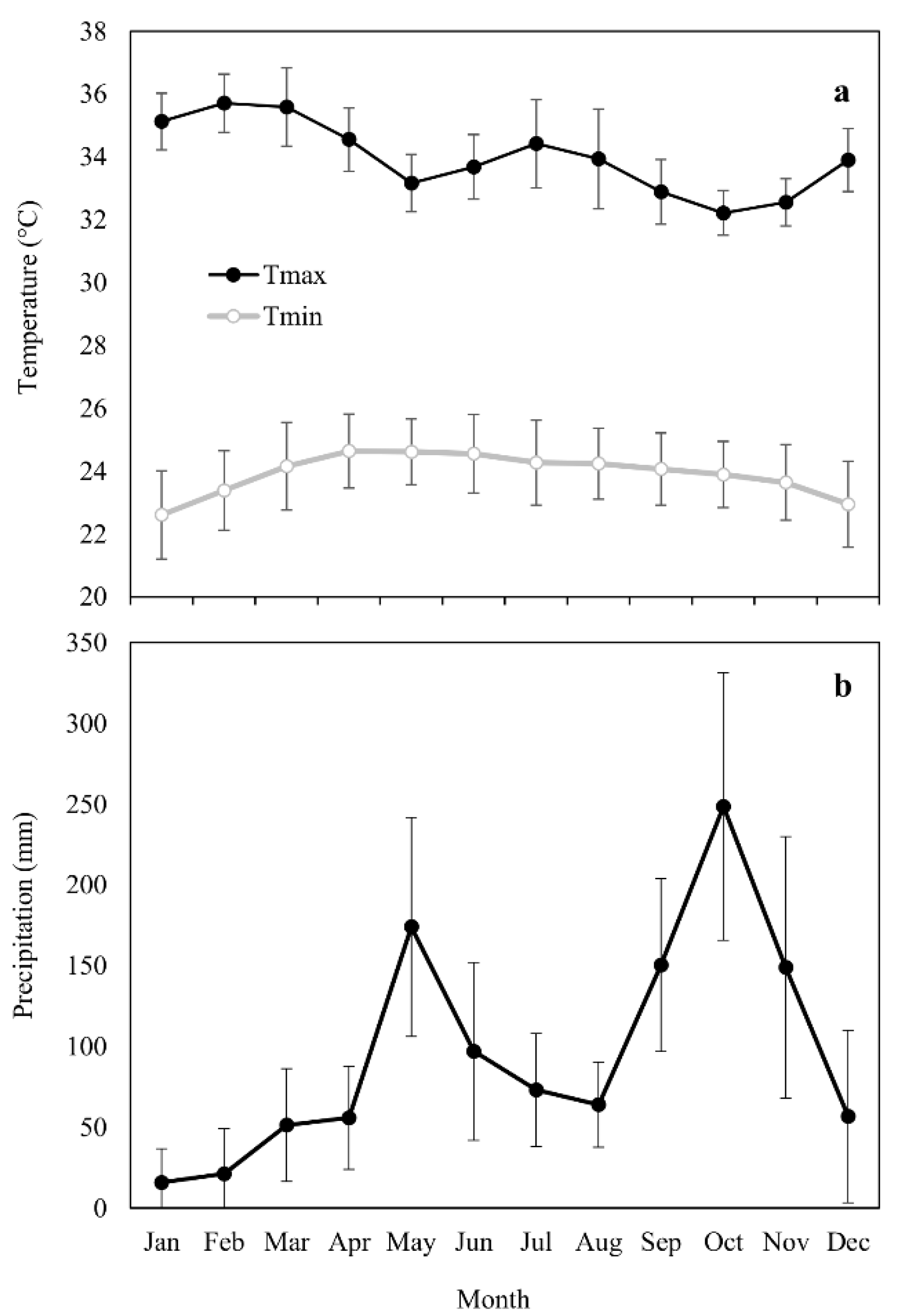
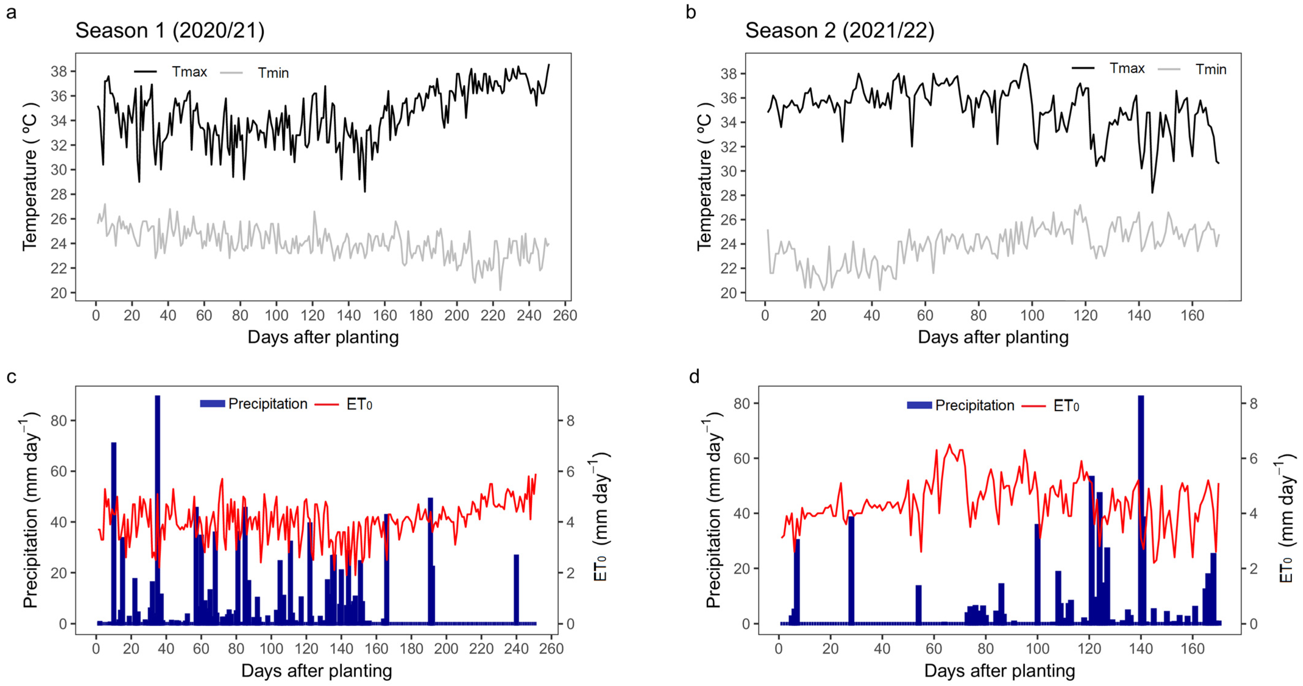
During the crop seasons (2020/21 and 2021/22), information (data) was collected and used as entries to the AquaCrop model.

2.4.1. Climate Data

Meteorological data were obtained from an automatic weather station located in the experimental field. All data were collected at a daily time step. The data comprised average minimum and maximum temperatures (°C), relative humidity (%), total radiation (MJ m−2 day−1), precipitation (mm), wind speed (m s−1), and reference evapotranspiration ET0 (mm day−1). Version 7.0 of the AquaCrop model now calculates reference evapotranspiration by the Penman–Monteith method. The maximum and minimum temperature variation (°C), precipitation (mm), and ET0 (mm) during the two experimental seasons are shown in Figure 2. The precipitation distribution for the two seasons indicated that for season 2020/21 (this was collected over 251 days), it was 1061 mm, while for season 2021/22 (this was collected over 171 days), it was 591 mm. The maximum temperatures oscillated daily between 28 °C and 38 °C for both seasons, and the minimum temperatures oscillated between 20 °C and 27 °C; the cumulative ET0 was 1048 mm and 748 mm in the first and second seasons, respectively.

2.4.2. Crop Data

For each treatment, we observed the crop parameters, such as the growth phase, the seedlings’ emergence date, the maximum canopy cover, the cycle duration (cuts), the time at maximum canopy coverage and to the maximum root, and the minimum and the maximum depth of roots, as well as the canopy growth coefficient (CGC), the crop coefficient for transpiration in the total canopy coverage, and the normalized water productivity (WP*). The upper and lower thresholds for the effect of water stress on canopy expansion, stomatal closure, and early canopy senescence were iteratively adjusted using the independent parameter estimation model (PEST) [35] and considering the minimum and maximum limits recommended for C4 crops by the reference manual for AquaCrop.
The crop phenology was observed in calendar days. The green canopy coverage was monitored twice a week in each treatment taking zenithal photographs of the canopy with a digital camera. We used CobCal Software [36] to analyze canopy cover images.

2.4.3. Soil Data

Before the experiment, a soil profile was excavated at 1 m depth; samples were collected and submitted to the laboratory for analysis. The soil was classified as clay loam, with 72.15% sand, 13.99% silt, 13.86% clay, slightly acidic pH (6.4), and low organic matter content (1.0%). The field capacity (FC) and the permanent wilting point (PWP) were determined by the gravimetric method [37,38]. The FC was 25.3% Vol; the PWP was 8.58% Vol; the hydraulic saturated conductivity (Ks) was 144 mm day−1; and the apparent density average was only 1.58 g cm−3. The soil water content was measured twice a day; we collected four soil samples per treatment at a depth of 15 cm using a soil auger helical; it was also taken before and after each irrigation event. The gravimetric soil water content was determined by the drying method in a furnace, and its value for each treatment was taken from the average of the four experimental units from each level of humidity at the equal sampling depth. Volumetric soil water content was calculated by multiplying the value obtained from the gravimetric method by the apparent soil density. The hydraulic and chemical properties of the soil at the experimental site are shown in Table 2 and Table 3.

2.4.4. Above-Ground Biomass

Above-ground biomass was harvested four times in the first season and three times in the second. The evaluations were initiated with a uniform manual cut at 15 cm of the soil (to reflect the local agricultural practices) on day 116 after planting for the first season and after 84 days for the second season. As from the cut of uniformity, each cycle of sampling/harvesting had an interval of 42 days, approximately. We used the quadrant method of collecting three samples, which were selected randomly, per treatment. Each quadrant was 0.4 m × 0.4 m (area of 0.16 m2), and the total yield forage per hectare was obtained through the dry weight of the sample components, which were weighed in fresh 300 g of vegetative material on a digital scale. The sample was placed in a stove with a circulation of force for 72 h at a temperature of 65 °C until the samples obtained constant weight and were weighed.

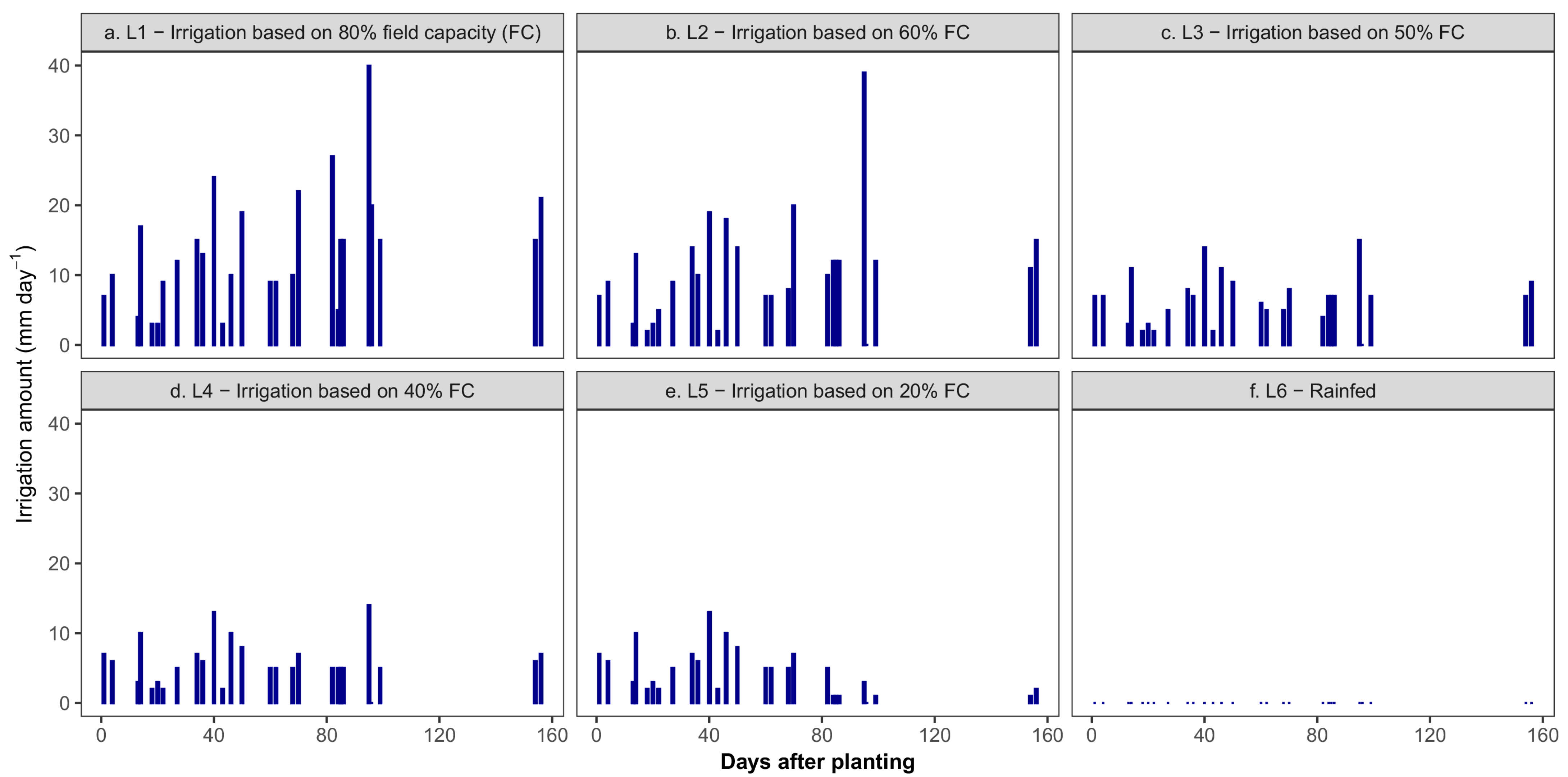
2.4.5. Field Management

An irrigation file was created for each treatment with the quantity of real data of irrigation water applied. In this study, irrigation was carried out according to the daily soil–water balance, using an Excel-based irrigation tool, deciding to irrigate when the depletion level of L1 exceeded 20%. The irrigation application depth was calculated so that L1 reached the field capacity. The irrigation events of the growing seasons are shown in Figure 3 and Figure 4. The field management was established in good conditions of the fertility field, without surface mulches or stress for temperature.

2.5. AquaCrop Model Calibration and Validation

For this study, AquaCrop model version 7.0 [39] was used; this version includes perennial herbaceous forage crops. The calibration was realized through iterations of trial and error as a recommendation by Steduto et al. [30]. The crop growth and field management datasets of L1 from the first season (optimum irrigation conditions) were used for calibration steps. The crop file parameterized for Guinea grass does not exist in the base of the AquaCrop crops database; therefore, it was newly created based on the alfalfa crop file. The model was parameterized for the soil water content, green canopy cover, biomass accumulation, final biomass, and normalized water productivity. The calibrated parameters for the Guinea grass (Megathyrsus maximus cv. Agrosavia sabanera) are indicated in Table 4 and Table 5. The conservative parameters included the canopy growth coefficient (CGC), the canopy declivity coefficient (CDC), the base and upper temperatures, and the thresholds (lower and upper) for the canopy expansion and the stomata closure, as well as the maximum crop coefficient and the normalized water productivity. The non-conservative parameters included seedling density (2 × 10⁶ plants ha−1), maximum canopy coverage (99%), and effective rooting depth (0.36 m). AquaCrop uses growing degree days and calendar days, and this study adopted the mode days of the calendar. The principal phenological stages were observed in detail during the two seasons of growing and were placed directly in an executable crop file of AquaCrop.
In terms of the validation of the model, we realized using the data sets independently obtained treatments L2 to L6 from the first season and L1 to L6 treatments of the second one.
The initial value of the normalized crop water productivity (WP*) of 35.9 g m−2 was obtained as the linear regression of the relation between the biomass accumulation versus the accumulated values of transpiration normalized for ET0, i.e., ∑Tr/ET0 (Figure 5). The WP* value obtained in this study is inside of the established rank for C4 crops in the AquaCrop model. The WP* initial value was adjusted during the biomass calibration; the 35.6 g m−2 value shows a narrow coincidence between the observed biomass, simulated biomass, and the yield, which later was adopted as the WP* for Guinea grass (Megathyrsus maximus cv. Agrosavia sabanera).
Five statistical indices were used to assess how well the AquaCrop model performed in simulating the field-measured parameters during the calibration and validation steps: the Pearson correlation coefficient (R2), Willmott’s index of agreement (d), the root-mean-square error (RMSE), the normalized root-mean-square error (NRMSE), and the Nash–Sutcliffe model efficiency coefficient (Equation (10)).
R 2 = i = 1 n O i O ¯   P i P ¯ i = 1 n O i O ¯ 2 i = 1 n P i P ¯ 2     2
d = 1 i = 1 n P i O i 2 i = 1 n P i O ¯ + O i O ¯ 2
R M S E = i = 1 n P i O i 2 n
N R M S E = 1 O ¯   i = 1 n P i O i 2 n × 100
E F = 1 i = 1 n P i O i 2 i = 1 n O i O ¯ 2
where O i = is the observed data; O ¯ = is the average of observed data; P i = is the simulated data; P ¯ = is the average of simulated data; and n is the number of observations.
The best agreement between the observed and simulated data set for the R2 indicators and d is given when the values are close to 1; values close to 1 indicate perfect model performance. By contrast, RMSE and NRMSE are given the closer the values are to 0. The simulation effect is divided into excellent, good, acceptable, and poor when the NRMSE is minor at 10%, from 10% to 20%, from 20% to 30%, and major at 30%. EF = 1 is optimal and the target value for simulations, while EF = 0 suggests that the model is as precise as the average observed data, and EF < 0 suggests that the average observed data is a better prediction than the model [40,41].

3. Results

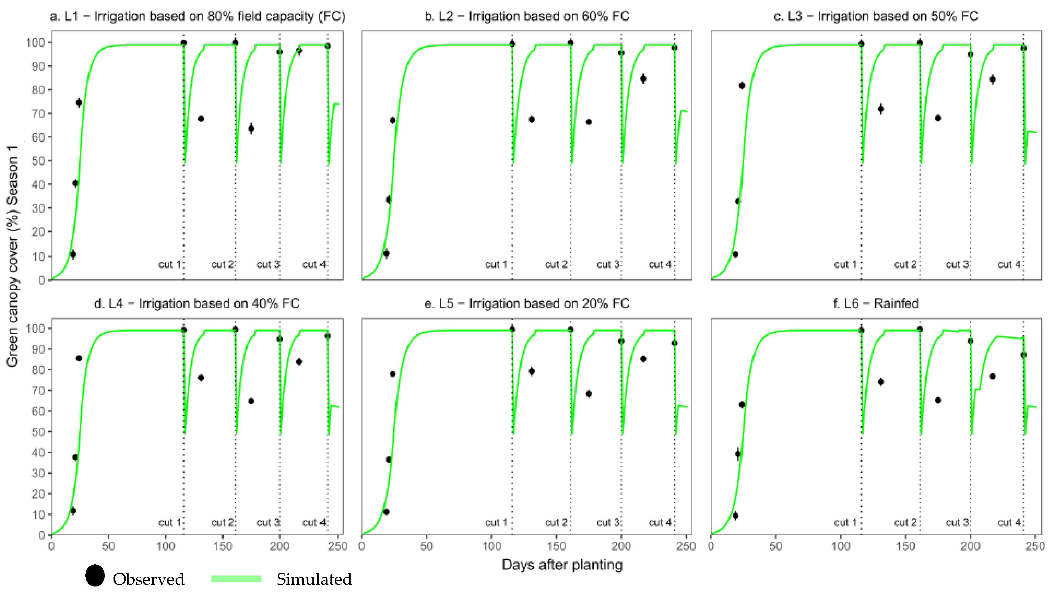
3.1. Canopy Cover (CC)

The canopy coverage evolution (CC) simulated and observed for the six treatments in the calibration and validation seasons showed an appropriate concordance; the CC dynamic throughout the growing season in all the treatments was similar (Figure 6 and Figure 7). AquaCrop achieved capture of the CC development tendency in all the treatments, as it is showing in the acceptable values of R2 (≥0.78), d (≥0.87), and EF (≥0.50) and NRMSE (15.9% ≤ NRMSE ≤ 28.0%) and RMSE (12.0% ≤ RMSE ≤ 18.6%) (Table 6). The simulation precision increased with the decrease in the irrigation level; specifically, the simulation precision in irrigation levels L5 and L6 around 20% of the FC was slightly better than the one from levels L1 to L4. Nevertheless, during the first seasons, the maximum CC was produced appropriately 80 days after seeding in the season 2020/21, which was about five days before the second season in 2021/22.

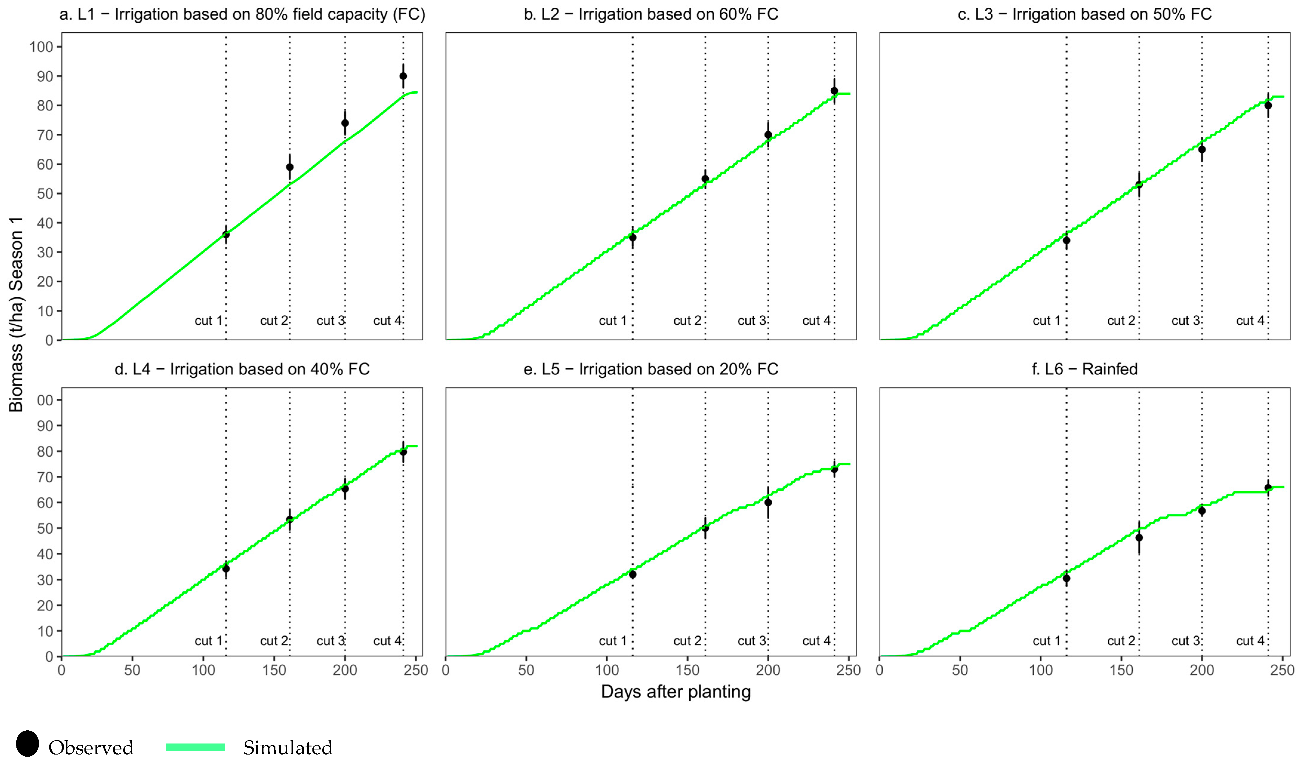
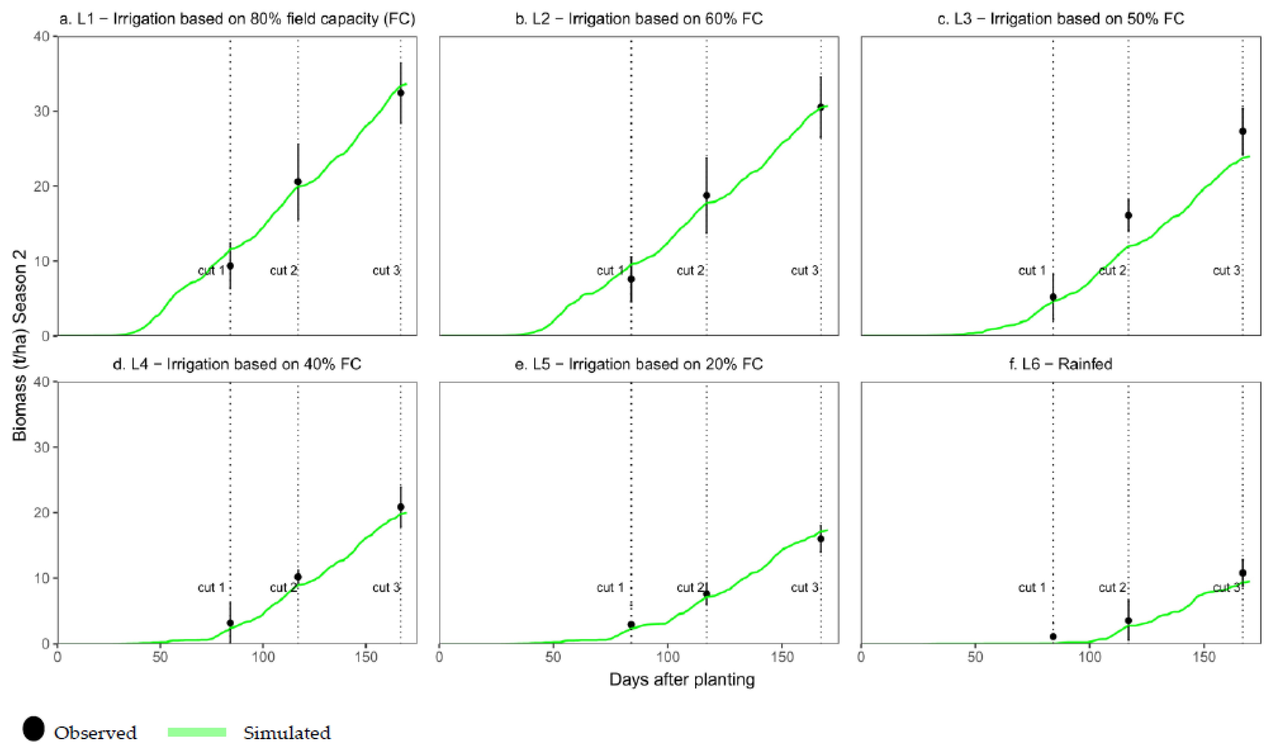
3.2. Cumulative Biomass

Our results show that the AquaCrop performance in the biomass simulation of Guinea grass depends on the level and severity of the stress water experimented on in the crop (Figure 8 and Figure 9). The simulated and actual development of the biomass accumulated in all the treatments was in high agreement with values of R2 ≥ 0.99, d ≥ 0.97, and EF ≥ 0.92, and moderate to poor values of NRMSE (2.5% ≤ NRMSE ≤ 21.9%) and RMSE (0.77 t ha−1 ≤ NRMSE ≤ 5.1 t ha−1). Although the results show satisfactory performance, we observed one slight overestimation systematic in biomass production (1.9–3.6%) in the data set of the first season. This slight overestimation may be due to the errors inherent to field data collection, as they are low and within acceptable levels. In contrast, for the second season data set, the simulated values were underestimated for the higher depletion level treatments (L3, L4, and L6) by the AquaCrop model (9.2–21.2%). This effect was evident in the rainfed treatment because it was a dry season with only one rainfall; this generated the calculation of lower coverages than those observed and, therefore, generated lower biomass estimates than the measures. However, the observed differences are acceptable, and the results are supported by statistical metrics presented in Table 6.

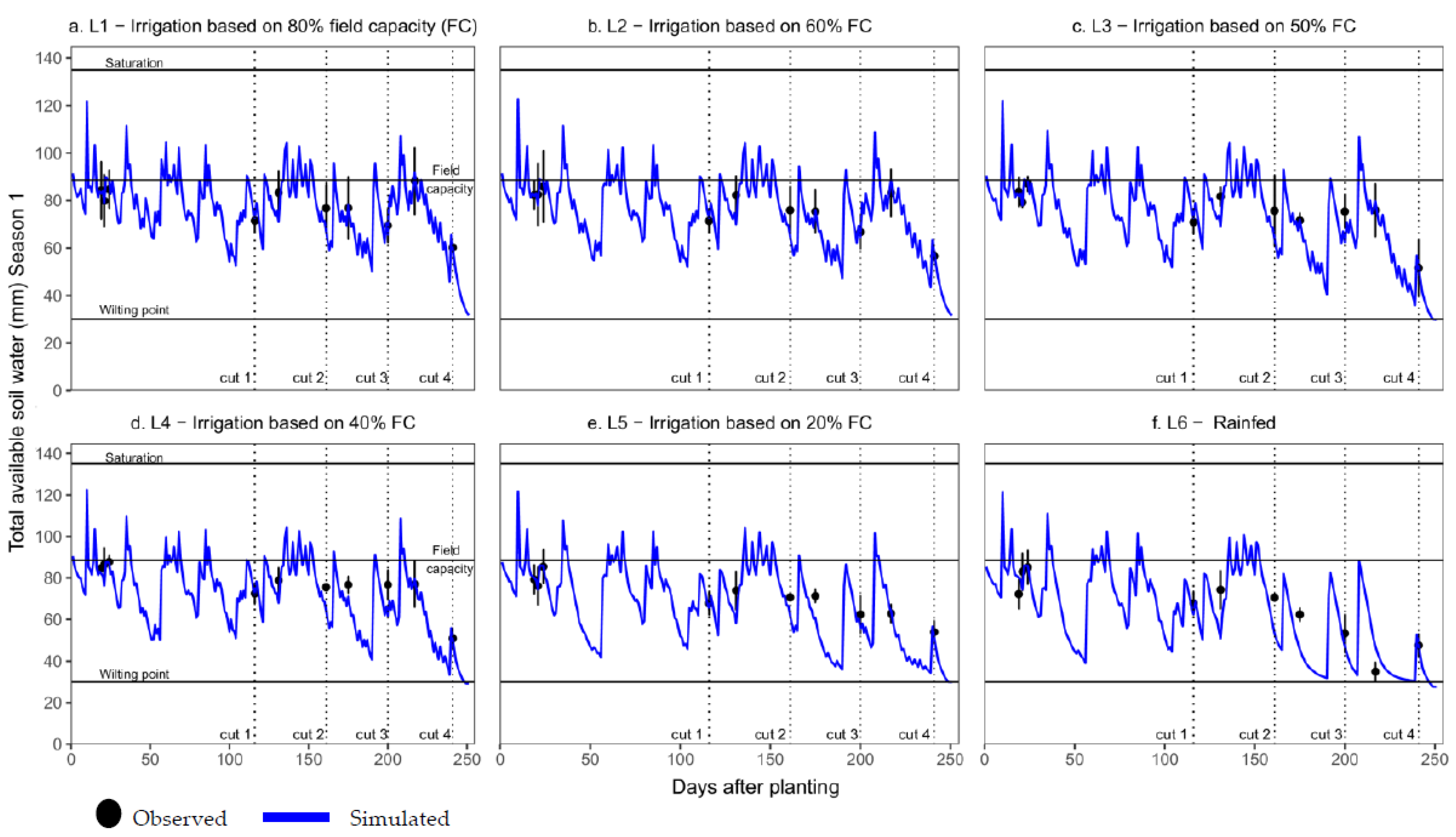
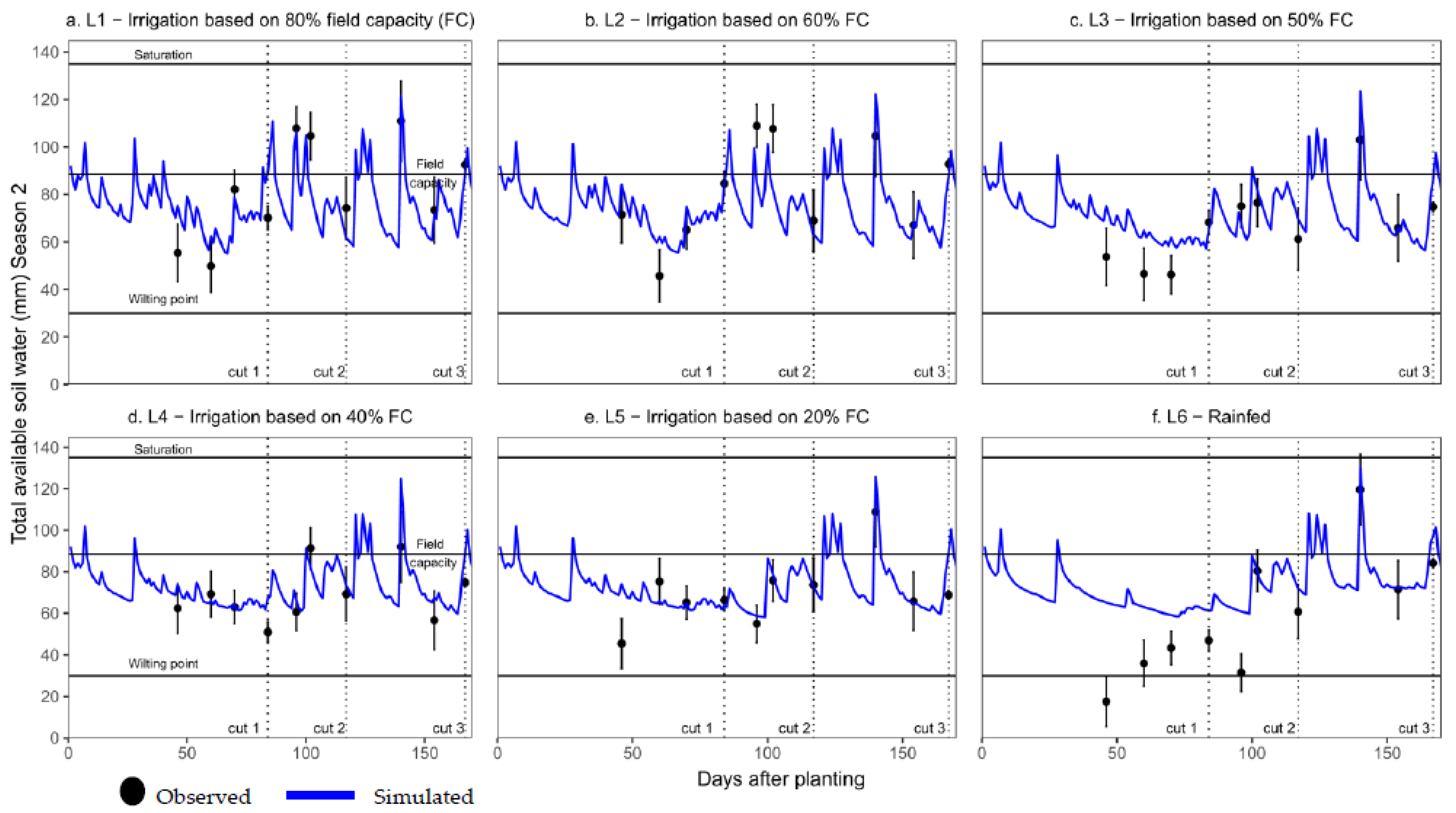
3.3. Soil Water Content

AquaCrop precisely simulated the soil water content observed in the field under variable levels of irrigation, with acceptable values of R2 (≥0.70), d (≥0.79), and EF (≥0.34), and moderate values to poor NRMSE (7.0% ≤ NRMSE ≤ 20.2%) and RMSE (5.4 mm ≤ NRMSE ≤ 14.6 mm) (Table 6). In general, the model had a good performance in the soil water content simulation (TAW) for the calibration and most validation data sets. The simulated values for treatments L1 to L4 during the first season were inside the rank of standard deviation notwithstanding; AquaCrop simulated TAW above the field capacity between the first and second cut of the first season, i.e., between 100–150 DAP (Figure 10). For the second season, during the growth period of treatment L6, the simulated TAW values were overestimated by the model (Figure 11). However, there was water stress in L6 because the observed values reached or exceeded the wilting point level, which could be attributed to low rainfall during this period compared to the first season. This overestimation of TAW occurred mainly in the growth stage of the first cutting and can be explained as the model underestimated canopy cover, which also caused a decrease in calculated transpiration by increasing soil moisture content. In addition, during the second season, AquaCrop did not simulate TAW below the permanent wilting point.
It should be noted that when soil moisture is above FC, the model tends to underestimate TAW, and when soil moisture is below FC, the model tends to overestimate TAW. Similar findings have already been documented in several studies’ experiments evaluating AquaCrop under various irrigation regimes [42,43,44,45,46].

4. Discussion

This study calibrated and validated the AquaCrop model for Guinea grass; the parameters can be adapted for different varieties and agroecological sites using first-grade data, such as biomass, and second-grade data, such as weather, soil, and canopy cover. To our knowledge, this study developed the first calibration and validation of the AquaCrop model for the tropical pasture Megathyrsus maximus.
The AquaCrop model version 7.0 demonstrated efficiency in the Guinea grass growing simulation (Megathyrsus maximus cv. Agrosavia sabanera), managed per cut under different irrigation levels. Guinea grass, as well as other forage gramineous, is tolerant to environmental stress, including drought, soil conditions, shadows [47], and intensive grazing [48]. Our results show an increase in the production of Guinea grass using irrigation to different levels based on field capacity; changes in production aspects when using irrigation have been reported in several studies [49,50]. These reports show that production can increase up to 45%. This capacity can allow many future applications for various tropical pasture species that are important for livestock or energy production from biomass.
In deficit water conditions, the AquaCrop model simulated a rate of canopy expansion that was slower in the initial stages of L4 to L6 treatments from the second growth season, which was also observed on perennial ryegrass and soybeans with a similar conclusion in water stress management treatments [22,23,24,25,26,27,28,29,30,31,32,33,34,35,36,37,38,39,40,41,42,43,44,45,46,47,48,49,50,51]. The observed data simulated with AquaCrop version 7.0 of biomass showed good to very good agreement, reaching statistical results simulated to the best parametrization for available tropical pastures in the literature [12,14,22]. The results obtained in our study regarding the simulation of the final biomass (R2 ≥ 0.99 and d ≥ 0.97) were favorably purchased with those encountered by Araujo et al. [52] and Sousa-Feitosa [21], who simulated Guinea grass using the model APSIM, R2 from 0.75 to 0.87 and d from 0.93 to 0.97, and R2 from 0.64 to 0.93 and d from 0.88 to 0.97, respectively.
The tropical livestock is supported by pasture management, which is the source of more economical nutrients that can be consumed by a ruminant. Our results show the Guinea grass is tolerant (Megathyrsus maximus cv. Agrosavia sabanera) to a wide range of soil humidity. The response of Guinea grass plants to different environmental conditions is a crucial determinant to the establishment of these pastures and can explain the success of the introduced cultivar in the zone. Nevertheless, despite the good results found in the soil water dynamic terms and the crop response in all treatments, it was observed that there were some overestimation problems of TAW during the second season simulations that can be related to sampling errors or specific conditions that occurred during the experiment, which cannot be captured by the model. Although, some authors attribute these discrepancies under limited conditions of soil water to oversimplification of various model components, such as the soil–water balance, root distribution pattern, development and senescence from the canopy, and the biomass partition [53,54,55].
AquaCrop version 7.0 as well as APSIM-Tropical Pasture does not yet simulate the effect of animals trampling and grazing and of the structure and productivity of pasture; therefore, this aspect limits the applicability of the model to estimate the forage available for the animal’s grazed pastures.

5. Conclusions

The grasslands are the source of more affordable nutrients that a ruminant can consume, especially in tropical zones. The AquaCrop model version 7.0 proved to be a promising tool to simulate C4 tropical pastures, such as Guinea grass (Megathyrsus maximus cv. Agrosavia sabanera). This study can be used as reliable guidance to modulate with AquaCrop different strategies of irrigation, variability effects, and the climate change on biomass production of tropical pastures, particularly in South America.
The AquaCrop model could capture several trends of the soil water content, canopy cover, and biomass accumulation related to the effect of the environmental conditions. AquaCrop simulated very well the biomass accumulated at the end in different water regimes. The results of this study provide an important basis for future investigations, including the necessity of parametrization refinement, considering a wider range of environments and tropical grazing variabilities. The data compilation and the enhancement of the biophysical models are essential to allow the analysis of the yield gap and the assessment of climate change impacts on forage production and feeding security. It is suggested that the performance of the AquaCrop model be improved during events of low levels of irrigation or in rainfed conditions.

Author Contributions

Conceptualization, C.A.T.-C.; data curation, C.A.T.-C. and A.V.-A.; formal analysis, C.A.T.-C. and S.M.P.-M.; investigation, C.A.T.-C. and S.M.P.-M.; methodology, C.A.T.-C.; resources, C.A.T.-C.; supervision, C.A.T.-C., S.M.P.-M., and J.E.M.-R.; visualization, S.M.P.-M.; writing—original draft, S.M.P.-M. and C.A.T.-C. All authors have read and agreed to the published version of the manuscript.

Funding

This paper was developed within the framework of the project “Optimización del agua y uso eficiente del suelo para mejorar la producción agropecuaria en escenarios de vulnerabilidad agroclimática del departamento del Cesar”—BPIN 2017000100050—supported by the Colombian Fund for Science, Technology, and Innovation of General System Royalties (FCTeI-SGR), together with Gobernación del Cesar funds.

Institutional Review Board Statement

Not applicable.

Informed Consent Statement

Not applicable.

Data Availability Statement

Not applicable.

Acknowledgments

The authors express their gratitude to all the Centro de Investigación Motilonia -AGROSAVIA (Cesar, Colombia) staff for the logistical and instrumental support provided during the practical development of the work. Likewise, the authors thank the Secretaría de Agricultura y Desarrollo Empresarial of Cesar Department and Prodesarrollo Ltda. We also would like to thank to the anonymous reviewers for their valuable and constructive comments.

Conflicts of Interest

The authors declare no conflict of interest.

References

  1. Bettencourt, E.M.V.; Tilman, M.; Narciso, V.; Da Silva Carvalho, M.L.; de Sousa Henriques, P.D. The Livestock Roles in the Wellbeing of Rural Communities of Timor-Leste. Rev. Econ. Sociol. Rural. 2015, 53, 63–80. [Google Scholar] [CrossRef]
  2. National Administrative Department of Statistics. Cuentas Nacionales. DANE: Bogotá, Colombia, 2022. Available online: https://www.dane.gov.co/index.php/en/30-espanol/cuentas-nacionales (accessed on 26 January 2022).
  3. National Administrative Department of Statistics. Third National Agricultural Census 2014 Colombia. DANE: Bogotá, Colombia, 2022. Available online: https://www.dane.gov.co/index.php/estadisticas-por-tema/agropecuario/censo-nacional-agropecuario-2014#9 (accessed on 26 January 2022).
  4. Moreno-Galván, A.E.; Cortés-Patiño, S.; Romero-Perdomo, F.; Uribe-Vélez, D.; Bashan, Y.; Bonilla, R.R. Proline accumulation and glutathione reductase activity induced by drought-tolerant rhizobacteria as potential mechanisms to alleviate drought stress in Guinea grass. Appl. Soil Ecol. 2020, 147, 103367. [Google Scholar] [CrossRef]
  5. Rhodes, A.C.; Plowes, R.M.; Lawson, J.R.; Gilbert, L.E. Guinea Grass Establishment in South Texas Is Driven by Disturbance History and Savanna Structure. Rangel. Ecol. Manag. 2022, 83, 124–132. [Google Scholar] [CrossRef]
  6. Mojica-Rodríguez, J.E.; Burbano-Erazo, E. Effect of two cultivars of Megathyrsus maximus (Jacq.) on cattle milk production and composition. Pastos Forrajes. 2020, 43, 177–183. [Google Scholar]
  7. Kerguelén, S.L.M.; Solano, L.M.A.; Paternina, E.A.S.; Coronado, J.J.T.; Luquez, J.M.; Rodríguez, L.S.; Mojica, J.E.; Miranda, K.I. Características, Producción y Manejo de la Gramínea Forrajera Tropical Agrosavia Sabanera Para Pastoreo en la Región Caribe Colombiana; Agrosavia: Bogotá, Colombia, 2020. [Google Scholar] [CrossRef]
  8. Sharma, A.; Kumar, V.; Shahzad, B.; Ramakrishnan, M.; Singh Sidhu, G.P.; Bali, A.S.; Handa, N.; Kapoor, D.; Yadav, P.; Khanna, K.; et al. Photosynthetic Response of Plants Under Different Abiotic Stresses: A Review. J. Plant Growth Regul. 2019, 39, 509–531. [Google Scholar] [CrossRef]
  9. Tapia-Coronado, J.J.; Atencio-Solano, L.M.; Mejía-Kerguelen, S.L.; Paternina-Paternina, Y.; Cadena-Torres, J. Evaluación del potencial productivo de nuevas gramíneas forrajeras para las sabanas secas del Caribe en Colombia. Agron. Costarric. 2019, 43, 43–60. [Google Scholar] [CrossRef]
  10. Berauer, B.J.; Wilfahrt, P.A.; Reu, B.; Schuchardt, M.A.; Garcia-Franco, N.; Zistl-Schlingmann, M.; Dannenmann, M.; Kiese, R.; Kühnel, A.M.; Jentsch, A. Predicting forage quality of species-rich pasture grasslands using vis-NIRS to reveal effects of management intensity and climate change. Agric. Ecosyst. Environ. 2020, 296, 106929. [Google Scholar] [CrossRef]
  11. Richards, M.; Arslan, A.; Cavatassi, R.; Rosenstock, T. Climate Change Mitigation Potential of Agricultural Practices Supported by IFAD Investments: An Ex Ante Analysis; IFAD Research Series; IFAD: Rome, Italy, 2019; pp. 1–30. Available online: https://cgspace.cgiar.org/handle/10568/100166 (accessed on 10 October 2022).
  12. Pequeno, D.N.L.; Pedreira, C.G.S.; Boote, K.J.; Alderman, P.D.; Faria, A.F.G. Species-genotypic parameters of the CROPGRO Perennial Forage Model: Implications for comparison of three tropical pasture grasses. Grass Forage Sci. 2017, 73, 440–455. [Google Scholar] [CrossRef]
  13. Bana, R.S.; Bamboriya, S.D.; Padaria, R.N.; Dhakar, R.K.; Khaswan, S.L.; Choudhary, R.L.; Bamboriya, J.S. Planting Period Effects on Wheat Productivity and Water Footprints: Insights through Adaptive Trials and APSIM Simulations. Agronomy 2022, 12, 226. [Google Scholar] [CrossRef]
  14. Andrade, A.S.; Santos, P.M.; Pezzopane, J.R.M.; de Araujo, L.C.; Pedreira, B.C.; Pedreira, C.G.S.; Marin, F.R.; Lara, M.A.S. Simulating tropical forage growth and biomass accumulation: An overview of model development and application. Grass Forage Sci. 2015, 71, 54–65. [Google Scholar] [CrossRef] [Green Version]
  15. Kiniry, J.R.; Burson, B.L.; Evers, G.W.; Williams, J.R.; Sanchez, H.; Wade, C.; Featherston, J.W.; Greenwade, J. Coastal Bermudagrass, Bahiagrass, and Native Range Simulation at Diverse Sites in Texas. Agron. J. 2007, 99, 450–461. [Google Scholar] [CrossRef] [Green Version]
  16. Ojeda, J.J.; Volenec, J.J.; Brouder, S.M.; Caviglia, O.P.; Agnusdei, M.G. Evaluation of Agricultural Production Systems Simulator as yield predictor of Panicum virgatumand Miscanthusxgiganteusin several US environments. GCB Bioenergy 2016, 9, 796–816. [Google Scholar] [CrossRef]
  17. Bosi, C.; Sentelhas, P.C.; Pezzopane, J.R.M.; Santos, P.M. CROPGRO-Perennial Forage model parameterization for simulating Piatã palisade grass growth in monoculture and in a silvopastoral system. Agric. Syst. 2020, 177, 102724. [Google Scholar] [CrossRef]
  18. dos Santos, M.L.; Santos, P.M.; Boote, K.J.; Pequeno, D.N.L.; Barioni, L.G.; Cuadra, S.V.; Hoogenboom, G. Applying the CROPGRO Perennial Forage Model for long-term estimates of Marandu palisadegrass production in livestock management scenarios in Brazil. Field Crops Res. 2022, 286, 108629. [Google Scholar] [CrossRef]
  19. Bosi, C.; Sentelhas, P.C.; Huth, N.I.; Pezzopane, J.R.M.; Andreucci, M.P.; Santos, P.M. APSIM-Tropical Pasture: A model for simulating perennial tropical grass growth and its parameterisation for palisade grass (Brachiaria brizantha). Agric. Syst. 2020, 184, 102917. [Google Scholar] [CrossRef]
  20. Gomes, F.J.; Bosi, C.; Pedreira, B.C.; Santos, P.M.; Pedreira, C.G.S. Parameterization of the APSIM model for simulating palisadegrass growth under continuous stocking in monoculture and in a silvopastoral system. Agric. Syst. 2020, 184, 102876. [Google Scholar] [CrossRef]
  21. Sousa-Feitosa, T. Parametrização do Modelo APSIM-Tropical Pasture Para a Simulação de Crescimento de Megathyrsus maximus cv. Mombaça. Ph.D. Thesis, Universidade de São Paulo, São Paulo, Brasil, 2021. Available online: https://www.teses.usp.br/teses/disponiveis/11/11139/tde-14092021-163128/publico/Tiberio_Sousa_Feitosa_versao_revisada.pdf (accessed on 3 November 2022).
  22. Terán-Chaves, C.A.; García-Prats, A.; Polo-Murcia, S.M. Calibration and Validation of the FAO AquaCrop Water Productivity Model for Perennial Ryegrass (Lolium perenne L.). Water 2022, 14, 3933. [Google Scholar] [CrossRef]
  23. Terán-Chaves, C.A. Determinación de la Huella Hídrica y Modelación de la Producción de Biomasa de Cultivos Forrajeros a Partir del Agua en la Sabana de Bogotá (Colombia). Ph.D. Thesis, Universitat Politècnica de València, Valencia, Spain, 2015. [Google Scholar] [CrossRef] [Green Version]
  24. Wellens, J.; Raes, D.; Fereres, E.; Diels, J.; Coppye, C.; Adiele, J.G.; Ezui, K.S.G.; Becerra, L.A.; Selvaraj, M.G.; Dercon, G.; et al. Calibration and validation of the FAO AquaCrop water productivity model for cassava (Manihot esculenta Crantz). Agric. Water Manag. 2022, 263, 107491. [Google Scholar] [CrossRef]
  25. Raes, D.; Steduto, P.; Hsiao, T.C.; Fereres, E. AquaCrop—The FAO Crop Model to Simulate Yield Response to Water: II. Main Algorithms and Software Description. Agron. J. 2009, 101, 438–447. [Google Scholar] [CrossRef] [Green Version]
  26. Raes, D. AquaCrop Training Handbooks Book II.—Running AquaCrop; Food and Agriculture Organization of the United Nations: Rome, Italy, 2022; Available online: https://www.fao.org/3/i6052en/i6052en.pdf (accessed on 17 October 2022).
  27. Terán-Chaves, C.A.; Duarte-Carvajalino, J.M.; Polo-Murcia, S. Quality control and filling of daily temperature and precipitation time series in Colombia. Meteorol. Z. 2021, 30, 489–501. [Google Scholar] [CrossRef]
  28. Uzcátegui-Varela, J.P.; Chompre, K.; Castillo, D.; Rangel, S.; Briceño-Rangel, A.; Piña, A. Nutritional assessment of tropical pastures as a sustainability strategy in dual-purpose cattle ranching in the South of Lake Maracaibo, Venezuela. J. Saudi Soc. Agric. Sci. 2022, 21, 432–439. [Google Scholar] [CrossRef]
  29. Hanks, R.J.; Keller, J.; Rasmussen, V.P.; Wilson, G.D. Line source sprinkler for continuous variable irrigation-crop production studies. Soil Sci. Soc. Am. J. 1976, 40, 426–429. [Google Scholar] [CrossRef]
  30. Steduto, P.; Hsiao, T.C.; Raes, D.; Fereres, E. AquaCrop-The FAO Crop Model to Simulate Yield Response to Water: I. Concepts and Underlying Principles. Agron. J. 2009, 101, 426–437. [Google Scholar] [CrossRef] [Green Version]
  31. Steduto, P.; Hsiao, T.C.; Fereres, E. On the conservative behavior of biomass water productivity. Irrig. Sci. 2007, 25, 189–207. [Google Scholar] [CrossRef] [Green Version]
  32. Allen, R.G.; Pereira, L.S.; Raes, D.; Smith, M. FAO Irrigation and Drainage Paper No. 56—Crop Evapotranspiration; FAO: Rome, Italy, 1998; Available online: www.climasouth.eu/sites/default/files/FAO%2056.pdf (accessed on 13 August 2022).
  33. Hsiao, T.C.; Fereres, E.; Steduto, P.; Raes, D. AquaCrop parameterization, calibration, and validation guide. Crop Yield Response to Water. In FAO Irrigation and Drainage Paper, 66; Food and Agriculture Organization of the United Nations: Rome, Italy, 2012; pp. 70–87. [Google Scholar]
  34. Hisao, T.; Fereres, E.; Steduto, P.; Raes, D. AquaCrop Version 7.0. Chapter 4 Calibration Guidance; Food and Agriculture Organization of the United Nations, Land and Water Division: Rome, Italy, 2022; Available online: https://www.fao.org/3/br249e/br249e.pdf (accessed on 3 October 2022).
  35. Doherty, J. PEST: Model Independent Parameter Estimation, User Manual, 5th ed.; Watermark Numerical Computing: Brisbane, Australia, 2005; Available online: https://pesthomepage.org/ (accessed on 8 December 2022).
  36. Ferrari, H.; Ferrari, C.; Ferrari, F. CobCal; Version 2.1; Instituto Nacional de Tecnología Agropecuaria: Entre Ríos, Argentina, 2006; Available online: https://www.cobcal.com.ar (accessed on 3 October 2022).
  37. Klute, A. Water Retention: Laboratory Methods. In Methods of Soil Analysis; Part 1—Physical and Mineralogical Methods, 2nd ed.; SSSA Book Series; ASA & SSSA: Madison, WI, USA, 1986; pp. 635–662. [Google Scholar]
  38. Taylor, S.A.; Ashcroft, G.L. Physical edaphology. In The Physics of Irrigated and Non-Irrigated Soils, 1st ed.; Utah State University: Logan, UT, USA, 1972; p. 303. Available online: cabdirect.or (accessed on 1 January 2022).
  39. AquaCrop Stand-Alone (Plug-In) Program; Version 7.0; Food and Agriculture Organization of the United Nations, Land and Water Division: Rome, Italy, 2022; Available online: https://www.fao.org/aquacrop/software/aquacropplug-inprogramme/en/ (accessed on 3 October 2022).
  40. Cheng, M.; Wang, H.; Fan, J.; Xiang, Y.; Liu, X.; Liao, Z.; Abdelghany, A.E.; Zhang, F.; Li, Z. Evaluation of AquaCrop model for greenhouse cherry tomato with plastic film mulch under various water and nitrogen supplies. Agric. Water Manag. 2022, 274, 107949. [Google Scholar] [CrossRef]
  41. Raes, D.; Steduto, P.; Hisao, T.; Fereres, E. Reference Manual, Chapter 2- AquaCrop, Version 7.0; Food and Agriculture Organization of the United Nations, Land and Water Division: Rome, Italy, 2022; pp. 283–287. Available online: https://www.fao.org/3/br267e/br267e.pdf (accessed on 2 December 2022).
  42. Er-Raki, S.; Bouras, E.H.; Rodriguez, J.L.; Watts, C.; Lizárraga-Celaya, C.; Chehbouni, A. Parameterization of the AquaCrop model for simulating table grapes growth and water productivity in an arid region of Mexico. Agric. Water Manag. 2021, 245, 106585. [Google Scholar] [CrossRef]
  43. Adeboye, O.B.; Schultz, B.; Adekalu, K.O.; Prasad, K. Performance evaluation of AquaCrop in simulating soil water storage, yield, and water productivity of rainfed soybeans (Glycine max L. merr) in Ile-Ife, Nigeria. Agric. Water Manag. 2019, 213, 11301146. [Google Scholar] [CrossRef]
  44. Kale, S.; Madenoğlu, S. Evaluating AquaCrop Model for Winter Wheat under Various Irrigation Conditions in Turkey. Tarim Bilim. Derg. 2018, 24, 205–217. [Google Scholar] [CrossRef] [Green Version]
  45. Toumi, J.; Er-Raki, S.; Ezzahar, J.; Khabba, S.; Jarlan, L.; Chehbouni, A. Performance assessment of AquaCrop model for estimating evapotranspiration, soil water content and grain yield of winter wheat in Tensift Al Haouz (Morocco): Application to irrigation management. Agric. Water Manag. 2016, 163, 219–235. [Google Scholar] [CrossRef]
  46. Farahani, H.; Izzi, G.; Oweis, T. Parameterization and Evaluation of the AquaCrop Model for Full and Deficit Irrigated Cotton. Agron. J. 2009, 101, 469–476. [Google Scholar] [CrossRef] [Green Version]
  47. Malaviya, D.R.; Baig, M.J.; Kumar, B.; Kaushal, P. Effects of shade on guinea grass genotypes Megathyrsus maximus (Poales: Poaceae). Rev. Biol. Trop. 2020, 68, 563–572. [Google Scholar] [CrossRef]
  48. Benabderrahim, M.A.; Elfalleh, W. Forage Potential of Non-Native Guinea Grass in North African Agroecosystems: Genetic, Agronomic, and Adaptive Traits. Agronomy 2021, 11, 1071. [Google Scholar] [CrossRef]
  49. Habermann, E.; Dias de Oliveira, E.A.; Contin, D.R.; Delvecchio, G.; Viciedo, D.O.; de Moraes, M.A.; de Mello Prado, R.; de Pinho Costa, K.A.; Braga, M.R.; Martinez, C.A. Warming and water deficit impact leaf photosynthesis and decrease forage quality and digestibility of a C4 tropical grass. Physiol. Plant 2019, 165, 383–402. [Google Scholar] [CrossRef]
  50. Antoniel, L.S.; Prado, G.D.; Tinos, A.C.; Beltrame, G.A.; Almeida, J.V.C.D.; Cuco, G.P. Pasture production under different irrigation depths. Rev. Bras. Eng. Agricola Ambient. 2016, 20, 539–544. [Google Scholar] [CrossRef] [Green Version]
  51. Paredes, P.; Wei, Z.; Liu, Y.; Xu, D.; Xin, Y.; Zhang, B.; Pereira, L. Performance assessment of the FAO AquaCrop model for soil water, soil evaporation, biomass and yield of soybeans in North China Plain. Agric. Water Manag. 2015, 152, 57–71. [Google Scholar] [CrossRef] [Green Version]
  52. Araujo, L.C.; Santos, P.M.; Rodriguez, D.; Pezzopane, J.R.M.; Oliveira, P.P.; Cruz, P.G. Simulating Guinea grass production: Empirical and mechanistic approaches. Agron. J. 2013, 105, 61–69. [Google Scholar] [CrossRef] [Green Version]
  53. Ahmadi, S.H.; Mosallaeepour, E.; Kamgar-Haghighi, A.A.; Sepaskhah, A.R. Modeling Maize Yield and Soil Water Content with AquaCrop Under Full and Deficit Irrigation Managements. Water Resour. Manag. 2015, 29, 2837–2853. [Google Scholar] [CrossRef]
  54. Tan, S.; Wang, Q.; Zhang, J.; Chen, Y.; Shan, Y.; Xu, D. Performance of AquaCrop model for cotton growth simulation under film-mulched drip irrigation in southern Xinjiang, China. Agric. Water Manag. 2018, 196, 99–113. [Google Scholar] [CrossRef]
  55. Ran, H.; Kang, S.; Li, F.; Du, T.; Tong, L.; Li, S.; Ding, R.; Zhang, X. Parameterization of the AquaCrop model for full and deficit irrigated maize for seed production in arid Northwest China. Agric. Water Manag. 2018, 203, 438–450. [Google Scholar] [CrossRef]
Figure 1. Long-term (1980–2019) mean monthly (a) maximum (Tmax) and minimum (Tmin) temperatures and (b) precipitation amounts in the Motilonia Research Center of Agrosavia (Cesar, Colombia). Error bars represent standard deviation.
Water 15 00863 g001
Figure 2. Daily weather data during the experiment for calibration and validation of the AquaCrop model for Megathyrsus maximus cv. Agrosavia sabanera at the Motilonia Research Center (Cesar, Colombia), season 1 from 19 June 2020 to 24 February 2021 and season 2 from 17 December 2021 to 4 June 2022. (a) Tmin and Tmax are the minimum and the maximum of daily air temperature in season 1; (b) Tmin and Tmax are the minimum and the maximum of daily air temperature in season 2; (c) Precipitation and reference evapotranspiration (ET0) in season 1; (d) Precipitation and reference evapotranspiration (ET0) in season 2.
Water 15 00863 g002
Figure 3. Detailed irrigation schedule for the different treatments during the Guinea grass (Megathyrsus maximus cv. Agrosavia sabanera) first growing season (from 19 June 2020 to 24 February 2021). (a). Irrigation schedule for the treatment L1—irrigation based on 80% field capacity (FC); (b). Irrigation schedule for the treatment L2—irrigation based on 60% FC; (c) Irrigation schedule for the treatment L3—irrigation based on 50% FC; (d) Irrigation schedule for the treatment L4—irrigation based on 40% FC; (e) Irrigation schedule for the treatment L5—irrigation based on 20% FC; (f) Irrigation schedule for the treatment L6—rainfed.
Water 15 00863 g003
Figure 4. Detailed irrigation schedule for the different treatments during the Guinea grass (Megathyrsus maximus cv. Agrosavia sabanera) second growing season (from 17 December 2021 to 4 June 2022). (a). Irrigation schedule for the treatment L1—irrigation based on 80% field capacity (FC); (b). Irrigation schedule for the treatment L2—irrigation based on 60% FC; (c) Irrigation schedule for the treatment L3—irrigation based on 50% FC; (d) Irrigation schedule for the treatment L4—irrigation based on 40% FC; (e) Irrigation schedule for the treatment L5—irrigation based on 20% FC; (f) Irrigation schedule for the treatment L6—rainfed.
Water 15 00863 g004
Figure 5. Cumulative biomass and cumulative transpiration (normalized for ET0 and CO2) for the Guinea grass (Megathyrsus maximus cv. Agrosavia sabanera) fields (black dots). The black line represents the WP* of 35.93 g m2.
Water 15 00863 g005
Figure 6. Observed and simulated canopy cover (CC) under different irrigation treatments during the first growing season (2020/21) of Guinea grass (Megathyrsus maximus cv. Agrosavia sabanera). The error bars represent standard deviations. (a). CC for the treatment L1—irrigation based on 80% field capacity (FC); (b). CC for the treatment L2—irrigation based on 60% FC; (c) CC for the treatment L3—irrigation based on 50% FC; (d) CC for the treatment L4—irrigation based on 40% FC; (e) CC for the treatment L5—irrigation based on 20% FC; (f) CC for the treatment L6—rainfed.
Water 15 00863 g006
Figure 7. Observed and simulated canopy cover (CC) under different irrigation treatments during the second growing season (2021/22) of Guinea grass (Megathyrsus maximus cv. Agrosavia sabanera). The error bars represent standard deviations. (a). CC for the treatment L1—irrigation based on 80% field capacity (FC); (b). CC for the treatment L2—irrigation based on 60% FC; (c) CC for the treatment L3—irrigation based on 50% FC; (d) CC for the treatment L4—irrigation based on 40% FC; (e) CC for the treatment L5—irrigation based on 20% FC; (f) CC for the treatment L6—rainfed.
Water 15 00863 g007
Figure 8. Observed and simulated cumulative biomass under different irrigation treatments during the first growing season (2020/21) of Guinea grass (Megathyrsus maximus cv. Agrosavia sabanera). The error bars represent standard deviations. (a). Cumulative biomass for the treatment L1—irrigation based on 80% field capacity (FC); (b). Cumulative biomass for the treatment L2—irrigation based on 60% FC; (c) Cumulative biomass for the treatment L3—irrigation based on 50% FC; (d) Cumulative biomass for the treatment L4—irrigation based on 40% FC; (e) Cumulative biomass for the treatment L5—irrigation based on 20% FC; (f) Cumulative biomass for the treatment L6—rainfed.
Water 15 00863 g008
Figure 9. Observed and simulated cumulative biomass under different irrigation treatments during the second growing season (2021/22) of Guinea grass (Megathyrsus maximus cv. Agrosavia sabanera). The error bars represent standard deviations. (a). Cumulative biomass for the treatment L1—irrigation based on 80% field capacity (FC); (b). Cumulative biomass for the treatment L2—irrigation based on 60% FC; (c) Cumulative biomass for the treatment L3—irrigation based on 50% FC; (d) Cumulative biomass for the treatment L4—irrigation based on 40% FC; (e) Cumulative biomass for the treatment L5—irrigation based on 20% FC; (f) Cumulative biomass for the treatment L6—rainfed.
Water 15 00863 g009
Figure 10. Observed and simulated total available soil water (TAW) under different irrigation treatments during the first growing season (2020/21) of Guinea grass (Megathyrsus maximus cv. Agrosavia sabanera). The error bars represent standard deviations. (a). TAW for the treatment L1—irrigation based on 80% field capacity (FC); (b). TAW for the treatment L2—irrigation based on 60% FC; (c) TAW for the treatment L3—irrigation based on 50% FC; (d) TAW for the treatment L4—irrigation based on 40% FC; (e) TAW for the treatment L5—irrigation based on 20% FC; (f) TAW for the treatment L6—rainfed.
Water 15 00863 g010
Figure 11. Observed and simulated total available soil water (TAW) under different irrigation treatments during the second growing season (2021/22) of Guinea grass (Megathyrsus maximus cv. Agrosavia sabanera). The error bars represent standard deviations. (a). TAW for the treatment L1—irrigation based on 80% field capacity (FC); (b). TAW for the treatment L2—irrigation based on 60% FC; (c) TAW for the treatment L3—irrigation based on 50% FC; (d) TAW for the treatment L4—irrigation based on 40% FC; (e) TAW for the treatment L5—irrigation based on 20% FC; (f) TAW for the treatment L6—rainfed.
Water 15 00863 g011
Table 1. Time and doses of fertilizer applications during the experiment.
Fertilizer1st Application (15DAE)2nd Application (30DAE)3rd Application (45DAE)
kg ha−1
Nitrogen (N)415549
Phosphorus (P2O5)393926
Potassium (K2O)515134
Magnesium (MgSO4.7H2O) 4.54.5
Table 2. Hydraulic properties of the soil at the experimental field.
Depth (m)θFC
(mm m−1)
θPWP
(mm m−1)
θsat
(mm m−1)
Ks
(mm day−1)
Sand
(%)
Silt
(%)
Clay
(%)
0.35253.085.846014472.1513.9913.86
Notes: θFC = water content at field capacity, θPWP = water content at wilting point, θsat = water content at saturation, Ks = saturated hydraulic conductivity.
Table 3. Chemical properties of the soil at the experimental field.
Depth (m)pHEC (dS m−1) Available N
(mg kg−1)
Available P
(mg kg−1)
Available K
(mg kg−1)
Organic Carbon (%)
0.206.40.714601441580.55
Notes: EC = Soil electrical conductivity.
Table 4. Conservative parameters used in calibrating and validating the model for simulating the response of Guinea grass (Megathyrsus maximus cv. Agrosavia sabanera) under different water regimes.
Crop ParameterValueMethod of
Determination
Base temperature (°C)11.2L
Upper temperature (°C)43.5L
Soil water depletion factor for canopy expansion (p-exp)–Upper threshold0.25E
Soil water depletion factor for canopy expansion (p-exp)–Lower threshold1.00E
Shape factor for water stress coefficient for canopy expansion10.7E
Soil water depletion fraction for stomatal control (p-sto)–Upper threshold0.5E
Shape factor for water stress coefficient for stomatal control4.1E
Soil water depletion factor for canopy senescence (p-sen)–Upper threshold0.85E
Shape factor for water stress coefficient for canopy senescence3.0E
vol% for Anaerobiotic point (SAT–[vol%]) at which deficient aeration occurs−2D
Canopy growth coefficient (CGC): Increase in canopy cover (fraction of soil cover per day)0.1686 M
Canopy decline coefficient (CDC): Decrease in canopy cover (in fraction per day)0.0123E
Crop coefficient when canopy is complete but prior to senescence (Kc, Tr, x)1.12M
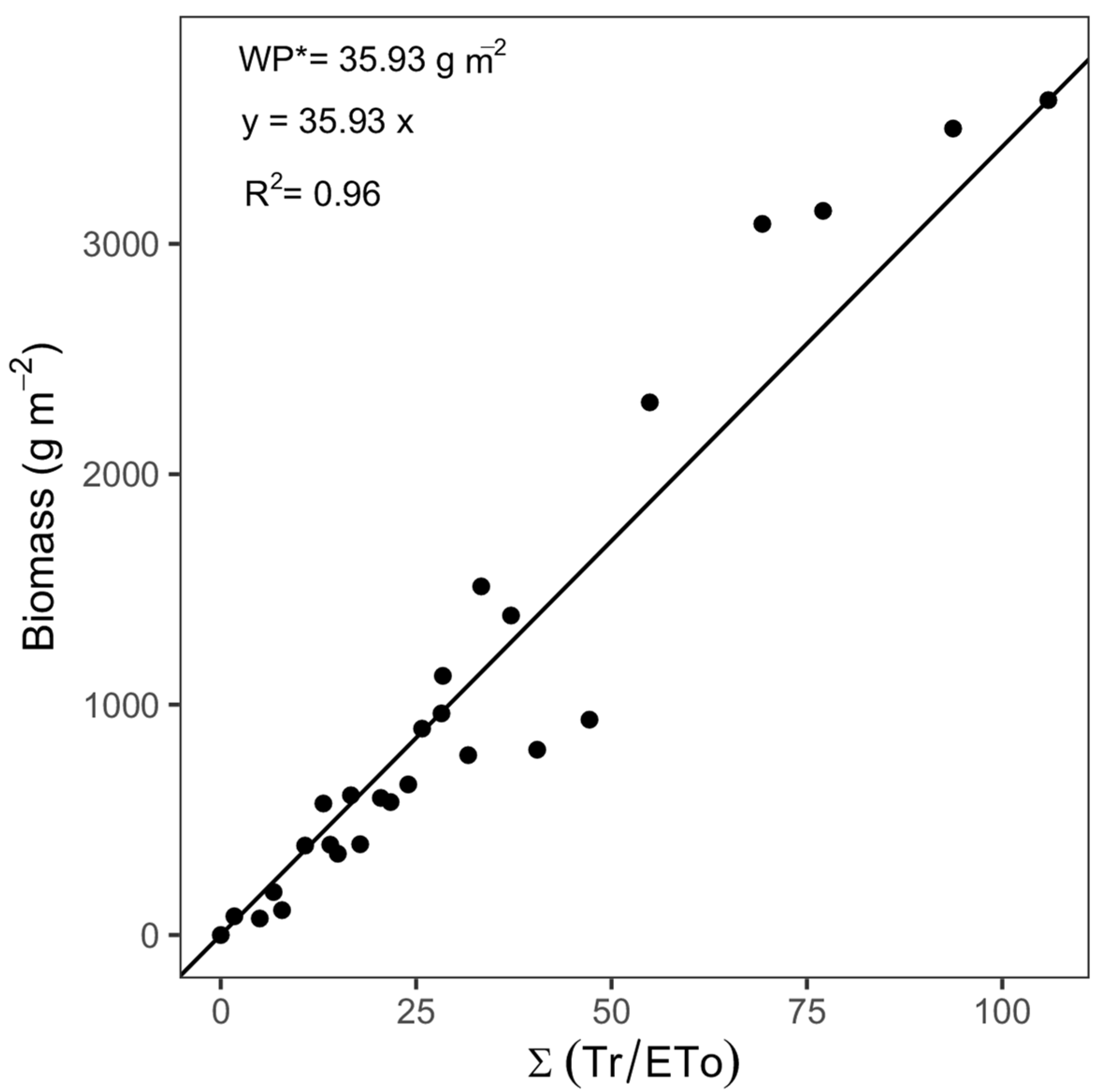
Normalized Water Productivity for ET0 and CO2 (WP*) (g m−2)35.6C
Notes: C: calibration; D: AquaCrop default; E: estimation; L: literature; M: measured.
Table 5. Non-conservative parameters used in calibrating and validating the model for simulating the response of Guinea grass (Megathyrsus maximus cv. Agrosavia sabanera) under different water regimes.
Crop ParameterValueMethod of
Determination
Time to reach 90% crop emergence [days] for the first cut8M
Time to reach 90% crop emergence [days] after the first cutting1M
Calendar Days from sowing to maximum rooting depth60M
Calendar days from sowing to flowering [days]0D
Calendar days from sowing to flowering [days] after the first cutting0D
Calendar days from sowing to maturity (length of crop cycle) for the first cut 90C
Calendar days from sowing to maturity (length of crop cycle) after the first cutting42C
Minimum effective rooting depth (m)0.04M
Maximum effective rooting depth (m)0.36M
Shape factor describing root zone expansion15M
Maximum root water extraction (m³ water/m³ soil day) in the top quarter of root zone0.030E
Maximum root water extraction (m³ water/m³ soil day) in the bottom quarter of root zone0.020E
Effect of canopy cover in reducing soil evaporation in late season stage50E
Soil surface covered by an individual seedling at 90% emergence (cm²) first cut0.35M
Soil surface covered by an individual seedling at 90% emergence (cm²) after the first cutting8.76M
Number of plants per hectare2,001,100M
Number of plants per m²200.1M
Maximum canopy cover (CCx) in fraction soil cover0.99M
Reference Harvest Index (HIo) (%)100D
Notes: C: calibration; D: AquaCrop default; E: estimation; M: measured.
Table 6. Statistical indicators of green canopy cover, cumulative biomass, and total available soil water simulated by AquaCrop (calibration and validation) under different treatments in two growing seasons (2020/21 and 2021/22) of Guinea grass (Megathyrsus maximus cv. Agrosavia sabanera).
StatisticsCalibration Season 1 (2020/21)Validation Season 1 (2020/21)Validation Season 2 (2021/22)
L1L2L3L4L5L6L1L2L3L4L5L6
Green Canopy Cover (%)
R20.840.880.840.820.870.890.800.780.880.880.910.97
d0.910.930.910.900.920.930.820.870.900.920.940.97
RMSE (%)17.4015.7017.5018.6016.1015.7013.6014.1013.7015.9014.7012.00
NRMSE (%)23.2021.8023.6024.9021.6022.2015.9017.0017.1023.3025.0028.00
EF0.630.700.630.550.660.660.500.520.470.600.760.87
Cumulative Biomass Dry Matter (t ha−1)
R21.001.001.001.001.001.000.990.990.991.001.001.00
d0.981.001.001.001.000.990.990.990.970.991.000.98
RMSE (t ha −1)5.131.831.951.441.802.401.481.293.151.070.771.13
NRMSE (%)8.003.003.302.503.404.807.106.8019.409.408.7021.90
EF0.930.990.990.990.990.970.980.980.880.980.980.92
Total Available Soil Water (mm)
R20.850.820.800.840.860.740.770.700.840.770.790.90
d0.910.900.870.850.870.830.870.810.850.790.860.83
RMSE (mm)5.405.807.007.907.0012.1013.2014.6013.2013.9012.7021.70
NRMSE (%)7.007.609.3010.3010.0018.6016.0017.9019.7020.2018.1036.70
EF0.560.550.430.360.340.350.580.480.32−0.150.350.43
Notes: Irrigation treatments, L1—irrigation based on 80% field capacity (FC), L2—irrigation based on 60% FC, L3—irrigation based on 50% FC, L4—irrigation based on 40% FC, L5—irrigation based on 20% FC, and L6—rainfed.
Disclaimer/Publisher’s Note: The statements, opinions and data contained in all publications are solely those of the individual author(s) and contributor(s) and not of MDPI and/or the editor(s). MDPI and/or the editor(s) disclaim responsibility for any injury to people or property resulting from any ideas, methods, instructions or products referred to in the content.

