
Calculation of Dry Weather Flows in Pumping Stations to Identify Inflow and Infiltration in Urban Drainage Systems

Department Research and Development, Aquafin NV, Dijkstraat 8, B-2630 Aartselaar, Belgium
*
Author to whom correspondence should be addressed.
Water 2023, 15(5), 864; https://doi.org/10.3390/w15050864
Submission received: 30 January 2023
/
Revised: 15 February 2023
/
Accepted: 21 February 2023
/
Published: 23 February 2023
(This article belongs to the Special Issue Modeling and Simulation of Urban Drainage Systems)
Abstract
:The performance of most urban drainage systems is adversely affected by unintended connections of groundwater and surface water, often denoted as inflow and infiltration (I&I). Various methods exist to locate and characterise these effects. Yet, it remains difficult to quantify them accurately, especially in terms of spatial distribution over a larger drainage area. One of the reasons for this is the lack of sufficient high-quality sewer flow measurements at a high temporal resolution, which would enable the calibration of detailed spatio-temporal relationships between rainfall and I&I flows. In this paper, a methodology is presented for deriving sewer flow time series from operational measurements at pumping stations, and the results from four pilot locations are discussed. It shows the potential of the methodology to be implemented at a large scale and to contribute to a better understanding and remediation of I&I in urban drainage management planning.
1. Introduction
The impact of the dilution of sewage as a result of inflow and infiltration (I&I), also known as extraneous water or parasitic flows, has been the focus of numerous studies [1,2,3,4,5,6,7]. Large amounts of I&I can adversely affect the performance of urban drainage systems in many ways, such as hydraulic overloading, increased risk of CSO spills, decreased WWTP performance, increased energy consumption, and risk of structural damage [6,8,9,10]. In order to predict and mitigate these adverse effects, it is important to be able to identify the sources and locations of I&I flows and quantify their contribution to the total sewage flows.
The identification of sources and locations of I&I flows is mostly performed by tracing experiments (isotope analysis, conductivity) [11,12,13,14,15,16] or the systematic analysis of asset inspections [17,18]. If one has a well-delineated and restricted survey area, specific detection measurements such as DTS (Distributed Temperature Sensing) [19,20,21], smoke tests, or CCTV [22] can also be applied. For an overview of the advantages and disadvantages of each one of these methods, see [23].
The quantification of I&I flows is mostly performed using some type of hydrograph decomposition method, by which measured flows are split into three fractions: a pure wastewater fraction, a direct stormwater runoff fraction, and an I&I fraction. Such methods range from detailed hydrodynamic models [24] over conceptual hydrologic models [25] to simple triangulation methods [26,27]. The temporal resolution of the output varies from daily to annual average percentages of the different fractions. Depending on the method used, the I&I fraction may be further split into groundwater infiltration, with a typical rainfall response time of several weeks, and surface water inflow, with a typical rainfall response time of several days [28]. Other inflows such as pumped groundwater drainage from construction sites have no relation to rainfall and therefore cannot be easily identified by rainfall-based models.
In most cases, the decision on which method to use will depend on the availability and resolution of flow and rainfall data [29]. Unless dedicated medium- to long-term flow measurement campaigns are undertaken, the availability of continuous flow data in most urban drainage areas is limited to one or a few key locations in the downstream part of the system, e.g., at the inlet of the treatment plant [3,4,7,30]. Especially in catchments with a downstream concentration time of more than about 6 h, and/or in catchments with multiple pumping stations in series, downstream locations have the disadvantage of flows being highly attenuated. This makes it more difficult to clearly distinguish between contributing I&I flows from different parts of the catchment and with different natures and response times. Therefore, most hydrograph decomposition methods are based on daily aggregates of the measured flows [25,27,31].
If no specific detection measures can be undertaken to locate I&I sources, and I&I flows can be quantified at only one location, proposals for mitigation measures will inevitably be based on the assumption of spatial homogeneity of the contribution of I&I flows. Therefore a proper cost–benefit and risk assessment of such measures [32,33] will be necessary.
Finding appropriate locations for high-quality permanent flow measurements in sewer systems is not obvious, and maintaining them over a longer period is labour-intensive and hence expensive [34,35]. An alternative way to increase the number of locations with suitable flow measurements is to calculate or derive flows from other types of measurements. Pumping stations are the preferred alternative location for this because data are generally already available at low or no additional cost. Furthermore, classic flow monitoring in the vicinity of pumping stations is often difficult or impossible because of their high impact on the hydraulic behaviour of the surrounding system. All these factors contribute to the added value of developing a methodology for alternative flow analysis.
If the pumped flows through the rising mains are measured (e.g., by means of an electromagnetic flow meter), these flows can be aggregated to hourly or daily values to reproduce the incoming flows. If no pumped flows are measured, different methods can be applied to calculate incoming flows from data logged by the pumping station’s SCADA (Supervisory Control And Data Acquisition) system (e.g., pump switch registrations, water levels, power consumption, etc.) [2,36,37].
In this paper, a novel methodology for flow calculation is presented that combines and extends some of the existing methods using both instantaneous recordings of the pumps’ switch-on/-off timestamps and fixed timestep level measurements. By systematically applying this methodology at all pumping stations in an urban drainage area, the knowledge of and insight into the spatial and temporal distribution of I&I flows in that area can be increased.
2. Materials and Methods
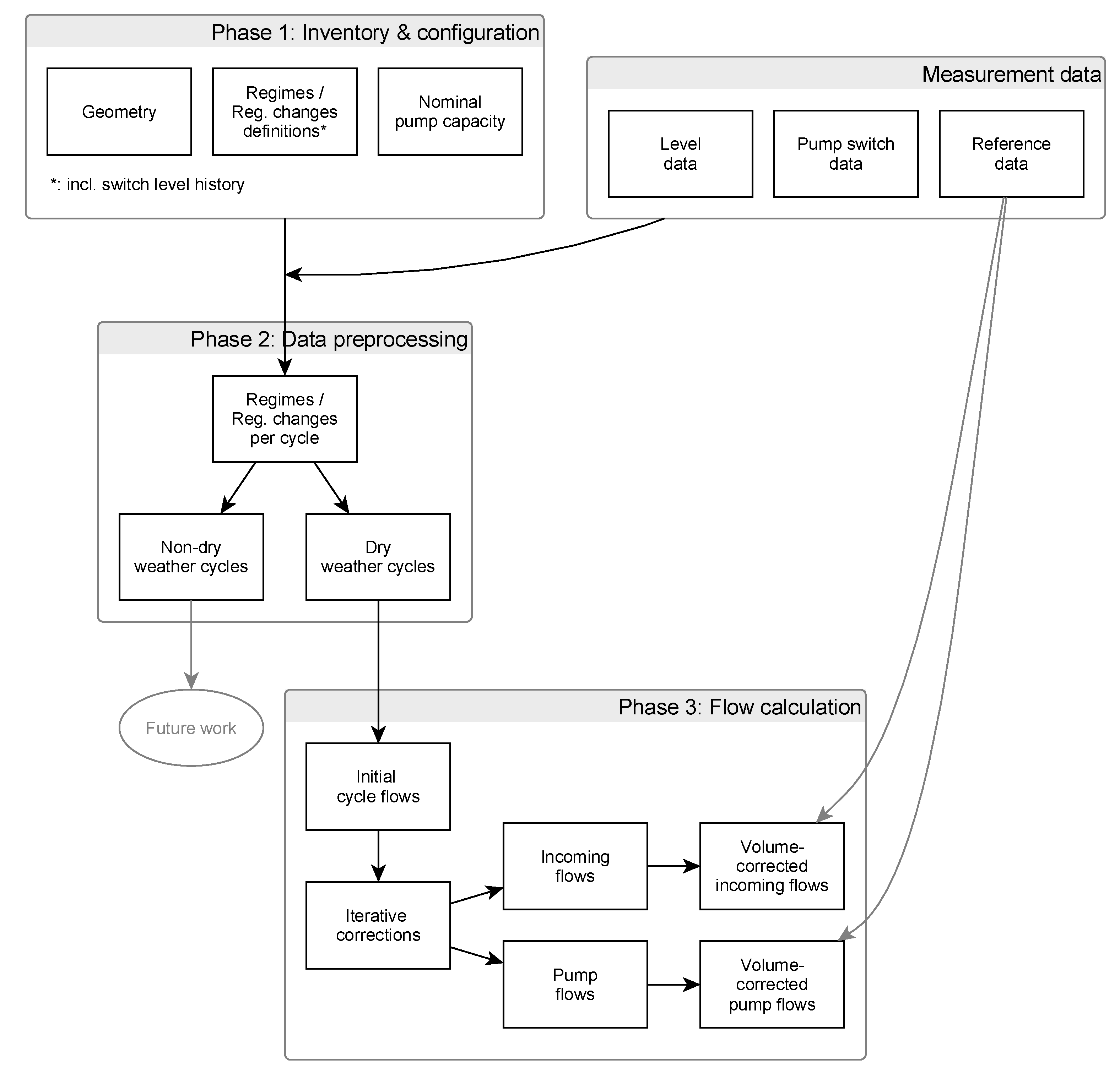
The methodology proposed in this paper consists of three phases, as shown in Figure 1: (1) an inventory of the configuration and the operational modes of the pumping station; (2) a data preprocessing phase; (3) an iterative calculation of average incoming and outgoing flows for all dry weather cycles. In the following paragraphs, the different phases are explained in more detail.
Throughout the methodology, the term “dry weather” should not be seen as a strictly meteorological condition but as a situation during which the water level in the pumping station is not exceeding the lowest switch-on level. Depending on the installed pump capacities, this can include periods of light-intensity rainfall runoff.
2.1. Inventory and Configuration Phase
For a pumping station containing Np pumps, a total of potential pump status combinations (SC) can be defined. These are all the theoretical combinations of the different pumps being idle or active. The total number of transitions from one status combination to another, further called pump status combination changes (SCC), equals . These SCs and SCCs can be grouped in operational regimes and regime changes: e.g., all SCs that contain a single active pump can be grouped into a regime “single pump use”; all SCs that contain two active pumps can be grouped into a regime “double pump use”, etc. Possible regime changes are then, e.g., the switch from “single pump use” to “double pump use” or vice versa. Appendix A gives an elaborated example of the operational regimes and regime changes for a typical “2 + 1” pump configuration (2 active pumps + 1 spare).
The inventory and configuration phase consists of identifying all actual operational regimes and regime changes for the considered pumping station and the related operational settings for switch-on and switch-off levels. Those associated with dry weather conditions are labelled as “dry weather regime change”. Additional information and an example are given in Appendix A. Based on available pump curves, the nominal pump capacity for each pump is estimated for the different regimes in which they can be active.
Another aspect of the inventory is the description of the geometry of the pumping well and the incoming pipes. Storage volumes should be described via tables of volume vs. level, rather than as a limited set of fixed volumes between predefined levels. This makes it possible to deal with multiple or time variable switch levels in the most flexible way during the data preprocessing and flow calculation phases (see further). For the pump well, such tables can be produced, e.g., using the most detailed information available (design or construction plans, 3D surveys via Lidar, hydrodynamic models, or other reliable sources). For the incoming pipe storage, volumes can be calculated based on their geometry (diameters, invert levels). Some hydrodynamic modelling packages contain built-in functionalities to generate such storage volume curves.
2.2. Data Preprocessing Phase
In this phase, the raw time series of pump switch-on/-off timestamps and level data are processed in combination with the regime and regime change details resulting from the above-described inventory and configuration phase.
The first purpose of the preprocessing is to identify errors in the raw pump data, i.e., sequences of switch-on and -off registrations that do not yield valid regimes or regime changes (e.g., one pump switch-on followed by a switch-on of the same pump). Such errors can occur when certain switch registrations were lost during the data collection or because manual switch-on/-off operations have taken place during maintenance interventions.
The second purpose of preprocessing is to analyse gaps in the data. Sometimes gaps are clearly too long to represent a real period during which no pump switching took place. They do not necessarily, however, lead to invalid regimes or regime changes because in theory the last and first registration before and after the gap may still yield a valid sequence. Most PLC (Programmable Logic Controller)-controlled pumping stations have a built-in maximum period during which one and the same pump may remain active (leading to regime changes Sx and Dx, as explained in Appendix A). This maximum time can be used to identify potential gaps in the raw data. Whenever data cannot be assigned a valid regime or regime change or when a gap has been identified, the data set has to be split up into independent subsets to prevent flow calculation errors in further steps of the methodology.
After correcting invalid and missing data, the remaining data subsets consist of a series of pump cycles. These are either filling cycles, which start with a switch-off and end with a switch-on, or emptying cycles, which start with a switch-on and end with a switch-off. Both types of cycle can also contain multiple intermediate timestamps where one pump is replacing another because of the exceedance of the maximum pump time (cfr. the Sx and Dx regime changes, as described in Appendix A). Pump cycles that start and end with a regime change that is labelled as a “dry weather regime change” are classified as “dry weather cycles”. As explained above, they can be divided further into “dry weather filling cycles” and “dry weather emptying cycles”.
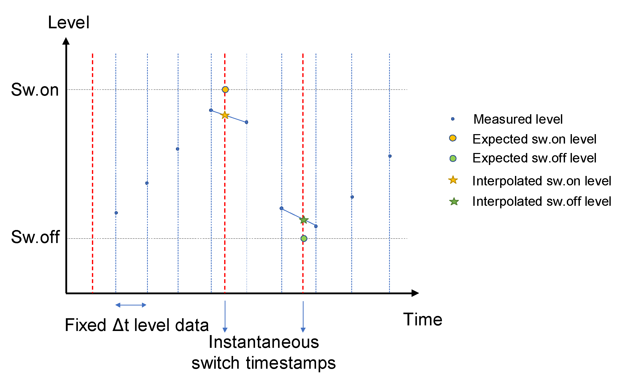
The concept of pump cycles is the key to the flow calculation phase. As will be explained hereafter, an initial cycle-based flow calculation can be performed purely on the basis of pump switch registration data. Water level data are only required in specific cases to improve this initial calculation. However, if level data are available, a useful additional data preprocessing step is the calculation of interpolated levels at the timestamps of switch-on and switch-off. These interpolated values provide a double check of the pre-assumed switch-on and switch-off levels (and the storage volumes corresponding to these levels). Similarly, they can be helpful to identify unknown changes in the level settings when their history is not logged. Appendix B describes how different interpolation methods can be used to avoid obvious errors in purely linear interpolation.
2.3. Flow Calculation Phase (Cycle Based)
At the end of the preprocessing phase, a list of dry weather filling and emptying cycles is available with their respective start and end times, cycle durations, and switch-on/-off levels. For all these cycles, the cycle-averaged incoming and outgoing flows can now be calculated.
In general, the continuity equation in a pumping station during dry weather flow (Equation (1)) can be formulated as
where
V (t): the instantaneous volume stored in the pumping station (m3);
Qin (t): the flow entering the pumping station (m3/s);
Qout (t): the flow pumped out from the pumping station (m3/s).
When applied over a full pumping cycle this yields
and
for, respectively, a filling cycle (Equation (2)) and an emptying cycle (Equation (3)),
where
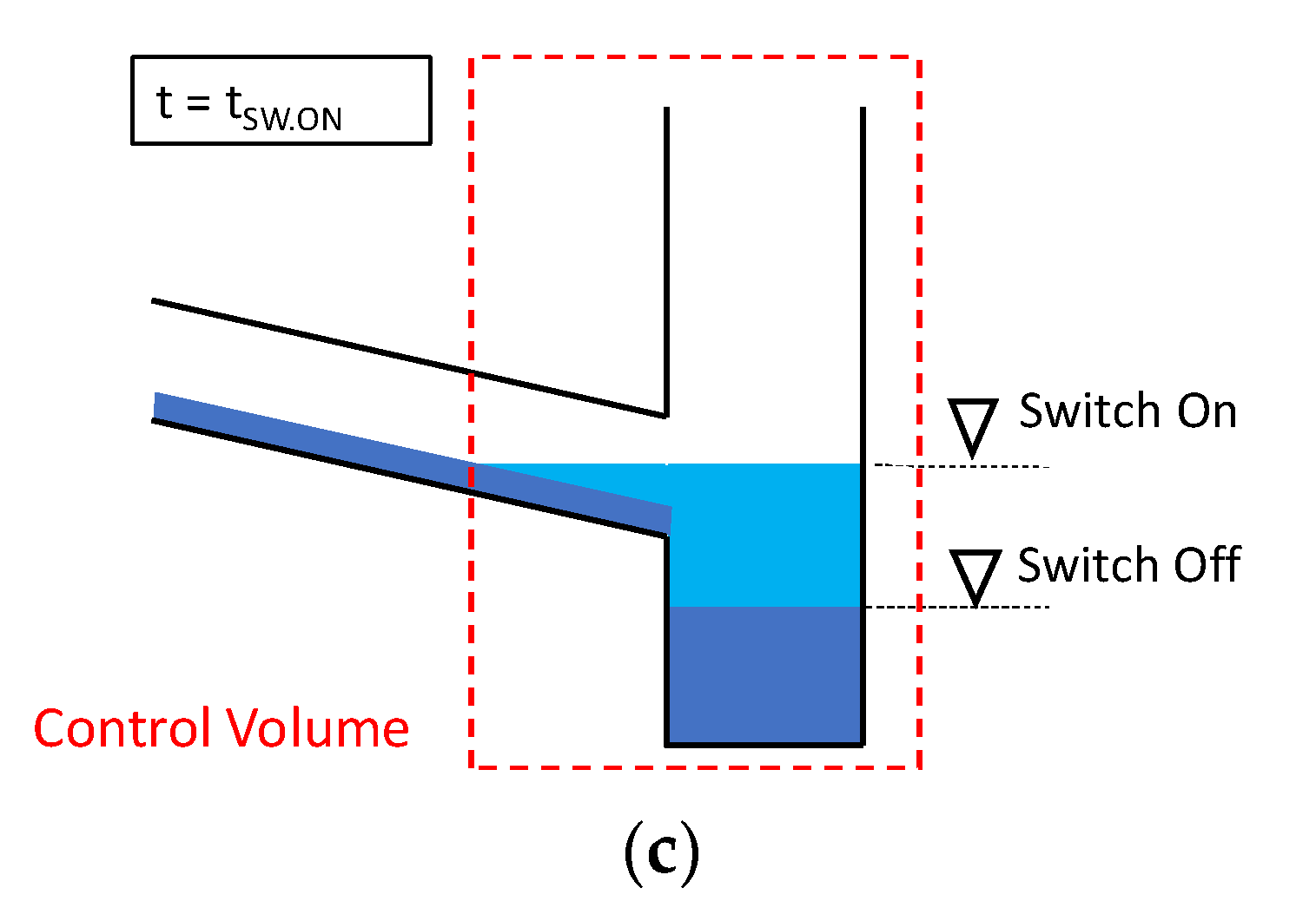
VDWF: the control volume between the dry weather switch-on and switch-off level (m3) (see Figure 2);
: the average incoming flow during the filling cycle (m3/s);
: the average incoming flow during the emptying cycle (m3/s);
: the average pumped flow during the emptying cycle (m3/s);
Δtfill: the duration of the filling cycle (s);
Δtempt: the duration of the emptying cycle (s).
This means that cycle-averaged incoming flows can be calculated for all dry weather filling cycles using only the instantaneous timestamp registration of the pump switching on and off and the dry weather control volume. Moreover, assuming that cycle-averaged dry weather flows will not vary significantly between two consecutive filling cycles, of the intermediate emptying cycle can be estimated from the preceding and following values of only (e.g., by linear interpolation). This, in turn, allows one to calculate the average pump flow during the intermediate emptying cycle from Equation (3).
In Equations (2) and (3), VDWF is assumed to be constant. However, in reality, settings of switch levels can change over time, meaning that during the processing of longer data sets, VDWF can vary throughout the data set. This has to be handled during the data preprocessing phase, resulting in a list of VDWF values per cycle.
Sometimes, a pump’s switch-on is not only defined by level but also by the maximum duration of the filling cycle. This can be the case, e.g., for wastewater treatment plants where a maximum idle time of the influent pumps is imposed to ensure the stability of the treatment process and/or to prevent sedimentation build-up in the incoming collector. In such cases, VDWF for the shortened cycles must be calculated by using the interpolated level at the moment of forced switch-on.
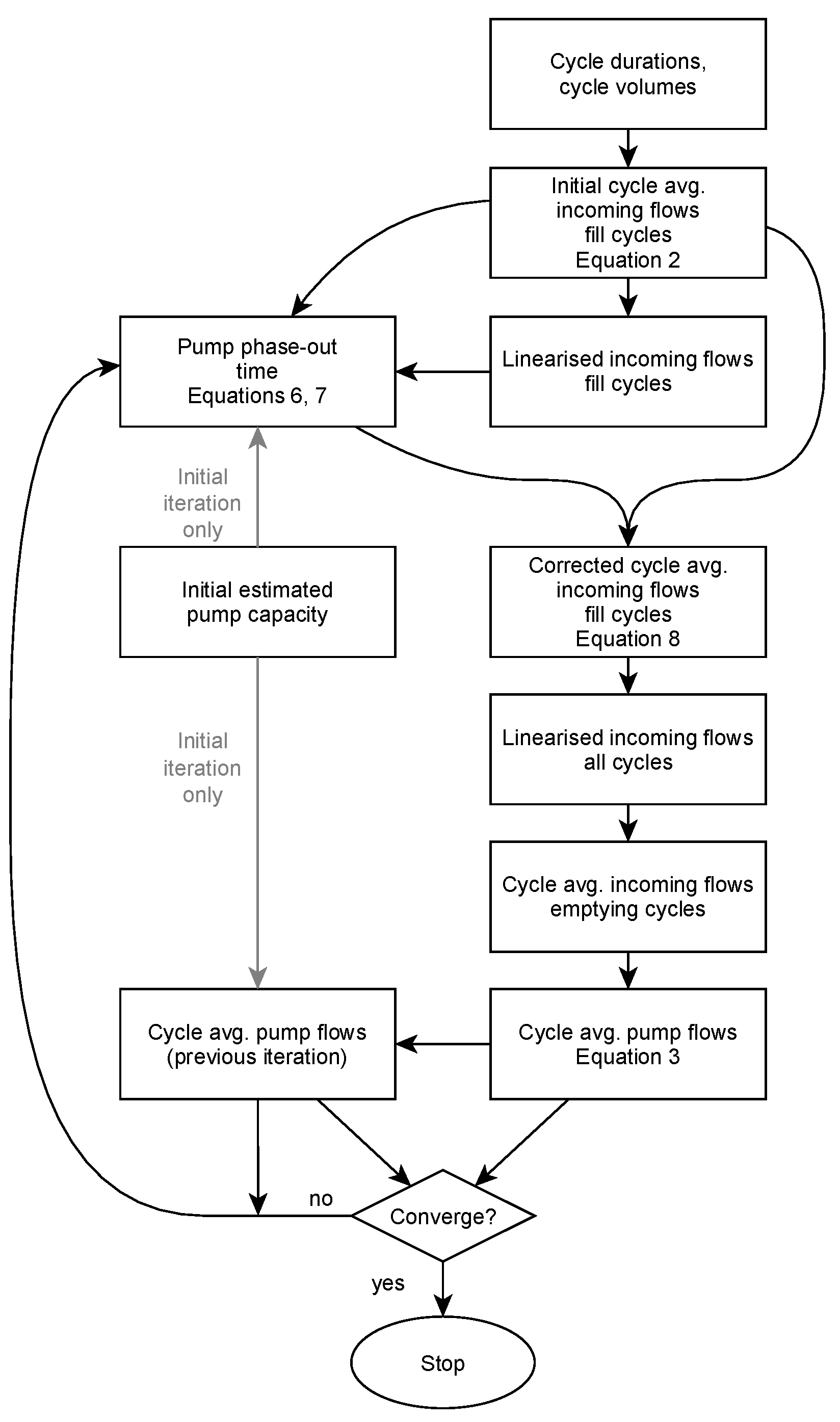
Because the above-described basic flow calculation is still prone to a number of uncertainties and assumptions, an iterative correction procedure is required to yield more accurate results. This is shown in Figure 3 and described in detail in the following paragraphs.
2.4. Linearising the Cycle-Averaged Flows
The incoming flows during filling cycles, as calculated from Equation (2), are average values over the duration of the cycles, whereas, in reality, flows are a continuous function of time. Assuming that dry weather flows will generally not show sudden variations over the relatively short duration of a pumping cycle, a linearisation of the average values is proposed to create a more continuous transition between successive cycles.
This is carried out by averaging gradients between successive filling cycles. During this process, it is important to preserve volumes per cycle, as these are the direct results from Equation (2) and hence should not be smoothened out. This linearisation procedure is illustrated in Figure 4: the cycle-averaged incoming flow Qin,2avg for cycle 2 is transformed into a time-dependent flow varying linearly between Qin,2,1 at time t2,1, the start of the cycle, and Qin,2,2 at time t2,2, the end of the cycle. The gradient of this linear variation during the cycle is found by averaging the gradients of the lines that connect the average flows of the successive filling cycles at their respective midpoints. After this linearisation of the filling flows, the flows during the emptying cycles are calculated as linearly varying flows by connecting the end and start values of the linearised flows of the surrounding filling cycles.
2.5. Correction for Phase-Out Time of Pump Flows
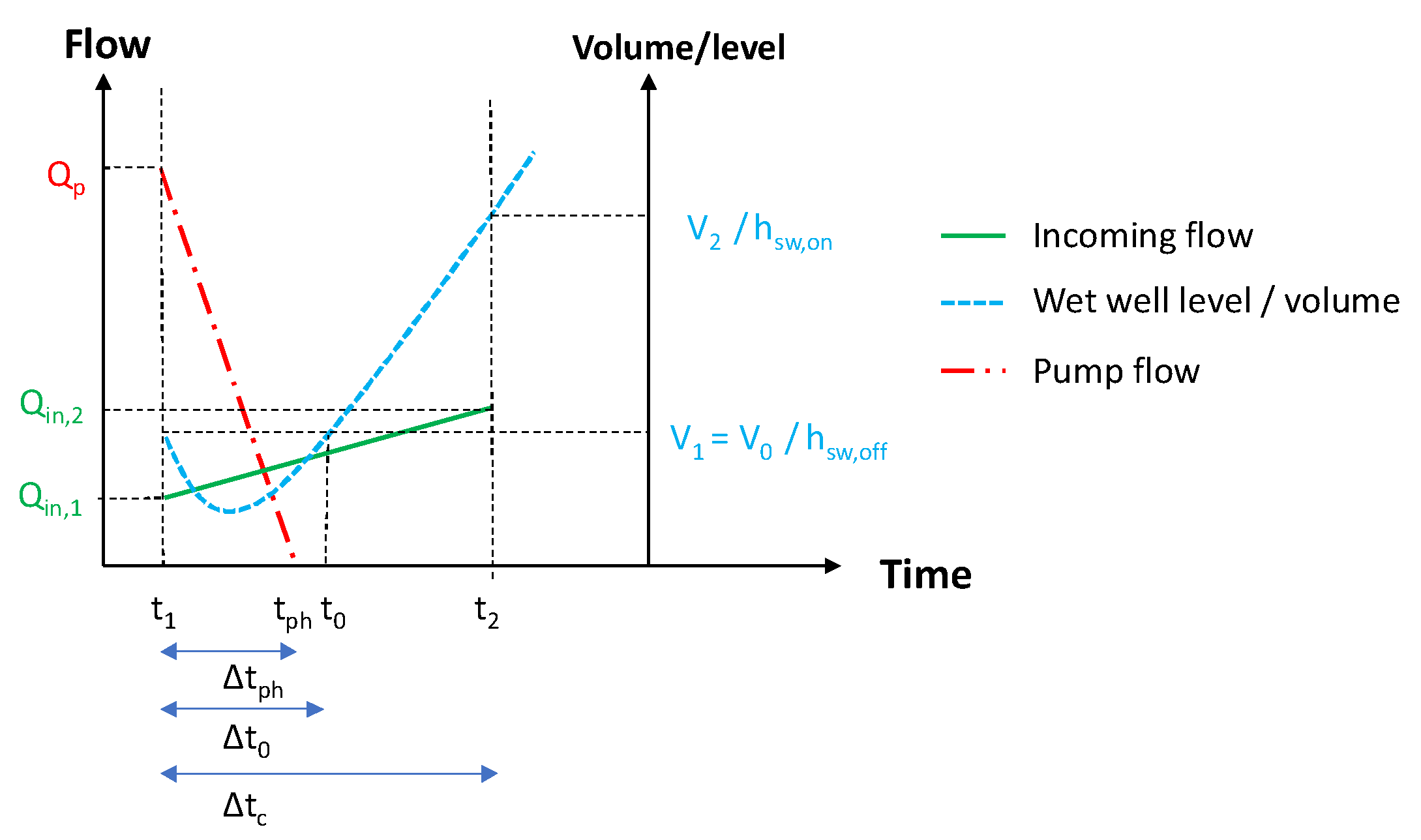
When pumps are switched off, as a result of inertia, they continue to pump some volume for a limited amount of time (the phase-out time Δtph). In some cases, this can cause the water level in the wet well to continue dropping down after the pump has switched off. A similar phenomenon occurs at the switch-on of pumps: because the pump has a delay time to reach its full capacity, the water level can initially continue to rise above the switch level. However, this delayed start does not affect cycle-based calculations and therefore will not be considered further here.
Because Δtph is not known, it must be derived from the observed time at which the level reaches the switch-off level again after the initial dropdown. This is further indicated as the zero-level recovery time, or Δt0 (see Figure 5). In many cases, it will not be possible to derive Δt0 from the available level records. Either the time during which the level drops down below the switch-off level can be shorter than the time interval of the available level data series, or the combination of the incoming flow and pump flow can be such that the water level does not initially drop down at all. In such cases, Δtph is set to 0.
Assuming (i) a linear decrease in the pump flow between of the past emptying cycle at switch-off time t1 and zero flow at the (still unknown) time tph (=t1 + Δtph) and (ii) a linear variation of the incoming flow between Qin,1, at switch-off time t1, and Qin,2, at switch-on time t2, with the cycle duration ∆tc = t2 − t1, Δt0 can be calculated as:
or
for, respectively, ∆t0 ≤ ∆tph (Equation (4)) and ∆t0 ≥ ∆tph (Equation (5)).
Both equations can now be rewritten to derive ∆tph from the observed ∆t0, which yields Equation (6) for ∆t0 ≤ ∆tph:
and Equation (7) for ∆t0 ≥ ∆tph:
By grouping all fill cycles according to which pump was active in the preceding emptying cycle, all individual cycle values of ∆tph can now be consolidated into a single median value per pump (p = 1…NP). The limitation of this procedure is the assumption that no more than 1 pump is active during dry weather emptying cycles.
Based on this value, Equation (2) can be modified to calculate a corrected value of for all fill cycles (yielding Equation (8)):
2.6. Further Iterative Calculation of Pump Flows and Incoming Flows
As shown in the detailed flowchart in Figure 3, the corrected average incoming flows of the different fill cycles, as obtained from Equation (8), can form the start of an iteration loop.
Using again the linearisation procedure on the corrected values of , corrected linearised incoming flows for the emptying cycles can now also be calculated (as shown in Figure 4), and from these, corrected values of and, using Equation (3), corrected values of for each pump are obtained.
Corrected values of can now be compared to the previously calculated value, which, in the first iteration, is equal to the initially estimated nominal pump capacities. If the difference for each pump is within a preset tolerance, no further iteration is required. If not, the new values of are used as input for a new calculation of the pumps’ phase-out times, which will then again be used in Equation (8) to calculate new corrected incoming flows, until convergence for is achieved.
Even if no pump phase-out times can be calculated, and hence no correction needs to be applied to the fill cycles’ incoming flows, at least one iteration will generally be necessary to validate the initial assumption of the pumps’ nominal capacities.
3. Results
In order to implement the methodology described above, a dedicated tool was built in Matlab [38].
Four pumping stations (PS Vuntlaan, PS Wijgmaalsesteenweg, PS Zuidstraat—all three in drainage area Leuven—and PS Wauberg—in drainage area Peer) were chosen as pilot sites for testing the methodology. A short overview of their characteristics and the connected catchments is given in Appendix C, together with an overview of the necessary input data and an example of the result of data preprocessing.
3.1. Results of the Flow Calculation Phase
With the cycle-based approach, incoming flows and pumped flows are calculated for every dry weather cycle. Next, these flows are postprocessed and presented in detailed graphs per day and in overview graphs with daily values. It is important to take into account that for days containing both dry weather and non-dry weather cycles, daily volumes will be an underestimation of the real values, as no flows are being calculated for the non-dry weather cycles.
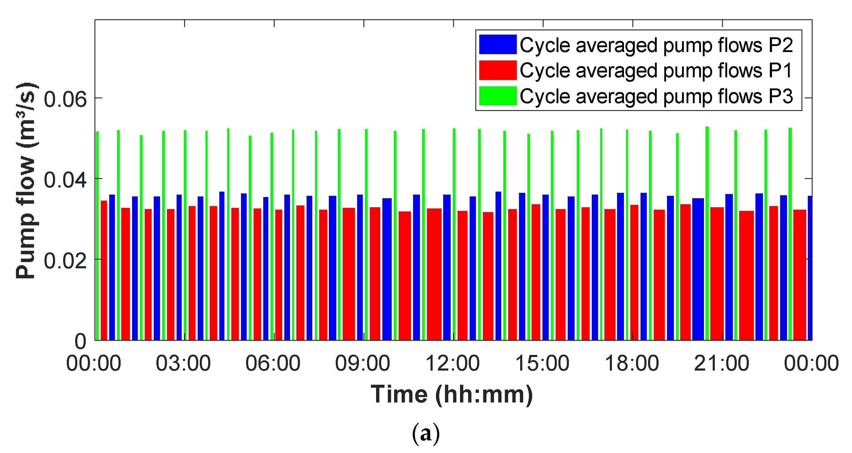
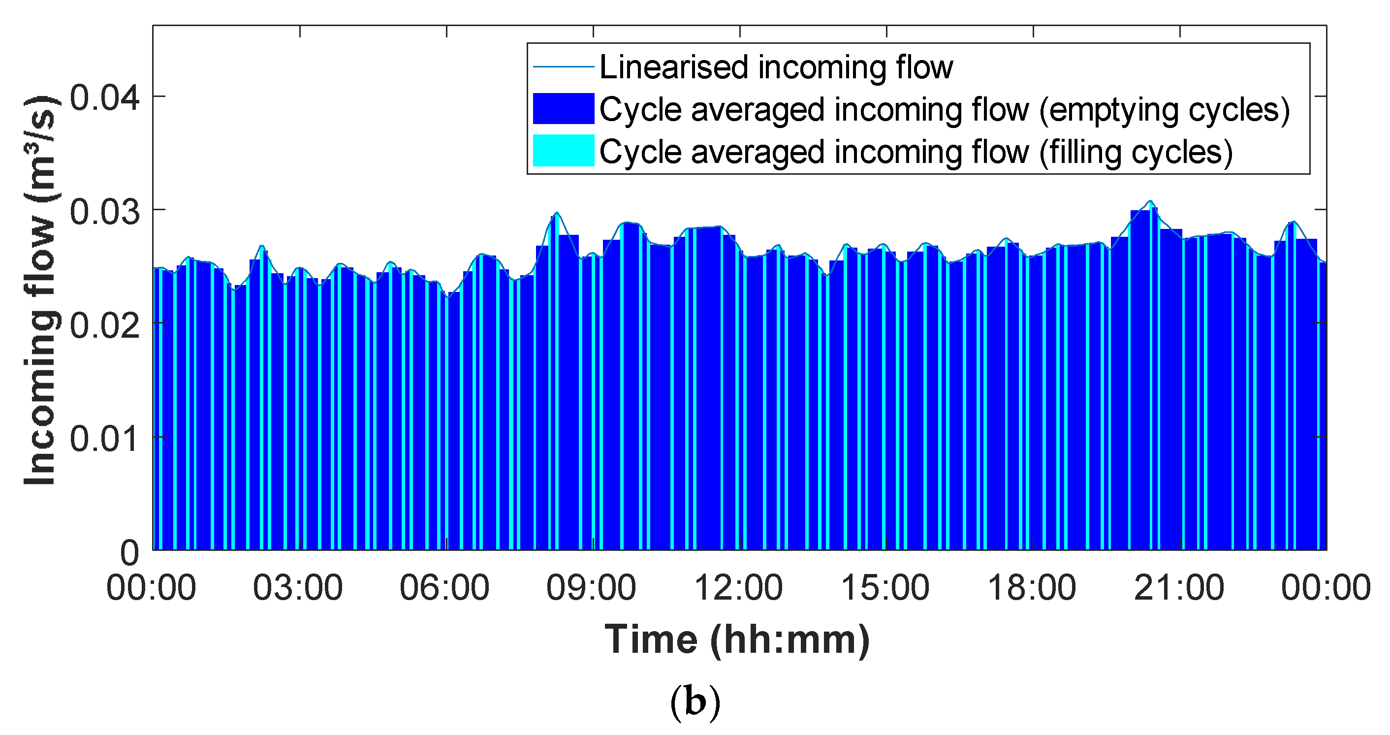
Figure 6, Figure 7 and Figure 8 all show the detailed results of the calculated incoming flows and pumped flows during a dry day.
In Figure 6, the two pumps have a very similar calculated flow, which is very close to the assumed nominal capacity (31 L/s). In Figure 7, although the results are about twice as high as the initially assumed nominal capacities (18 L/s for pump1 (P1) and pump2 (P2), and 27 L/s for pump3 (P3)), the ratio between the different pump capacities is preserved. This proves that the methodology is capable of handling such cases without affecting the continuity of the resulting incoming flow curve. The most likely reason for the large deviation of the calculated pump capacities is the overestimation of the control volume VDWF (see further, Section 3.2).
In Figure 8 on the other hand, there is a clear discrepancy between the calculated pump flows and the calculated incoming flows. The pump flows—as expected from the available pump curves—are very similar for both pumps. The incoming flows, however, show significantly different values for the different cycles, depending on which pump was active. In this case, after an investigation on-site, there appeared to be a problem with the wiring of a provisional datalogger. This resulted in one of the pumps failing to log its switches, although it was operating normally. Because of the regular alternation of the three pumps, this did not result in the erroneous identification of regimes and regime changes. However, the calculated cycle duration for the cycles preceding the non-logged ones was not reflecting the real cycle duration and, therefore, yielded lower calculated average cycle flows. Note that in this case, the calculated flows for P2 and P3 are only around two-thirds of the expected value (69 L/s). Additional measurements have to clarify whether this is due to an underestimation of the control volume or if the pumps are not reaching their envisaged capacity.
3.2. Estimation of the Uncertainty of the Results
As can be seen from Equations (2) and (3), the calculated flows are directly proportional to the assumed VDWF, and the relative error on the calculated flows δQ equals the sum of the relative errors of the control volume and the cycle duration (δVDWF + δ (Δtc)). From these two parameters, the control volume is the one with the highest uncertainty. Even if detailed information to calculate this volume is available, it remains very difficult to account for space taken up by objects such as pump bodies, lifting chains, rising mains and valves, ladders, and benchings. Therefore relative errors of >10% on VDWF are not unusual. If the control volume extends well into the incoming pipes, this error may be even higher, as explained in Appendix D.
The accuracy of the cycle durations, on the other hand, based on specifications of the SCADA system employed for data communication and logging, is of the order of 1–2 s. With (dry weather) cycle durations rarely being lower than 5 min, the relative error is thus generally well below 1% and hence can be considered negligible in comparison with δVDWF.
The (high) uncertainty of VDWF and hence of the calculated flows can be reduced if independent flow measurements are available. Because the incoming flows and the pump flows are linked by the continuity equation, it takes only one reference flow, either the incoming flow or the pump flows, to correct both calculations.
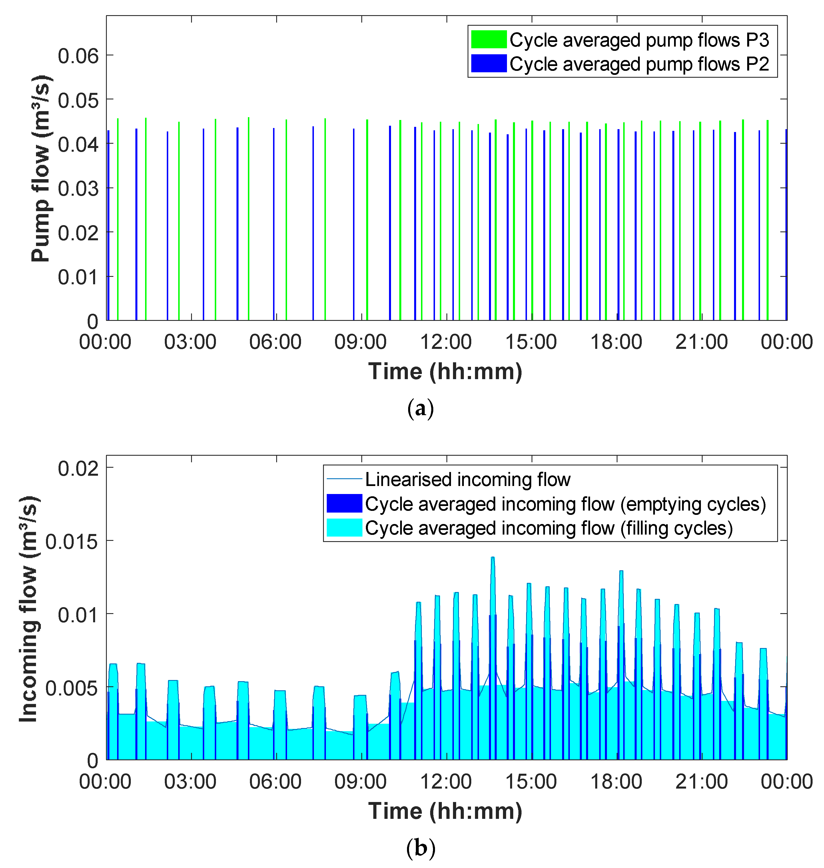
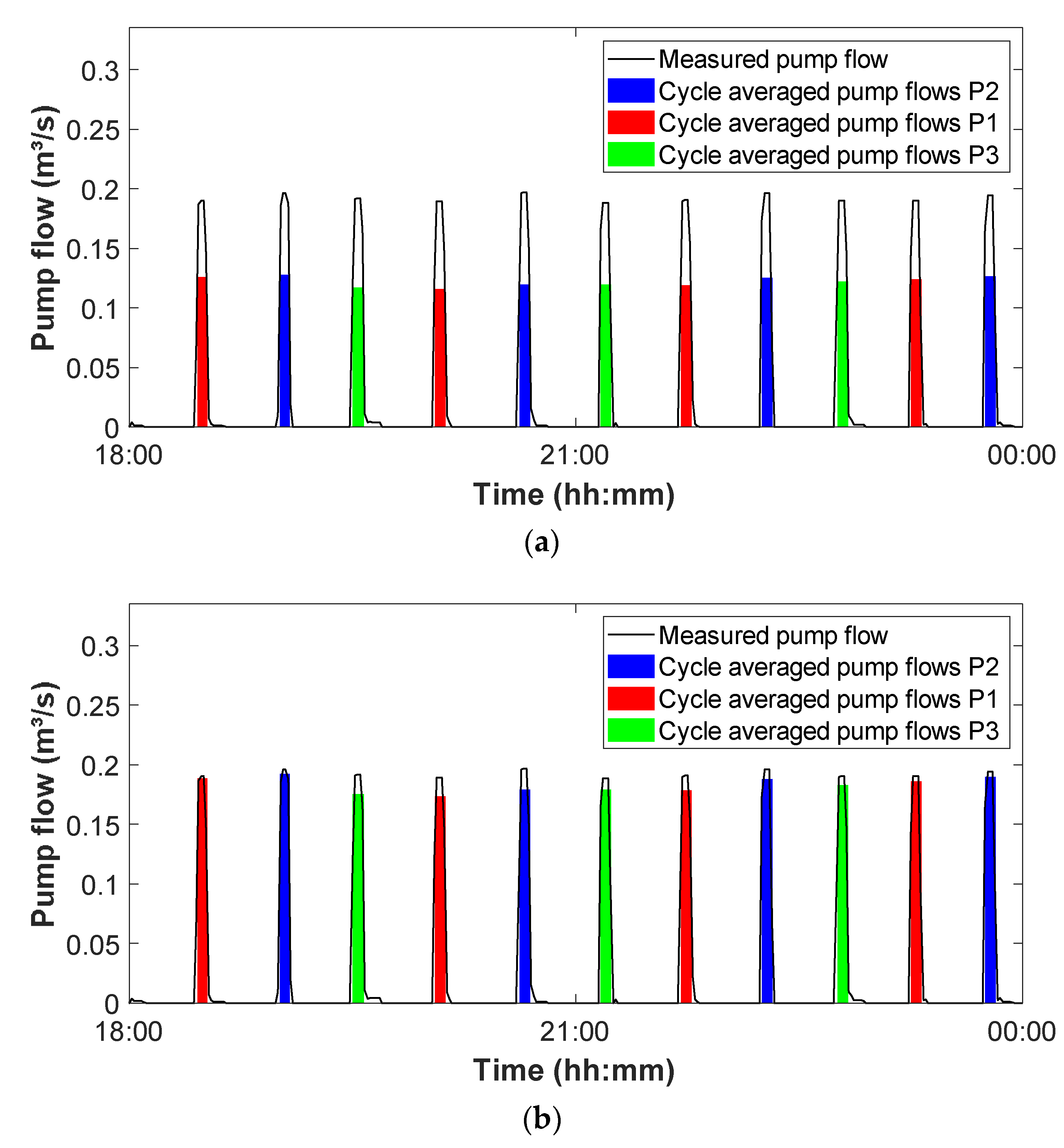
When reference flows are available, a correction factor Kvol can be determined from the comparison between reference and calculated flows, e.g., based on daily volumes or averages. Because of the linear relationship, as expressed in Equations (2) and (3), the calculated flows simply need to be multiplied by this correction factor. This is illustrated in Figure 9, where reference pump flows are available from electromagnetic flow meters at the rising mains. The remaining deviations between the calculated and measured pump flows per emptying cycle after correction are due to (i) the differences between the fixed time interval of the measurements (1 min) and the instantaneous registration of the switch times (resolution 1 sec) and (ii) the variability of the pumped flows over the duration of the cycle as a result of the pumps being variable-frequency-driven.
When VDWF varies over time due to varying switch-on/-off levels or forced switch-on, multiple correction factors have to be determined for different periods. Moreover, when the flow dependency of the in-pipe control volume would have a significant impact on the calculated flows, a simple linear correction may not be sufficient to bring the calculated flows in accordance with reference flows. This is explained in more detail in Appendix D. More investigation is needed to assess what accuracy can be obtained in such cases.
Even if no reference flows are available (which may often be the case), upper and lower limits of incoming flows and pump flows can generally be estimated based on available pump curves and expert knowledge of the sewer system and the catchment connected to it. This may then already be a useful first step to eliminate large errors in the estimation of the storage geometry.
3.3. Identifying the Presence of Inflow and Infiltration
The objective of this paper is primarily to present a methodology for calculating flows at pumping stations and not to propose algorithms for quantifying I&I contributions to these calculated flows. Nevertheless, some example results show that the high temporal resolution of the calculated flows can contribute to facilitating the quantification of I&I.
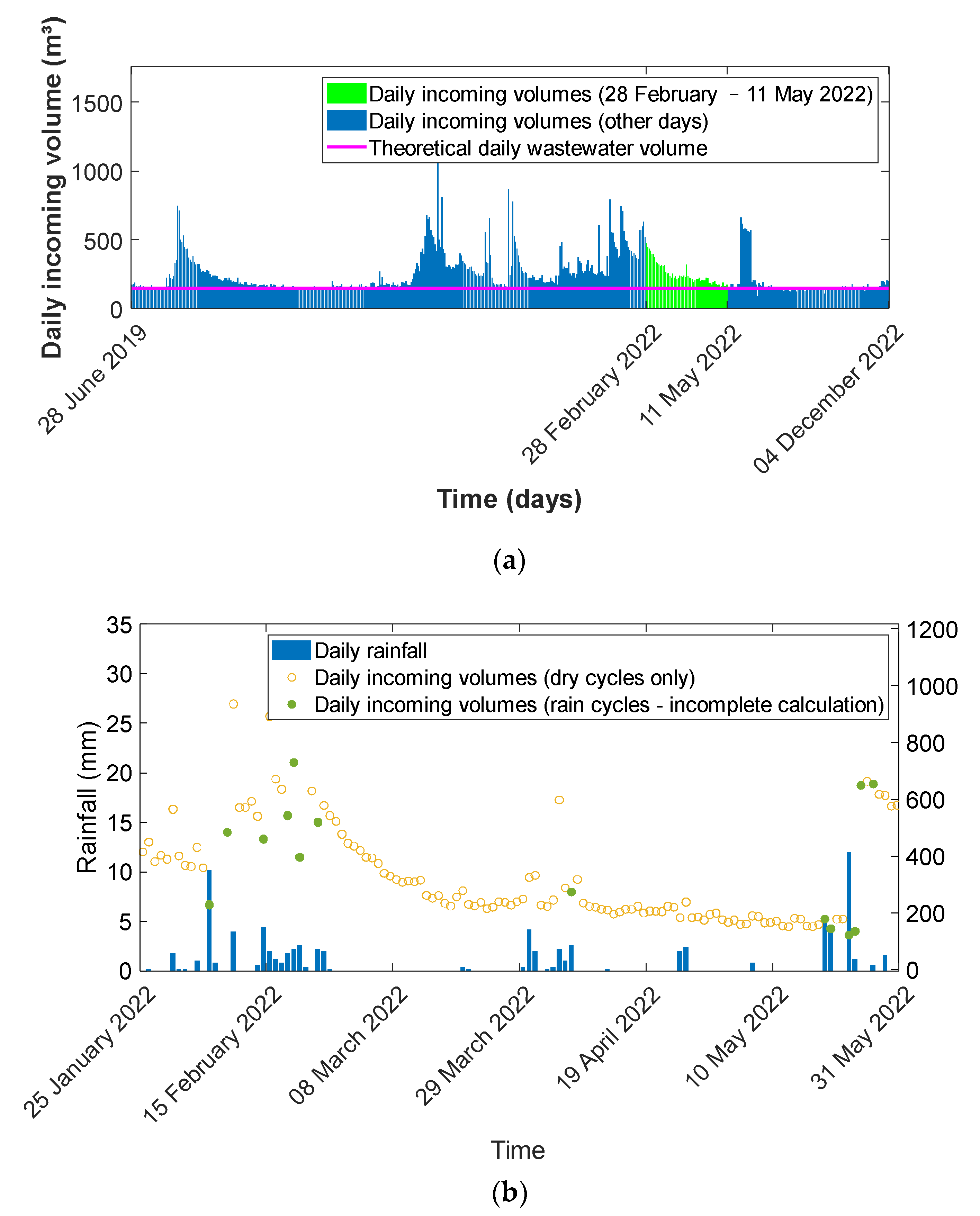
Figure 10a shows the overview of daily volumes for these days that only contain dry weather cycles. The main reason for omitting the other days is that incoming flows (and hence the daily volume) can only be calculated for dry weather cycles. The severity of the underestimation for each day depends on the number and duration of non-dry weather cycles for that day. This variation of underestimations would complicate the interpretation of the graph if all days were shown. This is illustrated in Figure 10b for a selected period where the daily rainfall is shown against the calculated daily volumes.
The typical exponential decay of infiltration flows during long dry-weather periods can be detected even with only the results of the dry weather days, as can be seen in Figure 10a. A more detailed analysis of the occurrence of I&I can be made by selecting the relevant days from such periods and comparing the calculated daily flow patterns.
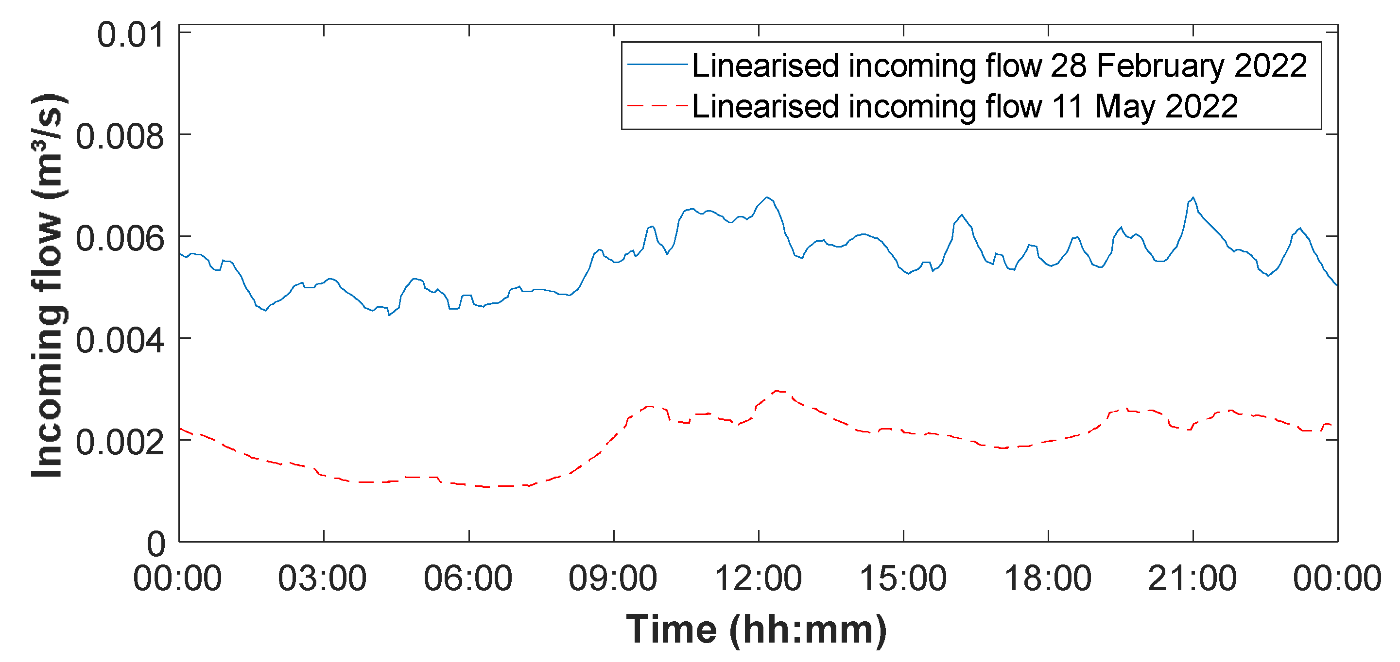
Figure 11 shows the detailed calculated incoming flows for the first and last day of the selected period between 28 February 2022 and 11 May 2022, during which there were only a few days with (insignificant) rain. As can be seen, the high initial infiltration flow offsets the diurnal wastewater profile. Although the two profiles are very similar, the one for 28 February shows less variability. When both patterns are normalised to their respective average value, the one with the higher infiltration flow thus becomes more flattened.
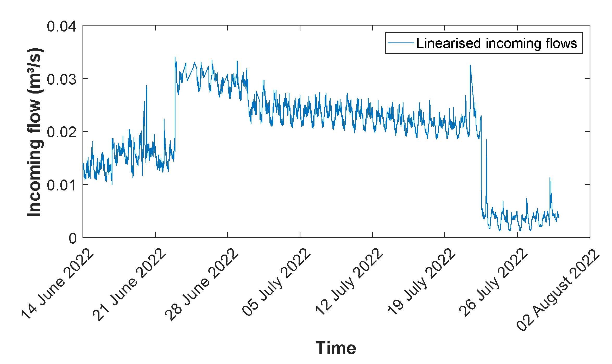
A typical example of high I&I originating from the pumped groundwater drainage of a construction site is shown in Figure 12. Especially when such I&I contributions coincide with periods of rainfall-dependent infiltration, they can impede the proper calibration of hydrologic models when only daily volumes are available.
Note that the flows in Figure 12 are still unvalidated. As shown earlier in Figure 7, the calculated pump flows at this location are about twice as high as the assumed nominal capacities (more precise values may be derived from additional reference measurements). The same correction needs to be applied to the calculated incoming flows. Nevertheless, the pattern showing the impact of the pumped groundwater drainage will remain unaffected by this correction.
4. Discussion
In the above results section, it has been demonstrated that for every pumping station where the necessary data and measurements are available, incoming dry weather flows can be calculated at high temporal resolution. The prerequisites for the methodology to be applicable are (i) the availability of instantaneous pump operation registrations; (ii) preferably, but not mandatorily, the availability of level measurements with sufficient temporal resolution (typically 1 min); (iii) the availability of geometry data for both the pump well and the incoming pipes; (iv) the availability of information about operational regimes and switch levels; (v) under normal dry weather conditions, pumps should not be permanently active; and (vi) the availability of some reference flow measurements for validation purposes (minimum required temporal resolution: daily volumes). These can be either incoming flows or pumped flows and do not need to cover the whole timespan of the analysed data.
The temporal resolution of the results is the pumps’ switch frequency. On average, in dry weather conditions, this frequency can range from once every 1–2 h during low flows to once every 10 min during higher flows. Because the switch frequency is automatically adapted to the magnitude of the incoming flow, this is an intrinsic guarantee that the temporal resolution of the calculated flow is always in line with the expected variation in the flow pattern. Only in very specific circumstances, the switch frequency during dry weather will be too low to identify patterns in the flow. This can be the case, e.g., when a very small amount of PE (population equivalent) is connected, or when the installed pump capacity is much larger than the theoretical wastewater flow, expected on the basis of the connected number of PE. For such cases, a future extension of the methodology based on fixed timesteps (see further) will be necessary to yield useful results.
With the current state of the methodology (cycle-based calculation) it is possible to generate incoming flows, not only for dry periods but equally for periods with light rain where the runoff flows do not exceed the pump capacity (usually, three to six times the designed wastewater flow). This is an added value in comparison with hydrograph decomposition methods based on daily volumes [31]. Even for days with intense rain in the last hours of the day, incoming dry weather flows will still be reliably calculated for the larger part of the day. Daily volume-based methods, on the contrary, will classify such days as rainy days because of the important contribution of rainfall runoff.
The results also show that non-rainfall-related contributions (e.g., from pumped groundwater drainage at construction sites) can be easily distinguished from the other more slowly varying I&I contributions. The main condition for this is that the pumping station is close enough to the location of such inflows and that the flows are significantly higher than the other dry weather components.
The methodology is equally applicable to systems that are predominantly affected by exfiltration rather than by infiltration. The main difference will be in the shape of the resulting dry weather flow hydrographs (more peaked, and in extreme cases potentially containing periods with zero flows). In general, though, it will be very hard to make a quantitative statement on the mutual ratio of exfiltration and infiltration. In specific cases, a comparison between the results from neighbouring locations might give an indication, but most often, an additional tracing experiment will be required.
The accuracy of the calculated flows depends largely on the estimation of the control volume, compared to which the accuracy of the cycle duration is negligible. When the control volume is not or only marginally extending into the incoming pipes, the relationship between the calculated incoming flows, the calculated pumped flows, and the control volume is linear. This means that, when independent reference measurements are available, the calculated flows can be corrected by applying a simple linear correction factor. Such correction brings the accuracy of the calculated flows to the same level as the accuracy of the reference (direct) flow measurement. This remains valid even if the reference measurements are only available for a limited period of time. The only condition for a single correction factor to be applicable is that switch levels do not vary over the period of flow calculation.
The presented results are from a limited set of pumping stations that were temporarily equipped with a datalogger to capture the required pump switch and water level data. However, during the past three years, more than 1800 pumping stations, managed by Aquafin in Flanders (Belgium), have been equipped with a uniform SCADA system that collects these same and other data. This means that there are sufficient input data available to potentially produce detailed local flow profiles for all these locations by applying the methodology proposed here. In comparison with the effort required to install and maintain a similar number of permanent direct flow measurements, this novel approach makes it possible and affordable to aim at a systematic analysis, resulting in a better understanding and management of I&I flows in the urban drainage systems throughout Flanders, Belgium.
Finally, it must be stressed that the methodology does not only produce incoming flows but also pumped flows for each individual pump. These results have the same temporal resolution and accuracy as the incoming flows and have various additional benefits. On one hand, they will be useful for understanding the hydraulic behaviour of urban drainage systems and for improving hydrodynamic models as an operational tool (e.g., digital twins). On the other hand, they will also be extremely valuable for optimising asset maintenance schemes. Given the constant accuracy at which pump flows are calculated over longer periods of time, these long-term trending results will help to identify decreasing pump performance at an early stage and optimise complex pump control rules.
The current methodology is limited to cycle-based flow calculations. Especially for pumping stations with more complex configurations, this puts a limitation on the degree of accuracy that can be achieved. The envisaged solution for many of these special cases lies in a fixed timestep approach as a fourth phase, following the current cycle-based calculations. Such an approach, where continuity equations are performed at every fixed timestep within the different cycles, will require further iteration of already existing steps in the calculation. More important, however, is that it will mandatorily require level measurements with a sufficiently high measurement interval (as opposed to the cycle-based approach, where level measurements have an added value but are not strictly necessary). Other improvements will focus on cases where there is significant interaction between the pumping well and the incoming pipes, which will require flow-dependent volume corrections rather than a fixed correction factor.
The following is a non-exhaustive list of cases that will benefit from the time-step-based approach
- Pumping stations that have at least one pump permanently active during periods of minimum dry weather flow. This means that in such cases, there are no filling cycles without active pumps, for which the incoming flow is only a function of the control volume and the cycle duration.
- Pumping stations with only one set of switch levels that make it harder to distinguish between dry weather and non-dry weather cycles, especially for periods of light rain.
- Pumping stations with extremely low switch frequencies, where the low number of cycles per day does not allow the reliable linearisation of the calculated average cycle flows.
5. Conclusions
In this paper, a methodology is presented to derive sewer (dry weather) flow time series at a high temporal resolution from operational (SCADA) measurements at pumping stations. Such flow time series, in combination with rainfall time series, can contribute to a better understanding of the spatial and temporal distributions of inflow and infiltration (I&I) flows in large urban drainage systems. The application of the methodology to four test cases shows plausible results, which can easily be validated using short-term reference flow measurements. Besides the envisaged time series of incoming flows, the methodology also generates time series of pumped flows, which can be used to optimise preventive maintenance schemes for the pumps.
Author Contributions
Conceptualisation, methodology and original draft preparation: J.V.A.; visualisation, review and editing: S.K.; review and editing: R.D. All authors have read and agreed to the published version of the manuscript.
Funding
This research received no external funding.
Institutional Review Board Statement
Not applicable.
Informed Consent Statement
Not applicable.
Data Availability Statement
Not applicable.
Conflicts of Interest
The authors declare no conflict of interest.
Appendix A
The vast majority of pumping stations have a standardised configuration such as: “1 + 1” (two pumps, of which one is spare), “2 + 1” (three pumps, of which one is spare and two can work simultaneously), etc.
This appendix describes an example of the configuration for a “2 + 1” pumping station with three pumps of equal nominal capacity, which makes them all interchangeable in all regimes.
Number of pumps NP = 3;
Number of theoretical status combinations NSC = 8;
Number of theoretical status combination changes NSCC = 64.
Valid operational regimes for this configuration are:
- “zero” (no pumps working);
- “single” (1 pump working);
- “double” (2 pumps working in parallel).
Table A1 describes the theoretical status combinations (pump status 0 = idle; 1 = active) and the according operational regimes:

Table A1.
Status combinations and regimes for a 2 + 1 configuration.
| Status Comb n° | Pump1 | Pump2 | Pump3 | Regime |
|---|---|---|---|---|
| 1 | 0 | 0 | 0 | Zero |
| 2 | 0 | 0 | 1 | Single |
| 3 | 0 | 1 | 0 | Single |
| 4 | 0 | 1 | 1 | Double |
| 5 | 1 | 0 | 0 | Single |
| 6 | 1 | 0 | 1 | Double |
| 7 | 1 | 1 | 0 | Double |
| 8 | 1 | 1 | 1 | - |
In this case, status combination 8 is not a valid combination because there is no operational regime involving the three pumps working simultaneously.
Valid regime changes are:
- “single on” (S1) (transition from “zero” to “single” regime);
- “single off” (S0) (transition from “single” to “zero” regime);
- “double on” (D1) (transition from “single” to “double” regime);
- “double off” (D0) (transition from “double” to “single” regime);
- “single change” (Sx) (transition between “single” regimes with different status combinations);
- “double change” (Dx) (transition between “double” regimes with different status combinations).
The regime changes S0, S1, D0, and D1 all have an operational switch-on/-off level; Sx and Dx occur when one of the pumps has been permanently active for longer than a predefined maximum time, and hence can occur at any level. Strictly speaking, they consist of two other consecutive regime changes (e.g., Sx is a combination of S0 and S1), which occur in a predefined short time span (e.g., 0 to 5 sec). This grouping of quasi-simultaneous changes must be handled in the preprocessing phase of the data.
Table A2 summarises the relationship between the theoretical status combination changes and the regime changes. From these, only S0 and S1 are tagged as “dry weather regime change”, as the single pump capacity is assumed to be large enough to handle all expected dry weather flows. As a result of this, switch-on and -off levels for D0 and D1 are not expected to be reached during dry weather circumstances.
Table A2.
Status combination changes and regime changes for a 2 + 1 configuration.
| To Stat Comb | 1 | 2 | 3 | 4 | 5 | 6 | 7 | 8 | |
|---|---|---|---|---|---|---|---|---|---|
| From Stat Comb | |||||||||
| 1 | - | S1 | S1 | - | S1 | - | - | - | |
| 2 | S0 | - | Sx | D1 | Sx | D1 | - | - | |
| 3 | S0 | Sx | - | D1 | Sx | - | D1 | - | |
| 4 | - | D0 | D0 | - | - | Dx | Dx | - | |
| 5 | S0 | Sx | Sx | - | - | D1 | D1 | - | |
| 6 | - | D0 | - | Dx | D0 | - | Dx | ||
| 7 | - | - | D0 | Dx | D0 | Dx | - | - | |
| 8 | - | - | - | - | - | - | - | - |
In the case of more complex pump configurations where not all pumps are hydraulically interchangeable, different “single use” regimes could exist (as a result of different pump capacities). The potential transition from one “single use” regime to another should then not be considered as a change in the sense of the “single pump change” Sx, as described above. Similarly, in such cases, multiple “double pump use regimes” can be defined, as not all pumps with different nominal capacities can work in parallel in all combinations.
Appendix B
Different interpolation and extrapolation methods can be used to estimate the level value at the time of switch-on/-off (theoretically, this should be equal to the set switch levels).
The most straightforward method is a linear interpolation between the recorded level values immediately before and after the switch time. The only condition for this method to be applicable is the existence of at least one preceding/succeeding level record within the duration of the pump cycles whose start and end are defined by the switch. As can be seen from Figure A1, this method will, in principle, always underestimate the real switch-on levels and overestimate the real switch-off level. So, the real values could be estimated from the minimum/maximum value of a large number of interpolated values. In reality, however, short delays in the acceleration and termination of the pumps can cause the water level to temporarily exceed the switch levels. This makes the estimation on the basis of the minimum/maximum of linear interpolations less reliable. In practice, this method is only recommended if none of the following described alternative methods are possible, or in the case of pump changes that are due to the exceedance of a maximum pump time. In this latter case, the water level is assumed to be on a continuous part of the level curve. This makes the use of linear interpolation more justifiable.
Figure A1.
Estimation of switch levels by linear interpolation.

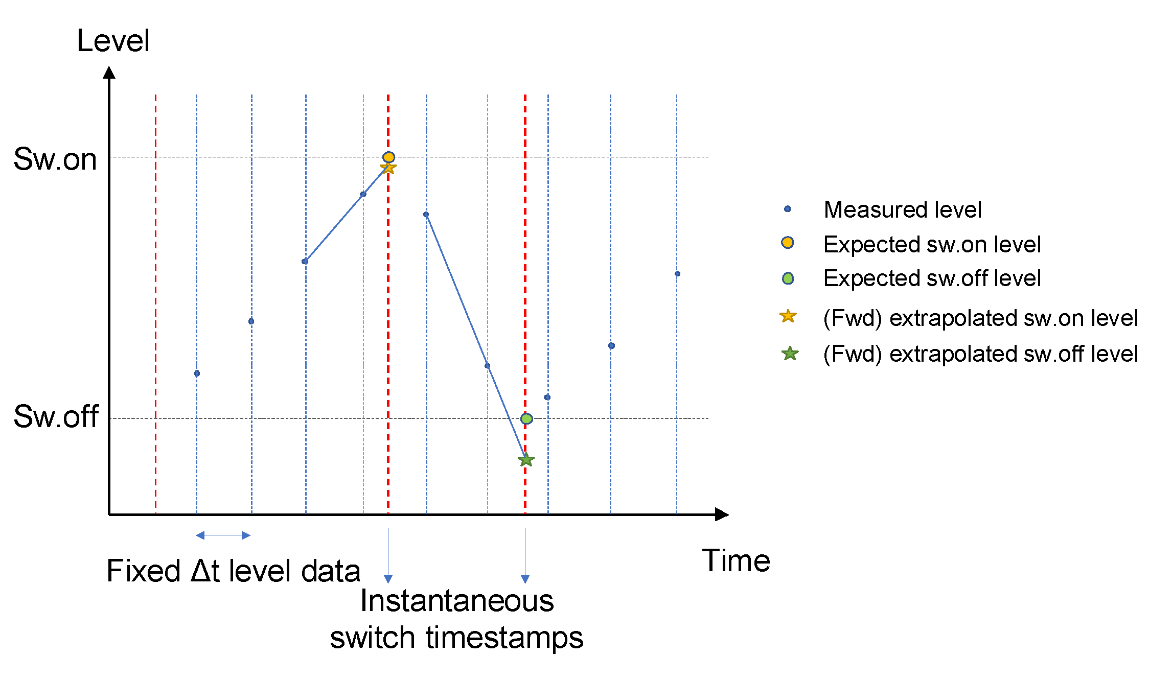
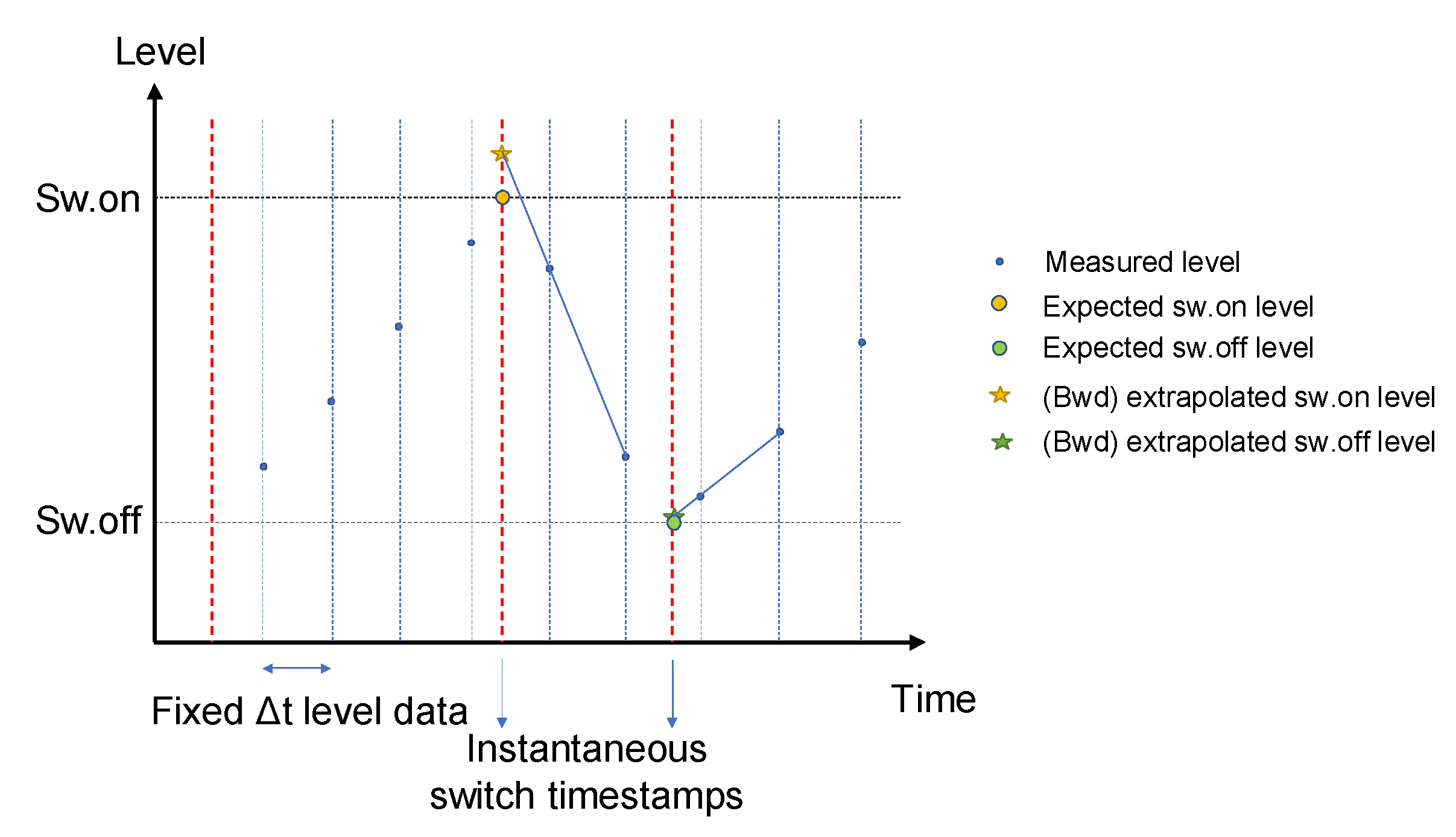
An alternative method to estimate the real switch level is to use linear extrapolation from two preceding or succeeding level records (respectively, forward and backward extrapolation). As for the linear interpolation method, this requires that at least two records exist within the duration of the preceding or succeeding pump cycle. Examples of both methods are given in Figure A2 and Figure A3.
Figure A2.
Estimation of switch levels by forward extrapolation.

Figure A3.
Estimation of switch levels by backward extrapolation.

With the extrapolation method, the calculated switch levels can be both an under- or overestimation of the real level. Therefore, it will be most appropriate to use the median value of a large number of cycles to estimate the real value. If there are no indications of level data below the switch-on or above the switch-off (as a result of delays in pump acceleration or termination), calculated values of the switch-on level should not be lower than the first recorded level of the next emptying cycle. Similarly, calculated values of the switch-off level should not be higher than the first recorded level of the next filling cycle. Such values should not be retained for the calculation of the median value.
Finally, a fourth possible method is the combination of forward and backward extrapolation. Consider a potential value of hsw situated between hsw,forw (i.e., the switch level calculated by forward extrapolation) and hsw,backw (i.e., the switch level calculated by backward extrapolation). For every such value, one can calculate the gradients of the level curves between hprec and hsw, on one hand (Sprec), and between hsw and hsucc, on the other hand (Ssucc). In this, hprec represents the last level record before the switch and hsucc is the first level record after the switch. These gradients can then be compared with the gradients of the level curves that are used for the forward and backward extrapolation (Sforw and Sbackw). The optimal value of hsw can be defined as the value that yields the minimum value of δS (the average relative difference with the extrapolation gradients) (Equation (A1)).
Appendix C
Four pumping stations (three in drainage area Leuven and one in drainage area Peer, all in Flanders, Belgium) were chosen as pilot sites to test the methodology (see Table A3).
Table A3.
Overview of pilot pumping stations.
| Pumping Station | Drainage Area | Nr. Pumps Configuration | Nominal Pump Capacities (Single Use) | Nr. PE Connected | Impervious Area Connected |
|---|---|---|---|---|---|
| Wauberg | Peer | 3 pumps (2 + 1) | P1 and P2: 18 L/s P3: 27 L/s | 982 | 11 ha |
| Wijgmaalsesteenweg | Leuven | 3 pumps (2 + 1) | 69 L/s | 4857 | 48 ha |
| Vuntlaan | Leuven | 3 pumps (2 + 1) | 198 L/s | 22,484 | 183 ha |
| Zuidstraat | Leuven | 2 pumps (1 + 1) | 31 L/s | 1254 | 13 ha |
Appendix C.1. Inventory and Configuration Phase
In this phase, the following information is entered into the tool:
- Pump configuration and operational regimes/regime changes including the history of switch-on/-off levels;
- Indication of which regimes are considered dry weather regimes;
- Storage geometry (pump well and incoming pipes);
- Assumed nominal pump capacities per pump and per regime;
- (History of) conversion parameters between locally measured levels and national reference levels (TAW);
- Indication of potential cycle duration limits.
Appendix C.2. Data Preprocessing Phase
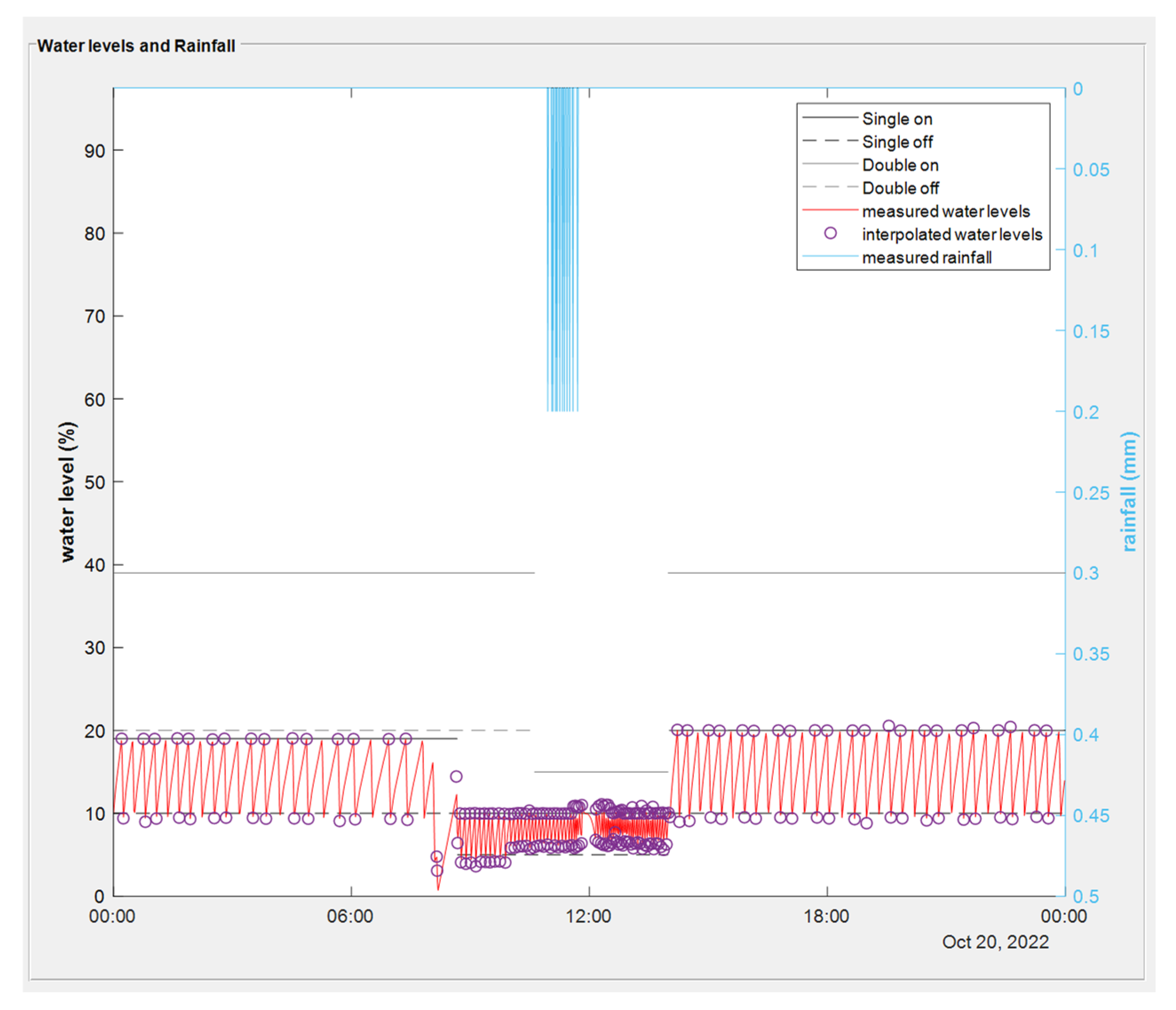
Figure A4 shows an example (for pumping station “Wauberg”) of preprocessed pump switch and level data with the identification of regime and regime change per cycle and the interpolated switch levels versus the expected ones. As can be seen, this is a day with some rain in the first hours as a result of which a number of cycles cannot be considered dry weather cycles. These non-dry weather cycles will not be used further in the cycle-based flow calculations.
Figure A4.
Example of data preprocessing.

Figure A5 shows the importance of keeping a history of the switch levels or having reliable interpolated levels to derive the switch levels if their history is not available. As can be seen from this example (from pumping station “Wijgmaalsesteenweg”), switch levels were temporarily lowered because of maintenance. If this information were not available and if no interpolated levels could be calculated, the incoming flows for those particular cycles would be significantly overestimated as a result of a wrongly assumed cycle volume (in this case, 6.1 m3 instead of 3.4 m3).
Figure A5.
Effect of variation of switch levels.

Appendix D
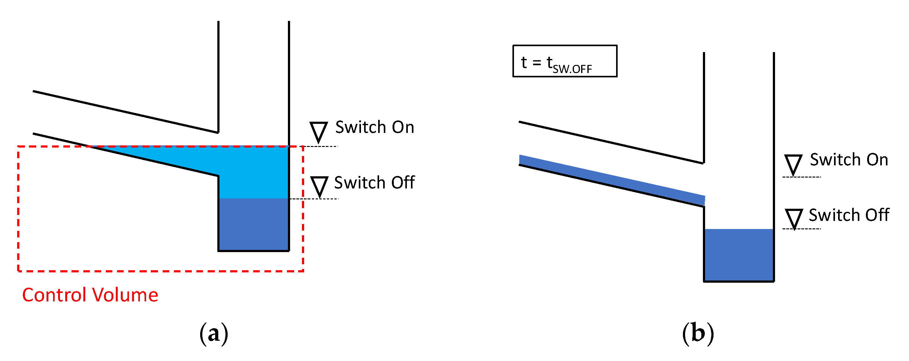
Even if the sizes and invert levels of the contributing pipes can be measured accurately, the classic assumption of a static storage-based control volume in the pipe (as shown in Figure A6a) is not physically correct. In such cases, the backwater curve of the incoming flow is permanently taking up a part of this theoretical static storage (as shown in Figure A6b). A better solution would be to delineate the control volume based on the intersection point between the switch-on level and the backwater curve. The (dead storage) volume under the curve between the intersection point and the wet well is then to be subtracted from the thus-obtained control volume (see Figure A6c).
Especially when the control volume extends far into the incoming network, such a calculation of the control volume can become quite complex, because the volume under the backwater curve is a function of the incoming flow.
Figure A6.
(a) Static storage-based delineation (left); (b,c) backwater curve-based delineation (right top and right bottom). The dark blue volumes are considered dead storage; the light blue ones are active storage.
Figure A6.
(a) Static storage-based delineation (left); (b,c) backwater curve-based delineation (right top and right bottom). The dark blue volumes are considered dead storage; the light blue ones are active storage.


References
- Beheshti, M.; Sægrov, S. Detection of Extraneous Water Ingress into the Sewer System Using Tandem Methods—A Case Study in Trondheim City. Water Sci. Technol. 2019, 79, 231–239. [Google Scholar] [CrossRef] [PubMed]
- Dakša, G.; Dejus, S.; Rubulis, J. Assessment of Infiltration from Private Sewer Laterals: Case Study in Jurmala, Latvia. Water 2022, 14, 2870. [Google Scholar] [CrossRef]
- Jenssen Sola, K.; Bjerkholt, J.; Lindholm, O.; Ratnaweera, H. Infiltration and Inflow (I/I) to Wastewater Systems in Norway, Sweden, Denmark, and Finland. Water 2018, 10, 1696. [Google Scholar] [CrossRef] [Green Version]
- Diem, J.E.; Pangle, L.A.; Milligan, R.A.; Adams, E.A. How Much Water Is Stolen by Sewers? Estimating Watershed-Level Inflow and Infiltration throughout a Metropolitan Area. J. Hydrol. 2022, 614, 128629. [Google Scholar] [CrossRef]
- Dirckx, G.; Bixio, D.; Thoeye, C.; De Gueldre, G.; Van De Steene, B. Dilution of Sewage in Flanders Mapped with Mathematical and Tracer Methods. Urban Water J. 2009, 6, 81–92. [Google Scholar] [CrossRef]
- Dirckx, G.; Fenu, A.; Wambecq, T.; Kroll, S.; Weemaes, M. Dilution of Sewage: Is It, after All, Really Worth the Bother? J. Hydrol. 2019, 571, 437–447. [Google Scholar] [CrossRef]
- Bentes, I.; Silva, D.; Vieira, C.; Matos, C. Inflow Quantification in Urban Sewer Networks. Hydrology 2022, 9, 52. [Google Scholar] [CrossRef]
- Ohlin Saletti, A.; Lindhe, A.; Söderqvist, T.; Rosén, L. Cost to Society from Infiltration and Inflow to Wastewater Systems. Water Res. 2023, 229, 119505. [Google Scholar] [CrossRef]
- Rezaee, M.; Tabesh, M. Effects of Inflow, Infiltration, and Exfiltration on Water Footprint Increase of a Sewer System: A Case Study of Tehran. Sustain. Cities Soc. 2022, 79, 103707. [Google Scholar] [CrossRef]
- Franz, T. Spatial Classification Methods for Efficient Infiltration Measurements and Transfer of Measuring Results. Ph.D. Thesis, Technische Universität Dresden, Dresden, Germany, 2007. [Google Scholar]
- Guo, S.; Ding, R.; Huang, B.; Zhu, D.Z.; Zhou, W.; Li, M. Experimental Study on Three Simple Tracers for the Assessment of Extraneous Water into Sewer Systems. Water Sci. Technol. 2022, 85, 633–644. [Google Scholar] [CrossRef]
- Guo, S.; Shi, X.; Luo, X.; Yang, H. River Water Intrusion as a Source of Inflow into the Sanitary Sewer System. Water Sci. Technol. 2020, 82, 2472–2481. [Google Scholar] [CrossRef] [PubMed]
- Heiderscheidt, E.; Tesfamariam, A.; Marttila, H.; Postila, H.; Zilio, S.; Rossi, P.M. Stable Water Isotopes as a Tool for Assessing Groundwater Infiltration in Sewage Networks in Cold Climate Conditions. J. Environ. Manag. 2022, 302, 114107. [Google Scholar] [CrossRef] [PubMed]
- Zhang, M.; Liu, Y.; Dong, Q.; Hong, Y.; Huang, X.; Shi, H.; Yuan, Z. Estimating Rainfall-Induced Inflow and Infiltration in a Sanitary Sewer System Based on Water Quality Modelling: Which Parameter to Use? Environ. Sci. Water Res. Technol. 2018, 4, 385–393. [Google Scholar] [CrossRef]
- De Bénédittis, J.; Bertrand-Krajewski, J.-L. Measurement of Infiltration Rates in Urban Sewer Systems: Use of Oxygen Isotopes. Water Sci. Technol. 2005, 52, 229–237. [Google Scholar] [CrossRef]
- Kracht, O.; Gresch, M.; Gujer, W. A Stable Isotope Approach for the Quantification of Sewer Infiltration. Environ. Sci. Technol. 2007, 41, 5839–5845. [Google Scholar] [CrossRef]
- Beheshti, M. Application of Infrastructure Asset Management in Enhancing the Performance of Sewer Networks. Ph.D. Thesis, Norwegian University of Science and Technology: Trondheim, Norway, 2019. [Google Scholar]
- Thapa, J.B.; Jung, J.K.; Yovichin, R.D. A Qualitative Approach to Determine the Areas of Highest Inflow and Infiltration in Underground Infrastructure for Urban Area. Adv. Civ. Eng. 2019, 2019, 2620459. [Google Scholar] [CrossRef]
- Schilperoort, R.; Hoppe, H.; de Haan, C.; Langeveld, J. Searching for Storm Water Inflows in Foul Sewers Using Fibre-Optic Distributed Temperature Sensing. Water Sci. Technol. 2013, 68, 1723–1730. [Google Scholar] [CrossRef]
- Beheshti, M.; Sægrov, S. Quantification Assessment of Extraneous Water Infiltration and Inflow by Analysis of the Thermal Behavior of the Sewer Network. Water 2018, 10, 1070. [Google Scholar] [CrossRef] [Green Version]
- Panasiuk, O.; Hedström, A.; Langeveld, J.; de Haan, C.; Liefting, E.; Schilperoort, R.; Viklander, M. Using Distributed Temperature Sensing (DTS) for Locating and Characterising Infiltration and Inflow into Foul Sewers before, during and after Snowmelt Period. Water 2019, 11, 1529. [Google Scholar] [CrossRef] [Green Version]
- Panasiuk, O.; Hedström, A.; Langeveld, J.; Viklander, M. Identifying Sources of Infiltration and Inflow in Sanitary Sewers in a Northern Community: Comparative Assessment of Selected Methods. Water Sci. Technol. 2022, 86, 1–16. [Google Scholar] [CrossRef]
- Beheshti, M.; Sægrov, S.; Ugarelli, R. Infiltration/Inflow Assessment and Detection in Urban Sewer System. Vann J. 2015, 1, 24–34. [Google Scholar]
- Karpf, C.; Hoeft, S.; Scheffer, C.; Fuchs, L.; Krebs, P. Groundwater Infiltration, Surface Water Inflow and Sewerage Exfiltration Considering Hydrodynamic Conditions in Sewer Systems. Water Sci. Technol. 2011, 63, 1841–1848. [Google Scholar] [CrossRef]
- Sowby, R.B.; Jones, D.R. A Practical Statistical Method to Differentiate Inflow and Infiltration in Sanitary Sewer Systems. J. Environ. Eng. 2022, 148, 06021006. [Google Scholar] [CrossRef]
- ATV-DVWK. Arbeitsblatt ATV-DVWK-A 198, Vereinheitlichung und Herleitung von Bemessungswerten für Abwasseranlagen (Standardisation and Derivation of Dimensioning Values for Wastewater Facilities); ATV-DVWK Deutsche Vereinigung für Wasserwirtschaft, Abwasser und Abfall e.V.: Hennef, Germany, 2003; Volume Band A 198. [Google Scholar]
- Weiß, G.; Brombach, H.; Haller, B. Infiltration and Inflow in Combined Sewer Systems: Long-Term Analysis. Water Sci. Technol. 2002, 45, 11–19. [Google Scholar] [CrossRef]
- Zhang, K.; Parolari, A.J. Impact of Stormwater Infiltration on Rainfall-Derived Inflow and Infiltration: A Physically Based Surface–Subsurface Urban Hydrologic Model. J. Hydrol. 2022, 610, 127938. [Google Scholar] [CrossRef]
- Jayasooriya, M.; Dahlhaus, P.; Vic, M.H.; Barton, A.; Gell, P. An Assessment of the Monitoring Methods and Data Limitations for Inflow and Infiltration in Sewer Networks. In Proceedings of the 36th HWRS: The Art and Science of Water, Hobart, Australia, 7–10 December 2015; Engineers Australia: Hobart, Australia, 2015. [Google Scholar]
- Bogusławski, B.; Sobczak, P.; Głowacka, A. Assessment of Extraneous Water Inflow in Separate Sewerage System by Different Quantitative Methods. Appl. Water Sci. 2022, 12, 278. [Google Scholar] [CrossRef]
- De Bénédittis, J.; Bertrand-Krajewski, J.-L. Infiltration in Sewer Systems: Comparison of Measurement Methods. Water Sci. Technol. 2005, 52, 219–227. [Google Scholar] [CrossRef] [PubMed]
- Sola, K.J.; Bjerkholt, J.T.; Lindholm, O.G.; Ratnaweera, H. Analysing Consequences of Infiltration and Inflow Water (I/I-Water) Using Cost-Benefit Analyses. Water Sci. Technol. 2020, 82, 1312–1326. [Google Scholar] [CrossRef]
- Ohlin Saletti, A.; Rosén, L.; Lindhe, A. Framework for Risk-Based Decision Support on Infiltration and Inflow to Wastewater Systems. Water 2021, 13, 2320. [Google Scholar] [CrossRef]
- Tomperi, J.; Rossi, P.M.; Ruusunen, M. Estimation of Wastewater Flowrate in a Gravitational Sewer Line Based on a Low-Cost Distance Sensor. Water Pract. Technol. 2022, 18, 40–52. [Google Scholar] [CrossRef]
- Bertrand-Krajewski, J.-L.; Clemens-Meyer, F.; Lepot, M. (Eds.) Metrology in Urban Drainage and Stormwater Management: Plug and Pray; IWA Publishing: London, UK, 2021; ISBN 978-1-78906-011-9. [Google Scholar]
- Fencl, M.; Grum, M.; Borup, M.; Mikkelsen, P.S. Robust Model for Estimating Pumping Station Characteristics and Sewer Flows from Standard Pumping Station Data. Water Sci. Technol. 2019, 79, 1739–1745. [Google Scholar] [CrossRef] [PubMed]
- Zhang, Z.; Laakso, T.; Wang, Z.; Pulkkinen, S.; Ahopelto, S.; Virrantaus, K.; Li, Y.; Cai, X.; Zhang, C.; Vahala, R.; et al. Comparative Study of AI-Based Methods—Application of Analyzing Inflow and Infiltration in Sanitary Sewer Subcatchments. Sustainability 2020, 12, 6254. [Google Scholar] [CrossRef]
- Matlab, 2019; The MathWorks, Inc.: Natick, MA, USA, 2019.
Figure 1.
General flowchart of the proposed methodology.

Figure 2.
Schematic representation of a pumping station, indicating the dry weather control volume.

Figure 3.
Detailed flowchart of the iterative flow calculation algorithm.

Figure 4.
Linearisation of incoming flows.

Figure 5.
Calculation of phase-out time.

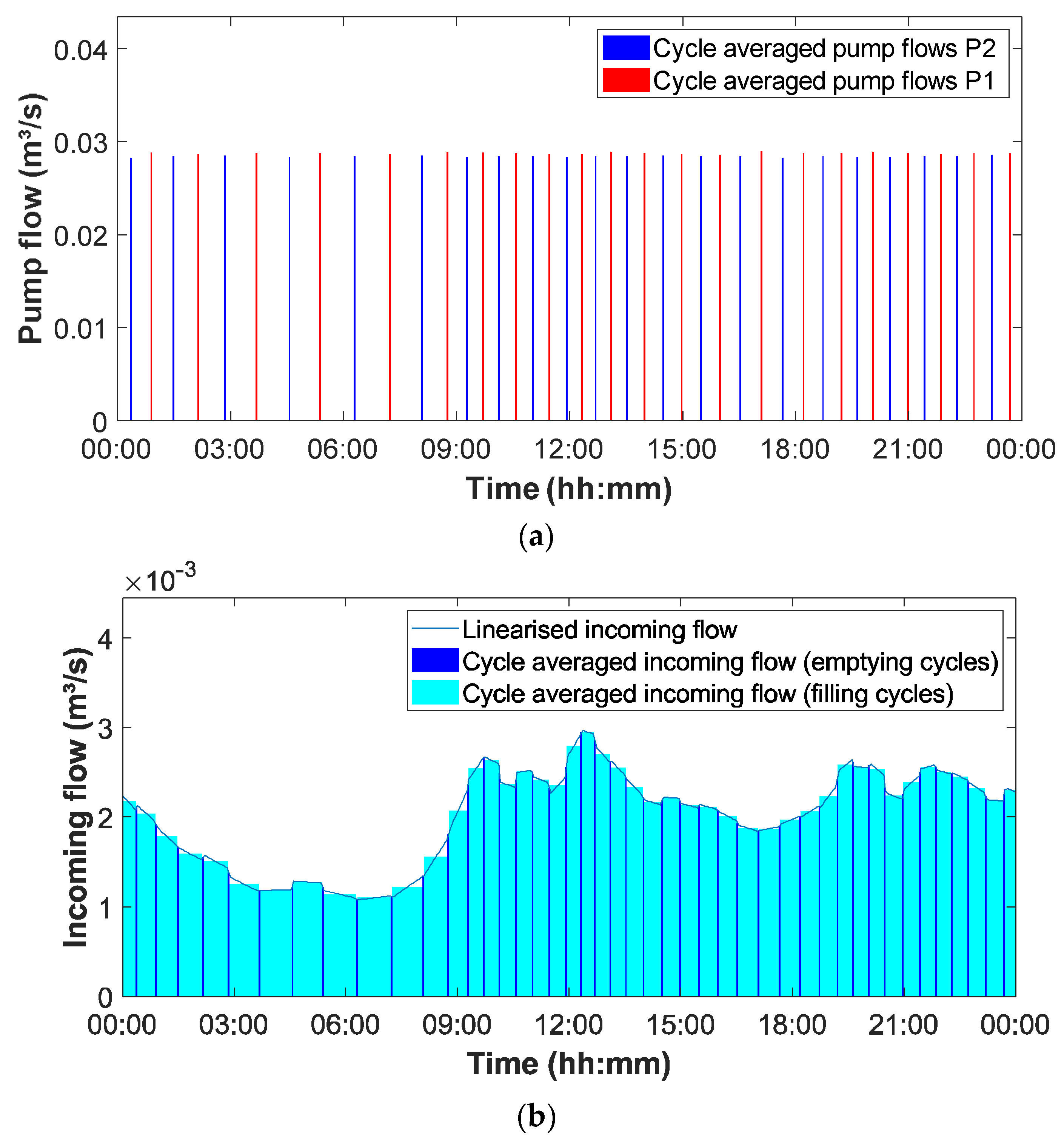
Figure 6.
Example of individual cycles’ flows: (a) pumped flows per cycle per pump (top); (b) average incoming flows for filling and emptying cycles and linearised flows for all cycles (bottom) (PS Zuidstraat).
Figure 6.
Example of individual cycles’ flows: (a) pumped flows per cycle per pump (top); (b) average incoming flows for filling and emptying cycles and linearised flows for all cycles (bottom) (PS Zuidstraat).

Figure 7.
Example of calculated pump flows with pumps of different nominal capacities: (a) pumped flows per cycle per pump (top); (b) average incoming flows for filling and emptying cycles and linearised flows for all cycles (bottom) (PS Wauberg).
Figure 7.
Example of calculated pump flows with pumps of different nominal capacities: (a) pumped flows per cycle per pump (top); (b) average incoming flows for filling and emptying cycles and linearised flows for all cycles (bottom) (PS Wauberg).


Figure 8.
Effect of missing pump loggings on the calculated cycle flows: (a) pumped flows per cycle per pump (top); (b) average incoming flows for filling and emptying cycles and linearised flows for all cycles (bottom) (PS Wijgmaalsesteenweg).
Figure 8.
Effect of missing pump loggings on the calculated cycle flows: (a) pumped flows per cycle per pump (top); (b) average incoming flows for filling and emptying cycles and linearised flows for all cycles (bottom) (PS Wijgmaalsesteenweg).

Figure 9.
Calculated vs. measured pump flows before (a) and after (b) control volume correction (PS Vuntlaan).
Figure 9.
Calculated vs. measured pump flows before (a) and after (b) control volume correction (PS Vuntlaan).

Figure 10.
Overview of daily incoming volumes: (a) only dry weather days (top); (b) all days including rainfall for the selected period (bottom) (PS Zuidstraat).
Figure 10.
Overview of daily incoming volumes: (a) only dry weather days (top); (b) all days including rainfall for the selected period (bottom) (PS Zuidstraat).

Figure 11.
Calculated incoming flows at the start and end of a dry period with high initial infiltration (PS Zuidstraat).
Figure 11.
Calculated incoming flows at the start and end of a dry period with high initial infiltration (PS Zuidstraat).

Figure 12.
Example of the impact of a construction site’s pumped groundwater drainage. The inflow period extends from 22 June 2022 to 22 July 2022. (PS Wauberg).
Figure 12.
Example of the impact of a construction site’s pumped groundwater drainage. The inflow period extends from 22 June 2022 to 22 July 2022. (PS Wauberg).

Disclaimer/Publisher’s Note: The statements, opinions and data contained in all publications are solely those of the individual author(s) and contributor(s) and not of MDPI and/or the editor(s). MDPI and/or the editor(s) disclaim responsibility for any injury to people or property resulting from any ideas, methods, instructions or products referred to in the content. |
© 2023 by the authors. Licensee MDPI, Basel, Switzerland. This article is an open access article distributed under the terms and conditions of the Creative Commons Attribution (CC BY) license (https://creativecommons.org/licenses/by/4.0/).
Share and Cite
MDPI and ACS Style
Van Assel, J.; Kroll, S.; Delgado, R. Calculation of Dry Weather Flows in Pumping Stations to Identify Inflow and Infiltration in Urban Drainage Systems. Water 2023, 15, 864. https://doi.org/10.3390/w15050864
AMA Style
Van Assel J, Kroll S, Delgado R. Calculation of Dry Weather Flows in Pumping Stations to Identify Inflow and Infiltration in Urban Drainage Systems. Water. 2023; 15(5):864. https://doi.org/10.3390/w15050864
Chicago/Turabian StyleVan Assel, Johan, Stefan Kroll, and Rosalia Delgado. 2023. "Calculation of Dry Weather Flows in Pumping Stations to Identify Inflow and Infiltration in Urban Drainage Systems" Water 15, no. 5: 864. https://doi.org/10.3390/w15050864
Note that from the first issue of 2016, this journal uses article numbers instead of page numbers. See further details here.