

Remote-Sensing Extraction of Small Water Bodies on the Loess Plateau

1
College of Natural Resources and Environment, Northwest A&F University, Yangling 712100, China
2
The Academy of Digital China, Fuzhou University, Fuzhou 350108, China
3
Inner Mongolia Water Resources and Hydropower Survey and Design Institute Co., Ltd., Hohhot 010020, China
4
Water Resources Development Center, Water Resources Bureau of Jungar Banner, Ordos City 010300, China
*
Author to whom correspondence should be addressed.
Water 2023, 15(5), 866; https://doi.org/10.3390/w15050866
Submission received: 7 January 2023
/
Revised: 10 February 2023
/
Accepted: 20 February 2023
/
Published: 23 February 2023
(This article belongs to the Special Issue Remote Sensing-Based Study on Surface Water Environment)
Abstract
:The mixed pixel of low-resolution remote-sensing image makes the traditional water extraction method not effective for small water body extraction. This study takes the Loess Plateau with complex terrain as the research area and develops a multi-index fusion threshold segmentation algorithm (MFTSA) for a large-scale small water body extraction algorithm based on GEE (Google Earth Engine). MFTSA uses the AWEI (automated water extraction index), MNDWI (modified normalized difference water index), NDVI (normalized difference vegetation index) and EVI (enhanced vegetation index) for multi-index synergy to extract small water bodies. It also uses slope data generated by the SRTM (Shuttle Radar Topography Mission digital elevation model) and NIR band reflectance to eliminate suppressing high reflectivity noise and shadow noise. An MFTSA algorithm was proposed and the results showed that: (1) The overall extraction accuracy of the MFTSA algorithm on the Loess Plateau was 98.14%, and the correct extraction rate of small water bodies was 92.82%. (2) Compared with traditional water index methods and classification methods, the MFTSA algorithm could extract small water bodies with higher integrity and clearer and more accurate boundaries. (3) The MFTSA algorithm was used to extract a total of 69,900 small water bodies on the Loess Plateau, accounting for 97.63% of the total water bodies, and the area was 482.11 square kilometers, accounting for 16.50% of the total water bodies.
1. Introduction
A small water body is an important component of a terrestrial ecosystem. Compared with large water bodies, small water bodies are more widely distributed and play an important role in the local ecology for the diversity of freshwater organisms. However, small water bodies are often ignored in resource surveys, resulting in a lack of a comprehensive understanding of their spatial distribution, which limits water resource utilization [1,2]. Currently, there is no uniform definition for small water bodies. Jiang et al. [3] defined small water bodies as narrow water bodies whose apparent width in an image is less than or equal to three pixels. Biggs et al. [1] defined small water bodies as sets of ponds and small lakes, low streams, ditches and springs. In this study, water bodies with an area of less than 0.1 km2 are defined as small water bodies, mainly including ponds, aquaculture water surfaces, ditches, artificial water reservoirs, small reservoirs, small rivers, etc.
Water body extraction methods can be divided into three basic types in optical remote sensing [4]: the single-threshold segmentation method, multi-band spectral relationship method and classification method. The single-threshold segmentation method is simple. It mainly uses the difference in the spectral characteristics of a water body and other ground objects in certain bands to extract the water body. The threshold selection criterion directly determines the accuracy of water body extraction. This method is effective in extracting large water bodies such as lakes and rivers but not effective in study areas with more mixed pixels of water and non-water, so the extraction effect in mountainous areas and small water bodies is not ideal [5]. The multi-band spectral relation method mainly uses the difference of spectral characteristics to distinguish water bodies from other ground objects. This method is more suitable for areas with small terrain fluctuations [6,7]. The classification method extracts small water bodies by spectral, spatial and texture features of images. The commonly used classifiers include the support vector machine (SVM), decision tree and so on. The classification method has high accuracy in extracting water bodies but is significantly affected by samples, which can be easily confused by ice, snow and mountain shadows [8,9].
Currently, most water body extraction methods are only effective for large water areas and are not suitable for small water bodies. Small water bodies show small and narrow spatial characteristics on low-resolution images, and the spectral features are complex. The water–land boundaries extracted by different methods may have the phenomenon of edge loss or river flow interruption. The features of small water bodies in different regions on the Loess Plateau are not exactly the same. Some rivers have no flow during the dry season, and many large water bodies significantly reduce its surface area. These water bodies contain a lot of sediment, and the spectral characteristics of water bodies are weakened. Therefore, the spectral features of water bodies in different places are quite different. In addition, there are many mountain shadows on the Loess Plateau, and these shadows cause serious noise in the extraction of small water bodies. In this case, by using the same model and parameters for the Loess Plateau images it is difficult to extract all water bodies, and it is even more difficult to obtain very accurate water surface edges.
In view of the above problems, the main objective of this study was (1) to develop a simple algorithm model for small water bodies’ extraction on the Loess Plateau that takes into account the relationship between multi-band spectra; (2) to verify the accuracy of the multi-index fusion threshold segmentation algorithm (MFTSA) and water index method and classification method; (3) to extract small water bodies by GEE from the Landsat5 remote-sensing images of the Loess Plateau acquired in 2010. The research results can provide scientific reference for the ecological protection of the Loess Plateau and the sustainable utilization of regional water resources.
2. Study Area and Data Source
2.1. Study Area
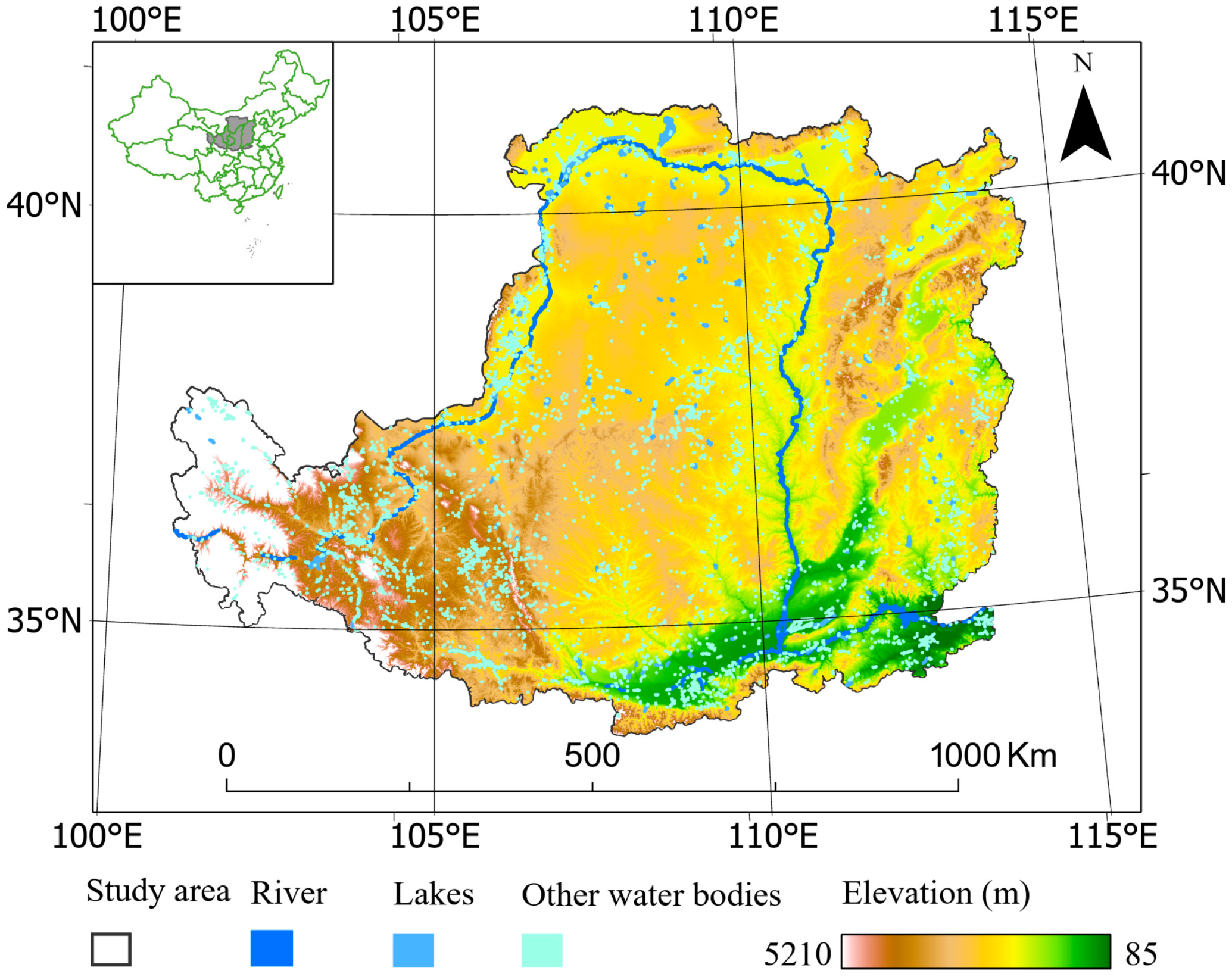
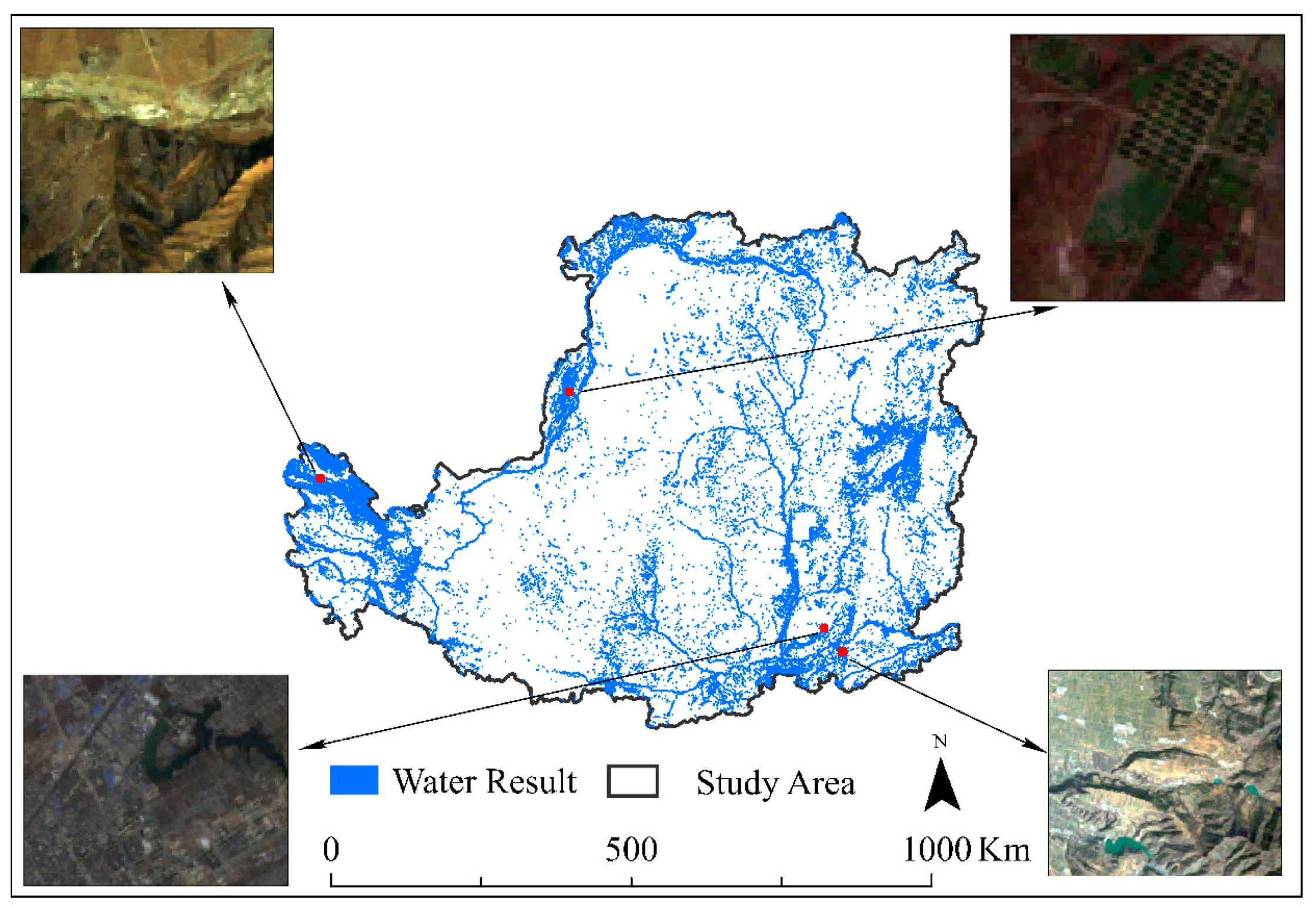
The Loess Plateau is located in the north-central part of China, with a total area of about 640,000 km2. It is the largest loess sedimentary region in the world (Figure 1). The strong water erosion on the Loess Plateau not only reduces the fertility of the land but also leads to a continuous uplift of the riverbed and threat of the river to both sides of the downstream. The Yellow River is the main water system on the Loess Plateau region; the river has a high sand content. Due to the special hydrometeorological conditions and underlying surface conditions of the Loess Plateau, people have built a large number of check dams, small and medium-sized reservoirs, and cisterns. These reservoirs reduce the amount of sediment flowing into the river. There are a large number of small water bodies on the Loess Plateau, whose distribution is closely related to rainfall, topography and population distribution. The study of small water bodies on the Loess Plateau is of great significance for reducing soil erosion, increasing crop yields and improving the living environment.
2.2. Data Source
The main data of this study include: (1) The land cover data of the Loess Plateau in 2010 [10], the data resolution is 30 m. We generated random points on different land cover types of the data, then extracted pixel values of these random points, calculated the corresponding index values and finally drew scatter density maps of water and non-water bodies. In addition, these random points were used as training and test datasets when using the classifier to extract water bodies. (2) Landsat 5 TM remote image data. In Google Earth Engine (GEE), we screened images with cloud cover less than 5% for median synthesis as the original dataset for water extraction. After generating random points, we loaded Landsat 5 TM remote image data in GEE and deleted the sample points that were inconsistent between the actual category and the sample category. (3) The Shuttle Radar Topography Mission Digital Elevation Model (SRTM) [11] has a spatial resolution of 30 m and is mainly used to generate slope datasets and assist in eliminating shadow noise.
3. Research Methods
3.1. New Water Extraction Method Uses Multiple Remote-Sensing Water Indices
3.1.1. New Water Extraction Method
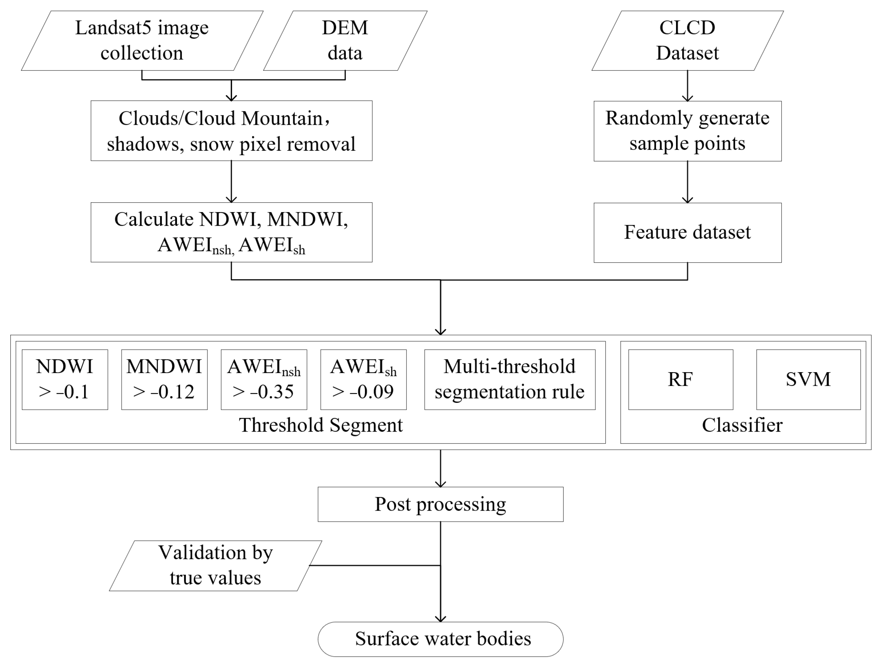
A schematic of an analytical procedure of this research is shown in Figure 2. The Landsat TM image dataset and DEM data on GEE were obtained, and the pixels such as clouds, shadows, ice and snow in the image were removed. There are many mountain shadows in the study area, and these shadows have large slopes. In this study, pixels with a slope greater than 20° were removed to minimize the impact of mountain shadows on water extraction. To eliminate the influence of ice and snow and some high-reflectivity ground objects within the urban development area, the near-infrared band (NIR) was selected to eliminate the high-reflectivity noise pixels with reflectivity greater than 0.2 [12]. In order to compare different methods, we evaluated the accuracy of water extraction results of different methods and further processed the water extraction results to get a small-water-distribution map on the Loess Plateau.
3.1.2. Extraction of Small Water Body by a Single Remote-Sensing Index
The process of single-band threshold method for water extraction is as follows: spectral values between water body and non-water body are analyzed to set band segmentation threshold for water extraction. Those indices include the normalized difference water index (NDWI) [13], the modified normalized difference water index (MNDWI) [14] and the automated water extraction index (AWEI) [15]. The AWEI index consists of two indices: one for images with no shadow () and another for those with shadows from mountains, buildings and clouds () [15]. The calculation formula is shown in Table 1. The single-band threshold method uses the minimum error threshold, entropy threshold or Otsu [16] threshold segmentation method to extract the water body.
In the process of remote-sensing-image classification, the accuracy and typicality of sample selection directly affects classification accuracy. Therefore, a stratified sampling method was adopted in this study, and sample selection was carried out in accordance with the principles of sample quantity requirements, sample representativeness and difference. In this study, it was stratified random sampling generated from the 2010 China’s land cover dataset (CLCD) [10]. A Landsat5 TM image was used, including a total of 21,725 water body sample points and 51,485 non-water body sample points (1807 impervious sample points, 871 snow points, 6762 forest points, 14,797 cultivated points, 2095 bare points, and 25,153 grassland points). We calculated the NDWI, MNDWI and AWEI and determined the threshold where the density of water bodies and non-water bodies intersected.
3.1.3. Multi-Exponential Fusion Threshold Segmentation for Small Water Body Extraction
Single-exponential segmentation often has low accuracy in water body identification because it is difficult to determine the ideal segmentation threshold. Dong found that water extraction rules built according to the relationship between the water body index and vegetation index could extract a water body better [17]. Researchers first calculated the MNDWI, enhanced vegetation index (EVI) [7] and normalized difference vegetation index (NDVI) [18] values of each pixel in the study area and then constructed water extraction rules of MNDWI > EVI or MNDWI > NDVI according to the spectral index distribution of sample points. This rule classifies pixels whose water signals are stronger than vegetation signals as water bodies. Deng [19] drew a scatter density map between the water body index and the vegetation index and found that water body pixels and non-water body pixels can be distinguished by constructing a threshold segmentation rule for multiple remote-sensing indices. Based on the above studies, this study firstly calculated the AWEI, MNDWI, EVI and NDVI values of samples, then found the distribution rules between water and non-water in different indices by drawing the scatter density of water and non-water sample points and finally determined the extraction rules of small water bodies on the Loess Plateau.
3.2. Classification Method to Extract Small Water Bodies
3.2.1. Selection of Input Data
The Loess Plateau land cover is classified into seven types: impermeable surface (including buildings, roads, mountains, abandoned land, etc.), farmland, bare land, forest land, grassland, snow and water body. There are seven bands in the Landsat5 image, as shown in Table 2. The Blue band is more sensitive to water bodies, the green band has higher reflectivity in surface water bodies, the red band is often used to distinguish the types of man-made features and the NIR band has the highest reflectivity in non-water bodies. This is a theoretical basis for construct vegetation indices and water body indices [13,14,15]. The SWIR1 band can be used to detect plant water content and soil humidity, and LWIR can be used to detect land surface temperature. The SWIR2 band can be used to detect hydrothermal altered rocks associated with mineral deposits. To improve the classification accuracy, we added all seven bands to the feature dataset. The classifier could easily confuse a water body and a shadow, and the slope of a shadow is generally larger than that of a water body [20]. Therefore, the slope data was selected for the input dataset.
The vegetation index can enhance vegetation information, and the water body index can identify water body information. Adding the vegetation and water body indices to the feature dataset helps a classifier identify objects better [14,19]. In order to compare the effects of adding remote-sensing indices (MNDWI, EVI, NDVI and AWEI) on the classification of water bodies, we designed two sets of experiments, without indices and with indices, to explore whether adding these index features could improve the classification accuracy.
3.2.2. Classifier Selection
RF was developed by Breiman [21]. It uses bagging and feature randomness when building each individual tree to try to create an uncorrelated forest of trees whose prediction by committee is more accurate than that of any individual tree. The RF algorithm can improve the accuracy and generalization performance of the model by selecting different training samples and different features. It is fast in training and classification, can effectively process large amounts of data and has strong anti-noise ability. It is widely used in the field of remote-sensing image recognition and classification [22,23]. In this study, RF classifiers were trained in our application, increasing the number of trees from time to time (from 1 to 100) [24]. By analyzing the change in overall accuracy, we determined that the number of trees parameter was better set to 40. The other parameters of the RF model remained default.
SVM was developed by Cortes et al. [25]. SVM is a linear model for classification and regression problems. It can solve linear and nonlinear problems and work well for many practical problems. Zhang et al. proposed a posterior probabilistic SVM method [9] that uses five water-sensitive Landsat OLI bands and topographic indices as inputs to map river water bodies. Experiments show that water bodies extraction with this method is highly precise. The SVM classifier can consider the spectral, spatial and texture features of water for small water bodies’ extraction. In this study, we chose RBF as the kernel function type of the SVM model, because this kernel function is relatively stable. The values of gamma and cost of the SVM model were selected by an experimental trial method [24]. The SVM parameters we finally determined were Gamma = 10 and Cost = 25, and other parameters remained default.
3.3. Evaluation Method
To evaluate the results of different methods, we randomly selected 831 river sample points, 557 lake sample points, 790 reservoir sample points, 836 small water sample points, 1306 shadow sample points and 865 snow sample points in the study area as the test dataset. Finally, we used these sample points to calculate different indicators of different models. We chose user’s accuracy (UA), producer accuracy (PA), overall accuracy (OA), Kappa accuracy (Kappa) and small water extraction rate (SWER) as the evaluation index of the different methods. UA is defined as the probability of taking a random sample from the classification results, whose type can indeed represent the actual class. PA is defined as the probability that the actual sample is correctly classified. OA is the ratio between the number of correctly classified samples and the total number of samples. Kappa is used for the consistency test and can also be used to measure classification accuracy. SWER is the ratio of the correctly extracted small water bodies to the total small water bodies, which reflects the completeness of the extracted small water bodies.
4. Result
4.1. Small Water Extraction Based on Remote-Sensing Index
4.1.1. Determination of Remote-Sensing Index Segmentation Threshold
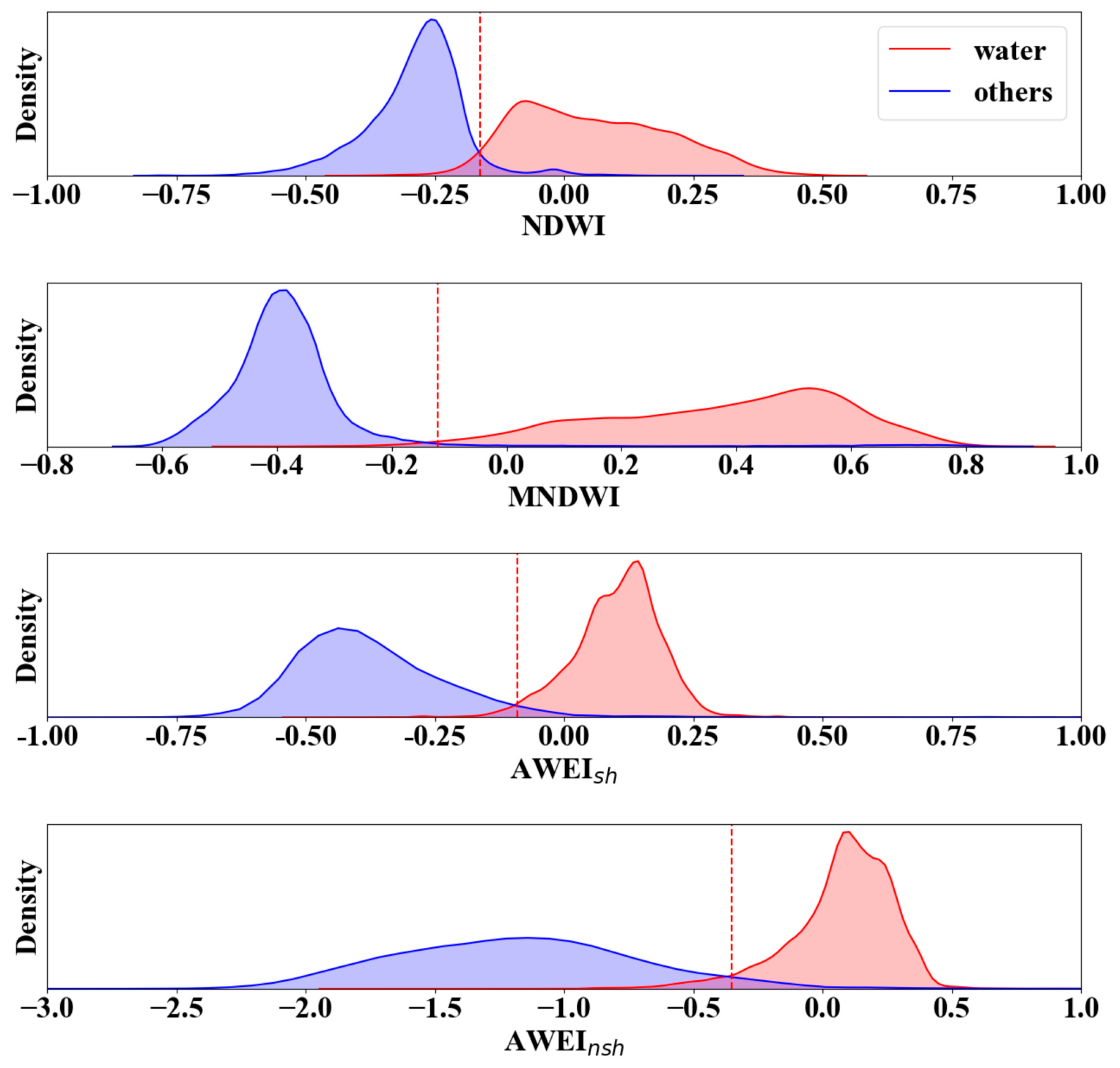
To explore the water index segmentation threshold, the remote-sensing indices of training sample points were calculated, and a density map is shown (Figure 3). We only extracted water bodies; non-water bodies were uniformly classified into others.
The peaks of water bodies and non-water bodies were significantly different (Figure 3). Most water information could be separated by NDWI, and , but there were overlapping pixels between water bodies and non-water bodies at the threshold segmentation. By comparison, the MNDWI method had good separability. There were few overlapping areas between water bodies and others. Finally, the segmentation thresholds of NDWI, MNDWI, and methods were −0.16, −0.12, −0.09, −0.35, respectively.
Based on the algorithm proposed by Zou et al. [26] and Deng et al. [19], this study firstly calculated the remote-sensing index of sample points, drew the scatter density map of water and non-water bodies (Figure 4) and determined the segmentation threshold according to the scatter density map.
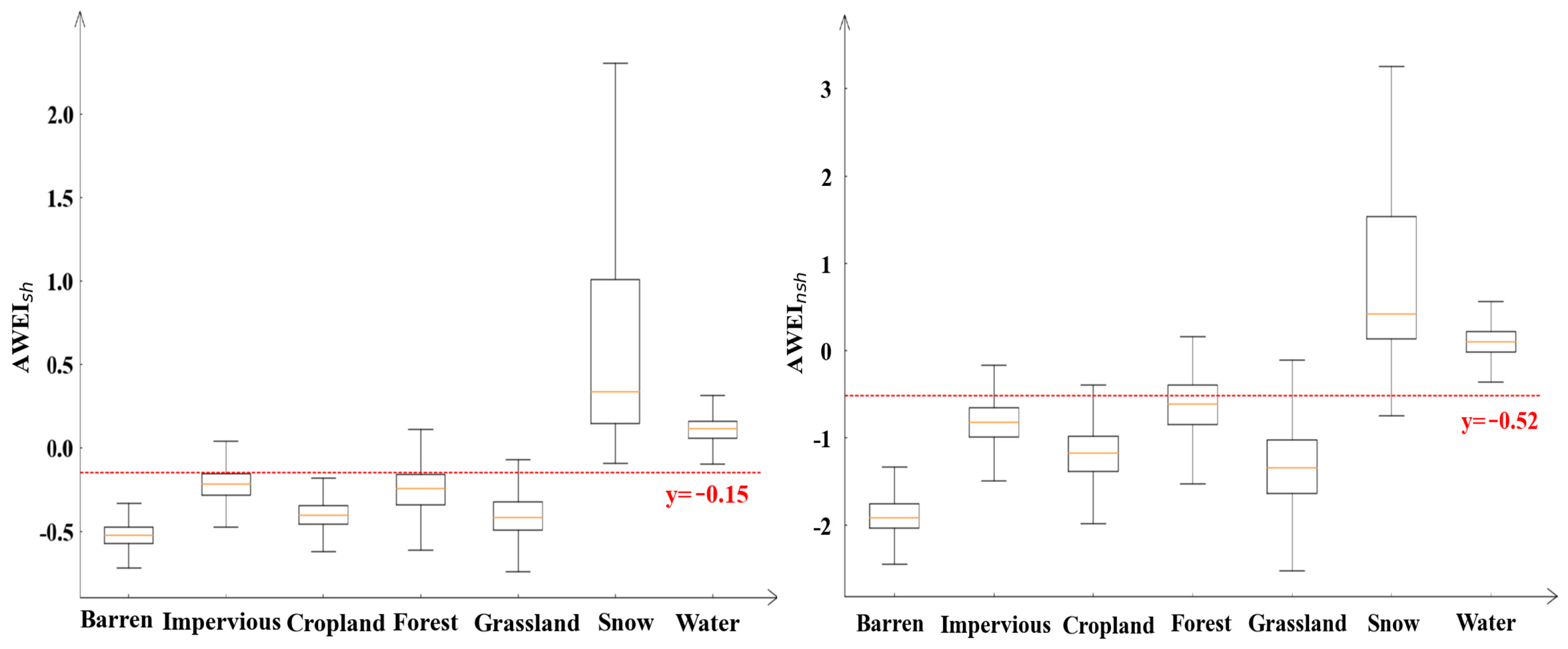
Training samples are concentrated in the first quadrant separated by the red dotted line, and the non-water body samples are concentrated in the third quadrant (Figure 4). The method misidentified 4.69% of water bodies as non-water bodies and 3.97% of non-water bodies as water bodies. To remove misclassified non-water bodies from water bodies, we used the AWEI index for threshold segmentation. To compare the differences between water bodies and other ground objects in the and , we drew a box plot (Figure 5). Except for snow, water bodies had good separability from other ground objects. When > −0.15 and > −0.52 were satisfied, the MFTSA method had a good effect on suppressing mixed-pixel and shadow noise. Finally, the MFTSA method (( > −0.15 and > −0.52) and () > −0.18 and (MNDWI-EVI > −0.25 or MNDWI-NDVI > −0.25)) was used to make a small-water-bodies map based on Landsat TM5 data of the Loess Plateau.
4.1.2. Analysis of Results of Small Water Bodies Extracted by Remote-Sensing Index Method
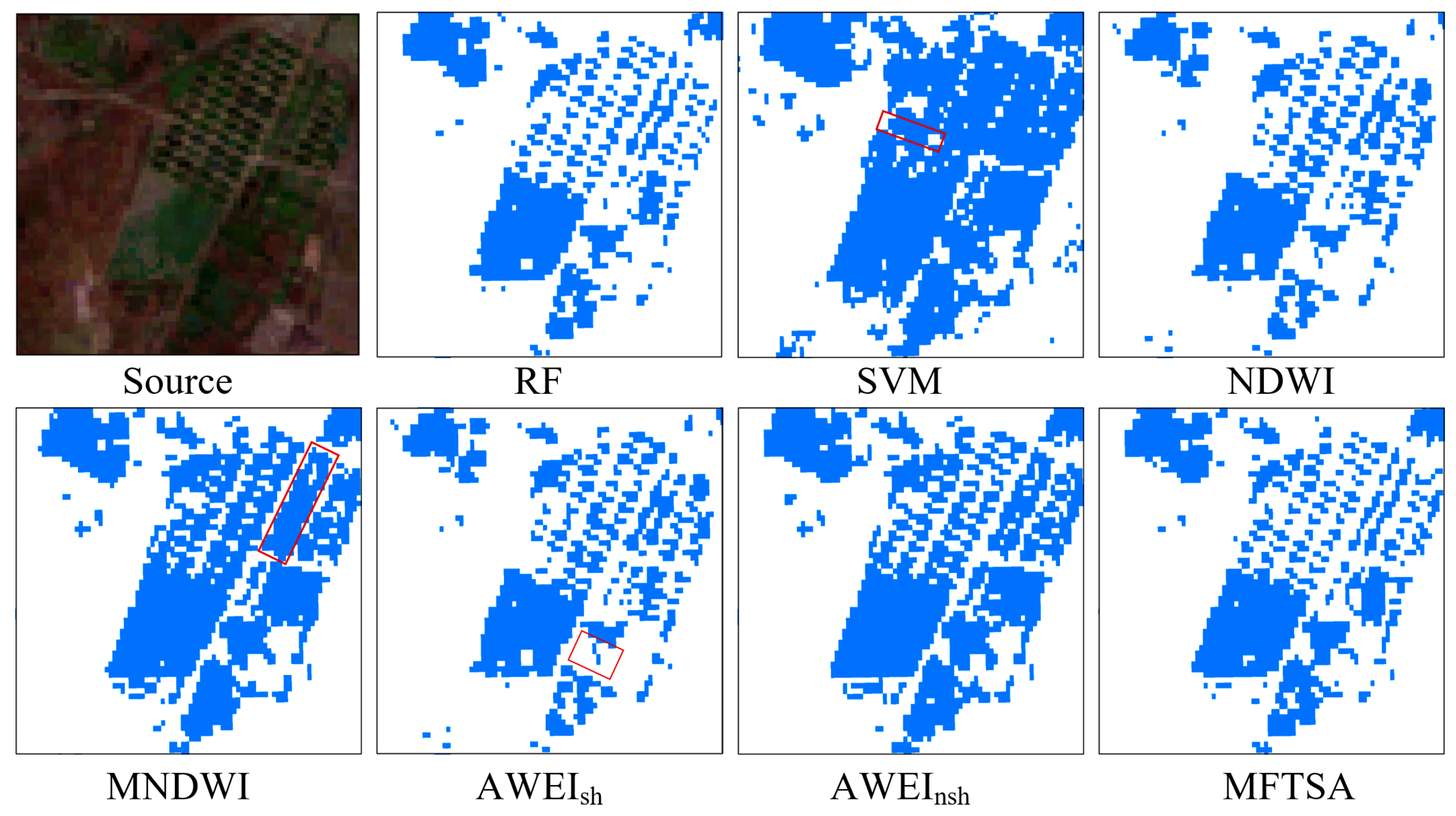
To compare the effects of different remote-sensing index methods in extracting small water bodies, five methods, namely NDVI, NDWI, MNDWI, , and MFTSA, were used to extract water bodies on the Loess Plateau. Three typical areas were selected that included small water bodies to display the extraction results in detail (Figure 6).
Study area (a) was a small ditch of uniform width. As shown in Figure 6, the MNDWI and methods identified some non-water pixels as water pixels around the ditch, and the two methods identified different ditch widths. By contrast, other methods could identify water body information more accurately. Study areas (b) and (c) were ponds. The NDWI, MNDWI, and had difficulties identifying the boundary between ponds, which led to fuzzy boundaries of ponds in the identification result. However, the MFTSA method showed clear pond boundaries and complete extraction of small water bodies. To quantitatively evaluate the influence of different remote-sensing indexes on small-water-bodies extraction, experimental datasets were used in this study to evaluate the accuracy of different methods. The correct extraction results and accuracy of different methods on the test dataset are shown in Table 3 and Table 4, respectively.
As shown in Table 3, NDWI could suppress snow and mountain shadow information and highlight water body features. However, only 69% of small water bodies were extracted by the NDWI method, and the OA index was only 87%. The MNDWI method suppressed residential and soil noise well, highlighted water body information and rarely leaked water bodies. The integrity of the MNDWI method in extracting large and small water bodies was high, and the SWER of this method was up to 92%. However, this method was easily affected by shadow, snow and mixed pixels, so it recognized non-water bodies such as snow, shadows, sediment and pond stalks as water bodies, which resulted in fuzzy boundaries of some water bodies in the identification results (Figure 6). The extraction effect of MNDWI was better in the relatively flat area in the middle part of the Loess Plateau, but it was less effective for the complex terrain. The method based on could remove hill shadow noise, but it had poor accuracy on urban impervious surface and some water pixels. The extraction accuracy of was good for large water bodies such as rivers, lakes and reservoirs but not ideal for small water bodies. The method based on could effectively eliminate dark buildings in urban background areas and non-water pixels such as snow, but this method missed more small water pixels. Although the UA index of this method was higher, the SWER index was only 64%. Among all the methods, the method had the lowest SWER index because it removed a part of the water bodies when removing background noise, which is consistent with the research results of Jiang et al. [3]. Small water bodies extracted by the MFTSA method had high integrity and clear boundaries (Figure 6), and there was better removal of shadow noise. Among all the methods, this method had the highest OA and SWER index.
4.2. Extraction of Small Water Bodies Based on Machine Learning Algorithms
4.2.1. Analysis of RF and SVM Accuracy for Extracted Small Water Bodies
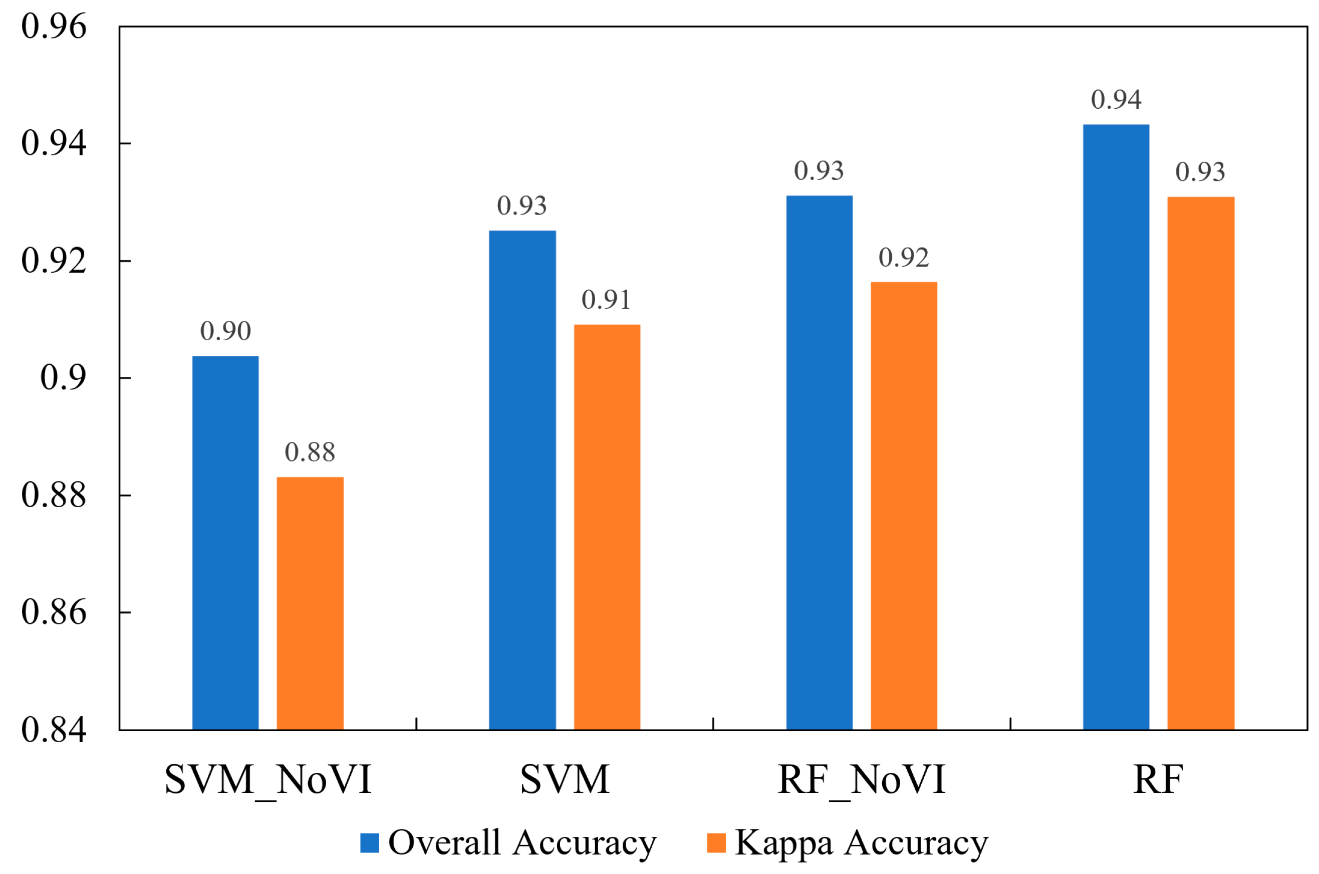
In this study, 73,210 samples were randomly divided into the training dataset and test dataset according to an 8:2 ratio. RF and SVM were used to train and test the dataset. The accuracy of different models is shown in Figure 7.
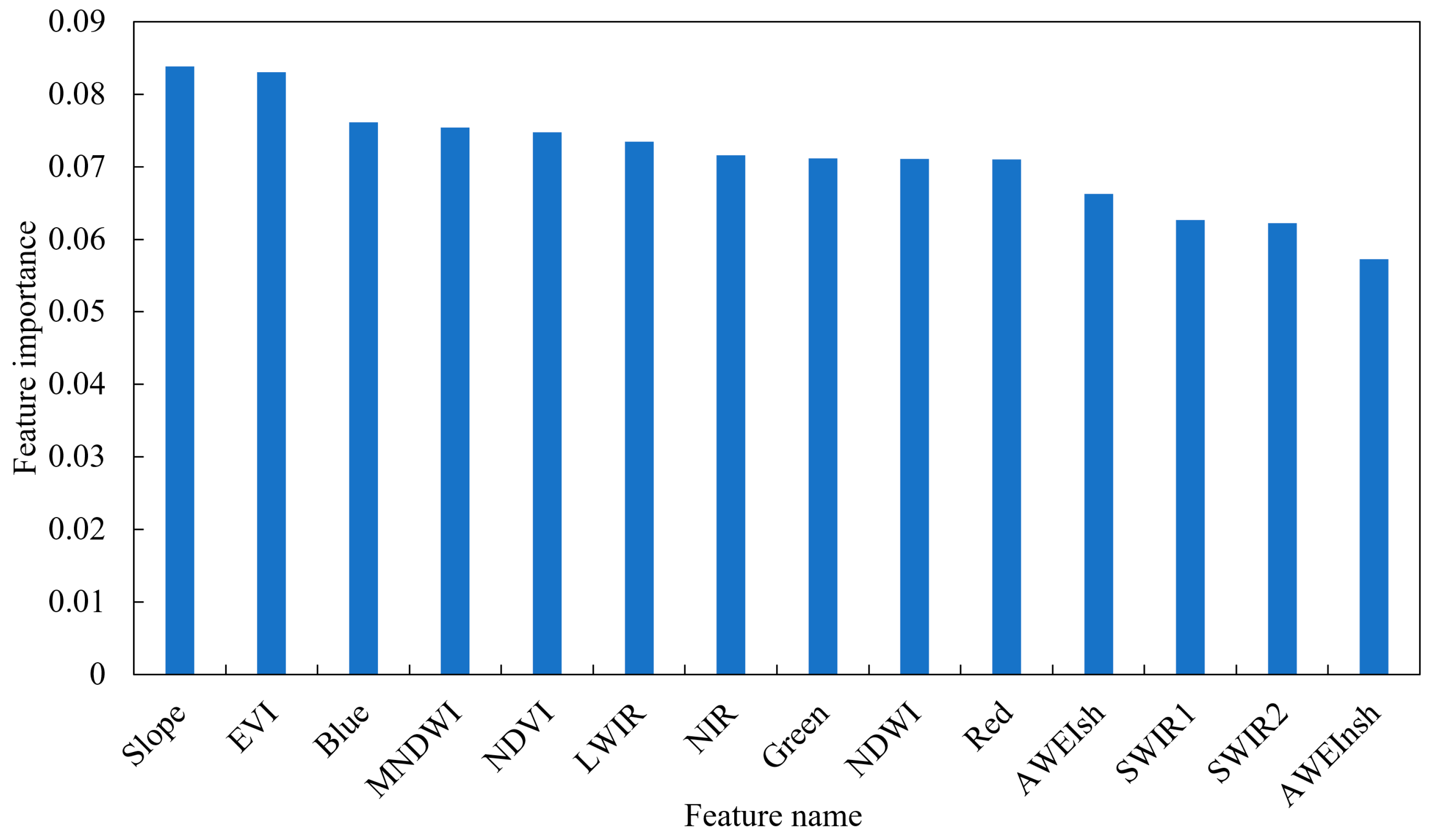
In Figure 7, RF_NoVI is the classification result obtained by using original Landsat5 bands and the slope band as the input dataset to train the RF model. RF is the classification result of adding NDVI, NDWI, MNDWI, and features to the original feature dataset. After adding those remote-sensing indices, the overall accuracy and Kappa accuracy of SVM and RF were improved. It can be seen that adding those indices could significantly improve the classification accuracy of water bodies. The feature importance of the RF model (Figure 8) indicated that Slope, EVI and Blue bands had higher feature importance.
As shown in Figure 8, the importance of Slope, EVI and Blue features was relatively high, which was mainly related to samples. The top three samples in the dataset were grassland, water and cultivated land. The three land cover types were all sensitive to slope, while grassland and cultivated land were sensitive to EVI, and the blue band was sensitive to water bodies. Therefore, the Slope, EVI, and Blue features were more important. Although was sensitive to water bodies, it was difficult for this index to distinguish grasslands, woodlands and cultivated land, so the importance of features was relatively low.
4.2.2. Analysis of Extraction Results of Different Classification Methods
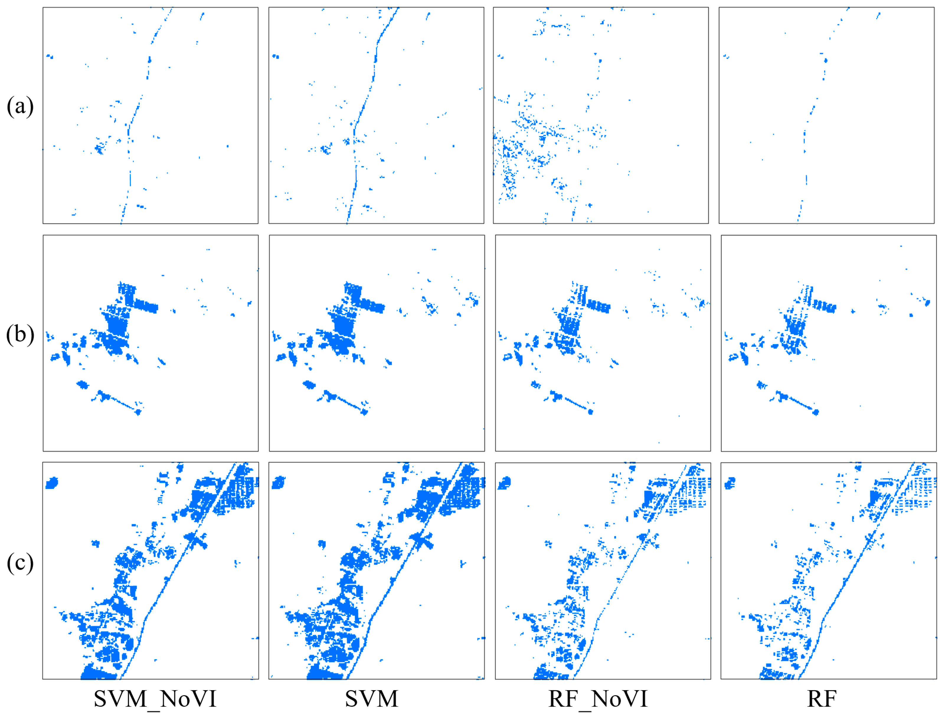
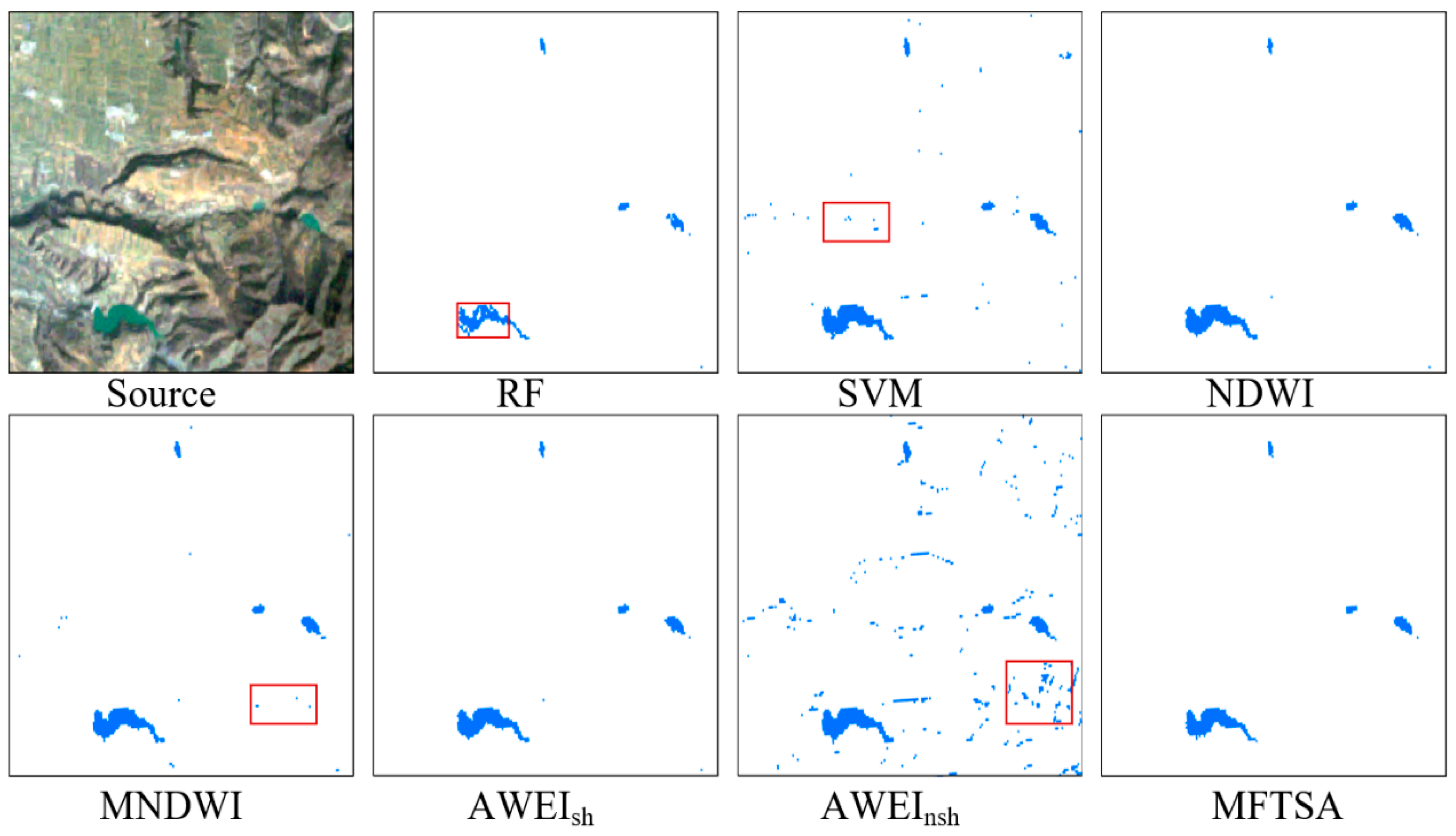
Three typical study areas including small water bodies were selected for comparative analysis on the classification results of machine learning. The extraction results of the three typical study areas are shown in Figure 9.
Study area (a) was a small ditch. The ditch was very narrow, occupying only about one or two pixels on the image. Before the addition of exponential features, RF mistakenly extracted many non-water pixels. After the addition of exponential features, the mistakenly extracted non-water pixels decreased, and the addition of exponential features could significantly improve the accuracy of small water bodies’ extraction (Figure 9). The water pixels were relatively continuous in the results of SVM extraction, but there were many wrongly extracted pixels beside the ditch. The water body was discontinuous in the results of RF extraction, and a lot of water pixels were missed. Adding remote-sensing index features greatly improved the accuracy of RF extraction ditches but had little effect on SVM extraction of water. The water bodies in (b) and (c) were aquaculture water and pond water. For aquaculture water and pond water, SVM extraction results showed that the water bodies were relatively complete, with clear boundaries, but the rate of false extraction was high. The main reason was that SVM recognized the soil pixel with high humidity as the water pixel. On the whole, the integrity of water extracted by SVM was better, but the false extraction rate was higher. The integrity of water extracted by RF was not as good as that of SVM, but the correct rate of extraction results was higher, which was consistent with the higher OA of RF in the test dataset and the lower SWER. The results and accuracy of different methods in the test dataset are shown in Table 5 and Table 6.
The OA index of the RF model was 1.02% higher than that of the SVM model. For the SWER index, the RF model was 4.9% lower than the SVM model. The main reason was that RF had a poor effect on small water bodies’ extraction for water boundary confusion pixels. The integrity of small water bodies extracted by SVM was relatively good, but many building shadows, mountain shadows and pond straws were extracted incorrectly. After adding index features, the UA of SVM decreased by 1.64%, the SWER of RF decreased by 2.15%, and all other indicators improved. The reason was that the added index feature was more capable of distinguishing vegetation and water bodies than the original feature dataset, but the ability to distinguish other categories was not as good as the original band, and the remote-sensing index features interfered with the classification.
4.3. Verification of Extraction Results by Different Methods
Due to the abnormal value of the image pixels, the water body extraction result inevitably has a small range of noise. Therefore, it was necessary to further process the extraction results to get the final result. Firstly, the water extraction results were converted from the raster format to the vector format, and then the Aggregate Polygon operation was carried out in ArcgisPro2.5. The reason for executing the Aggregate Polygon operation was that in the conversion process of water extraction results, some water bodies were divided into several small water bodies, which needed to be aggregated into one water element. We set the Aggregation Distance to 60 m, and then multiple water elements with a distance of less than 60 m were aggregated into one water element. Due to the limitation of image resolution, it was difficult to identify particularly small water bodies (<100 m2), so these water bodies were not included in the statistics. In the aggregation operation, Min Area and Min Hole Size were set to 100 m2, bodies of water less than 100 m2 in area were removed, and holes less than 100 m2 between vector bodies of water were filled as bodies of water. In order to compare the effects of different methods for extracting small water bodies, four regions (small rivers, aquaculture water, small urban reservoirs and small ponds in mountainous areas) were selected for comparative analysis.
Because of image resolution limitations, small rivers show small and narrow spatial characteristics on the image. Mixed pixels interfere with the extraction process of small rivers, resulting in discontinuity of the extracted river water. As shown in Figure 10, the RF method was not as good as the SVM method for the classification of mixed pixels, and the water body was missing in the red frame, while the SVM extraction result was relatively complete. The method misidentified many non-water bodies pixels, and the main ones were terrain shadows. had good results in removing topographic factors, but the identification of water bodies was incomplete. The main reason is that the method can remove shadows, which is suitable for areas where shadows are the main noise, and method can effectively eliminate non-water pixels on dark building surfaces and is suitable for scenes where shadows are not the main noise [15]. The water body information extracted by MNDWI is also mixed with a lot of shadow noise.
The area of aquaculture water is small, and its shape is generally rectangular. The nutrient level of aquaculture water has a certain impact on the spectral characteristics of a water body. There are generally pond ridges between different aquaculture water surfaces. The SVM method was not complete in extracting water bodies. The main missing locations were mostly located at the edge of the pond, which were mainly mixed pixels of water and non-water bodies (Figure 11). The water body extracted by SVM was complete, but the error rate of extraction rate was high. Not only the ridge of the pond but also the road next to the pond (inside the red frame) was identified as a body of water. In the red box of MNDWI extraction results, there were two slender aquaculture ponds with a pond boundary between the ponds. The MNDWI method identified the pond boundary as a water body and two small ponds as large ponds. In the red box, the body of water in the pond was not visible. In the identification of water bodies, some pond ridges were identified as water bodies, and the boundary between ponds was blurred. In contrast, the NDWI method and the MFTSA method had no missing extraction, and the water surface boundaries of different ponds were clear.
In urban areas, artificial building information is the dominant background information. The reflection of buildings is strong, while the reflection of water bodies is weak (Figure 12). Therefore, large background buildings and building shadows strongly interfere with water body extraction. The SVM method extracts water bodies incompletely. SVM seldom misses water bodies’ pixels in other scenes, but it misses water bodies in small urban reservoirs. The main reason is that small water bodies in cities appear black, and the spectral characteristics of water bodies in other places are not consistent. NDWI, MNDWI, and are relatively complete in extracting water bodies, but there are varying degrees of false extractions. Therefore, the RF and MFTSA methods are better in the identification of small urban water bodies.
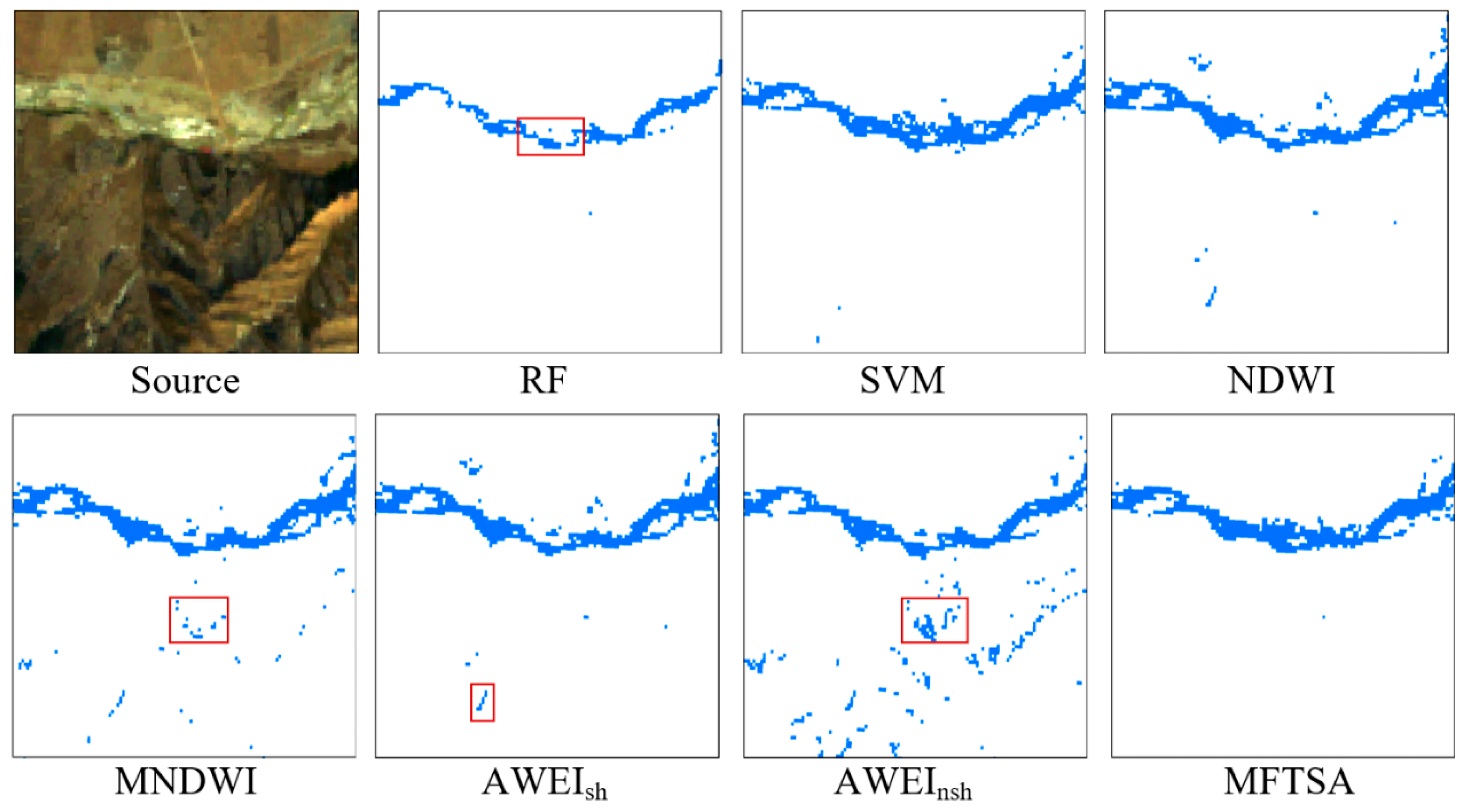
There are hill shadows between mountains. Although we used slope information to remove the hill shadows, it could only remove the hill shadows on the larger slopes. In some mountainous areas with smaller slopes, the effect of removing hill shadows was not good enough. As shown in Figure 13, the extraction results of the RF method leaked a part of the water body in the red frame, resulting in holes in the pond; SVM, MNDWI and recognized some mountain shadows as water bodies, and had the most serious misrecognition phenomenon, mainly because the index was suited for scenes without shadows. eliminates shadow pixels that are easy to confuse with water bodies in the result of , so the effect of extracting water bodies is better. On the whole, the NDWI, and MFTSA methods were better in extracting small water bodies in mountainous areas.
4.4. Spatial Distribution of Small Water Bodies on the Loess Plateau and Overall Accuracy Analysis
4.4.1. Spatial Distribution of Small Water Bodies on the Loess Plateau
The MFTSA method extracted a total of 71,592 water bodies on the Loess Plateau, with an area of 2921 km2 (Figure 14). The water bodies were mainly the Yellow River and other rivers, and the small water bodies were mainly distributed near the rivers and human living environments on the Loess Plateau.
4.4.2. Overall Accuracy Analysis of Small Water Bodies’ Extraction in Loess Plateau
Water bodies that are easily misidentified as non-water bodies include water bodies with large amounts of mud and sand, small ditches and some ponds on the Loess Plateau. The Yellow River has a high sediment content, and sediment accumulation occurs in some rivers. The spectral reflectance of water body pixels was weakened, and it was easy to miss the extraction and make the river interrupted in the extraction results.
Among all the methods, the RF, NDWI and methods had more serious leakages of small water bodies. The main objects of misidentification of small water bodies included terrain shadows, building shadows, dark impermeable surfaces and pond boundaries. Among all methods, the SVM, NDWI, MNDWI and methods had more misidentifications. The MFTSA method was better in removing mountain shadow and urban shadow noise while ensuring the integrity of water bodies, and the boundary of the extracted water body was clear. Statistics on water body results of the Loess Plateau extracted by the MFTSA are shown in Table 7.
The number of small water bodies in the Loess Plateau is 69,900, accounting for 97.63% of the total number of water bodies, but the area of small water bodies is small, accounting for only 16.50% of the total water body area. Among the three grades of small water bodies, the number of water bodies with an area range of 0.001–0.01 km2 accounts for 86.05% of the total small water bodies, and its area accounts for 45.02% of the total small water bodies. The water area in 0.001–0.01 km2 is mainly reservoirs, aquaculture and small puddles formed after the river stopped flowing.
5. Discussion
The new water extraction method developed in this paper is helpful to improve the accuracy of surface small water bodies’ mapping. However, the MFTSA method also has some limitations. For example, excessive nutrition of water bodies in aquaculture ponds or partial artificial facilities in ponds leads to spectral abnormalities of water bodies. For such water bodies, the extraction accuracy of MFTSA was poor, and some water pixels were not correctly extracted (Figure 11).
The Loess Plateau is mountainous, and the terrain is undulating. The use of remote-sensing methods is significantly affected by the terrain. Shadows restrict the accuracy of remote-sensing extraction of surface parameters. However, the MFTSA method can inhibit the mountain shadow and snow to a certain extent but cannot eliminate it. In the results of water extraction, there are still cases of misidentifying mountain shadows and snow as water bodies. It is difficult for different water index methods to eliminate the influence of mountain shadows and snow [10,19].
In addition, the selection of the threshold value of MFTSA methods is closely related to the land cover types, so the MFTSA methods are only applicable to the extraction of fine water bodies on the Loess Plateau, and the effect of extraction of small water bodies in other places may not be good. AWEI methods can be applied to surface water mapping in various environments [15]. Using deep learning to extract water can solve the problem of limited application scenarios of the model. Deep learning uses information fusion technology and a variety of networks to construct a water extraction model [27]. The deep learning method has a large demand for samples and a high requirement for sample quality. It takes a lot of time to make small-water-sample datasets. Moreover, the deep learning training model takes a long time and has high requirements for computer hardware [28]. Therefore, deep learning is suitable for extracting water in a small range from high-resolution remote-sensing images. The MFTSA method has small sample requirements, simple calculations and easy implementation, and is suitable for large-scale extraction of small water bodies.
6. Conclusions
This study takes the Loess Plateau with complex terrain as the research area and develops a multi-index fusion threshold segmentation algorithm (MFTSA) for a large-scale small water body extraction algorithm based on GEE (Google Earth Engine). The MFTSA uses AWEI, MNDWI, NDVI and EVI for multi-index synergy to extract small water bodies. It also uses NIR band reflectance and slope data generated by the SRTM digital elevation model to eliminate suppressing high-reflectivity noise and shadow noise. An MFTSA algorithm was developed and the results showed that:
- (1)
- It had high accuracy: the overall accuracy was 98.14% in the Loess Plateau, and the ratio of correctly extracted small water bodies was 92.82%.
- (2)
- Compared with traditional water index methods and the classification method, the MFTSA algorithm could extract small water with higher integrity and clearer and more accurate boundaries.
- (3)
- The MFTSA algorithm was used to extract a total of 69,900 small water bodies in the Loess Plateau, accounting for 97.63% of the total water bodies, and the area was 482.11 km2, accounting for 16.50% of the total water bodies.
The MFTSA method can be used to reflect the location and area information of small water bodies in the Loess Plateau, monitor the change characteristics of small water bodies, and reveal the temporal and spatial evolution of water bodies in the Loess Plateau. The MFTSA method can provide scientific reference for the ecological protection of the Loess Plateau and the sustainable utilization of regional water resources.
Author Contributions
Conceptualization: X.W. and C.W.; writing—original draft: J.G. and Y.Z.; writing—review and editing: X.W., C.W., J.G., B.L. and K.L. All authors have read and agreed to the published version of the manuscript.
Funding
This study was funded by the National Key Research and Development Program of China (2022YFF1300801) and the National Natural Science Foundation of China (U2243240, 42207396).
Data Availability Statement
This work also used the Landsat TM data acquired by the https://www.usgs.gov/ (accessed on 6 January 2023).
Acknowledgments
We gratefully acknowledged constructive suggestions by two anonymous reviewers and the editor, which helped improve the quality of manuscript greatly.
Conflicts of Interest
The authors declare no conflict of interest.
References
- Biggs, J.; von Fumetti, S.; Kelly-Quinn, M. The importance of small waterbodies for biodiversity and ecosystem services: Implications for policy makers. Hydrobiology 2017, 793, 3–39. [Google Scholar] [CrossRef]
- Golden, H.E.; Rajib, A.; Lane, C.R.; Christensen, J.R.; Wu, Q.S.; Mengistu, S. Non-floodplain wetlands affect watershed nutrient dynamics: A critical review. Environ. Sci. Technol. 2019, 53, 7203–7214. [Google Scholar] [CrossRef] [PubMed]
- Jiang, H.; Feng, M.; Zhu, Y.Q.; Lu, N.; Huang, J.X.; Xiao, T. An automated method for Extracting Rivers and Lakes from Landsat Imagery. Remote Sens. 2014, 6, 5067–5089. [Google Scholar] [CrossRef] [Green Version]
- Ji, L.; Zhang, L.; Wylie, B. Analysis of dynamic thresholds for the normalized difference water index. Photogramm. Eng. Remote Sens. 2009, 75, 1307–1317. [Google Scholar] [CrossRef]
- Jain, S.K.; Singh, R.D.; Jain, M.K.; Lohani, A.K. Delineation of flood-prone areas using remote sensing techniques. Water Resour. Manag. 2005, 19, 333–347. [Google Scholar] [CrossRef]
- Fisher, A.; Flood, N.; Danaher, T. Comparing Landsat water index methods for automated water classification in eastern Australia. Remote Sens. Environ. 2016, 175, 167–182. [Google Scholar] [CrossRef]
- Huete, A.; Didan, K.; Miura, T.; Rodriguez, E.P.; Gao, X.; Ferreira, L.G. Overview of the radiometric and biophysical performance of the MODIS vegetation indices. Remote Sens. Environ. 2002, 83, 195–213. [Google Scholar] [CrossRef]
- Aung, E.M.M.; Tint, T. Ayeyarwady river regions detection and extraction system from Google Earth imagery. In Proceedings of the 2018 IEEE International Conference on Information Communication and Signal Processing (ICICSP), Singapore, 28–30 September 2018; pp. 74–78. [Google Scholar]
- Liu, Q.H.; Huang, C.; Shi, Z.L.; Zhang, S.Q. Probabilistic river water mapping from Landsat-8 using the support vector machine method. Remote Sens. 2020, 12, 1374. [Google Scholar] [CrossRef]
- Yang, J.; Huang, X. The 30 m annual land cover dataset and its dynamics in China from 1990 to 2019. Earth Syst. Sci. Data 2021, 13, 3907–3925. [Google Scholar] [CrossRef]
- Farr, T.G.; Rosen, P.A.; Caro, E.; Crippen, R.; Duren, R.; Hensley, S.; Kobrick, M.; Paller, M.; Rodriguez, E.; Roth, L.; et al. The shuttle radar topography mission. Rev. Geophys. 2007, 45, RG2004. [Google Scholar] [CrossRef] [Green Version]
- Li, Y.; Niu, Z.G.; Xu, Z.Y.; Yan, X. Construction of high spatial-temporal water body dataset in China based on Sentinel-1 archives and GEE. Remote Sens. 2020, 12, 2413. [Google Scholar] [CrossRef]
- McFeeters, S.K. The use of the normalized difference water index (NDWI) in the delineation of open water features. Inter. J. Remote Sens. 1996, 17, 1425–1432. [Google Scholar] [CrossRef]
- Xu, H.Q. Modification of normalised difference water index (NDWI) to enhance open water features in remotely sensed imagery. Inter. J. Remote Sens. 2006, 27, 3025–3033. [Google Scholar] [CrossRef]
- Feyisa, G.L.; Meilby, H.; Fensholt, R.; Proud, S.R. Automated water extraction index: A new technique for surface water mapping using Landsat imagery. Remote Sens. Environ. 2014, 140, 23–35. [Google Scholar] [CrossRef]
- Otsu, N. A threshold selection method from gray-level histograms. IEEE Trans. Syst. Man Cybern. 1979, 9, 62–66. [Google Scholar] [CrossRef] [Green Version]
- Dong, J.W.; Xiao, X.M.; Kou, W.L.; Qin, Y.W.; Zhang, G.L.; Li, L.; Jin, C.; Zhou, Y.T.; Wang, J.; Biradar, C.; et al. Tracking the dynamics of paddy rice planting area in 1986-2010 through time series Landsat images and phenology-based algorithms. Remote Sens. Environ. 2015, 160, 99–113. [Google Scholar] [CrossRef]
- Rouse, J.W., Jr.; Haas, R.H.; Schell, J.A.; Deering, D.W. Third Earth Resources Technology Satellite-1 Symposium: The Proceedings of a Symposium Held by Goddard Space Flight Center at Washington, DC on 10–14 December 1973: Prepared at Goddard Space Flight Center; Scientific and Technical Information Office, National Aeronautics and Space Administration: Washington, DC, USA, 1974; Volume 351, p. 309. [Google Scholar]
- Deng, Y.; Jiang, W.G.; Tang, Z.H.; Ling, Z.Y.; Wu, Z.F. Long-Term Changes of Open-Surface Water Bodies in the Yangtze River Basin Based on the Google Earth Engine Cloud Platform. Remote Sens. 2019, 11, 2213. [Google Scholar] [CrossRef] [Green Version]
- Sarp, G.; Ozcelik, M. Water body extraction and change detection using time series: A case study of Lake Burdur, Turkey. J. Taibah Univ. Sci. 2017, 11, 381–391. [Google Scholar] [CrossRef] [Green Version]
- Breiman, L. Random forests. Mach. Learn. 2001, 45, 5–32. [Google Scholar] [CrossRef] [Green Version]
- Belgiu, M.; Dragut, L. Random forest in remote sensing: A review of applications and future directions. ISPRS J. Photogram. Remote Sens. 2016, 114, 24–31. [Google Scholar] [CrossRef]
- Corcoran, J.M.; Knight, J.F.; Gallant, A.L. Influence of multi-source and multi-temporal remotely sensed and ancillary data on the accuracy of random forest classification of Wetlands in Northern Minnesota. Remote Sens. 2013, 5, 3212–3238. [Google Scholar] [CrossRef] [Green Version]
- Zhou, L.; Luo, T.; Du, M.; Qiang, C.; Yang, L.; Yinuo, Z.; Congcong, H.; Siyu, W.; Kun, Y. Machine learning comparison and parameter setting methods for the detection of dump sites for construction and demolition waste using the google earth engine. Remote Sens. 2021, 13, 787. [Google Scholar] [CrossRef]
- Cortes, C.; Vapnik, V. Support-vector networks. Mach. Learn. 1995, 20, 273–297. [Google Scholar] [CrossRef]
- Zou, Z.H.; Xiao, X.M.; Dong, J.W.; Qin, Y.W.; Doughty, R.B.; Menarguez, M.A.; Zhang, G.L.; Wang, J. Divergent trends of open-surface water body area in the contiguous United States from 1984 to 2016. Proc. Natl. Acad. Sci. USA 2018, 115, 3810–3815. [Google Scholar] [CrossRef] [Green Version]
- Chen, Y.; Fan, R.S.; Yang, X.C.; Wang, J.X.; Latif, A. Extraction of Urban Water Bodies from High-Resolution Remote-Sensing Imagery Using Deep Learning. Water 2018, 10, 585. [Google Scholar] [CrossRef] [Green Version]
- Li, Y.S.; Dang, B.; Zhang, Y.J.; Du, Z.H. Water body classification from high-resolution optical remote sensing imagery: Achievements and perspectives. ISPRS J. Photogramm. Remote Sens. 2022, 187, 306–327. [Google Scholar] [CrossRef]
Figure 1.
The study area.

Figure 2.
Technical flow chart. RF, random forest; SVM, support vector machine; CLCD, China Land Cover Dataset; NDWI, normalized difference water index; MNDWI, modified normalized difference water index; , automated water extraction index with shadows elimination; , automated water extraction index with no shadows elimination.

Figure 3.
Density maps of water and others objects with different water body indices.

Figure 4.
The scatter density of training samples. (a,b) Water samples; (c,d) non-water samples.

Figure 5.
Differences in AWEIsh and AWEInsh of land cover types.

Figure 6.
The comparison of results of different water extraction algorithms. (a) Ditch study area; (b,c) pond study areas.
Figure 6.
The comparison of results of different water extraction algorithms. (a) Ditch study area; (b,c) pond study areas.

Figure 7.
Accuracy of RF and SVM for extracted small water bodies.

Figure 8.
The importance of individual independent variables in the RF model.

Figure 9.
Comparison of water extraction results by different classification methods. (a) Ditch study area; (b,c) study areas for aquaculture water bodies and pond water bodies.
Figure 9.
Comparison of water extraction results by different classification methods. (a) Ditch study area; (b,c) study areas for aquaculture water bodies and pond water bodies.

Figure 10.
Comparison of extraction results by different methods in small river study area (The red box shows where the extraction went wrong).
Figure 10.
Comparison of extraction results by different methods in small river study area (The red box shows where the extraction went wrong).

Figure 11.
Comparison of extraction results of different methods in aquaculture water area (The red box shows where the extraction went wrong).
Figure 11.
Comparison of extraction results of different methods in aquaculture water area (The red box shows where the extraction went wrong).

Figure 12.
Comparison of extraction results of different methods in a small urban reservoir (The red box shows where the extraction went wrong).
Figure 12.
Comparison of extraction results of different methods in a small urban reservoir (The red box shows where the extraction went wrong).

Figure 13.
Comparison of extraction results of different methods for small mountain pond (The red box shows where the extraction went wrong).
Figure 13.
Comparison of extraction results of different methods for small mountain pond (The red box shows where the extraction went wrong).

Figure 14.
Water bodies’ extraction results of method based on the MFTSA on the Loess Plateau.


Table 1.
Calculation formula of remote-sensing feature indices.
| Name of Index | Formula |
|---|---|
| NDVI | |
| EVI | |
| NDWI | |
| MNDWI | |
| AWEI |
Note: Blue, Green, Red, NIR, SWIR1 and SWIR2 are the blue band, green band, red band, near-red band, SWIR1 band and SWIR2 band of Landsat5, respectively.
Table 2.
Landsat5 band information. The source of band information is: https://www.usgs.gov/landsat-missions/landsat-5 (accessed on 6 January 2023).
Table 2.
Landsat5 band information. The source of band information is: https://www.usgs.gov/landsat-missions/landsat-5 (accessed on 6 January 2023).
| Band Index | Band Name | Wavelength (µm) | Resolution (m) |
|---|---|---|---|
| Band-1 | Blue | 0.45–0.52 | 30 |
| Band-2 | Green | 0.52–0.60 | 30 |
| Band-3 | Red | 0.63–0.69 | 30 |
| Band-4 | NIR | 0.76–0.90 | 30 |
| Band-5 | SWIR1 | 1.55–1.75 | 30 |
| Band-6 | LWIR | 10.40–12.50 | 120 |
| Band-7 | SWIR2 | 2.08–2.35 | 30 |
Table 3.
Analysis of different threshold segmentation methods’ results.
| Classes\Methods | All | NDWI | MNDWI | MFTSA | ||
|---|---|---|---|---|---|---|
| River | 831 | 595 | 869 | 868 | 844 | 862 |
| Lakes | 557 | 502 | 551 | 541 | 521 | 549 |
| Reservoir | 790 | 699 | 763 | 755 | 686 | 762 |
| Small water | 836 | 573 | 773 | 737 | 537 | 776 |
| Shadow | 1306 | 1293 | 1280 | 1254 | 1294 | 1292 |
| Snow | 865 | 878 | 857 | 882 | 887 | 877 |
Table 4.
Analysis of different threshold segmentation methods’ accuracy.
| Methods\Accuracy | PA (%) | UA (%) | OA (%) | Kappa | SWER (%) |
|---|---|---|---|---|---|
| NDWI | 78.60 | 98.75 | 87.06 | 0.74 | 68.54 |
| MNDWI | 98.08 | 97.88 | 97.66 | 0.95 | 92.46 |
| 96.25 | 97.81 | 96.59 | 0.93 | 88.16 | |
| 85.87 | 99.23 | 91.45 | 0.83 | 64.23 | |
| MFTSA | 97.84 | 98.93 | 98.14 | 0.96 | 92.82 |
Table 5.
The extraction results of different classification methods.
| Classes\Methods | All | SVM_NoVI | SVM | RF_NoVI | RF |
|---|---|---|---|---|---|
| River | 831 | 796 | 799 | 805 | 806 |
| Lakes | 557 | 522 | 535 | 544 | 550 |
| Reservoir | 790 | 676 | 727 | 729 | 745 |
| Small water | 836 | 755 | 759 | 736 | 718 |
| Shadow | 1306 | 1201 | 1135 | 1154 | 1196 |
| Snow | 865 | 880 | 884 | 885 | 877 |
Table 6.
Extraction accuracy analysis of different classification methods.
| Methods\Accuracy | PA (%) | UA (%) | OA (%) | Kappa | SWER (%) |
|---|---|---|---|---|---|
| SVM_NoVI | 91.21 | 95.82 | 92.62 | 0.85 | 90.31 |
| SVM | 93.56 | 93.94 | 92.79 | 0.85 | 90.79 |
| RF_NoVI | 93.36 | 94.56 | 93.06 | 0.86 | 88.04 |
| RF | 93.53 | 95.66 | 93.81 | 0.87 | 85.89 |
Table 7.
Statistics of MFTSA water extraction results.
| Type of Water Body | Class of Area (km2) | Number | Area (km2) |
|---|---|---|---|
| Small water | 0.001~0.01 | 60,152 | 217.06 |
| 0.01~0.05 | 8483 | 176.49 | |
| 0.05~0.1 | 1265 | 88.56 | |
| Others | >0.1 | 1692 | 2439.12 |
| Total | 71,592 | 2921.23 |
Disclaimer/Publisher’s Note: The statements, opinions and data contained in all publications are solely those of the individual author(s) and contributor(s) and not of MDPI and/or the editor(s). MDPI and/or the editor(s) disclaim responsibility for any injury to people or property resulting from any ideas, methods, instructions or products referred to in the content. |
© 2023 by the authors. Licensee MDPI, Basel, Switzerland. This article is an open access article distributed under the terms and conditions of the Creative Commons Attribution (CC BY) license (https://creativecommons.org/licenses/by/4.0/).
Share and Cite
MDPI and ACS Style
Guo, J.; Wang, X.; Liu, B.; Liu, K.; Zhang, Y.; Wang, C. Remote-Sensing Extraction of Small Water Bodies on the Loess Plateau. Water 2023, 15, 866. https://doi.org/10.3390/w15050866
AMA Style
Guo J, Wang X, Liu B, Liu K, Zhang Y, Wang C. Remote-Sensing Extraction of Small Water Bodies on the Loess Plateau. Water. 2023; 15(5):866. https://doi.org/10.3390/w15050866
Chicago/Turabian StyleGuo, Jia, Xiaoping Wang, Bin Liu, Ke Liu, Yong Zhang, and Chenfeng Wang. 2023. "Remote-Sensing Extraction of Small Water Bodies on the Loess Plateau" Water 15, no. 5: 866. https://doi.org/10.3390/w15050866
Note that from the first issue of 2016, this journal uses article numbers instead of page numbers. See further details here.