Atmospheric Exchange of Carbon Dioxide and Water Vapor above a Tropical Sandy Coastal Plain

Abstract

As a unique type of ecosystem, tropical coastal sandy vegetation lies in the transition zone extending from coastal beaches to further inland and provides important ecosystem services such as windproofing, tourism, and agriculture. However, the energy and matter fluxes of these tropical coastal ecosystems have been rarely studied. We reported one-year eddy flux observations in a tropical sandy coastal ecosystem and specifically focused on the carbon and water exchanges between the atmosphere and the ecosystem. The studied ecosystem was a carbon sink (approximately –560 gC m⁻² yr⁻¹) and approximately 1000 mm of water evaporated from the ecosystem into the atmosphere during the study year. The highest levels of vegetation photosynthesis occurred in April, shortly before the wet season. This can be attributed to an endogenous self-adjustment of the ecosystem to improve the water- and carbon-use efficiency during the wet season. This study is expected to not only fill the data gap with respect to the gas exchange between tropical sandy coastal plains and the atmosphere but also provide knowledge about the function and ecological service of these specific ecosystems.

1. Introduction

The measurement of ecosystem carbon flux has important ecological significance in the study of the global carbon cycle and exploring the response of carbon sources/sinks in different ecosystems has become one of the key issues in ecological research [1,2]. The eddy covariance (EC) technique is a widely used method to explore the energy and material cycle in the soil–vegetation–atmosphere interface; it can directly measure the physical characteristics of ecosystems because of its effectiveness and feasibility in continuous monitoring of carbon flux and meteorological factors [3,4,5,6]. There have been numerous works of research conducted using the EC technique to investigate the variation of ecosystem carbon fluxes temporally and its controlling factors. For example, after analyzing multi-year carbon flux observation data from 59 observation stations around the world, Baldocchi et al. [7] preliminarily answered the question of how ecosystems control the changes in ecosystem carbon flux through different climatic factors and ecological environments, and analyzed different inter-annual variations of ecosystem carbon flux. Across the boreal forests, the inter-annual standard deviation of net carbon fluxes was relatively small [8,9,10,11,12]. Year-to-year changes in net carbon exchange were attributed to changes in air temperature, soil moisture, water balance, and summer solar radiation [13,14]. Temperate evergreen forests cover a wide range of climatic and soil conditions and are often intensively managed [15]. Long-term carbon fluxes often include additional changes due to disturbances [16,17]. Light and temperature were the main meteorological factors responsible for the inter-annual variation in carbon fluxes, the study reported [18,19,20,21,22].

Countries and regions such as the United States and Europe have initiated and established regional network systems since the 1960s [23,24] for long-term monitoring of atmospheric and flux changes in the community to investigate the balance mechanism of material and energy exchange in ecosystems. At present, there are more than 900 flux observation stations worldwide [25]. Although the global flux monitoring system has been gradually improved, the distribution of sites is still relatively uneven, with more stations in high-latitude areas than in low-latitude areas. Specifically, there are very few reports on carbon flux changes in tropical sandy coastal ecosystems.

Sandy coastal ecosystems lie in the transition zone extending from coastal beaches to further inland, and sandy plains are formed by the weathering of coastal sediments. Their ecosystem structure is simple, the soil sand is loose, the water-holding capacity is poor, the nutrient content is extremely low, and the salinization degree is high [26]. Therefore, responses and feedback to environmental factors can be quickly determined. These unique ecosystems are important not only because they serve as a buffer for coastline safety but also because of their recreation, tourism, and agricultural roles. These ecosystems are especially important for islands, which usually have a long, mainly sandy, coastal line. Although sandy coastal ecosystems only account for 3% of the total area of Hainan Island, the unique geographical location and special carbon storage mechanism create an important role in the carbon cycle process in this region [27]. In the past decades, the Chinese government has invested large efforts to protect and recover the vegetation of sandy coastal plains. The major aim is to improve the ecological service of these ecosystems, such as through sand stabilization, avoiding soil salinization, and reducing destruction from typhoons.

Long-term ecological monitoring was carried out in a typical sandy coastal plain in Hainan in 2008. As a major part of these ecological observations, an eddy flux tower was established and related measurements started in 2015. In this study, we reported the eddy flux observation results. Our specific objectives were to: (i) quantify the magnitude and variation of carbon dioxide and water vapor fluxes between the studied ecosystem and the atmosphere after thorough data quality control and assessment, (ii) understand the carbon and water fluxes from a canopy conductance perspective, and (iii) provide possible explanations of the observed patterns and findings. The results can both provide information for the analysis of carbon flux changes in terrestrial ecosystems and improve our understanding of the function and ecological service of these specific ecosystems.

2. Materials and Methods

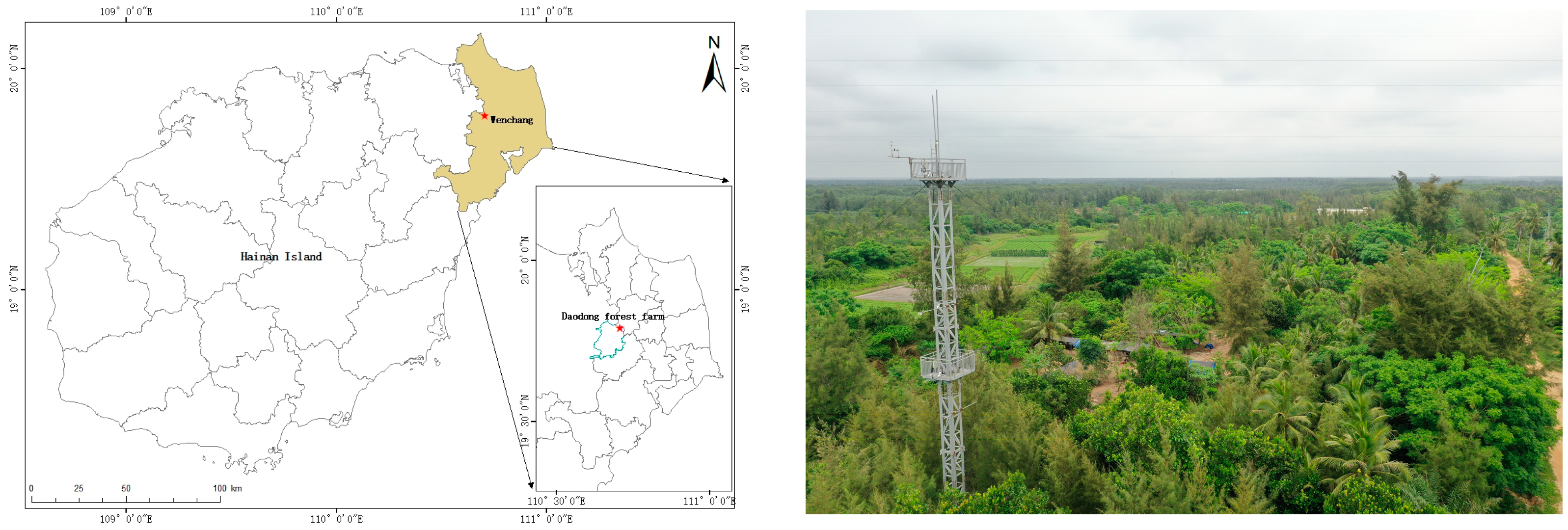
2.1. Site Description

The study site is located in Hainan Province, Southern China. The eddy flux tower is geographically located in the easternmost state forest farm of Hainan Island (19°44′ N 110°57′ E), which is close to the South China Sea in the Pacific Ocean (Figure 1). The sandy coastal plain terrain is flat. The mean elevation is ~62.9 m. This region is dominated by a tropical ocean monsoon climate, with a clearly divided dry and wet season. According to local climatic data, the period between May and October is categorized as the wet season. The multi-year mean rainfall is 1721 mm, and the annual precipitation recorded by the rain gauge at the top of the tower during the study period was 1482 mm, with over 80% of rainfall occurring in the wet season. The mean annual temperature is ~23.9 °C. Extreme low temperatures can be as low as ~10 °C. The pan evaporation is as high as 1900 mm. Tropical storms and typhoons occur in this region with a relative high frequency (2.6 times per year on average). The sandy soil developed from marine sediment caused by seawater encroachment in the Quaternary. The vegetation is a combination of planted trees and local native trees and can be categorized as an evergreen forest. The major planted trees include Casuarina equisetifolia, Cocos nucifera, Eucalyptus robusta, Acacia mangium, Acacia auriculiformis, Acacia crassicarpa, and Calophyllum inophyllum. The local native trees include Homalium hainanense, Dalbergia odorifera, and Ficus variegata. The dominant shrub species are Rhodomyrtus tomentosa, Atalantia buxifolia, Psychotria rubra, Cherodendrum cyrtophyllum, and Wikstroemia indica. Casuarina equisetifolia is the main tree species of the coastal shelterbelt and the canopy closure is 65% to 75%. Both shrubs and herbs grow well due to the open canopy. The main vegetation canopy height is ~7 m. The leaf area index is ~2.5 m² m⁻² in the wet season. Some of the taller trees fell in a strong “Rammasun typhoon” that occurred in 2014. The forest canopy is still not fully closed [28,29].

2.2. Instrumentation and Observations

The eddy flux tower has a height of 25 m and is square-shaped. A special design was implemented for the tower to protect it from typhoons. General information on instruments, manufacturers, and operation height is listed in

Table 1. Summary of instrumentation information.

Instruments	Model	Manufacturer	Height or Depth
Sonic anemometer	WindMaster	Gill Instruments, Lymington, UK	25 m
Infrared gas analyzer	Li-7500A	Li-Cor Inc., Lincoln, USA	25 m
Net radiometer	NR01	Hukseflux, Delft, Netherlands	12 m
Photosynthetically active radiation	Li-190SL	Li-Cor Inc., Lincoln, USA	24, 18, 13, 3 m
Wind cup	03001	RM Young, Traverse City, USA	24, 18, 13, 3 m
Humidity and temperature probe	HMP-60	Vaisala, Vantaa, Finland	24, 18, 13, 3 m
Rain gauge	TE-525	Texas Electronics, Dallas, USA	24, 2 m
Soil heat flux	HFP01	Hukseflux, Delft, Netherlands	−10 cm
Soil temperature	TM-L10	Dynamax Inc., Houston, USA	−10, −20, −40, −80 cm
Soil water content	EC-5	Decagon, Pullman, USA	−10, −20, −40, −80 cm
Flux-calculating module	SmartFlux	Li-Cor Inc., Lincoln, Nebraska USA	24 m

.

In general, the instruments on the tower can be categorized into two parts: eddy covariance and routine microenvironmental systems. The eddy covariance system comprises a three-dimensional sonic anemometer and an open-path infrared gas analyzer. They are controlled by a commercial interface (Li-7550) design by Li-Cor. The sampling frequency for both wind velocity and gas concentration is 10 Hz. The data were recorded using a 16 GB USB flash drive. The data were manually copied to the laboratory computer every three months. The net radiometer can measure global/reflected solar radiation and infrared radiation. The climatic factors were sampled every 10 s and a 10 min mean value was recorded by a data logger (CR1000, Campbell Scientific Inc., Logan, UT, USA).

Errors may be present as the instrument is easily affected by terrain factors, climatic factors, and the instrument itself. In order to reduce the interference of external factors on the results of the data, it was necessary to correct the original data. Therefore, the 3 components of the wind speed are rotated quadratics so that the average crosswind speed and the average vertical wind speed are 0.

2.3. Eddy Flux Calculation

Turbulence plays a major role in atmospheric boundary layer mass and energy transport. In the eddy covariance technique, the vertical transported entity at a point is calculated as the correlation between the fluctuations of the concentration of that entity and the fluctuations of the vertical wind speed [30]. The annual sum of evapotranspiration (E) is estimated from the latent heat flux (λE) divided by λ. Nevertheless, the negative E values occurred within this observational time series. We performed two types of treatment on these negative values. First, we treated the negative values as zero. Subsequently, the annual sum of E was estimated. Secondly, we treated negative values as data gaps. It is common that the energy balance is not closed in eddy covariance observations. This leads to the underestimation of E. We corrected this energy imbalance by assuming that the Bowen ratio (β) is reliable. Subsequently, the fluxes of carbon dioxide (F_c), latent heat (λE), evapotranspiration (E) and sensible heat (H) were calculated as:

$$\begin{gathered} {\mathrm{CO}}_2 \mathrm{flux}, F_{\mathrm{c}}=-\overline{w^{\prime }{c}^{\prime }} \\ \mathrm{Latent} \mathrm{heat} \mathrm{flux},\lambda E=-\lambda \overline{w^{\prime }{q}^{\prime }} \\ \mathrm{Evapotranspiration} \mathrm{flux}, E=\lambda E/\lambda =(Rn-G)(1/(\beta +1)) \\ \mathrm{Sensible} \mathrm{heat} \mathrm{flux},H=-\rho C_p\overline{w^{\prime }{T}^{\prime }} \end{gathered}$$

where w is the vertical velocity on rotated coordination, c is the CO₂ concentration, λ is the latent heat of vaporization, q is the absolute humidity, ρ is air density, C_p is the specific heat of the air at a constant pressure, and T is air temperature. The bar indicates the time averages and the prime denotes the deviation from those averages.

2.4. Processing of Eddy Flux Data

We used a commercial program (EddyPro^®,Li-Cor Inc., Lincoln, NE, USA) to process the raw 10 Hz data to obtain 30 min fluxes. The basic settings of EddyPro in our case include: (i) the double rotation method for tilt correction [31], (ii) the WPL method to correct for the air density effect [32], (iii) the block average method to accomplish detrending, (iv) the Kljun et al. [33] method to estimate the footprint, (v) spectral correction according to Moncrieff et al. [34], (vi) raw 10 Hz data screening according to Vickers and Mahrt [35], and (vii) the calculation of the storage flux to obtain the net ecosystem exchange (NEE).

We performed several quality assessment and control steps on the 30 min flux data: (i) we checked the energy balance closure with 30 min data and examined the effect of this energy imbalance on the water vapor flux estimation, (ii) we identified a threshold friction velocity (u*) for nighttime F_c underestimation according to Saleska et al. [36], (iii) we accomplished data gap filling using the mean diurnal variation method [37], and (iv) we performed light response analysis of the daytime carbon fluxes and temperature responses to nighttime carbon fluxes.

2.5. Calculations and Statistics

Based on Penman [38]’s big-leaf model, the biosphere–atmosphere exchange of H₂O can be expressed as:

$$\lambda E=g\left(\rho C_p/\gamma \right)\left(e_i-e_a\right)$$

where γ is the psychrometer constant, e_i is the water vapor pressure at the ecosystem’s surface, e_a is the water vapor pressure in the air at the reference height, and the term g is usually interpreted as:

$$1/g=1/g_s+1/g_a$$

where g_s is the surface conductance, which mainly describes the bulk stomatal conductance, and g_a is the aerodynamic conductance.

Because plant CO₂ assimilation and H₂O transpiration are two processes coupled through stoma, a better knowledge of g_s benefits our understanding of both H₂O and CO₂ exchanges. The g_s value is usually inferred by inverting the Penman–Monteith equation as:

$$\frac{1}{g_s}=\frac{\rho C_P}{\gamma }\frac{D}{\lambda E}+\left(\frac{\Delta }{\gamma }\beta -1\right)\left(\frac{1}{g_{\mathrm{a}}}\right)$$

where D is the air water vapor deficit, β is the Bowen ratio (H/λE), and Δ is the slope of the saturated vapor pressure vs. the temperature curve (∂e_s(T)/∂T). Verma [39]’s expression for g_a is used in this study as:

$$\frac{1}{g_a}=\frac{u}{u_{*}^2}+\frac{D}{\kappa u_{*}}\left(\ln \left(\frac{z_{OM}}{z_{OH}}\right)+{\Psi }_M-{\Psi }_H\right)$$

where u is the mean wind speed, u* is the friction velocity, κ is the Karman constant, Z_OM and Z_OH are roughness lengths for momentum and heat transfer, and Ψ_M and Ψ_H are the diabatic stability correction functions for momentum and heat, respectively. Paulson [40]’ s expression for Ψ_M and Ψ_H is:

$$\begin{gathered} {\Psi }_M=2{\displaystyle {\int }_0^x\left(\frac{1}{1+x\prime }+\frac{x\prime }{1+x{\prime }^2}\prime \frac{1}{1+x{\prime }^2}\right)dx\prime } \\ {\Psi }_M=2\ln [(1+x)/2]+\ln [(1+x^2)/2]-2{\tan }^{-1}x+\pi /2 \\ {\Psi }_H=2{\displaystyle {\int }_0^{x^2}{\frac{d(x{\prime }^2)}{1+x{\prime }^2}}^{\prime }} \\ {\Psi }_H=2\ln [(1+x^2)/2] \end{gathered}$$

where $x={(1-\gamma z/L)}^{1/4}$, z is the vertical space coordinate, and L is $-u_{*}^3{c}_p\rho T/(kgH)$.

The Michaelis–Menten model was used to fit the relationship between the net carbon dioxide flux of the ecosystem and the photosynthetically active radiation during the day [41]. The daytime NEE is defined as:

$$-NE{E}_{\mathrm{day}}=\frac{A_{\mathrm{QY}}{P}_{\max }PAR}{A_{\mathrm{QY}}PAR+P_{\max }}-R_{\mathrm{d}}$$

where A_QY is the apparent quantum yield, Pmax is the maximum light net photosynthetic rate, PAR is photosynthetically active radiation, and R_d is the dark respiration rate. The ecosystem only performs respiration at night, and temperature is an important factor controlling the respiration of the ecosystem. The relationship between temperature and the ecosystem can be determined by the van’t Hoff function [42]; the nighttime NEE is defined as:

$$NE{E}_{\mathrm{night}}=R_0{(Q_{10})}^{T_{\mathrm{a}}/10}$$

where R₀ is the ecosystem respiration at 0 °C, and Q₁₀^Ta/10 is the relative increase in respiration per 10 °C temperature increase.

The Jarvis Omega [43] and Priestley–Taylor Alpha [44] were also calculated as:

$$\Omega =\frac{\Delta /\gamma +1}{\Delta /\gamma +1+g_a/g_c}$$

$$\alpha =\lambda E/[(\lambda E+H)(\Delta /(\Delta +\gamma ))]$$

2.6. Net Photosynthetic Rate

The formula for calculating the net photosynthetic rate P_n is defined as:

$$P_n=\frac{A_{QY}I+P_{\max }-\sqrt{{\left(A_{QY}I+P_{\max }\right)}^2-4\theta A_{QY}I{P}_{\max }}}{2\theta }-R_d$$

where P_n is the net photosynthetic rate, A_QY is the apparent quantum yield, P_max is the maximum light net photosynthetic rate, R_d is the dark respiration rate, I is the radiation intensity, and θ is the curvature of the curve.

$$P_{\max }=A_{QY}\times I_{\mathrm{sat}}-R_{\mathrm{d}}$$

where I_sat is the light saturation point.

A glossary of terms mentioned above are listed in Table S1.

3. Results

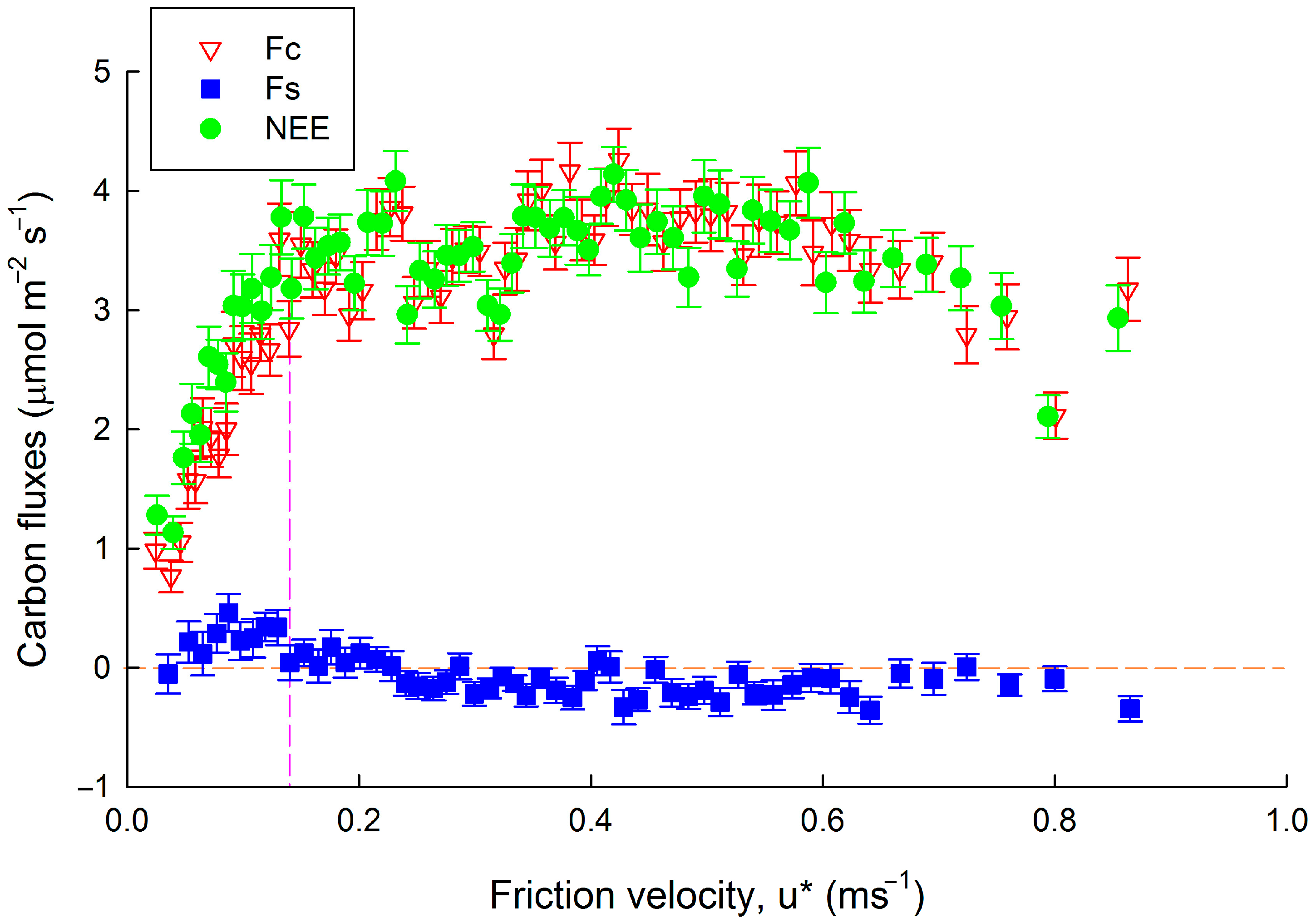
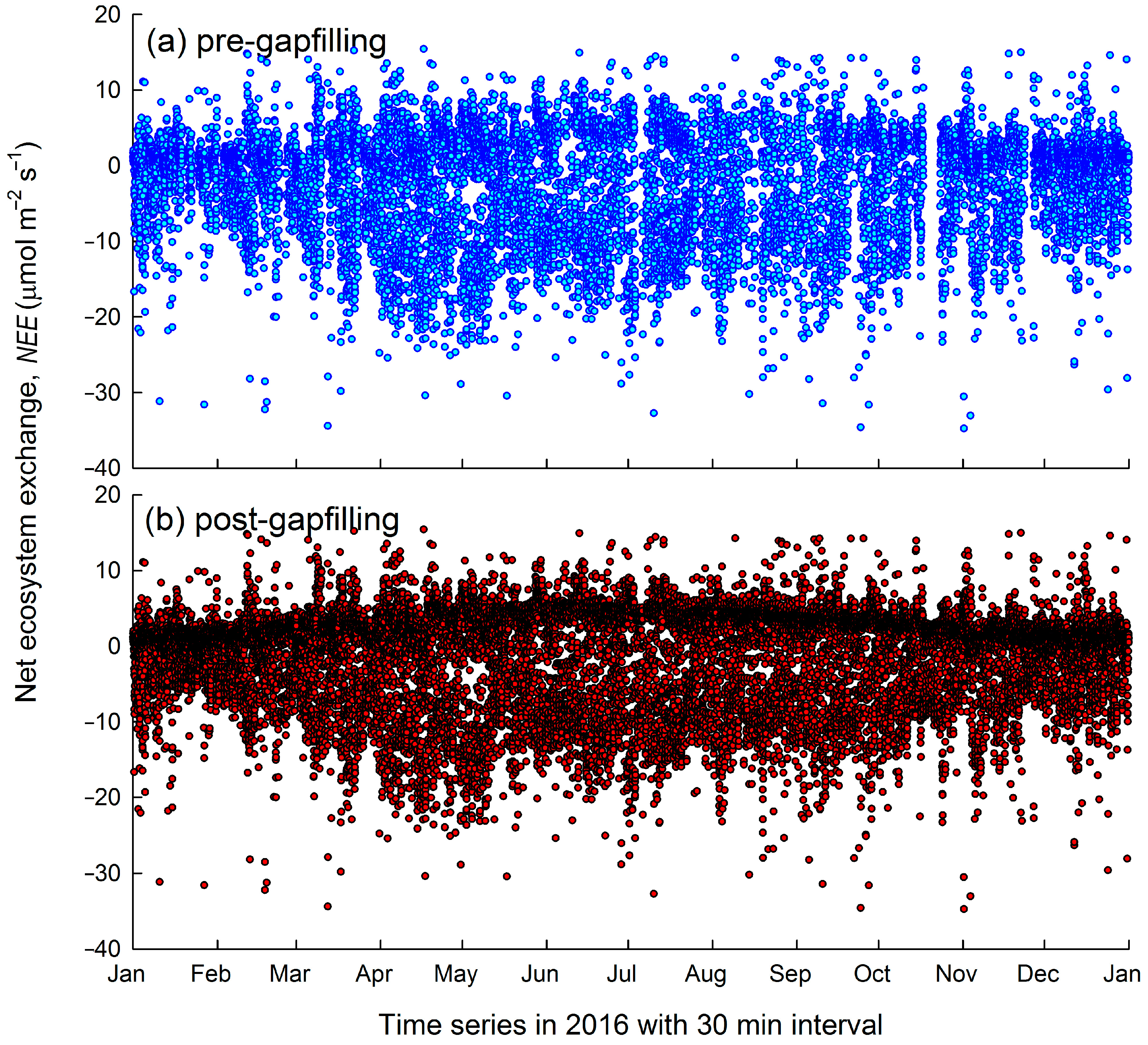
3.1. Nighttime Flux Underestimation

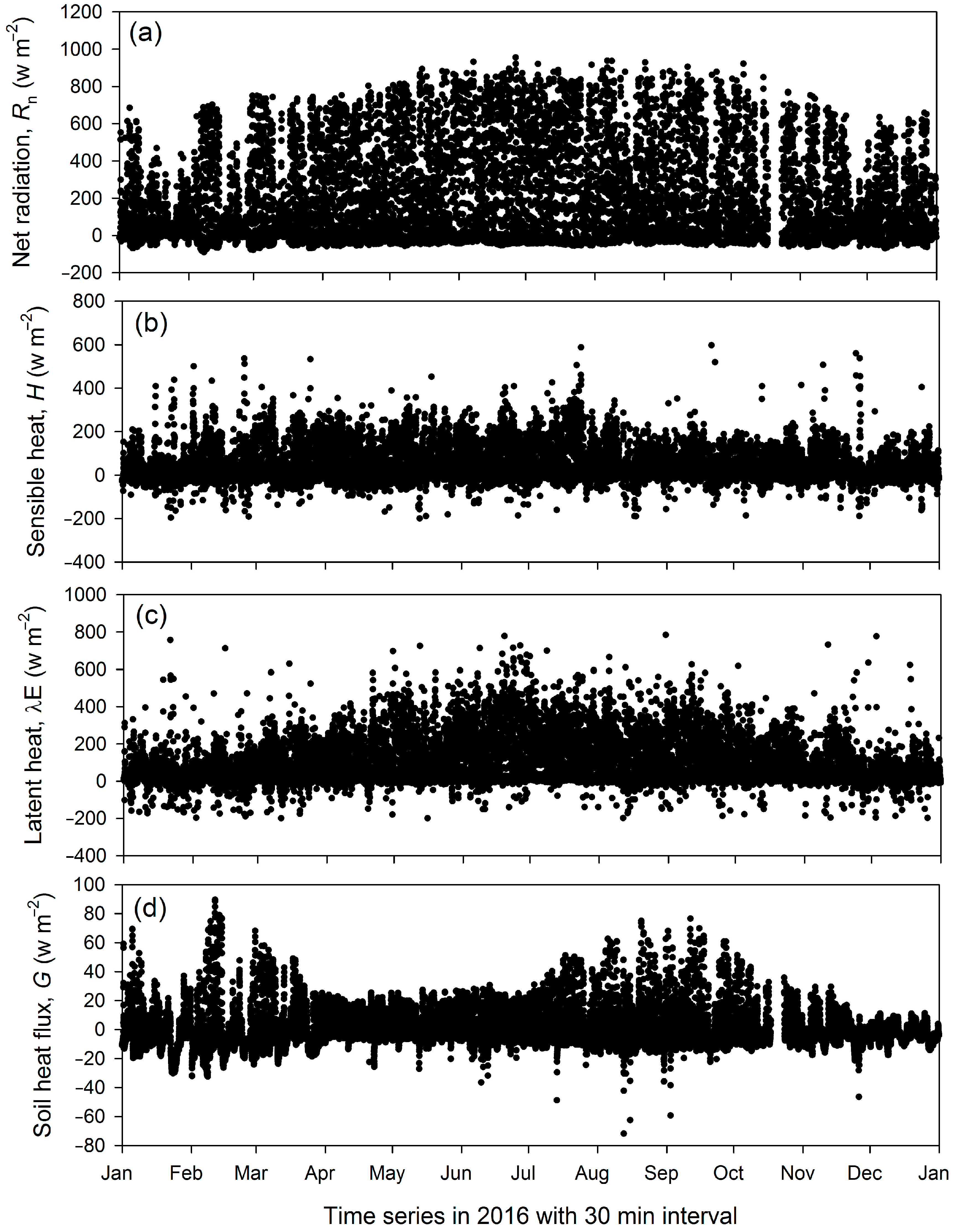
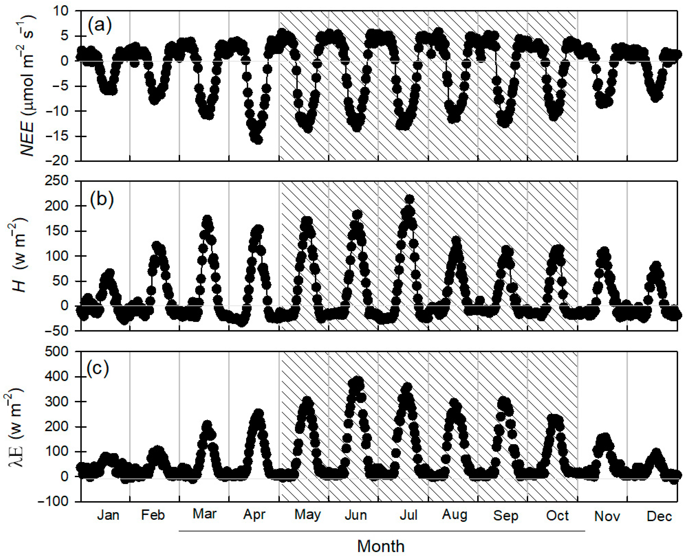
The changes in the carbon fluxes and the increasing friction velocity (u*) are shown in Figure 2. The main vegetation canopy height was ~7 m and the canopy was open. In this case, the storage flux (F_s) was very close to zero and played a negligible role in the net ecosystem exchange (NEE). Both the eddy-transported carbon flux (F_c) and NEE dramatically changed with u* at a low u* level when u* < 0.17 m s⁻¹. They showed some kind of saturation trend when u* was larger than 0.17 m s⁻¹. The threshold u* could easily be determined as 0.17 m s⁻¹.

3.2. Energy Fluxes

Four major ecosystem energy flux components are shown in Figure 3. The net radiation (R_n) was the major energy input of the studied ecosystem and drove other processes such as the evaporation of water, photosynthesis, and temperature changes. The daily peak R_n showed seasonal variations with a higher value in the wet season than in the dry season. The sensible heat flux (H) did not show a clear seasonal pattern compared with that of the latent heat flux (λE); λE was higher in the wet season than in the dry season. The soil heat flux (G) reached nearly 100 w m⁻² in some cases, which was comparable to the values of H and λE. This might be related to the open canopy, which led to a large proportion of solar radiation penetrating to the soil surface. The seasonal variation of precipitation (P) is shown in Figure 4.

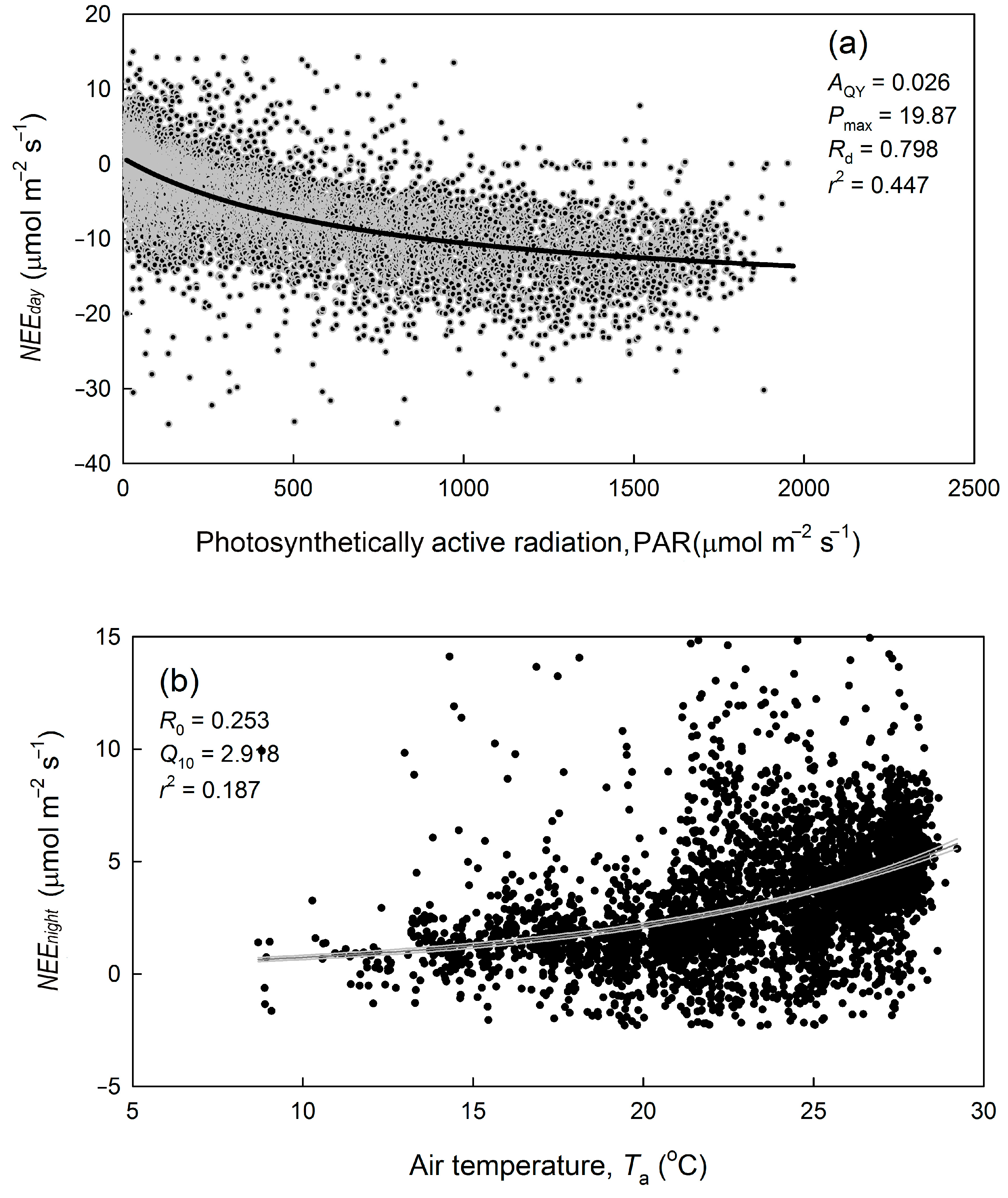
3.3. Carbon Dioxide Flux and Its Environmental Response

The daytime NEE was strongly dependent on photosynthetically active radiation (PAR; Figure 5). The PAR explained approximately 45% of the daytime NEE variance. The apparent quantum yield (A_QY) was 0.026 μmol m⁻² s⁻¹ C per μmol m⁻² s⁻¹ photons. The light-saturated photosynthesis rate (P_max) was ~19.87 μmol m⁻² s⁻¹. The inferred ecosystem dark respiration (R_d) when light approaches zero was 0.798 μmol m⁻² s⁻¹. The nighttime NEE showed a temperature dependency (Figure 5b). The temperature sensitivity index (Q₁₀) value was 2.918.

The net ecosystem exchange (NEE) before and after gap filling is shown in Figure 6. A total of 5858 data gaps account for 33% of the dataset. After u* filtering, no long data gap (longer than one week or more) was observed. The gap filling did not change the general trend of NEE (Figure 6a,b). The peak uptake occurred in April. The nighttime NEE was generally higher in the wet season than in the dry season.

The light response parameters showed seasonal variations (Figure 7). In general, P_max was higher in the wet season than in the dry season. However, this pattern did not exactly match the seasonal changes; for example, P_max showed a decline around day 210. Interestingly, the seasonal pattern of A_QY differs from that of P_max. It had a peak value in the late dry season before the wet season started.

3.4. Annual Sum of Carbon Dioxide and Water Vapor Flux

The accumulated water vapor and carbon dioxide fluxes are shown in Figure 8. The average NEE before gap filling and without u* filtering was −2.459 μmol m⁻² s⁻¹. The annual sum of gap-filled NEE without u* filtering was –649 gC m⁻² yr⁻¹. The u* filtering reduced the NEE to approximately −560 gC m⁻² yr⁻¹. The increase in the threshold u* changed NEE only slightly (from −559 to −563 gC m⁻² yr⁻¹ when u_* increases from 0.17 to 0.25 m s⁻¹). The overall analysis suggested that the studied ecosystem acts as a strong carbon sink.

Based on the observation data, the annual sum of evapotranspiration (E) was 940 mm, and after data calibration, the annual sum of E was estimated to be 1020 mm. The energy balance closure (EBC)-corrected E was 1060 mm.

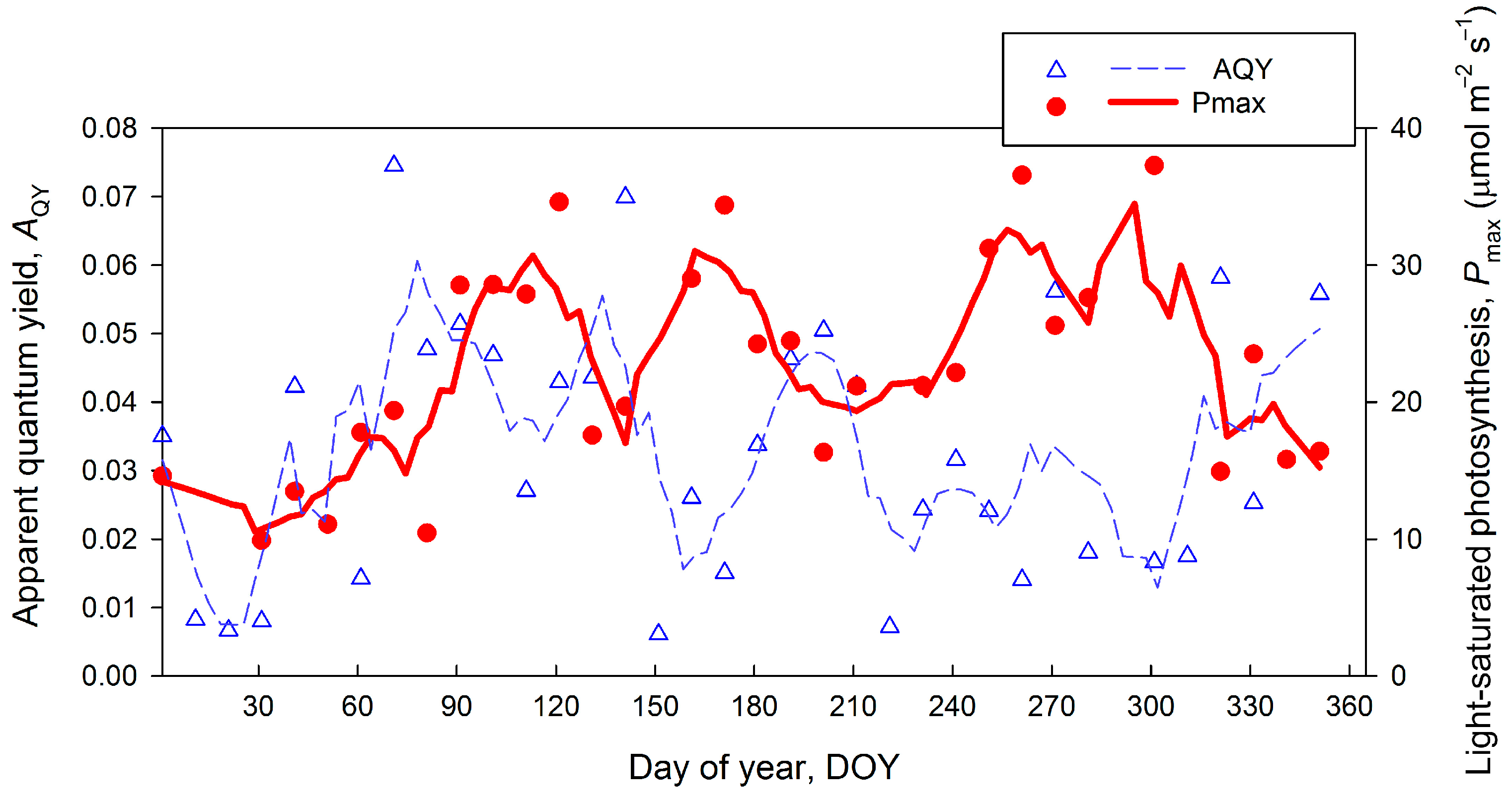
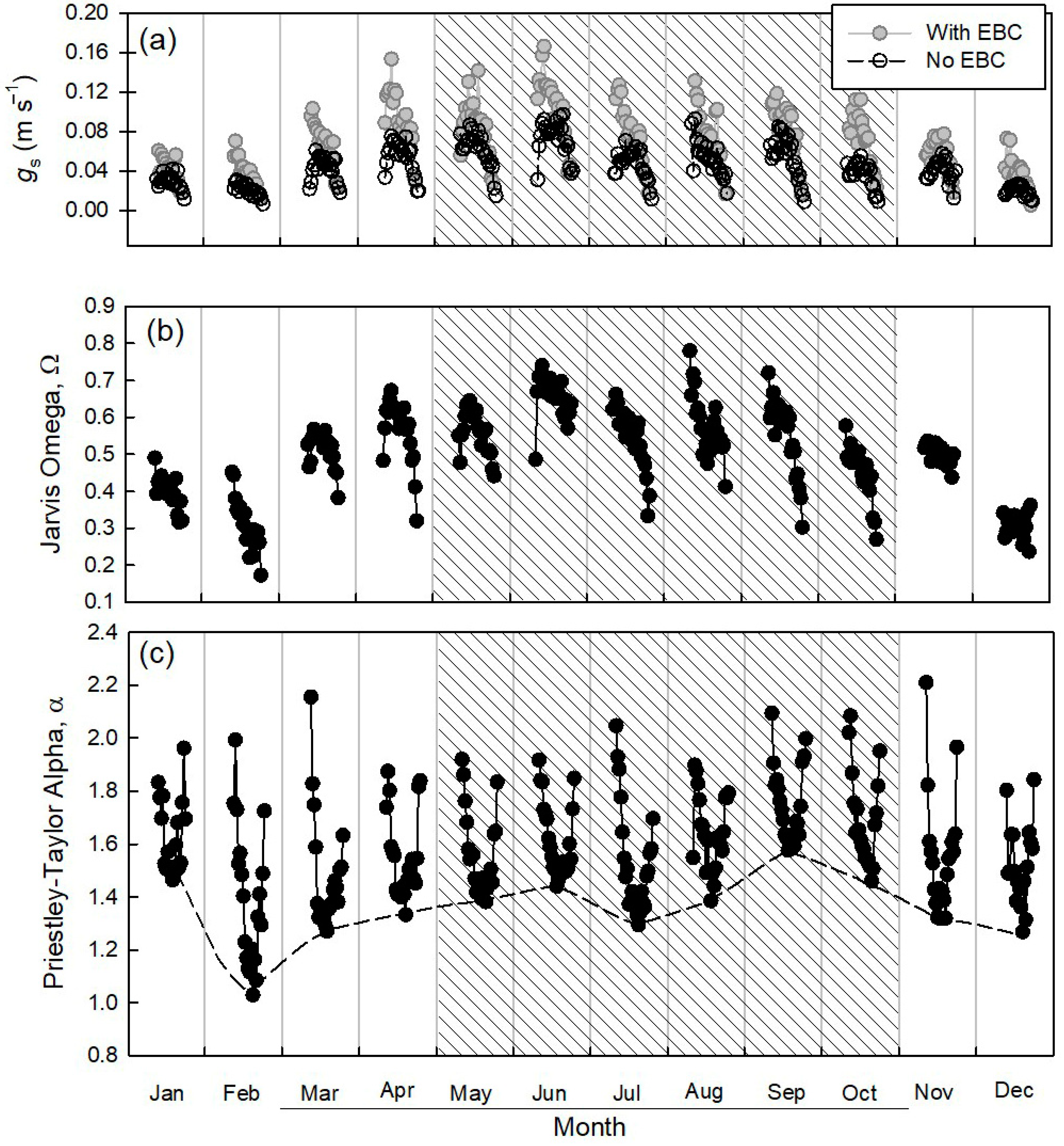
3.5. Variation of the Eddy Flux and Related Bulk Ecosystem Parameters

Figure 9a illustrates both the daytime photosynthesis carbon uptake and nighttime respiratory carbon release, and their diurnal and seasonal dynamics scale well. The carbon uptake peak occurred during April. The H dynamic differs from that of λE (Figure 9b,c). First, a higher H occurred from March through July, while a higher λE generally occurred during the wet season. The nighttime λE was close to zero. A negative H frequently occurred during nighttime.

The monthly mean diurnal variations of the eddy fluxes and surface conductance (g_s) are shown in Figure 10a. Both fluxes and g_s showed clear diurnal and seasonal variations. The energy imbalance correction increases g_s (see Figure 10a, grey and black circles). The maximum g_s was ~0.15 m s⁻¹, occurring in the mornings in June. The monthly mean diurnal variations of the Jarvis Omega (Ω) and Priestley–Taylor Alpha (α) are shown in Figure 10b,c. The Ω value showed a unimodal diurnal pattern. The highest value occurred in the morning. The daily Ω peak was generally higher than 0.5, except in the period during the middle dry season with temperatures as low as ~10 °C. On the contrary, the diurnal pattern of α exhibited a “V” style. The lowest α was generally higher than 1.0 and mostly higher than 1.2.

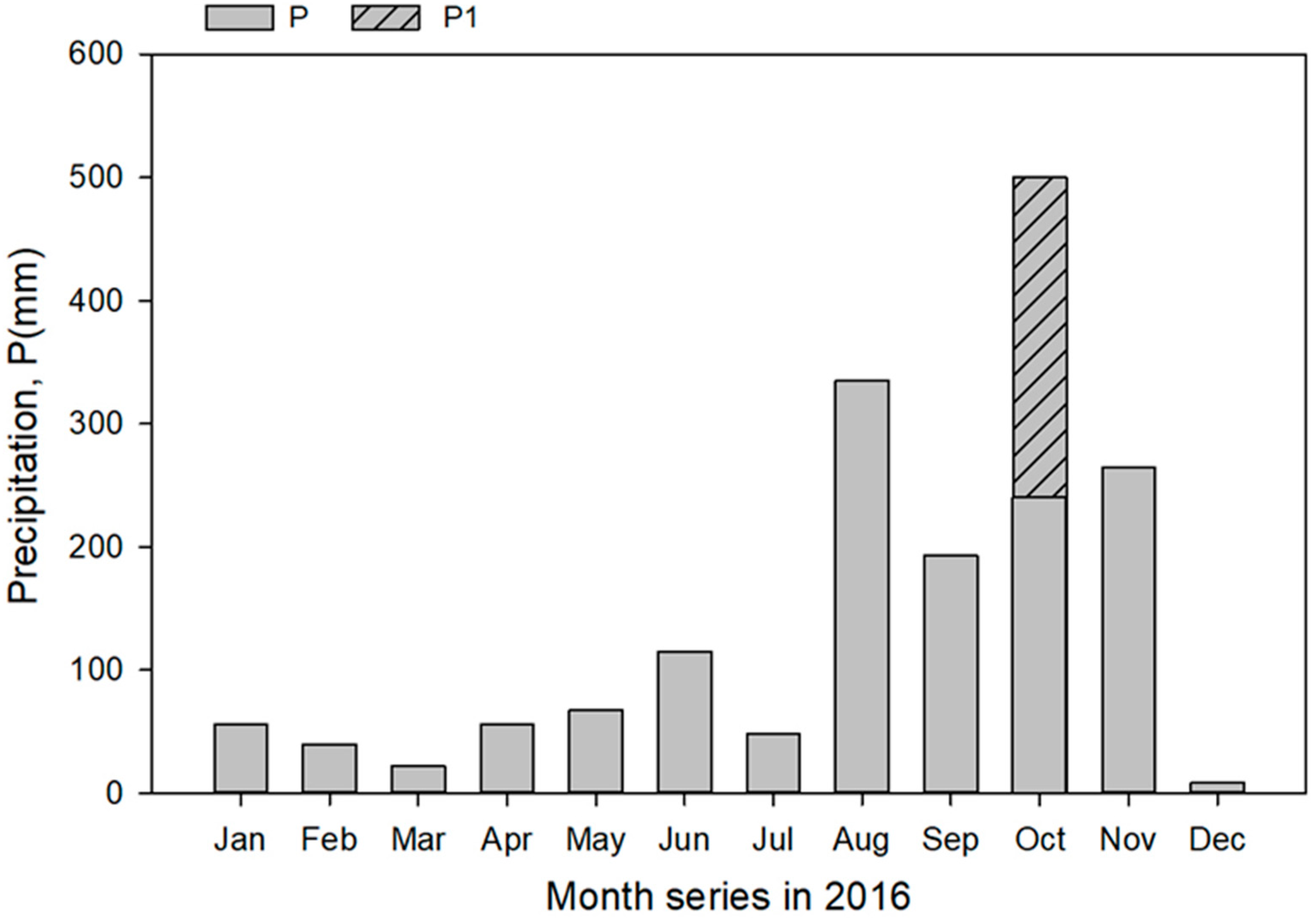
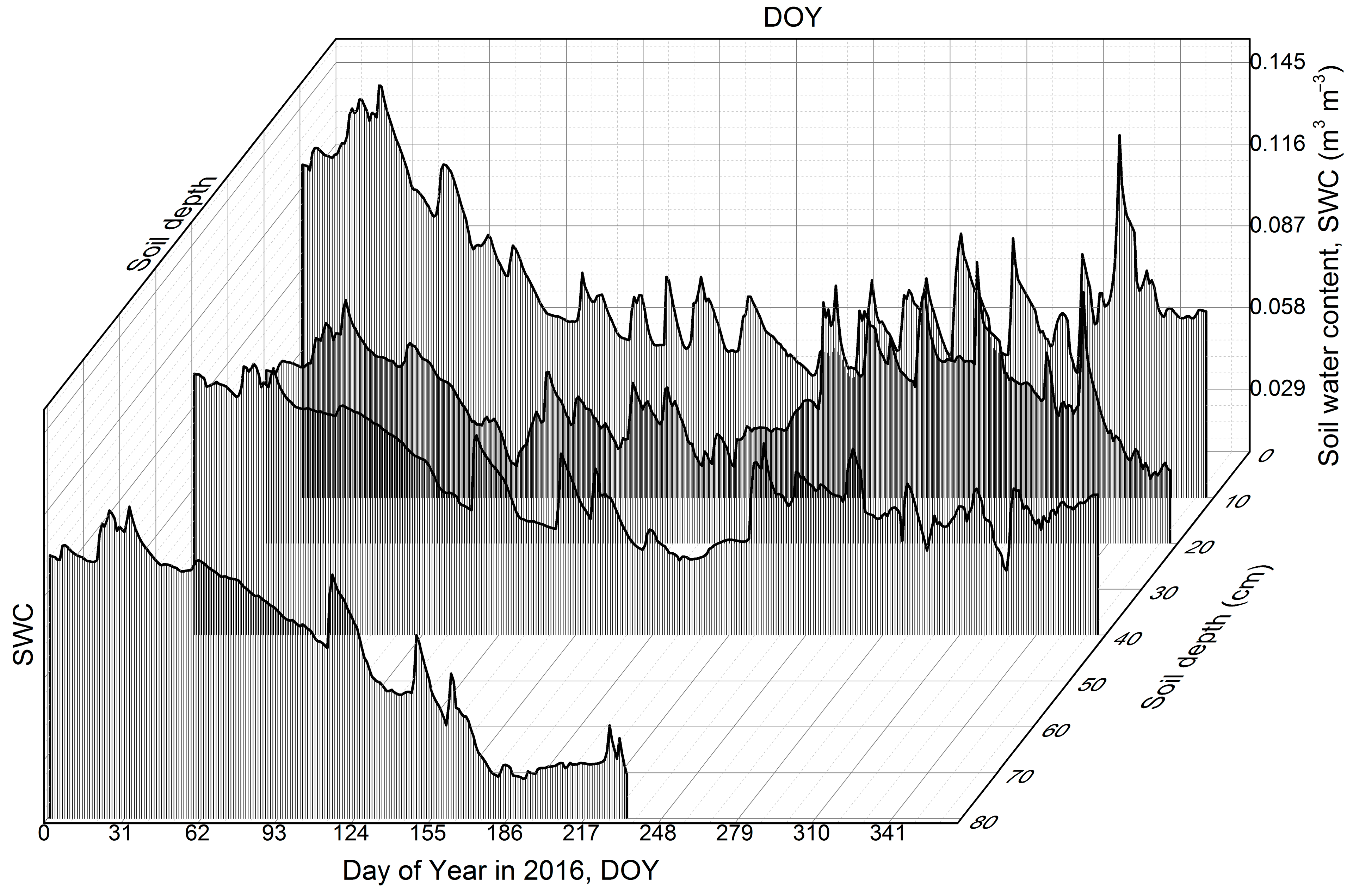
3.6. Sandy Soil Water Content Dynamics

The soil water content (SWC) had a clear seasonal pattern in all four measurement depths (Figure 11). The SWC was consistently higher in the dry season than in the wet season at all four depths. The highest SWC value (~0.13 m³ m⁻³) occurred at the shallowest depth (10 cm) at the beginning of 2016. At a depth of 80 cm, the decrease in the SWC from the dry to the wet season was most notable (from 0.11 to 0.02 m³ m⁻³).

4. Discussion

This is a pioneer study, probably the first, investigating the eddy flux over a tropical sandy coastal plain. Rather than an observational report, we present a full uncertainty analysis of the water and carbon fluxes and try to understand the gas exchange behavior in the context of the conductance-based big-leaf model. Some new findings require further discussion, which is provided below.

4.1. Uncertainties of Eddy Covariance Observations at This Study Site

We used commonly utilized commercial sensors and software to measure and process the data. We also performed a thorough uncertainty analysis. The major information of this uncertainty analysis can be summarized as follows:

The energy non-closure has an impact on both E and g_s estimations (Figure 8b and Figure 10a). Many studies have been conducted on the energy non-closure phenomenon of EC monitoring systems, and the reasons for this can be divided into two categories: overestimation of available energy and underestimation of turbulent energy [45]. Possible reasons for the overestimation of available energy include overestimation of Rn measurements and underestimation of energy storage items such as soil, air, and vegetation [46]. Possible reasons for the underestimation of turbulent energy are as follows: neglect of complex or heterogeneous surface advection [47], the loss of high- and low-frequency turbulent energy due to the instruments themselves, and sampling time [46,48]. In addition, researchers also analyzed other environmental factors or fluxes that affect energy closure. Wilson et al. [49] found that under a certain photosynthetically active radiation level, the smaller the CO₂ flux, the larger the EBC. Franssen et al. [50] found that EBC is closely related to atmospheric stability and frictional wind speed. Our knowledge about the real reason causing this energy imbalance is limited, and current explanations are incomplete. More available observation data may reduce these uncertainties to some degree.

4.2. Physiological Ecosystem Parameters

Over 90% of the signal sensed by the eddy covariance covered a distance of 500 m, as estimated by the method reported in Kljun et al. [33]. The vegetation covered within the footprint is generally similar.

The shift of the wind direction between day and night is not notable. Dominated by the monsoon climate, the predominant wind directions during the wet (southern wind) and dry seasons (northeastern wind) are contrasting. Both the southern and northern wind directions have similar vegetation covers [28].

The nighttime NEE underestimation is not large at our study site due to the strong wind and turbulence. The u_* filtering could solve this underestimation and provides a reliable NEE estimation (Figure 6a).

We performed necessary NEE and E corrections and estimated g_s.

Because there was no long data gap in our dataset, we filled the data gap of the mean diurnal variation method with a window size of 10 days. In general, both Figure 3 and a comparison of pre- and post-gap-filled data suggest that this is acceptable.

We calculated several bulk physiological ecosystem parameters, namely the apparent quantum yield (A_QY), maximum photosynthesis rate (P_max), temperature sensitivity index (Q₁₀), canopy surface conductance (g_s), Jarvis decoupling factor (Ω), and Priestley–Taylor coefficient (α). We compared our estimations with previous publications. The physiological ecosystem parameters are listed in Table 2.

Based on the plant physiology, eight photons were required to assimilate one CO₂ molecule. Thus, the theoretical maximum α is 0.125. Our estimate is 0.026, which is comparable to that of estimates for other vegetation. The Scots pine’s α is 0.027, and mixed oak’s α is 0.033 [51].

The estimated P_max of 19.87 μmol m⁻² s⁻¹ is higher than that of boreal forests (11–15 μmol m⁻² s⁻¹) but lower than that of tropical forests (20–35 μmol m⁻² s⁻¹). Boreal jack pine forests’ P_max is 13.1 μmol m⁻² s⁻¹, and tropical forests’ P_max is 29.7μmol m⁻² s⁻¹ [51].

The commonly suggested Q₁₀ value is 2.0. Bond-Lamberty et al. [52] reviewed soil respiration data and suggested a Q₁₀ value of 1.5. Mahecha et al. [53] derived an ecosystem respiration Q₁₀ of 1.4. Our estimated Q₁₀ is 2.918, which is much higher than the above-mentioned values. This indicates a strong temperature sensitivity of the ecosystem respiration of our studied vegetation.

Our estimated maximum g_s of 0.015 m s⁻¹ is close to mean global vegetation values [54] but lower than that of tropical forests [55,56]. The g_s can be viewed as the bulk stomatal conductance. Given the low leaf area index of the studied site, it is reasonable to obtain a g_s lower than that of typical tropical forests with heavy and dense canopies.

Table 2. Physiological ecosystem parameters.

Forest	AQY	Pmax	gs	α	Reference
Daodong forest farm	0.026	19.87	0.015	1.477
Scots pine	0.027	14.5			[49]
Mixed oak	0.033	24.54			[49]
Boreal forest	0.040	13.1		1.22	[49,55]
Tropical forest	0.034	29.7	0.8		[49,53,54]
Mean global vegetation values			0.018		[52]

Table 2. Physiological ecosystem parameters.

Forest	AQY	Pmax	gs	α	Reference
Daodong forest farm	0.026	19.87	0.015	1.477
Scots pine	0.027	14.5			[49]
Mixed oak	0.033	24.54			[49]
Boreal forest	0.040	13.1		1.22	[49,55]
Tropical forest	0.034	29.7	0.8		[49,53,54]
Mean global vegetation values			0.018		[52]

The Jarvis Ω describes the relative contribution of radiative (denoted as equilibrium evaporation) and advective energy (imposed evaporation) to E. When Ω approaches 0, the vegetation surface and the free air stream above are perfectly coupled [57]. The stomatal control decreases when Ω increases to 1; that is to say, stomatal control of transpiration grows progressively weaker as Ω approaches 1. The peak Ω occurs in the early morning, which suggests that the stomatal control on E is weakest in that period. In general, the stomatal control is lower in the wet season than in the dry season. This is consistent with the vegetation activities as indicated by daytime photosynthesis (Figure 9a). This pattern is very similar to that observed in boreal [58] and tropical forests [56].

We calculated the Priestley–Taylor α as $\alpha =\lambda E/[(\lambda E+H)(\Delta /(\Delta +\gamma ))]$ to avoid the impact of energy imbalance. The original expression for α is $\alpha =\lambda E/[(R_{\mathrm{n}}-G)(\Delta /(\Delta +\gamma ))]$. α increases with g_s, as described by Monteith [59]. The nonlinear fitted equation is $\alpha =1.477[1-\exp (-g_s/0.004)]$. The parameter 1.477 is higher than the previously suggested value of 1.26 obtained for boreal forests [58].

The overall energy balance closure ratio(calculated as (λE + H)/(Rn − G)) is ~75% [28], which is comparable with other studies [46].

4.3. Can the Studied Ecosystem Act as a Persistent Carbon Sink?

The study site, which is located on a sandy coastal plain, fits the requirements of eddy flux measurements well: a plain, homogenous surface, and relatively strong winds.

Our results showed the carbon sink intensity is about −560 gC m⁻² yr⁻¹. Moreover, the natural vegetation has not reached the top level of succession, and there is a certain proportion of vigorously growing artificial forests and agricultural land. Thus, it is expected that sandy coastal soil vegetation will still act as a carbon sink in the future.

We also noticed that the ecosystem respiration of the studied vegetation is small. The highest value in the wet season was only ~5 μmol m⁻² s⁻¹. At the same time, photosynthesis uptake was observed to be as high as ~20 μmol m⁻² s⁻¹. The low ecosystem respiration can be attributed to several reasons. The foremost is the low carbon density of sandy soil. The sandy coastal soil carbon density was estimated to be 7.9–14.67 t ha⁻¹ [32]. This value is much smaller than that of primary tropical mountain forests on Hainan Island [60]. Low soil respiration is expected for low-carbon-density soils. The second possible reason is the poor water storage capacity of sandy soil. As reported before, the low soil water concentration could substantially inhibit soil respiration in tropical regions [61]. This might be the second reason leading to low ecosystem respiration. The third reason is related to the predominant species Casuarina equisetifolia. Casuarina equisetifolia (also called Australian pine tree) is naturally distributed in Australia and was introduced and widely planted in Hainan in the past years as a tree species for constructing windbreaks in sandy coastal regions [62]. Casuarina equisetifolia leaves are similar to needles and difficult to decompose compared with other broadleaved species. Additionally, EC instrumentation error could also be one possible reason as only one-year data were available in the studied site.

The inhibited respiration in sandy soil and the secondary growth, both of planted trees and natural succession after disturbance, will sustain this carbon sink for years, i.e., one or two decades. Given that the sequestrated carbon is mainly stored in vegetation biomass, the biomass will increase by ~100 t C ha⁻¹ after 20 years. It is reasonable for tropical vegetation to store 200–300 t C ha⁻¹ of carbon in their biomass [63]. However, low soil water density and soil carbon stock were observed in the study site, which might interrupt the continuous growth of tall trees. In this case, the forest may stop its growth at a relatively low height in the future.

4.4. Unexpected Seasonal Soil Water Content Pattern and Its Possible Explanation

As over 80% of the precipitation occurs during the wet season, it is more likely that higher soil water contents in the wet season are observed than in the dry season, which is also common in tropical areas [64]. Conversely, the soil water content observed at our site was higher in the dry season than in the rainy season (Figure 11). After confirming that this pattern was not caused by measurement errors, we tried to understand it in the context of soil water balance. Compared with other soil types, the water storage capacity of sandy soil is very poor. In addition, plant roots might access deep soil water to maintain continuously high transpiration during the wet season. The above factors lead to a soil water deficit in the wet season. This explanation can be partially supported with Figure 8b. The annual precipitation during the study year was lower than the multi-year mean value recorded at the Wenchang weather station (1721 mm). In the wet season before September, the evapotranspiration (E) value was higher than the precipitation, illustrating a soil water deficit. Another possible explanation was related to human activities. The study site was adjacent to several ponds and paddy fields, and human activities such as irrigation or drainage or groundwater inflow from surrounding land surfaces could induce disturbances to SWC; however, we believed that the extent of disturbances from human activities was relatively small compared with other environmental factors such as soil type and root water absorption as the area of the forest was much larger than that of the nearby ponds and paddy fields. Certainly, a well-designed study on the soil water balance will provide a more solid explanation of this unexpected pattern.

4.5. Possible Explanation of the Strongest Carbon Assimilation in the Late Dry Season Shortly before Rainfall Starts and Its Implications

The photosynthesis carbon assimilation was highest in April, shortly before the rainy season (Figure 6 and Figure 9a). The E value of the corresponding time did not reach its peak value (Figure 9c). In this period, the soil water content is at its median level compared with other months over the year (Figure 11). Why did the photosynthesis peak in April? Is it caused by endogenous or exogenous factors? We suspect that endogenous factors play a leading role in this case. Plants seemingly adjust themselves to an optimum stage when waiting for rainfall and reach a greater photosynthesis gain during the wet season [65]. Additionally, water-use strategies may vary by species and their location on the landscape [66]. Although located in the south of the Tropic of Cancer, the latitude of the study site is 19°43′ N. Combined with the monsoon climate, plants of the studied vegetation grow under a climate with clear seasonality both with respect to water and temperature. Approaching April, the temperature rose to near peak levels and some rainfall had already occurred (Figure 8b). The soil water content still retained median levels. This certainly is an optimal climate for photosynthesis. Plants growing under such an environment evolve a special adjustment ability to better utilize these climatic conditions. A further control experiment might provide more solid support for this hypothesis.

5. Conclusions

We report one-year eddy flux observations over a tropical sandy coastal plain. After detailed analysis, we draw the following conclusions: Both the daily peak Rn and the λE showed similar seasonal variations, with a higher value in the wet season than in the dry season. The soil heat flux (G) was comparable to the values of H and λE, implying the open canopy of the study site may strongly affect the energy allocation. The PAR explained approximately 45% of the daytime NEE variance. In general, the studied ecosystem was a carbon sink (approximately −560 gC m⁻² yr⁻¹). The carbon sink nature was mainly due to the plain’s rapid secondary growth after several typhoons and the low soil respiration of sandy soil. The annual evapotranspiration estimate varied from 940 to 1020 mm based on different calculations, which was around 70% of the precipitation for this region. Both fluxes and gs showed clear diurnal and seasonal variations. The maximum gs was ~0.15 m s⁻¹, occurring in the mornings in June. The Ω value showed a unimodal diurnal pattern with the highest value occurring in the morning, while the diurnal pattern of α exhibited an opposite pattern. Peak photosynthesis occurred in the period shortly before the start of the wet season. This can be explained as an endogenous self-adjustment to improve the water- and carbon-use efficiency during the wet season.

References

1. Kondo, M.; Saitoh, T.M.; Sato, H.; Ichii, K. Comprehensive synthesis of spatial variability in carbon flux across monsoon Asian for-ests. Agric. For. Meteorol. 2017, 232, 623–634. [Google Scholar] [CrossRef] [Green Version]
2. Hirata, R.; Saigusa, N.; Yamamoto, S.; Ohtani, Y.; Ide, R.; Asanuma, J.; Gamo, M.; Hirano, T.; Kondo, H.; Kosugi, Y.; et al. Spatial distribution of carbon balance in forest ecosystems across East Asia. Agri-Cult. For. Meteorol. 2008, 148, 761–775. [Google Scholar] [CrossRef]
3. Jin, Y.; Liu, Y.; Liu, J.; Zhang, X. Energy Balance Closure Problem over a Tropical Seasonal Rainforest in Xishuangbanna, Southwest China: Role of Latent Heat Flux. Water 2022, 14, 395. [Google Scholar] [CrossRef]
4. Dennis, B. Measuring fluxes of trace gases and energy between ecosystems and the atmosphere—The state and future of the eddy covariance method. Glob. Chang. Biol. 2015, 20, 3600–3609. [Google Scholar]
5. Zeri, M.; Sá, L.; Manzi, A.; Araújo, A.; Aguiar, R.; von Randow, C.; Sampaio, G.; Cardoso, F.; Nobre, C. Variability of carbon and water fluxes following climate extremes over a tropical forest insouthwestern Amazonia. PLoS ONE 2014, 9, e88130. [Google Scholar] [CrossRef] [Green Version]
6. Yamanoi, K.; Mizoguchi, Y.; Utsugi, H. Effects of a windthrow disturbance on the carbon balance of a broadleaf deciduous forest in Hokkaido, Japan. Biogeosci. Discuss. 2015, 12, 10425–10468. [Google Scholar] [CrossRef] [Green Version]
7. Baldocchi, D.; Chu, H.; Reichstein, M. Inter-annual variability of net and gross ecosystem carbon fluxes: A review. Agricul-Tural For. Meteorol. 2017, 249, 520–538. [Google Scholar] [CrossRef] [Green Version]
8. Dunn, A.L.; Barford, C.C.; Wofsy, S.C.; Goulden, M.L.; Daube, B.C. A long-term record of carbon exchange in a boreal black spruce forest: Means, responses to in terannual variability, and decadal trends. Glob. Chang. Biol. 2007, 13, 577–590. [Google Scholar] [CrossRef] [Green Version]
9. Ilvesniemi, H.; Levula, J.; Ojansuu, R.; Kolari, P.; Kulmala, L.; Pumpanen, J.; Launiainen, S.; Vesala, T.; Nikinmaa, E. Long-term measurements of the carbon balance of a boreal Scots pine dominated forest ecosystem. Boreal Environ. Res. 2009, 14, 731–753. [Google Scholar]
10. Richardson, A.D.; Hollinger, D.Y.; Aber, J.D.; Ollinger, S.V.; Braswell, B.H. Environmental variation is directly responsible for short- but not long-term variation in forest-atmosphere carbon exchange. Glob. Chang. Biol. 2007, 13, 788–803. [Google Scholar] [CrossRef]
11. Soloway, A.D.; Amiro, B.D.; Dunn, A.L.; Wofsy, S.C. Carbon neutral or a sink? Uncertainty caused by gap-filling long-term flux measurements for an old-growth boreal black spruce forest. Agric. For. Meteorol. 2017, 233, 110–121. [Google Scholar] [CrossRef]
12. Ueyama, M.; Iwata, H.; Harazono, Y. Autumn warming reduces the CO2 sink of a black spruce forest in interior Alaska based on a nine-year eddy covariance mea surement. Glob. Chang. Biol. 2014, 20, 1161–1173. [Google Scholar] [CrossRef] [PubMed]
13. Amiro, B.D.; Barr, A.G.; Barr, J.G.; Black, T.A.; Bracho, R.; Brown, M.; Chen, J.; Clark, K.L.; Davis, K.J.; Desai, A.R.; et al. Ecosystem carbon dioxide fluxes after disturbance in forests of North America. J. Geophys. Res. 2010, 115. [Google Scholar] [CrossRef] [Green Version]
14. Goulden, M.L.; Mcmillan, A.M.S.; Winston, G.C.; Rocha, A.V.; Manies, K.L.; Harden, J.W.; Bond-Lamberty, B.P. Patterns of NPP, GPP, respiration, and NEP during boreal forest succession. Glob. Chang. Biol. 2011, 17, 855–871. [Google Scholar] [CrossRef] [Green Version]
15. Jarvis, P.G.; Leverenz, J. Productivity of temperate, deciduous and evergreen forests. In Encyclopedia of Plant Physiology; Eal, O.L., Ed.; Springer: Berlin/Heidelberg, Germany, 1983. [Google Scholar]
16. Bracho, R.; Starr, G.; Gholz, H.L.; Martin, T.A.; Cropper, W.P.; Loescher, H.W. Controls on carbon dynamics by ecosystem structure and climate for southeastern U. S:slash pine plantations. Ecol. Monogr. 2012, 82, 101–128. [Google Scholar] [CrossRef]
17. Dore, S.; Montes-Helu, M.; Hart, S.C.; Hungate, B.A.; Koch, G.W.; Moon, J.B.; Finkral, A.J.; Kolb, T.E. Recovery of ponderosa pine ecosystem carbon and water fluxes from thinning and stand-replacing fire. Glob. Chang. Biol. 2012, 18, 3171–3185. [Google Scholar] [CrossRef]
18. Froelich, N.; Croft, H.; Chen, J.M.; Gonsamo, A.; Staebler, R.M. Trends of carbon fluxes and climate over a mixed temperate-boreal transition forest in southern Ontario, Canada. Agric. For. Meteorol. 2015, 211, 72–84. [Google Scholar] [CrossRef]
19. Granier, A.; Bréda, N.; Longdoz, B.; Gross, P.; Ngao, J. Ten years of fluxes and stand growth in a young beech forest at Hesse, North-eastern France. Ann. For. Sci. 2008, 65, 704. [Google Scholar] [CrossRef] [Green Version]
20. Herbst, M.; Mund, M.; Tamrakar, R.; Knohl, A. Differences in carbon uptake and water use between a managed and an unmanaged beech forest in central Germany. For. Ecol. Manag. 2015, 355, 101–108. [Google Scholar] [CrossRef]
21. Novick, K.; Oishi, C.; Ward, E.; Siqueira, M.; Juang, J.-Y.; Stoy, P. On the difference in the net ecosystem exchange of CO2 between deciduous and evergreen forests in the southeastern United States. Glob. Chang. Biol. 2015, 21, 827–842. [Google Scholar] [CrossRef] [Green Version]
22. Pilegaard, K.; Ibrom, A.; Courtney, M.S.; Hummelshøj, P.; Jensen, N.O. Increasing net CO2 uptake by a Danish beech forest during the period from 1996 to 2009. Agric. For. Meteorol. 2011, 151, 934–946. [Google Scholar] [CrossRef]
23. Baumgartner, A. Meteorological approach to the exchange of CO2 between the atmosphere and vegetation, particularly foreststands. Photosynthetica 1969, 3, 127–149. [Google Scholar]
24. Denmead, O.T. Comparative micrometeorology of a wheat field and a forest of Pinus radiata. Agric. Meteorol. 1969, 6, 357–371. [Google Scholar] [CrossRef]
25. Speckman, H.; Frank, J.; Bradford, J.; Miles, B.; Massman, W.; Parton, W.; Ryan, M. Forest ecosystem respiration estimated from eddy covariance and chambermeasurements under high turbulence and substantial tree mortality from bark beetles. Glob. Chang. Biol. 2015, 21, 708–721. [Google Scholar] [CrossRef]
26. Shan, J. Study on the spermatophyte flora of the coastal sandy region of hainan island. Guangdong For. Ence Technol. 2008, 24, 37–40. [Google Scholar]
27. Herrmann, M.; Najjar, R.G.; Kemp, W.M.; Alexander, R.B.; Boyer, E.W.; Cai, W.-J.; Griffith, P.C.; Kroeger, K.D.; McCallister, S.L.; Smith, R.A. Net ecosystem production and organic carbon balance of US East Coast estu-aries: A synthesis approach. Glob. Biogeochem. Cycles 2015, 29, 96–111. [Google Scholar] [CrossRef]
28. Xue, Y.; Yang, Z.Y.; Su, S.F.; Wang, X.Y.; Lin, Z.P.; Zhao, J.F.; Tan, Z.H. A preliminary report on mass and energy flux over a coastal vegetation in Hainan Island. Trop. For. 2016, 44, 48–52, (In Chinese with English abstract). [Google Scholar]
29. Xue, Y.; Yang, Z.Y.; Chen, Y.Q.; Wang, X.Y.; Su, S.F.; Lin, Z.P.; Lin, R.W.; Xue, Y.W. Characteristics of soil organic carbon and litter of typical forest types in tropical coastal zone. Chin. J. Trop. Crops 2016, 37, 2083–2088, (In Chinese with English abstract). [Google Scholar]
30. Verma, S.B. Micrometeorological methods for measuring surface fluxes of mass and energy. Remote Sens. Rev. 1990, 5, 99–115. [Google Scholar] [CrossRef]
31. Wilczak, J.M.; Oncley, S.P.; Stage, S.A. Sonic anemometer tilt correction algorithms. Bound. Layer Meteorol. 2001, 99, 127–150. [Google Scholar] [CrossRef]
32. Webb, E.K.; Pearman, G.I.; Leuning, R. Correction of flux measurements for density effect due to heat and water vapor transfer. Q. J. R. Meteorol. Soc. 1980, 106, 85–100. [Google Scholar] [CrossRef]
33. Kljun, N.; Calanca, P.; Rotach, M.W.; Schmid, H.P. A simple parameterization for flux footprint predictions. Bound. Layer Meteorol. 2004, 112, 503–523. [Google Scholar] [CrossRef]
34. Moncrieff, J.B.; Massheder, J.M.; de Bruin, H.; Ebers, J.; Friborg, T.; Heusinkveld, B.; Kabat, P.; Scott, S.; Soegaard, H.; Verhoef, A. A system to measure surface fluxes of momentum, sensible heat, water vapor and carbon dioxide. J. Hydrol. 1997, 188–189, 589–611. [Google Scholar] [CrossRef]
35. Vickers, D.; Mahrt, L. Quality control and flux sampling problems for tower and aircraft data. J. Atmos. Ocean. Technol. 1997, 14, 512–526. [Google Scholar] [CrossRef]
36. Saleska, S.R.; Miller, S.D.; Matross, D.M.; Goulden, M.L.; Wofsy, S.C.; da Rocha, H.; de Camargo, P.B.; Crill, P.M.; Daube, B.C.; Freitas, C.L.; et al. Carbon in Amazon forests: Unexpected seasonal fluxes and disturbance-induced losses. Science 2003, 302, 1554–1557. [Google Scholar] [CrossRef] [Green Version]
37. Falge, E.; Baldocchi, D.; Olson, R.; Anthoni, P.; Aubinet, M.; Bernhofer, C.; Burba, G.; Ceulemans, R.; Clement, R.; Dolman, H.; et al. Gap filling strategies for long term energy flux data sets. Agric. For. Meteorol. 2001, 107, 71–77. [Google Scholar] [CrossRef] [Green Version]
38. Penman, H.L. Natural evaporation from open water, bare soil and grass. Proc. R. Soc. A Math. Phys. Eng. Sci. 1948, 193, 120–145. [Google Scholar]
39. Verma, S.B. Aerodynamic resistances to transfers of heat, mass and momentum. In Estimation of Areal Evapotranspiration; Black, T.A., Spittlehouse, D.L., Novak, M.D., Price, D.T., Eds.; IAHS Publication: Vancouver, BC, Canada, 1989; pp. 13–20. [Google Scholar]
40. Paulson, C.A. The mathematical representation of wind speed and temperature profiles in the unstable atmospheric surface layer. J. Appl. Meteorol. 1970, 9, 857–861. [Google Scholar] [CrossRef]
41. Falge, E.; Baldocchi, D.; Olson, R.; Anthoni, P.; Tu, K. Gap filling strategies for defensible annual sums of net ecosystem exchange. Agric. For. Meteorol. 2001, 107, 43–69. [Google Scholar] [CrossRef] [Green Version]
42. Hoff, J.H.; Lehfeldt, R.A. Lectures on Theoretical and Physical Chemistry. Nature 1900, 62, 245. [Google Scholar]
43. Jarvis, P.G.; McNaughton, K.G. Stomatal control of transpiration: Scaling up from leaf to region. Adv. Ecol. Res. 1986, 15, 1–49. [Google Scholar]
44. Priestley, C.B.H.; Taylor, R.J. On the assessment of surface heat flux and evaporation using large scale parameters. Mon. Weather. Rev. 1972, 100, 81–92. [Google Scholar] [CrossRef]
45. McGloin, R.; Šigut, L.; Havránková, K.; Dušek, J.; Pavelka, M.; Sedlák, P. Energy balance closure at a variety of ecosystems in Central Europe with contrasting topographies. Agric. For. Meteorol. 2018, 248, 418–431. [Google Scholar] [CrossRef]
46. Foken, T. The energy balance closure problem: An overview. Ecol. Appl. 2008, 18, 1351–1367. [Google Scholar] [CrossRef]
47. Oncley, S.P.; Foken, T.; Vogt, R.; Kohsiek, W.; Debruin, H.A.R.; Bernhofer, C.; Christen, A.; van Gorsel, E.; Grantz, D.; Feigenwinter, C.; et al. The Energy Balance Experiment EBEX-2000. Part I: Overview and energy balance. Bound. Layer Meteorol. 2007, 123, 1–28. [Google Scholar] [CrossRef]
48. Leuning, R.; van Gorsel, E.; Massman, W.J.; Isaac, P.R. Reflections on the surface energy imbalance problem. Agric. For. Meteorol. 2012, 156, 65–74. [Google Scholar] [CrossRef]
49. Wilson, K.; Goldstein, A.; Falge, E.; Aubinet, M.; Baldocchi, D.; Berbigier, P.; Bernhofer, C.; Ceulemans, R.; Dolman, H.; Field, C.; et al. Energy balance closure at FLUXNET sites. Agric. For. Meteorol. 2002, 113, 223–243. [Google Scholar] [CrossRef] [Green Version]
50. Franssen, H.J.H.; Stockli, R.; Lehner, I.; Rotenberg, E.; Seneviratne, S.I. Energy balance closure of eddy-covariance data: A multisite analysis for European FLUXNET stations. Agric. For. Meteorol. 2010, 150, 1553–1567. [Google Scholar] [CrossRef]
51. Zhang, L.-M.; Yu, G.-R.; Sun, X.-M.; Wen, X.-F.; Ren, C.-Y.; Fu, Y.-L.; Li, Q.-K.; Li, Z.-Q.; Liu, Y.-F.; Guan, D.-X.; et al. Seasonal variations of ecosystem apparent quantum yield (α) and maximum photosynthesis rate (Pmax) of different forest ecosystems in China. Agric. For. Meteorol. 2006, 137, 176–187. [Google Scholar] [CrossRef]
52. Bond-Lamberty, B.; Thomson, A. Temperature-associated increases in the global soil respiration record. Nature 2010, 464, 579–582. [Google Scholar] [CrossRef]
53. Mahecha, M.; Reichstein, M.; Carvalhais, N.; Lasslop, G.; Lange, H.; Seneviratne, S.; Vargas, R.; Ammann, C.; Arain, A.; Cescatti, A.; et al. Global convergence in the temperature sensitivity of respiration at ecosystem level. Science 2010, 329, 838–840. [Google Scholar] [CrossRef] [Green Version]
54. Kelliher, F.M.; Leuning, R.; Raupach, M.R.; Schulze, E.D. Maximum conductances for evaporation from global vegetation types. Agric. For. Meteorol. 1995, 73, 1–16. [Google Scholar] [CrossRef]
55. Grace, J.; Lloyd, J.; McIntyre, J.; Miranda, A.; Meir, P.; Miranda, H.; Moncrieff, J.; Massheder, J.; Wright, I.; Gash, J. Fluxes of carbon dioxide and water over an undisturbed tropical forest in south-west Amazonia. Glob. Chang. Biol. 1995, 1, 1–12. [Google Scholar] [CrossRef]
56. Kumagai, T.; Saitoh, T.M.; Sato, Y.; Morooka, T.; Manfroi, O.J.; Kuraji, K.; Suzuki, M. Transpiration, canopy conductance and the decoupling coefficient of a lowland mixed dipterocarp forest in Sarawak, Borneo: Dry spell effect. J. Hydrol. 2004, 287, 237–251. [Google Scholar] [CrossRef]
57. Pereira, A.R. The priestley–taylor parameter and the decoupling factor for estimating reference evapotranspiration. Agric. For. Meteorol. 2004, 125, 305–313. [Google Scholar] [CrossRef]
58. Blanken, P.D.; Black, T.A.; Yang, P.C.; Neumann, H.H.; Nesic, Z.; Staebler, R.; den Hartog, G.; Novak, M.D.; Lee, X. Energy balance and canopy conductance of a boreal aspen forest: Partitioning overstory and understory components. J. Geophys. Res. Atmos. 1997, 102, 28915–28927. [Google Scholar] [CrossRef] [Green Version]
59. Monteith, J.L. Accommodation between transpiring vegetation and the convective boundary layer. J. Hydrol. 1995, 116, 251–263. [Google Scholar] [CrossRef]
60. Yang, H.; Li, Y.-D.; Ren, H.; Luo, T.-S.; Chen, R.-L.; Liu, W.-J.; Chen, D.-X.; Xu, H.; Zhou, Z.; Lin, M.-X.; et al. Soil organic carbon density and influencing factors in tropical virgin forests of Hainan Island, China. Chin. J. Plant Ecol. 2016, 40, 292–303. [Google Scholar]
61. Takada, M.; Yamada, T.; Kadir, W.R.; Okuda, T. Spatial and temporal variation in soil respiration in a Southeast Asian tropical rainforest. Agric. For. Meteorol. 2007, 147, 35–47. [Google Scholar]
62. Xue, Y.; Yang, Z.; Wang, X.; Lin, Z.; Li, D.; Su, S. Tree biomass allocation and its model Additivity for Casuarina equisetifolia in a tropical forest of Hainan Island, China. PLoS ONE 2016, 11, e0151858. [Google Scholar] [CrossRef] [Green Version]
63. Malhi, Y.; Aragao, L.E.O.C.; Metcalfe, D.B.; Paiva, R.; Quesada, C.A.; Almeida, S.; Anderson, L.; Brando, P.; Chambers, J.Q.; da Costa, A.C.L.; et al. Comprehensive assessment of carbon productivity, allocation and storage in three Amazonian forests. Glob. Chang. Biol. 2009, 15, 1255–1274. [Google Scholar] [CrossRef]
64. da Rocha, H.R.; Manzi, A.O.; Cabral, O.M.; Miller, S.D.; Goulden, M.L.; Saleska, S.R.; Coupe, N.R.; Wofsy, S.C.; Borma, L.S.; Artaxo, P.; et al. Patterns of water and heat flux across a biome gradient from tropical forest to savanna in Brazil. J. Geophys. Res. Biogeosci. 2009, 114. [Google Scholar] [CrossRef]
65. Wu, J.; Albert, L.P.; Lopes, A.P.; Restrepo-Coupe, N.; Hayek, M.; Wiedemann, K.T.; Guan, K.; Stark, S.C.; Christoffersen, B.; Prohaska, N.; et al. Leaf development and demography explain photosynthesis seasonality in Amazon evergreen forests. Science 2016, 351, 972–976. [Google Scholar] [CrossRef] [PubMed] [Green Version]
66. Boggs, J.L.; Sun, G.; Domec, J.-C.; McNulty, S.G. Variability of tree transpiration across three zones in a southeastern US Piedmont watershed. Hydrol. Process. 2021, 35, e14389. [Google Scholar] [CrossRef]
Figure 1. Geographic Location of Study Site (left); images in study region (right).
Water 15 00877 g001
Figure 2. Illustration of nighttime carbon flux (eddy carbon flux (Fc), storage flux (Fs) and net ecosystem exchange (NEE)) underestimation due to stable weather and the determination of the threshold friction velocity (u*) for filtering. The error bars indicate standard errors.
Water 15 00877 g002
Figure 3. Net radiation (a, Rn), Sensible heat (b, H), Latent heat (c, λE), Soil heat flux (d, G). Time series of energy fluxes as observed by the eddy flux tower. The figure shows 30 min intervals for one-year data collected in 2016. No gap filling was performed.
Water 15 00877 g003
Figure 4. Monthly Dynamic Variation of Precipitation. The actual rainfall in October is P + P1, where P is the measurement data of the study area, and P1 is the data missing due to instrument failure during typhoon “Sarija”.
Water 15 00877 g004
Figure 5. Environmental response of the net ecosystem exchange (NEE). (a) Light response of the daytime NEE. A nonrectangular hyperbola equation was fitted to the data. (b) Temperature response of the nighttime NEE. The Q10 function was fitted to the data. The lines indicate the linear regression.
Water 15 00877 g005
Figure 6. Time series of the net ecosystem exchange before (a) and after gap filling (b). The figure shows 30 min intervals for one-year data collected in 2016.
Water 15 00877 g006
Figure 7. The annual variation of light response parameters with a regression window size of 10 days. AQY and Pmax represent the apparent quantum yield and light-saturated photosynthesis. The red line and blue dashed line represent the fitting curves of AQY and Pmax.
Water 15 00877 g007
Figure 8. The accumulated carbon and water fluxes. (a) accumulated carbon sequestration. The red, green, and blue lines indicate no u* filtering (u* is the friction velocity, annual sum of −649 gC m−2 s−1), a threshold u* of 0.17 m s−1 (annual sum of −559 gC m−2 s−1), and a threshold u* of 0.25 m s−1 (annual sum of −563 gC m−2 s−1), respectively. (b) accumulated water fluxes. The red, blue, pink, green, and black lines represent the accumulated water flux obtained from the Bowen ratio energy balance correction (1060 mm), gap filling the observation data (940 mm), treating all negative fluxes as zero (973 mm), treating all negative fluxes as gaps and filling the gaps (1020 mm), and the precipitation (1482 mm), respectively.
Water 15 00877 g008
Figure 9. Net ecosystem exchange (a, NEE), sensible heat flux (b, H), and latent heat flux (c, λE). The shaded area indicates the wet season (May through October).
Water 15 00877 g009
Figure 10. The monthly mean diurnal variation of the surface conductance (a, gs), Jarvis Omega (b, Ω) and Priestley–Taylor Alpha (c, α). The gs value was also calculated after energy imbalance correction, which is shown as EBC. The shaded area indicates the wet season (May through October).
Water 15 00877 g010
Figure 11. The seasonal variation of the soil water content (SWC) at different depths, shown as a waterfall figure. The SWC at an 80 cm depth had no data after the middle of the wet season due to sensor failure.
Water 15 00877 g011