
Comprehensive Methodology and Analysis to Determine the Environmental Flow Regime in the Temporary Stream “La Yerbabuena” in Aguascalientes, Mexico

 , , and
Abstract
:1. Introduction
- Define the regime of environmental flow for La Yerbabuena stream, adapting the existent methodologies for temporary streams.
- Compare the results of environmental flow obtained with the proposed methodology for temporary streams against the methodologies of existing standards.
- Apply hydraulic modeling to understand the behavior of La Yerbabuena as a temporary stream under scenarios of dry and rainy seasons.
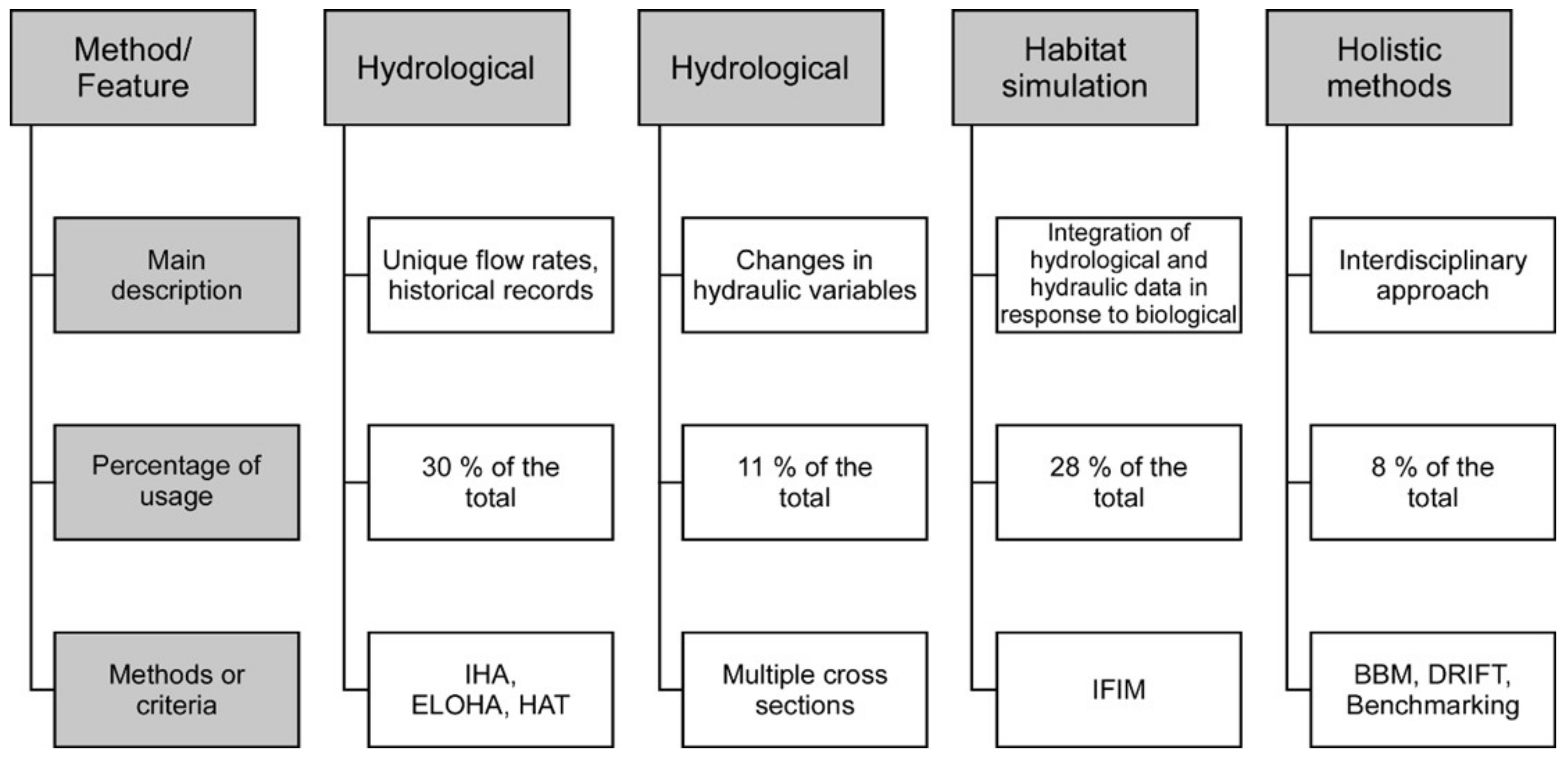
Application of the IHA Methodology for the Determination of Environmental Flows in Temporary Rivers
2. Materials and Methods
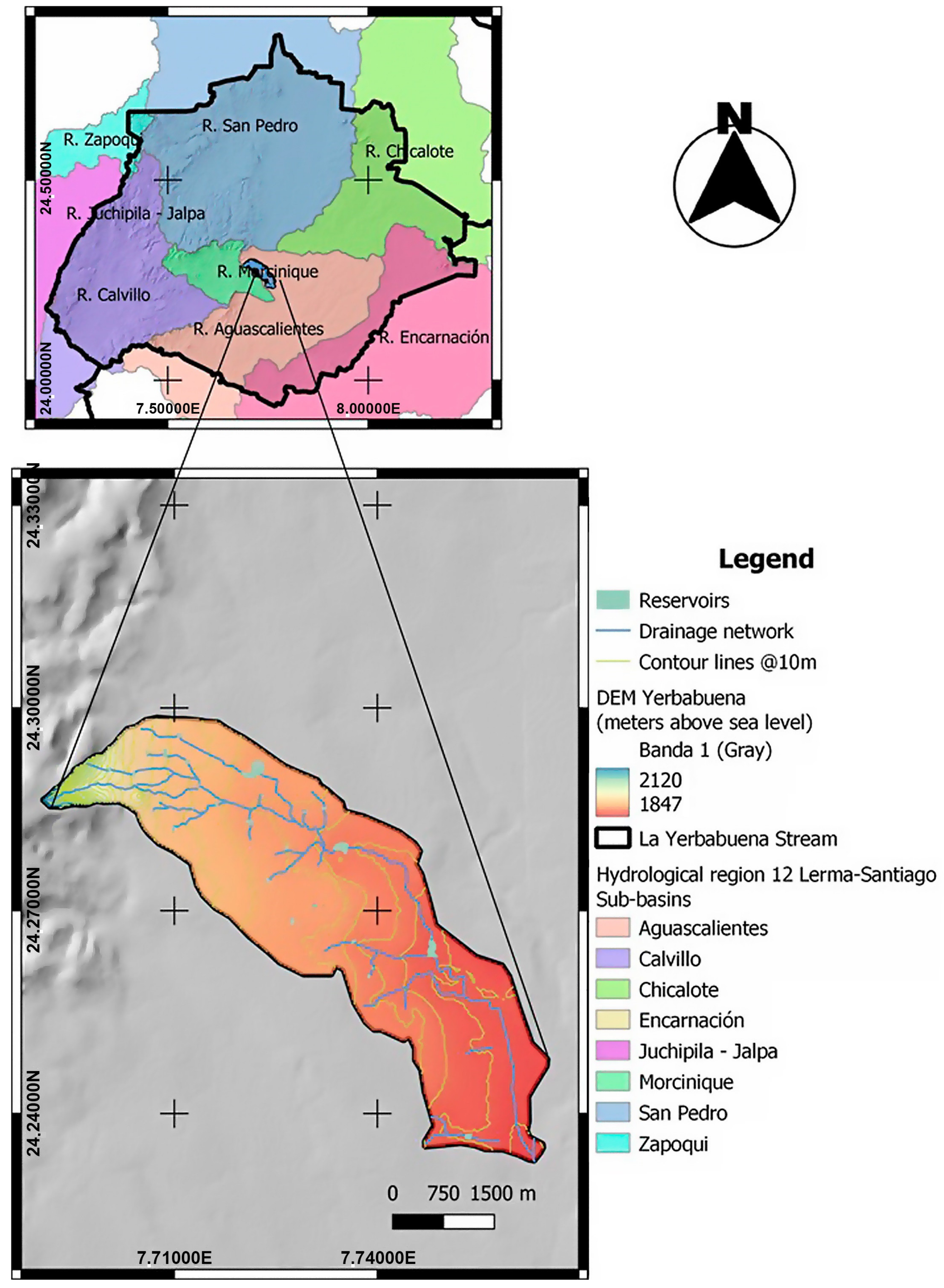
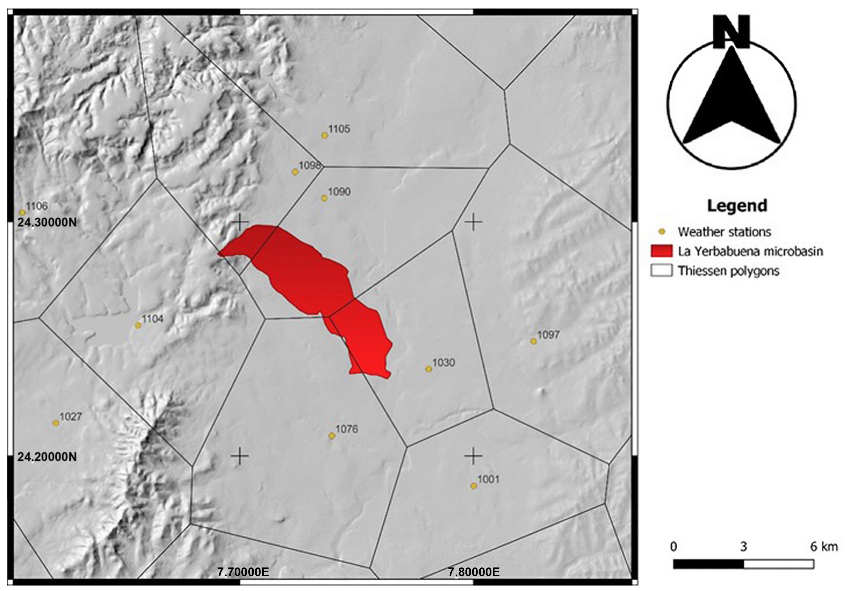
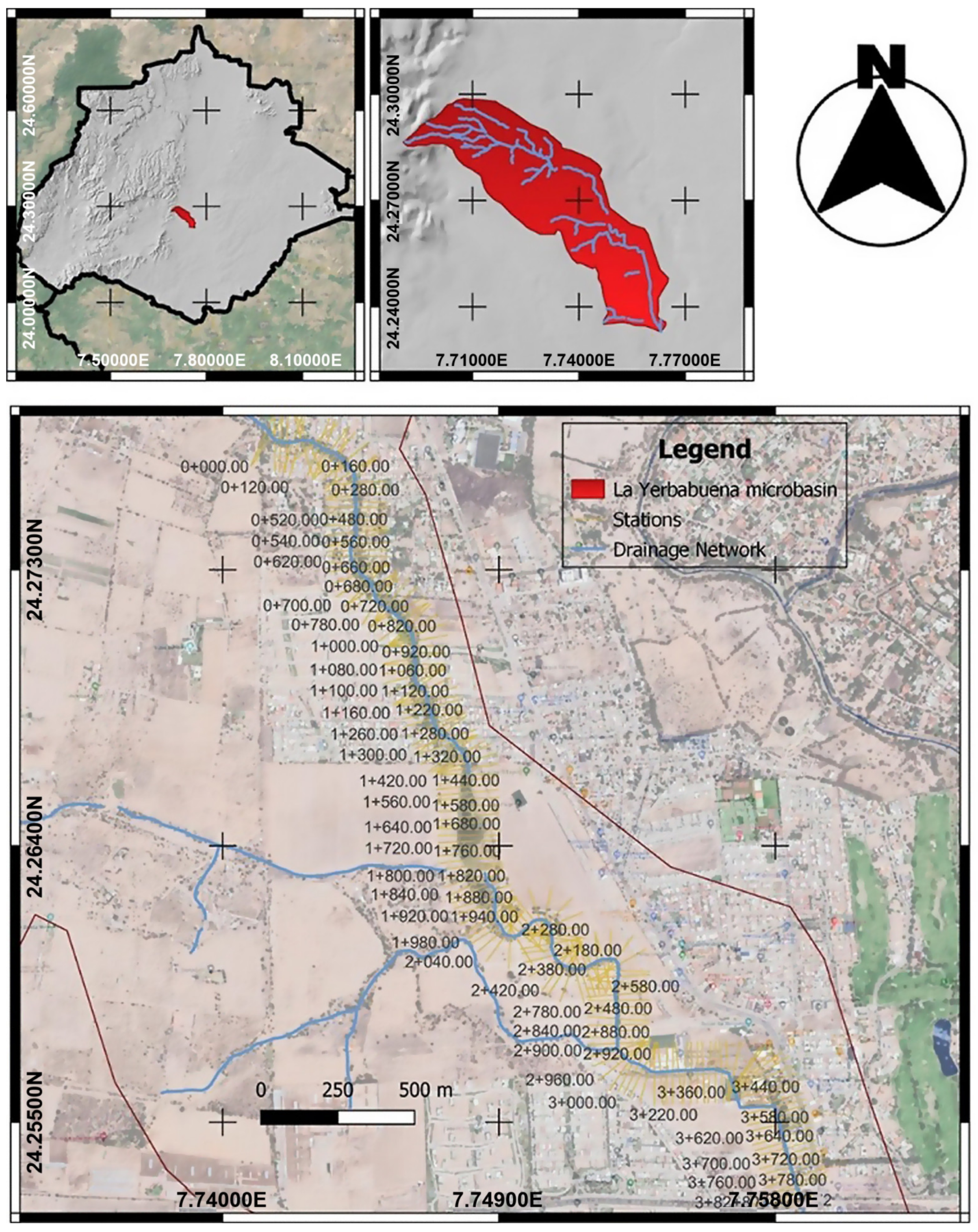
2.1. Study Area
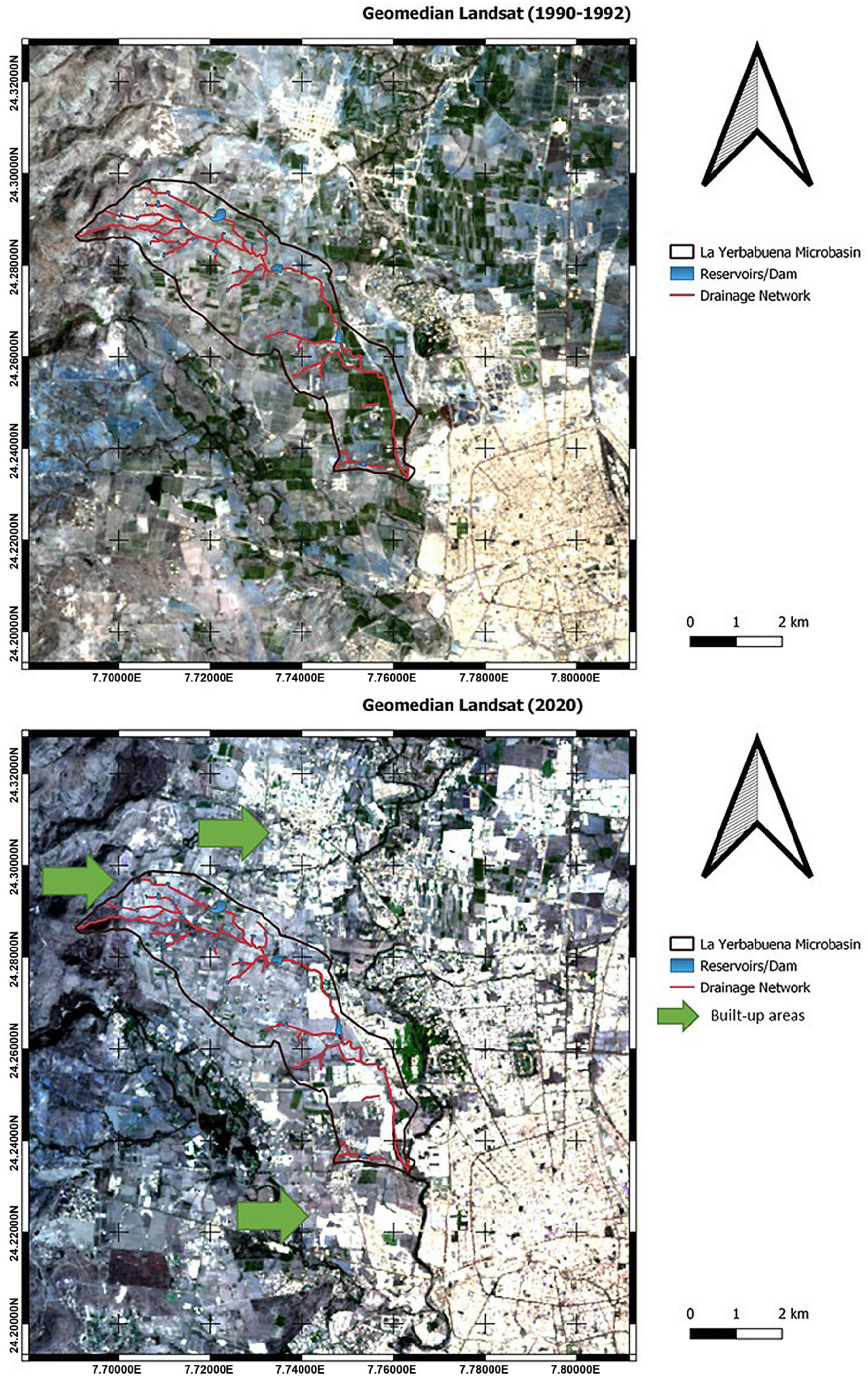
2.2. Geo-Spatial Stage
2.3. Hydrologic Stage
- Ve = Volume of runoff (m3)
- C = Runoff coefficient (adimensional)
- Pe = Excess precipitation (mm)
- A = Basin area (m2)
- P = Precipitation record (mm)
- N = Runoff curve number for the average moisture condition of the basin (adimensional)
2.4. Hydraulic Modeling Stage
2.5. Environmental Stage
3. Results
3.1. Geo-Spatial Characterization
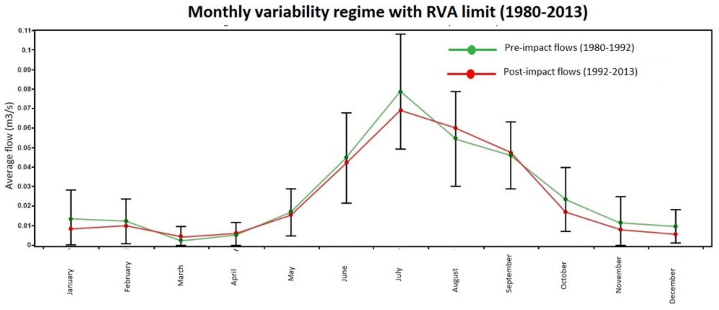
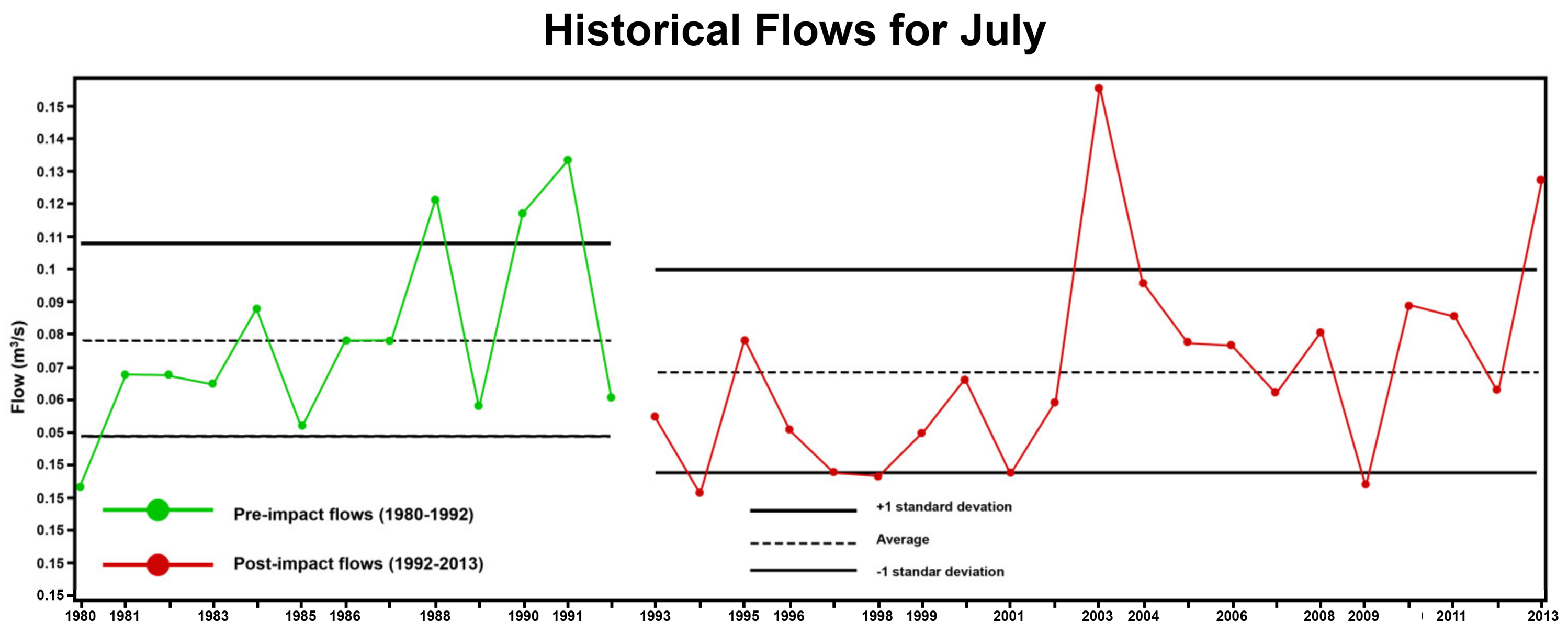
3.2. Hydrologic Characterization
3.3. Hydraulic Characterization
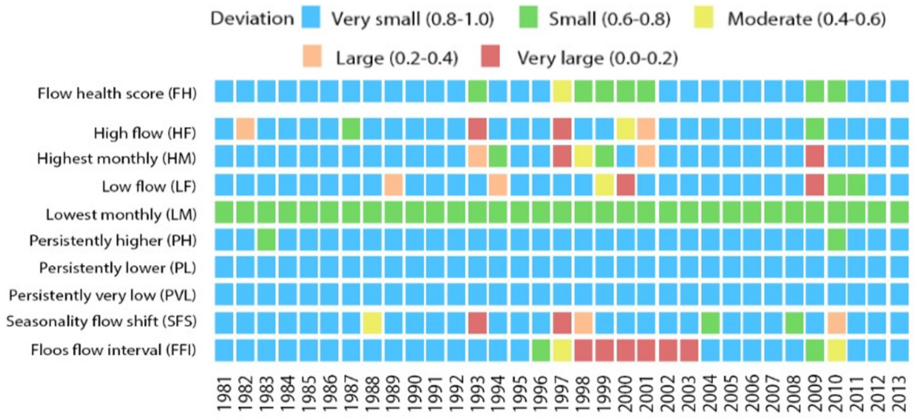
3.4. Environmental Characterization
4. Discussion
- (a)
- The extremely low flow with a frequency of 85.66%, during dry seasons, could produce the necessary conditions to form natural ponds and produce a local ecologic environment, and it could also dry low areas of flooding plains.
- (b)
- Several floods were modeled, with low frequencies between 0.64% and 0.10%.
5. Conclusions
Author Contributions
Funding
Institutional Review Board Statement
Informed Consent Statement
Data Availability Statement
Acknowledgments
Conflicts of Interest
Appendix A

| IHA Parameter Group | Hydrologic Parameters |
|---|---|
| 1. Magnitude of monthly water conditions | Mean or median value for each calendar month (subtotal 12 parameters) |
| 2. Magnitude and duration of annual extreme water conditions | Annual minima, 1-day mean annual minima, 3-day mean annual minima, 7-day mean annual minima, 30-day mean annual minima, 90-day mean annual maxima, 1-day mean annual maxima, 3-day mean annual maxima, 7-day mean annual maxima, 30-day mean annual maxima, 90-day mean number of zero-flow days, base flow index: 7-day minimum flow/mean flow for year (subtotal 12 parameters) |
| 3. Timing of annual extreme water conditions | Julian date of each annual 1-day maximum Julian date of each annual 1-day minimum (subtotal 2 parameters) |
| 4. Frequency and duration of high and low pulses | Number of low pulses within each water year. Mean or median duration of low pulses (days). Number of high pulses within each water year. Mean or median duration of high pulses (days) (subtotal 4 parameters) |
| 5. Rate and frequency of water condition changes | Rise rates: mean or median of all positive differences between consecutive daily values Fall rates: mean or median of all negative differences between consecutive daily values Number of hydrologic reversals. (subtotal 3 parameters) _________________________ Grand total: 33 parameters |
| EFC Type | Hydrologic Parameters |
|---|---|
| 1. Monthly low flows | Mean or median values of low flows during each calendar month (subtotal 12 parameters) |
| 2. Extreme low flows | Frequency of extreme low flows during each water year or season. Mean or median values of extreme low flow event: Duration (days), peak flow (minimum flow during event), timing (Julian date of peak flow) (subtotal 4 parameters) |
| 3. High flow pulses | Frequency of high flow pulses during each water year or season. Mean or median values of high flow pulse event: Duration (days), peak flow (maximum flow during event), timing (Julian date of peak flow). Rise and fall rates (subtotal 6 parameters) |
| 4. Small floods | Number of low pulses within each water year. Mean or median duration of low pulses (days). Number of high pulses within each water year. Mean or median duration of high pulses (days) (subtotal 4 parameters) |
| 5. Rate and frequency of water condition changes | Frequency of small floods during each water year or season. Mean or median values of small flood events: Duration (days), peak flow (maximum flow during event), timing (Julian date of peak flow). Rise and fall rates (subtotal 6 parameters) |
| 5. Large floods | Frequency of large floods during each water year or season. Mean or median values of large flood event: Duration (days), peak flow (maximum flow during event), timing (Julian date of peak flow). Rise and fall rates (subtotal 6 parameters) _________________________ Grand total: 34 parameters |
Appendix B
References
- Steinfeld, H.; Gerber, P.; Wassenaar, T.; Castel, V.; Rosales, M.; De Haan, C. Livestock’s Long Shadow: Environmental Issues and Options; Food & Agriculture Organization: Rome, Italy, 2006. [Google Scholar]
- Shanafield, M.; Cook, P.G. Transmission Losses, Infiltration and Groundwater Recharge through Ephemeral and Intermittent Streambeds: A Review of Applied Methods. J. Hydrol. 2014, 511, 518–529. [Google Scholar] [CrossRef]
- Alonso-Eguía-Lis, P.E.; Gómez-Balandra, M.A.; Saldaña Fabela, P. Requerimientos para Implementar el Caudal Ambiental en México; IMTA-Alianza WWF/FGRA-PHI/UNESCO-Semarnat: Jiutepec, Mexico, 2007. [Google Scholar]
- Poff, N.L.; Richter, B.D.; Arthington, A.H.; Bunn, S.E.; Naiman, R.J.; Kendy, E.; Acreman, M.; Apse, C.; Bledsoe, B.P.; Freeman, M.C.; et al. The Ecological Limits of Hydrologic Alteration (ELOHA): A New Framework for Developing Regional Environmental Flow Standards. Freshw. Biol. 2010, 55, 147–170. [Google Scholar] [CrossRef] [Green Version]
- Zhao, K.; Dong, A.; Wang, S.; Yu, X. Ecological Health Status of the Yitong River, China, Assessed with the Planktonic Index of Biotic Integrity. Water 2022, 14, 3191. [Google Scholar] [CrossRef]
- Tharme, R.E. A Global Perspective on Environmental Flow Assessment: Emerging Trends in the Development and Application of Environmental Flow Methodologies for Rivers. River Res. Appl. 2003, 19, 397–441. [Google Scholar] [CrossRef]
- González-Mora, I.; Salinas-Rodríguez, S.; Guerra Gilbert, A.; Sánchez Navarro, R.; Ríos, E. Ríos Libres y Vivos, Introducción al Caudal Ecológico y Reservas de Agua; Secretaría de Medio Ambiente y Recursos Naturales: Ciudad de México, Mexico, 2014. [Google Scholar]
- Barrios, E.; Sánchez, R.; Salinas-Rodríguez, S.; Rodriguez, J.; González, I.D.; Gomez, R.; Escobedo, H.; Reyes-González, J. Guía para la Determinación de Caudal Ecológico en México; Alianza WWF–Fundación Gonzalo Río Arronte, IAP: Mexico City, Mexico, 2011. [CrossRef]
- Mesa, D.J. Algunos Atributos de los Factores a Favor y en Contra en las Técnicas y Métodos Utilizados para la Estimación de Caudales Ambientales en Colombia. Umbral. Cient. 2009, 15, 81–93. [Google Scholar]
- Palau, A. Régimen Ambiental de Caudales: Estado del Arte; Universidad Internacional Menendez Pelayo: Madrid, Spain, 2003. [Google Scholar]
- Castro Heredia, L.M.; Carvajal Escobar, Y.; Monsalve Durango, E.A. Enfoques Teóricos Para Definir El Caudal Ambiental. Ing. Univ. 2006, 10, 1–17. [Google Scholar]
- Secretaría de Economía. NMX-AA-159-SCFI-2012; Secretaría de Economía: Mexico City, Mexico, 2012.
- Leigh, C.; Boulton, A.J.; Courtwright, J.L.; Fritz, K.; May, C.L.; Walker, R.H.; Datry, T. Ecological Research and Management of Intermittent Rivers: An Historical Review and Future Directions. Freshw. Biol. 2016, 61, 1181–1199. [Google Scholar] [CrossRef]
- Sadid, N.; Haun, S.; Wieprecht, S. An Overview of Hydro-Sedimentological Characteristics of Intermittent Rivers in Kabul Region of Kabul River Basin. Int. J. River Basin Manag. 2017, 15, 387–399. [Google Scholar] [CrossRef]
- Döll, P.; Zhang, J. Impact of Climate Change on Freshwater Ecosystems: A Global-Scale Analysis of Ecologically Relevant River Flow Alterations. Hydrol. Earth Syst. Sci. 2010, 14, 783–799. [Google Scholar] [CrossRef] [Green Version]
- Guzmán-Colis, G.; Thalasso, F.; Ramírez-López, E.M.; Rodríguez-Narciso, S.; Guerrero-Barrera, A.L.; Avelar-González, F.J. Evaluación Espacio-Temporal de La Calidad Del Agua Del Río San Pedro En El Estado de Aguascalientes, México. Rev. Int. Contam. Ambient. 2011, 27, 89–102. [Google Scholar]
- Rico-Martínez, R.; Arzate-Cárdenas, M.A.; Robles-Vargas, D.; Pérez-Legaspi, I.A.; Jesús, A.-F.; Santos-Medrano, G.E.; Rico-Martínez, R.; Arzate-Cárdenas, M.A.; Robles-Vargas, D.; Pérez-Legaspi, I.A.; et al. Rotifers as Models in Toxicity Screening of Chemicals and Environmental Samples; IntechOpen: London, UK, 2016. [Google Scholar] [CrossRef] [Green Version]
- Pacheco-Guerrero, A.; Goodrich, D.C.; González-Trinidad, J.; Júnez-Ferreira, H.E.; Bautista-Capetillo, C.F. Flooding in Ephemeral Streams: Incorporating Transmission Losses. J. Maps 2017, 13, 350–357. [Google Scholar] [CrossRef] [Green Version]
- González-Trinidad, J.; Pacheco-Guerrero, A.; Júnez-Ferreira, H.; Bautista-Capetillo, C.; Hernández-Antonio, A. Identifying Groundwater Recharge Sites through Environmental Stable Isotopes in an Alluvial Aquifer. Water 2017, 9, 569. [Google Scholar] [CrossRef] [Green Version]
- Delso, J.; Magdaleno, F.; Fernández-Yuste, J.A. Flow Patterns in Temporary Rivers: A Methodological Approach Applied to Southern Iberia. Hydrol. Sci. J. 2017, 62, 1551–1563. [Google Scholar] [CrossRef]
- The Nature Conservancy. Manual de Usuario de Indicadores de Alteración Hidrológica Versión 7.1: Nature; The Nature Conservancy: Arlington County, VA, USA, 2011. [Google Scholar]
- Palma Raymundo, M.L. Determinación del Caudal Ecológico: Impacto Económico en el Usuario Agrícola de la Cuenca Río Yautepec, Estado de Morelos, Colegio de Postgraduados (COLPOS). 2013. Available online: http://hdl.handle.net/10521/2208 (accessed on 1 February 2017).
- Bautista-de-los-Santos, Q.M. Determinación de caudales ambientales en la cuenca del río Yuna, República Dominicana. Tecnol. Cienc. Agua 2014, 5, 33–40. [Google Scholar]
- Domínguez-Sánchez, T.A.; Lomelí-Meza, J.; Ibáñez-Castillo, L.A.; Gómez-Balandra, M.A. Determinación de Caudal Ecológico del Río Mezcalapa en Base a la Norma Mexicana NMX-AA-159- SCFI-2012 Con Consideraciones Hidrológicas e Hidráulicas; Secretaría de Economía: Querétaro, Mexico, 2015. [Google Scholar]
- Li, D.; Wan, W.; Zhao, J. Optimizing Environmental Flow Operations Based on Explicit Quantification of IHA Parameters. J. Hydrol. 2018, 563, 510–522. [Google Scholar] [CrossRef]
- Richter, B.D.; Baumgartner, J.V.; Braun, D.P.; Powell, J. A Spatial Assessment of Hydrologic Alteration within a River Network. Regul. Rivers Res. Manag. 1998, 14, 329–340. [Google Scholar] [CrossRef]
- INEGI. Anuario Estadístico y Geográfico por Entidad Federativa 2015; Instituto Nacional de Estadística y Geografía: Aguascalientes, Mexico, 2015. [Google Scholar]
- Quantum Gis. Guía de Usuario QGIS; Quantum Gis: Stellenbosch/Johannesburg, South Africa, 2022. [Google Scholar]
- Campos Aranda, D.F. Introducción a la Hidrología Urbana; Printego: San Luis Potosí, Mexico, 2010. [Google Scholar]
- Martínez Martínez, S.I. Introducción a la Hidrología Superficial; Segunda: Aguascalientes, Mexico, 2011. [Google Scholar]
- Lillesand, T.; Kiefer, R.W.; Chipman, J. Remote Sensing and Image Interpretation; John Wiley & Sons: Hoboken, NJ, USA, 2014. [Google Scholar]
- Gippel, C.J.; Zhang, J.; Qu, X.; Kong, W.; Bond, N.R.; Liu, W. River Health Assessment in China: Comparison and Development of Indicators of Hydrological Health; International WaterCentre: Brisbane, Australia, 2011; Volume 195. [Google Scholar]
- García Rodríguez, E.; González Villela, R.; Martínez Austria, P.; Athala Molano, J.; Paz Soldán, G. Guía de Aplicación de los Métodos de Cálculo de Caudales de Reserva Ecológicos en México; Comisión Nacional del Agua, Subdirección General de Programación, Gerencia de Estudios para el Desarrollo Hidráulico Integral: Medellín, Columbia, 1999.


| SCS curve number | 70.00 |
| Drained area (km2) | 16.12 |
| Medium slope of the basin (m/m) | 0.02 |
| Runoff coefficient, C | 0.34 |
| Year\Month | Jan | Feb | Mar | Apr | May | Jun | Jul | Aug | Sep | Oct | Nov | Dec |
|---|---|---|---|---|---|---|---|---|---|---|---|---|
| 1979 | 0.091 | 0.005 | 0.225 | 0.278 | 0.000 | 0.000 | 0.104 | 0.966 | 0.089 | 0.147 | 0.147 | 0.135 |
| 1980 | 0.000 | 0.158 | 0.278 | 0.170 | 0.007 | 0.043 | 0.018 | 0.026 | 1.211 | 0.096 | 0.127 | 0.125 |
| 1981 | 0.011 | 0.248 | 0.294 | 0.001 | 0.259 | 0.001 | 0.000 | 0.181 | 2.648 | 0.036 | 0.127 | 0.067 |
| 1982 | 0.000 | 0.000 | 0.294 | 0.051 | 0.009 | 0.046 | 0.000 | 0.278 | 0.010 | 0.003 | 0.000 | 0.000 |
| 1983 | 0.099 | 0.000 | 0.000 | 0.000 | 0.000 | 0.874 | 0.323 | 0.002 | 0.000 | 0.072 | 0.194 | 0.000 |
| 1984 | 0.099 | 0.242 | 0.000 | 0.000 | 0.002 | 0.002 | 0.493 | 0.001 | 0.002 | 0.189 | 0.278 | 0.248 |
| 1985 | 0.263 | 0.311 | 0.000 | 0.099 | 0.087 | 0.002 | 0.046 | 0.220 | 0.038 | 0.001 | 0.317 | 0.002 |
| 1986 | 0.000 | 0.117 | 0.000 | 0.000 | 0.147 | 0.085 | 0.645 | 0.009 | 0.013 | 0.037 | 0.091 | 0.000 |
| 1988 | 0.000 | 0.000 | 0.137 | 0.147 | 0.000 | 1.504 | 0.662 | 0.005 | 0.248 | 0.000 | 0.000 | 0.000 |
| 1989 | 0.000 | 0.000 | 0.000 | 0.000 | 0.010 | 0.134 | 0.006 | 0.015 | 0.225 | 0.005 | 0.028 | 0.002 |
| 1990 | 0.091 | 0.091 | 0.000 | 0.137 | 0.117 | 0.055 | 0.807 | 0.141 | 0.005 | 0.012 | 0.000 | 0.000 |
| 1991 | 0.000 | 0.147 | 0.000 | 0.000 | 0.000 | 0.056 | 1.040 | 0.001 | 0.000 | 0.003 | 0.000 | 0.033 |
| 1992 | 0.000 | 0.170 | 0.123 | 0.091 | 0.006 | 0.280 | 0.000 | 0.259 | 0.061 | 0.111 | 0.181 | 0.186 |
| 1993 | 0.001 | 0.000 | 0.000 | 0.207 | 0.220 | 0.014 | 0.049 | 0.037 | 0.009 | 0.091 | 0.170 | 0.000 |
| 1994 | 0.001 | 0.000 | 0.000 | 0.020 | 0.127 | 0.046 | 0.037 | 0.091 | 0.015 | 0.000 | 0.000 | 0.127 |
| 1995 | 0.248 | 0.170 | 0.000 | 0.000 | 0.091 | 0.546 | 0.183 | 0.201 | 0.037 | 0.000 | 0.009 | 0.000 |
| 1996 | 0.000 | 0.294 | 0.000 | 0.263 | 0.038 | 0.014 | 0.099 | 0.005 | 0.334 | 0.000 | 0.328 | 0.000 |
| 1997 | 0.248 | 0.000 | 0.207 | 0.014 | 0.075 | 0.055 | 0.061 | 0.004 | 0.038 | 0.020 | 0.127 | 0.000 |
| 1998 | 0.000 | 0.000 | 0.000 | 0.000 | 0.000 | 0.068 | 0.051 | 0.007 | 0.003 | 0.043 | 0.000 | 0.000 |
| 1999 | 0.000 | 0.000 | 0.294 | 0.000 | 0.311 | 0.024 | 0.000 | 0.081 | 0.397 | 0.207 | 0.000 | 0.000 |
| 2000 | 0.000 | 0.000 | 0.000 | 0.000 | 0.001 | 0.000 | 0.037 | 0.005 | 0.001 | 0.220 | 0.000 | 0.049 |
| 2001 | 0.000 | 0.194 | 0.003 | 0.083 | 0.248 | 0.001 | 0.006 | 0.014 | 0.021 | 0.049 | 0.294 | 0.335 |
| 2002 | 0.061 | 0.061 | 0.000 | 0.000 | 0.014 | 0.546 | 0.056 | 0.546 | 0.021 | 0.091 | 0.037 | 0.000 |
| 2003 | 0.248 | 0.311 | 0.000 | 0.000 | 0.028 | 0.442 | 1.668 | 0.003 | 0.009 | 0.091 | 0.000 | 0.000 |
| 2004 | 0.000 | 0.000 | 0.091 | 0.000 | 0.002 | 0.417 | 0.323 | 0.718 | 0.021 | 0.234 | 0.294 | 0.000 |
| 2005 | 0.000 | 0.003 | 0.127 | 0.000 | 0.091 | 0.779 | 0.119 | 0.417 | 0.020 | 0.220 | 0.000 | 0.248 |
| 2006 | 0.248 | 0.000 | 0.000 | 0.000 | 0.091 | 0.006 | 0.442 | 0.005 | 0.020 | 0.323 | 0.000 | 0.005 |
| 2007 | 0.061 | 0.061 | 0.000 | 0.028 | 0.002 | 0.261 | 0.183 | 0.033 | 0.000 | 0.108 | 0.311 | 0.311 |
| 2008 | 0.000 | 0.000 | 0.000 | 0.068 | 0.311 | 0.004 | 0.085 | 0.166 | 0.021 | 0.000 | 0.000 | 0.000 |
| 2009 | 0.000 | 0.000 | 0.000 | 0.000 | 0.248 | 0.055 | 0.041 | 0.078 | 0.003 | 0.004 | 0.038 | 0.117 |
| 2010 | 0.017 | 0.442 | 0.000 | 0.263 | 0.278 | 0.009 | 0.001 | 0.006 | 0.000 | 0.000 | 0.000 | 0.000 |
| 2011 | 0.000 | 0.000 | 0.000 | 0.311 | 0.000 | 0.005 | 0.127 | 0.099 | 0.005 | 0.075 | 0.000 | 0.000 |
| 2012 | 0.075 | 0.009 | 0.000 | 0.000 | 0.000 | 0.067 | 0.032 | 0.072 | 0.104 | 0.127 | 0.294 | 0.006 |
| 2013 | 0.147 | 0.000 | 0.000 | 0.000 | 0.000 | 0.091 | 0.826 | 0.002 | 0.012 | 0.028 | 0.002 | 0.000 |
| Y/M | Jan | Feb | Mar | Apr | May | Jun | Jul | Aug | Sep | Oct | Nov | Dec |
|---|---|---|---|---|---|---|---|---|---|---|---|---|
| Dry | 0.000 | 0.000 | 0.000 | 0.000 | 0.000 | 0.000 | 0.000 | 0.000 | 0.003 | 0.000 | 0.000 | 0.000 |
| Humid | 0.263 | 0.442 | 0.294 | 0.311 | 0.311 | 1.504 | 1.668 | 0.966 | 2.648 | 0.323 | 0.328 | 0.335 |
| Average | 0.059 | 0.089 | 0.061 | 0.066 | 0.083 | 0.192 | 0.252 | 0.138 | 0.166 | 0.078 | 0.100 | 0.059 |
| Genera—Species | Local Name |
|---|---|
| Acacia farnesiana | Huizache |
| Yucca filifera Chabaud | Palma (palm) |
| Prosopis glandulosa | Mezquite |
| Ferocactus wislizenii | Biznaga (barrel cactus) |
| Gomphrena serrata L. | Betónica, Bolas de hilo, Borreguilla, Betónica, Cabeza de indio, Escobetilla |
| Dysphania graveolens_(Wild.) Mosyakin & Clements | Epazote de zorrillo (skunk epazote) |
| Gnaphalium spp. | Gordolobo (mullein) |
| Zinnia Angustifolia kunth | Hierba de la pastora, Pastora (shepherd grass) |
| Bidens odorata Cav. | Aceitilla, Aceitilla blanca (White aceitilla) |
| Grindelia oxylepis Greene | Árnica amarilla (yellow arnica) |
| Heterotheca inuloides Cass. var. rosei Wagenkn. | Árnica amarilla (yellow arnica) |
| Aster gymnocephalus (DC.) | Árnica morada (purple arnica) |
| Tagetes lunulata Ort. | Cinco llagas, Flor de cinco llagas (five-blisters flower) |
| Zinnia peruviana (L.) L. | Mal de ojo (evil eye) |
| Sanvitalia procumbens Lam. | Ojo de gato (cat eye) |
| Tithonia Desf. ex Juss. | Titonia |
| Cardenche Opuntia imbricata (Haw.) DC. | Cardenche |
| Opuntia streptacantha Lemaire | Nopal cardón |
| Opuntia jaliscana Bravo | Nopal chamacuero |
| Opuntia leucotricha De Candolle | Xoconostle amarillo, Duraznillo (Yellow xoconostle) |
| Ipmoea murucoides | palo bobo (silly stick) |
| Ipomoea purpurea (L.) Roth | Hiedra de flores chiquitas (tiny-flowers ivy) |
| Lepidium virginicum L. | Chile de pájaro (bird chilli) |
| Cucurbita foetidissima Kunth | Calabacilla loca (crazy zucchini) |
| Ricinus comunis | Higuerilla |
| Mimosa monancistra | Gatuño |
| Yucca filifera | Izotal |
| Genera—Species | Local name |
|---|---|
| Zenaida asiática | Paloma aliblanca (white-winged dove) |
| Anas platyrhynchos | Pato mexicano (Mexican duck) |
| Charadrius vociferus | Tildio |
| Hirundo rustica | Golondrina (swallow) |
| Anolis nebolosus | Culebra de agua (water snake) |
| Spea multiplicatus | Sapo (toad) |
| Rana montezumae | Rana común (common frog) |
| Kinosternum integrum | Tortuga terrestre (land turtle) |
| Month | Average Year Qaa | Appendix C Qe (NMX-159) | Appendix D Qe (NMX-159) | IHAQe |
|---|---|---|---|---|
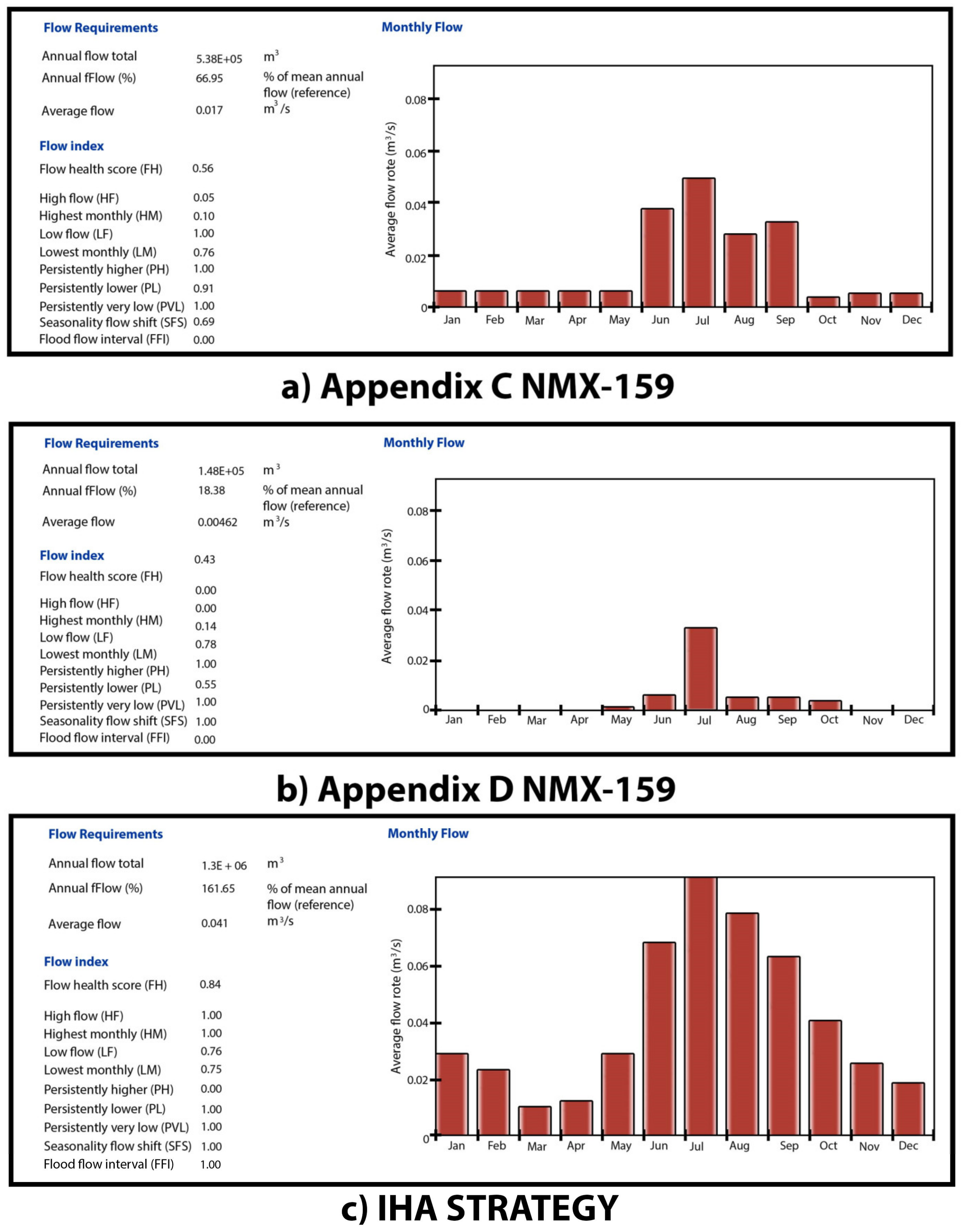
| Jan | 0.059 | 0.006 | 0.000 | 0.028 |
| Feb | 0.089 | 0.006 | 0.000 | 0.024 |
| Mar | 0.061 | 0.006 | 0.000 | 0.010 |
| Apr | 0.066 | 0.006 | 0.000 | 0.012 |
| May | 0.083 | 0.006 | 0.001 | 0.029 |
| Jun | 0.192 | 0.038 | 0.006 | 0.068 |
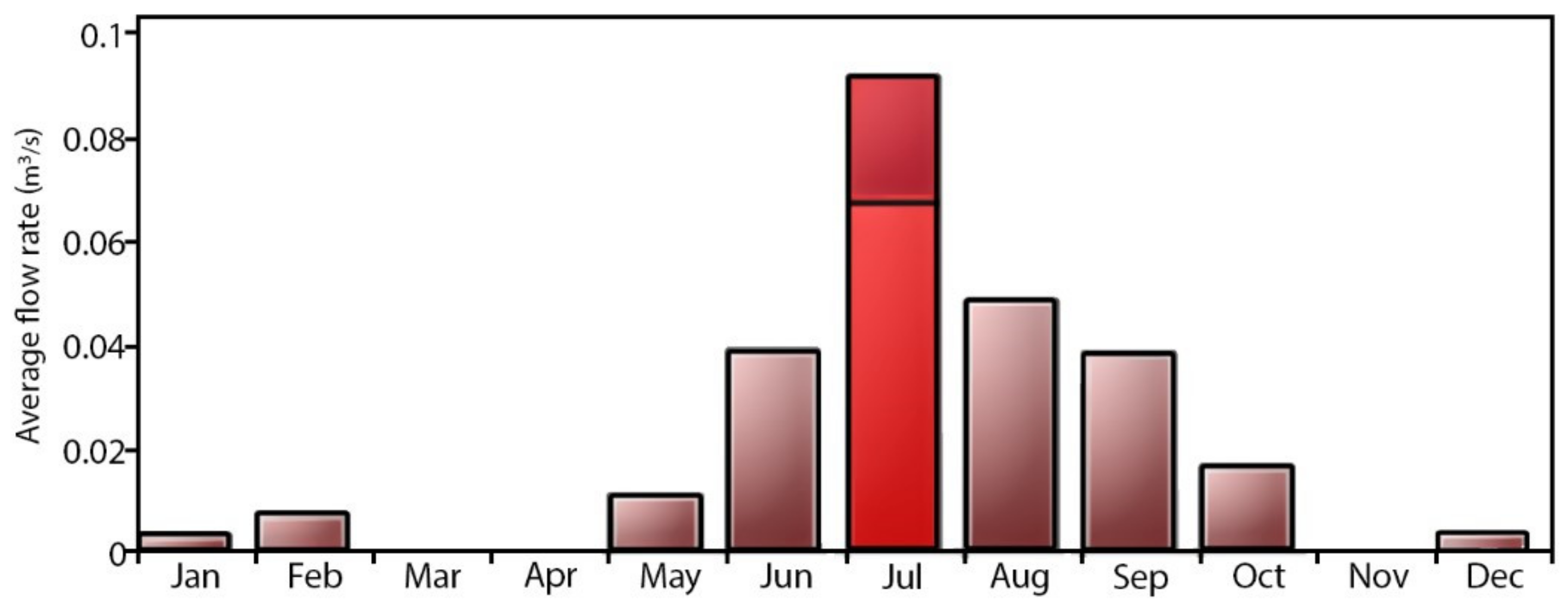
| Jul | 0.252 | 0.050 | 0.032 | 0.108 |
| Aug | 0.138 | 0.028 | 0.005 | 0.079 |
| Sep | 0.166 | 0.033 | 0.005 | 0.063 |
| Oct | 0.078 | 0.006 | 0.003 | 0.040 |
| Nov | 0.100 | 0.006 | 0.000 | 0.025 |
| Dec | 0.059 | 0.006 | 0.000 | 0.018 |
| Parameter | Hydrologic Methodologies | ||
|---|---|---|---|
| IHA | Appendix C (NMX-159) | Appendix D (NMX-159) | |
| Hydrologic Stage | |||
| Hydro/average environmental flow, m3/s | 0.042 | 0.016 | 0.004 |
| Minimum value in dry seasons, m3/s | 0.01 | 0.006 | 0.000 |
| Maximum value in rain seasons, m3/s | 0.108 | 0.050 | 0.032 |
| Pre-impact dry period, days | 320 | ||
| Post-impact dry period, days | 330 | ||
| Other features | Environmental flow components of low flow and extremely low flow. | ||
| Hydraulic Stage | |||
| Maximum levels of water, m | 0.1 to 0.2 | 0.06 to 0.13 | 0.14 only in rain season |
| Environmental Stage | |||
| Flow Health score | 0.84 | 0.56 | 0.43 |
| Remaining flow for neighboring fauna, m3/s | 0.037 | 0.013 | 0.001 |
Disclaimer/Publisher’s Note: The statements, opinions and data contained in all publications are solely those of the individual author(s) and contributor(s) and not of MDPI and/or the editor(s). MDPI and/or the editor(s) disclaim responsibility for any injury to people or property resulting from any ideas, methods, instructions or products referred to in the content. |
© 2023 by the authors. Licensee MDPI, Basel, Switzerland. This article is an open access article distributed under the terms and conditions of the Creative Commons Attribution (CC BY) license (https://creativecommons.org/licenses/by/4.0/).
Share and Cite
Reyes-Cedeño, I.G.; Hernández-Marín, M.; Pacheco-Guerrero, A.I.; Gannon, J.P. Comprehensive Methodology and Analysis to Determine the Environmental Flow Regime in the Temporary Stream “La Yerbabuena” in Aguascalientes, Mexico. Water 2023, 15, 879. https://doi.org/10.3390/w15050879
Reyes-Cedeño IG, Hernández-Marín M, Pacheco-Guerrero AI, Gannon JP. Comprehensive Methodology and Analysis to Determine the Environmental Flow Regime in the Temporary Stream “La Yerbabuena” in Aguascalientes, Mexico. Water. 2023; 15(5):879. https://doi.org/10.3390/w15050879
Chicago/Turabian StyleReyes-Cedeño, Isaí Gerardo, Martín Hernández-Marín, Anuard Isaac Pacheco-Guerrero, and John P. Gannon. 2023. "Comprehensive Methodology and Analysis to Determine the Environmental Flow Regime in the Temporary Stream “La Yerbabuena” in Aguascalientes, Mexico" Water 15, no. 5: 879. https://doi.org/10.3390/w15050879