Article

Detection of Water Hyacinth (Eichhornia crassipes) in Lake Tana, Ethiopia, Using Machine Learning Algorithms

1
Graduate School of Science and Engineering, Soka University, Hachioji, Tokyo 192-8577, Japan
2
College of Agriculture and Environmental Science, Bahir Dar University, Bahir Dar 6000, Ethiopia
3
Lake Biwa Environmental Research Institute, Otsu 520-0022, Japan
*
Author to whom correspondence should be addressed.
Water 2023, 15(5), 880; https://doi.org/10.3390/w15050880
Submission received: 24 November 2022 / Revised: 29 January 2023 / Accepted: 2 February 2023 / Published: 24 February 2023

Abstract

:
Lake Tana is Ethiopia’s largest lake and is infested with invasive water hyacinth (E. crassipes), which endangers the lake’s biodiversity and habitat. Using appropriate remote sensing detection methods and determining the seasonal distribution of the weed is important for decision-making, water resource management, and environmental protection. As the demand for the reliable estimation of E. crassipes mapping from satellite data grows, comparing the performance of different machine learning algorithms could help in identifying the most effective method for E. crassipes detection in the lake. Therefore, this study aimed to examine the ability of random forest (RF), support vector machine (SVM), and classification and regression tree (CART) machine learning algorithms to detect E. crassipes and estimating seasonal spatial coverage of the weed on the Google Earth Engine (GEE) platform using Landsat 8 and Sentinel 2 images. Cloud-masked monthly median composite Landsat 8 and Sentinel 2 data from October 2021 and 2022, January 2022 and 2023, March 2022, and June 2022 were used to represent autumn, winter, spring, and summer, respectively. Four spectral indices were derived and used in combination with spectral bands to improve the E. crassipes detection accuracy. All methods achieved greater than 95% and 90% overall accuracy when using Sentinel 2 and Landsat 8 images, respectively. Using both data sets, all methods achieved a greater than 93% F1 score for E. crassipes detection. Though the difference in performance between the methods was small, the RF was the most accurate, while the SVM and CART methods had the same accuracy. The maximum E. crassipes coverage area was observed in autumn (22.4 km2), while the minimum (2.2 km2) was observed in summer. Based on Sentinel 2 data, the E. crassipes area coverage decreased significantly by 62.5% from winter to spring and increased significantly by 81.7% from summer to autumn. The findings suggested that the RF classifier was the most accurate E. crassipes detection algorithm, and autumn was an appropriate season for E. crassipes detection in Lake Tana.

1. Introduction

Lake Tana is the largest highland lake in Ethiopia and holds ecological, religious, historical, and economic significance [1]. The lake accounts for approximately 33% of the total volume of inland water resources and 52% of the total water surface area of the country [2]. However, the lake is currently infested with a rapidly reproducing herbaceous water hyacinth (Eichhornia Crassipes) weed, which is one of the most invasive weeds in the world [3,4]. The plant is known for causing significant social, economic, and ecological harm in tropical and subtropical climates worldwide [5,6]. In particular, its proliferation reduces biodiversity, affects regional habitats, reduces water quality and fish production, harms native aquatic plant species, and impacts hydroelectric power generation by reducing the lake’s water storage capacity [7,8,9,10,11,12,13,14]. Further, the invasive weeds have a significant impact on the lives of local communities whose livelihoods are heavily reliant on the lake by blocking waterways, clogging irrigation channels, impairing fishing and transportation, and hindering tourism [15,16,17,18,19,20,21,22]. The first presence of water hyacinth in Lake Tana was recognized in 2011 [23] and has continued to expand at an alarming rate. The total shoreline length of Lake Tana is estimated to be 385 km with over 30% now infested with E. crassipes. However, the extent of the infestation varies along the shoreline and changes with seasons. Understanding the spatial distribution and growth patterns of the weed during different seasons is crucial for developing effective mitigation measures.
Remote sensing satellites are used to determine the spatial and temporal distribution of ground objects [24,25,26]. Satellite data have the potential to provide effective, low-cost, and short-interval monitoring of the spatial and temporal distribution of E. crassipes infestations on large scales [5]. Machine learning algorithms are increasingly being used to classify and detect ground objects from satellite images due to their high efficiency and accuracy when compared with common parametric algorithms, such as maximum likelihood classifiers (MLCs) [27,28,29,30,31,32,33,34,35]. When identifying the distribution of E. crassipes from satellite imagery, machine learning algorithms have the potential to significantly improve detection accuracy, enhance clean-up efforts, and forecast potential hotspots [5]. Among the machine learning algorithms, random forest (RF), classification and regression tree (CART), and support vector machine (SVM) algorithms are widely used for remote sensing image analysis due to their classification accuracy [36]. RF and SVM algorithms are known for their robustness and accuracy in image classification tasks, and the ability to handle high-dimensional data [37,38]; the CART algorithm is known for its interpretability and simplicity [39]. Additionally, deep learning techniques, such as convolutional neural networks (CNNs), are also commonly used for image classification tasks and have shown promising results. However, they are computationally more expensive than common machine learning methods [40]. There is no single machine learning algorithm that can handle all pattern recognition tasks due to differences in texture and spectral reflectance of the ground features, and different algorithms often produce variable results [31]. Moreover, the relative performance of various classification methods will vary by season due to changes in the physiological characteristics of plants and the life cycle influence on spectral reflectance.
Previous studies utilized different classifiers, such as the maximum likelihood classifier (MLC) [1,14,19], decision tree [19], and random forest (RF) [41], to determine the spatial and temporal distribution of E. crassipes in Lake Tana. However, most studies on Lake Tana focused only on the northeastern part and used Level 1 top-of-atmosphere (TOA) satellite imagery without any atmospheric correction and only used spectral bands. For example, Dersseh et al. [41] used the RF method to classify and estimate the areal cover of E. crassipes from Sentinel-2 MSI Level-1C TOA data but focused within the lake shoreline boundary without atmospheric corrections. Similarly, Worqlul et al. [1] used the MLC method on PlanetScope Level 1 top-of-atmosphere (TOA) products without considering atmospheric correlations in their analysis. However, atmospheric corrections are crucial for accurately estimating the coverage area and spatiotemporal patterns of aquatic plants in lake environments [26,42]. Furthermore, Asmare et al. [19] employed a decision tree algorithm for E. crassipes detection in Landsat 8 images but did not evaluate the classifier’s accuracy; however, accuracy is crucial for evaluating the performance of a classifier. To our knowledge, no comparative studies evaluated the effectiveness of different machine learning algorithms for E. crassipes detection during different seasons in Lake Tana. Given the unique characteristics of the lake and the species, certain algorithms may perform better under different conditions. Conducting a study that compares the performance of various algorithms for E. crassipes detection will help to identify the most effective approach for detecting the weed in the lake. Further, the conditions and distribution of E. crassipes in the lake may have evolved since previous studies, and there may be a need to update the information on the lake’s current status.
The spectral reflectance of E. crassipes varies with age and season, and the most suitable machine learning algorithm for detection during different seasons must be clarified. Non-parametric machine learning methods, such as random forests (RFs), classification and regression trees (CARTs), and support vector machines (SVMs), can effectively handle outliers in training data [43] and often perform better on complex and non-linear datasets. The purpose of this study was to compare the performance of three non-parametric machine learning algorithms (RF, SVM, and CART) for detecting E. crassipes, and quantify spatial coverage using atmospherically corrected Sentinel 2 and Landsat 8 images spectral bands and indices in combination using the Google Earth Engine (GEE) platform during different seasons. Comparing the performance, identifying the most efficient machine-learning method, and quantifying the spatial coverage of E. crassipes using the most accurate method will provide a more complete understanding of the seasonal variability and spatial coverage of the infestation, inform management and control strategies, and improve decision-making by providing accurate and up-to-date information on the E. crassipes infestation.

2. Materials and Methods

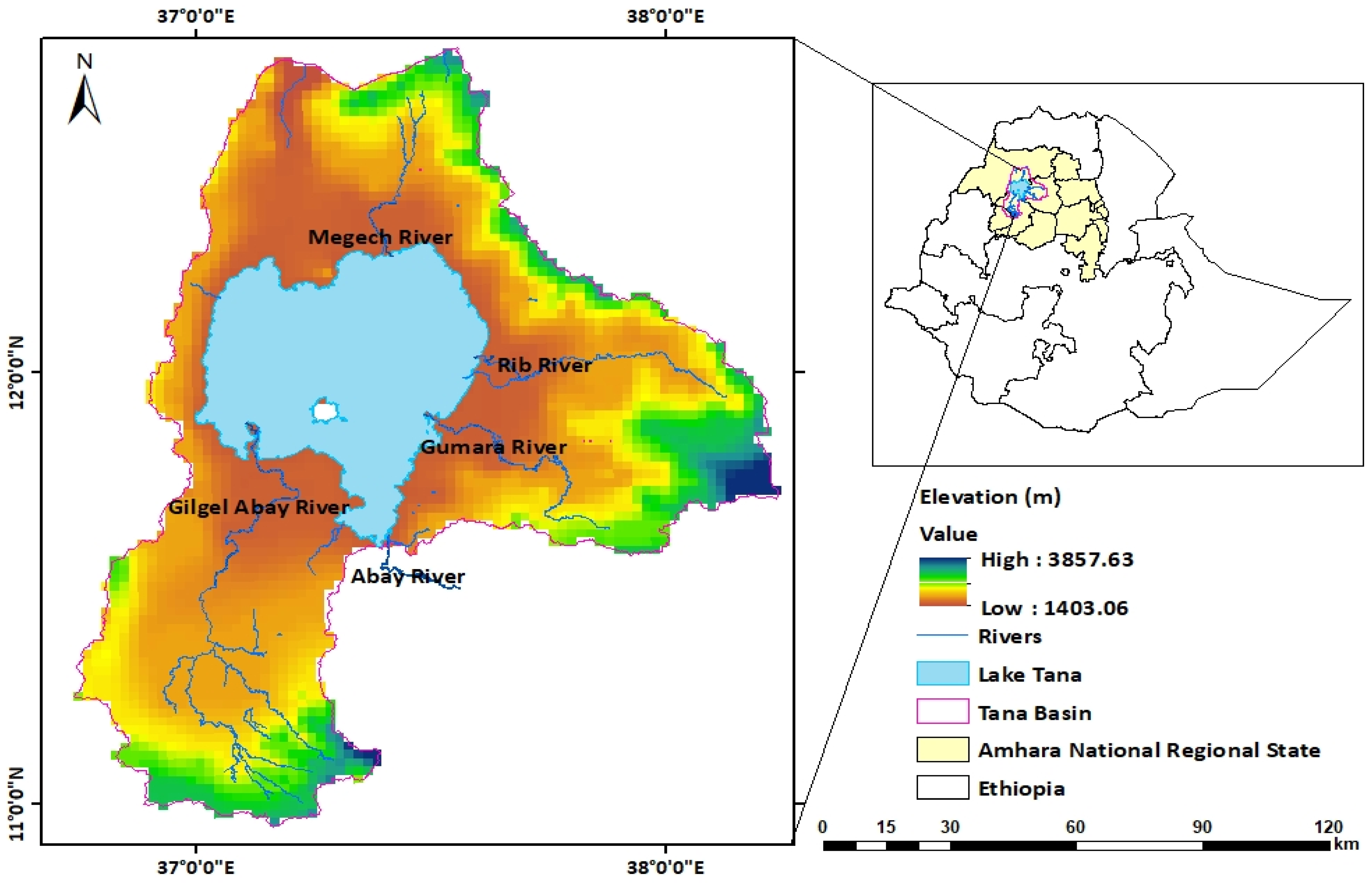
2.1. Description of the Study Area

Lake Tana is situated in northwest Ethiopia (Figure 1) and is the source of the Abay River (Blue Nile River outside Ethiopia), with an average elevation of about 1786 m above sea level [44]. It is the largest highland lake in Ethiopia, and its surface water area varies from 2966 to about 3100 km2 depending on the seasonal fluctuations in lake levels [45]. The lake receives 95% of its inflow from four major rivers, namely, the Megech, Rib, Gumara, and Gilgel Abay Rivers [46]. The regional climate is divided into four seasons: summer (Kiremt, the main rainy season) from June to August, autumn (Tseday, the post-rainy season) from September to November, winter (Bega, the dry season) from December to February, and spring (Belg, the minor rainy season) from March to May [47,48]. Precipitation is highest in July and August (250–330 mm per month), and the annual mean rainfall is about 1280 mm [16]. The air temperature has high daily variability, but the seasonal variability is relatively low, with an annual mean temperature of 20 °C [49]. The present study was conducted within and around the shoreline of Lake Tana with a 2 km buffer zone extending outward from the shoreline.

2.2. Data Types and Pre-Processing

In this study, atmospherically corrected Level 2A processed Sentinel 2 multispectral instrument (MSI) and Level 2 Landsat 8 operational land imager (OLI) Tier 1 surface reflectance data were used. The cloud mask algorithm, which is available on the GEE platform, was used to remove unclear pixels caused by cloud contamination from all available images. Median temporal composite methods were used to fill gaps in cloudy images. The monthly median composite of Landsat 8 and Sentinel 2 images acquired in October 2021, January 2022, March 2022, and June 2022 were used to represent autumn, winter, spring, and summer, respectively. A monthly median composite of Sentinel 2 images from October 2022 and a twenty-day median composite of Sentinel 2 images from January 2023 were also used for comparison and to quantify the E. crassipes spatial coverage during autumn (2022) and winter (2023), respectively. Imagery with less than five percent (<5%) cloud cover was used for autumn, winter, and spring. Due to high cloud contamination during summer (the rainy season), it was difficult to obtain images with <5% cloud cover, and only images with <10% cloud cover were available in June. Thus, images acquired in June 2022 were used to represent summer. Landsat 8 data bands two through seven (B2–B7) at a 30 m resolution and Sentinel 2 data comprising four bands at a 10 m resolution and six bands at a 20 m resolution were used in this study (Table 1). However, Sentinel 2 bands at a 10 m resolution were downscaled to a 20 m resolution using a resampling algorithm in JavaScript on the GEE platform to improve the overall detection accuracy by balancing spatial resolution and computational efficiency.
In addition to the raw spectral bands presented in Table 1, classifiers were provided with four derived environmental indices of water and vegetation. Nine spectral indices, namely, the normalized difference vegetation index (NDVI), enhanced vegetation index (EVI), chlorophyll index green (Clg), normalized difference water index (NDWI), simple ratio index (SRI), modified normalized difference water index (MNDWI), green normalized difference vegetation index (GNDVI), optimized soil adjusted vegetation index (OSAVI), and difference vegetation index (DVI), were generated. In order to identify less correlated indices, a pairwise correlation between the bands and indices was calculated using the ee.Reducer.pearsonsCorrelation() function in the GEE. Five indices (GNDVI, OSAVI, DVI, EVI, and Clg) were identified as being correlated to each other and were removed. The remaining four indices (NDVI, SRI, NDWI, and MNDWI) (Table 2) were less correlated and used as inputs for the classifier, along with the spectral bands to improve the E. crassipes detection accuracy.

2.3. Sample Point Generation Methods

Images were classified into four land-use/cover classes: water (clear and turbid), water hyacinth (E. crassipes), other vegetation, and bare land. Other vegetation classes included all vegetation types, such as crops, wetlands, grazing lands, and forests. Bare land included sediment deposition areas, cultivated land without crops, buildings, and rock outcrops. In situ field data and visual interpretation of multi-temporal Landsat 8 and Sentinel 2 images with the help of high-resolution Google Earth images, field knowledge, and expert opinions were used to manually digitize the four land-use/cover classes. A handheld global positioning system (GPS) (GARMIN 72) was used to collect field data on the E. crassipes patches in Lake Tana. In addition to field data, the study used visual interpretation of multi-temporal images to collect sample points with the help of Google Earth high-resolution images as follows: (1) different sample points were selected from Landsat 8 and Sentinel 2 images based on field knowledge, previous studies, and reports of Lake Tana, and (2) the sample points were exported to the Keyhole Markup Language (KML) format and then imported into Google Earth Pro to check the reliability and validity of the sample points using high-resolution Google Earth images.
Irregular polygons were defined from the four land-use/cover classes in the March 2022 image using both GPS points and sample points collected through visual interpretation of Landsat 8 and Sentinel 2 images. Similarly, irregular polygons from the four land-use/cover classes were defined in October 2021 and 2022, January 2022 and 2023, and June 2022 based on sample points collected through the visual interpretation of images. Stratified random sampling was carried out after irregular polygon land-use/cover delineations within each of these polygons. However, land-use/cover polygons were distributed evenly across the study area to define strata. Image classification is affected by the number and distribution of training samples. Since the classifier parameter suffers from missing or unbalanced training samples, the stratified sampling method developed using the GEE can extract the same number of samples from each class and can avoid over- and under-fitting [54]. According to the rule of thumb, each class requires a minimum of 50 training data points for classification [55]. The stratified sampling method ensures the selection of samples from all available classes and was used to generate 1200 labeled samples (300 for each class), with 70% used for training and the remainder used for validation.
Three non-parametric machine learning methods available in the GEE platform were used and chosen for their ability to handle outliers in the training data. A detailed explanation of each classifier and process is given below.
Classification and regression tree (CART): A CART is a binary decision classification tree [39]. The algorithm enables simple decision-making in logical if–then scenarios. It recursively divides the feature space into smaller regions, or nodes, based on the values of one or more input features by selecting the feature and the threshold value that will produce the most “pure” child nodes. A CART is simple to interpret and understand but is heavily influenced by the sample size employed for each class. Its effectiveness is also hindered by high-dimensionality data, which results in complex tree architectures [36]. A CART can be prone to overfitting, especially when the tree is deep and complex. To deal with overfitting, the data tree can be pruned by setting a minimum number of observations per leaf. In this study, a cross-validation technique was used to determine the optimal number of observations per leaf, and a value of 10 produced high accuracy, resulting in the minimum number of observations per leaf being set to 10. The ee.Classifier.smileCart() function is part of the Google Earth Engine (GEE) JavaScript API and creates a CART classifier. The ee.Classifier.smileCart() function was used to train the CART classifier with a given set of training data and feature bands. The classify() function was used to apply the trained classifier to the target imagery to classify each pixel of the image into one of the predefined classes.
Random forest (RF): The RF method was first introduced by Breiman [43]. An RF is an ensemble machine learning method that uses multiple CART trees to make predictions. In an RF, multiple trees are created by selecting a random subset of the data, which are then combined to give a more accurate and stable prediction [43]. Because of the randomness of the sample and feature selection, an RF has the advantages of strong noise resistance, generalization ability, and strong processing ability for high-dimensional data without the need to manually select features [37]. A number of trees in the 50–500 range performed better with higher accuracy for RF classification. In the present study, 300 trees produced good results, and thus, the number of trees was set to 300 for all datasets. The ee.Classifier.smileRandomForest() function is part of the GEE JavaScript application programming interface (API) and creates an RF classifier. The function ee.Classifier.smileRandomForest() was used to train the RF classifier, and then the classify() function was used to apply the trained classifier to the target imagery.
Support vector machine (SVM): An SVM is a supervised classification algorithm that formulates a classification function based on an optimal hyperplane to separate classes using training data based on the process that is performed [56]. An SVM can help to determine the locality of decision boundaries or hyperplanes between classes or land-cover types [38,57]. It is a binary classifier that can assess pixels from known training samples into one or two possible classes, where the distance of each class from the data points in the training data to the optimal hyperplane is maximized [58,59]. This method helps to reduce the misclassifications that occur during training [60]. The most representative samples could be obtained by finding a hyperplane between classes. The cost parameter (C), gamma, and kernel functions are the most important parameters for selecting support vectors [36]. A grid search technique was used to determine the optimal values for the C and linear kernel in this method. The C has a significant impact on SVM performance and support vector selection. The linear kernel is recommended for large datasets because it is computationally efficient and can handle high-dimensional data [61]. For the SVM classification, the C-SVC method with a cost parameter of 10 and a linear kernel type was used. The function ee.Classifier.libsvm() was used to create a support vector machine (SVM) classifier in the Google Earth Engine (GEE) JavaScript API. The ee.Classifier.libsvm() function is a wrapper for the LIBSVM library, which is a widely used library for SVM classification and regression. The function ee.Classifier.svm() was used to train the SVM classifier, and then the classify() function was used to apply the trained classifier to the target imagery.

2.4. Accuracy Assessment

This study used an accurate validation sample set that was independent of the training sample sets to evaluate the accuracy of the classified images. Validation samples were distributed using equal-area stratified random sampling, which ensured that the validation samples were uniformly distributed globally and randomly distributed locally [62]. The classified images produced using the RF, SVM, and CART algorithms on Landsat 8 and Sentinel 2 images were tested in the form of a confusion matrix by comparing the true class with the classes assigned by the classifiers using JavaScript in GEE. The machine learning classifier performance was evaluated by comparing the accuracy of the classified images with the most commonly used quality metrics, such as the overall accuracy (OA) (Equation (1)) [63] and the kappa coefficient (K) (Equation (2)) [36].
OA = Number   of   Correctly   Classified   Samples Number   of   Total   Samples × 100
The overall accuracy is a measure of how well a reference sample is classified by comparing the number of correctly classified samples to the total number of samples. It gives a percentage of the reference sites that were correctly mapped out from the entire data set [64].
K = N   1 = 1 r X i i 1 = 1 r ( X i + ×   X + i ) N 2 1 = 1 r ( X i + ×   X + i )  
The kappa coefficient (K) is determined using Equation (2), where r represents the number of rows and columns in the error matrix, Xii represents the number of observations in row i and column i, Xi + represents the marginal total of row i, X + i represents the marginal total of column i, and N represents the total number of observations. The kappa coefficient measures the degree to which the accuracy in a classification system exceeds what would be achieved by random chance.
Furthermore, the user accuracy (UA; Equation (3)), producer’s accuracy (PA; Equation (4)), and F1 score (Equation (5)) at the class level were used [63].
UA = Number   of   Correctly   Classified   Samples   in   each   class Number   of   Samples   Classified   to   that   class    
PA = Number   of   Correctly   Classified   Samples   in   each   class Number   of   Samples   from   Reference   Data   in   each   Class    
F 1 = 2 × UA × PA UA + PA  
The F1 score is the harmonic mean of producer and user accuracies and can be used to assess accuracy at the class level [65]. The F1 score is the best performance metric and is widely used, giving equal importance to both the PA and UA by combining them into a single model performance metric [63,66,67].
The spatial coverage (area) of E. crassipes and other land-use/cover in the study region was calculated using the grouped reducer and reduceRegion() function on the Google Earth Engine (GEE) platform and the result was exported as a table for further analysis. Moreover, spectral reflectance curves of Sentinel 2 images were used to determine the best bands for distinguishing E. crassipes from other land-use/cover types. Moreover, the feature importance of the RF classifier was assessed using the explain() method in the GEE for different seasons in Sentinel 2 images to evaluate the influence of spectral bands and indices on the classifier’s accuracy. Feature importance values indicate how much each input feature, such as spectral bands or indices, contributed to the predictions made by the RF classifier.

3. Results

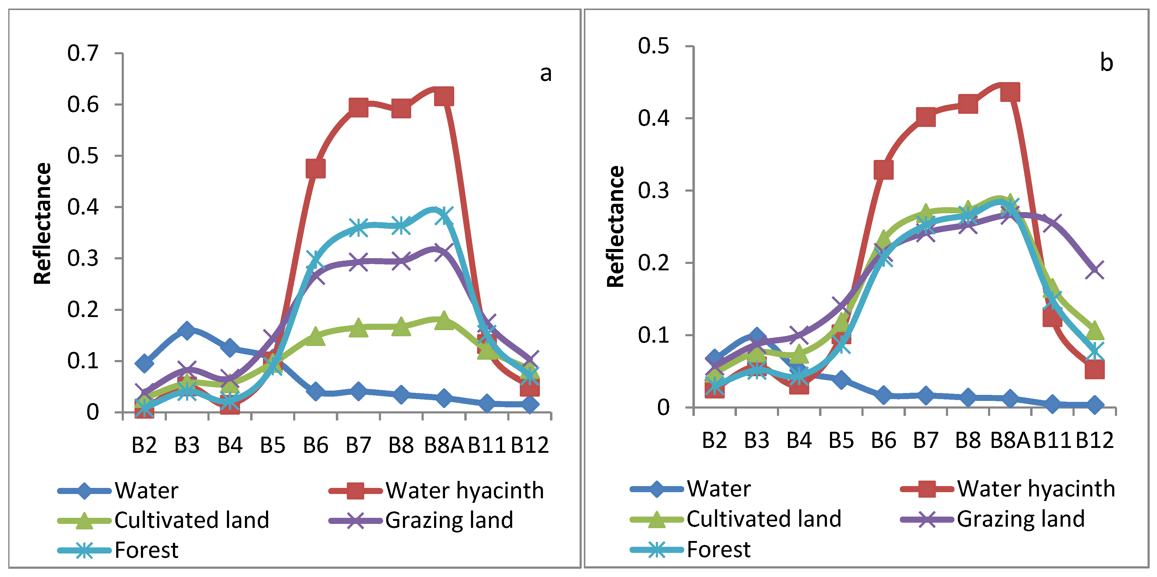
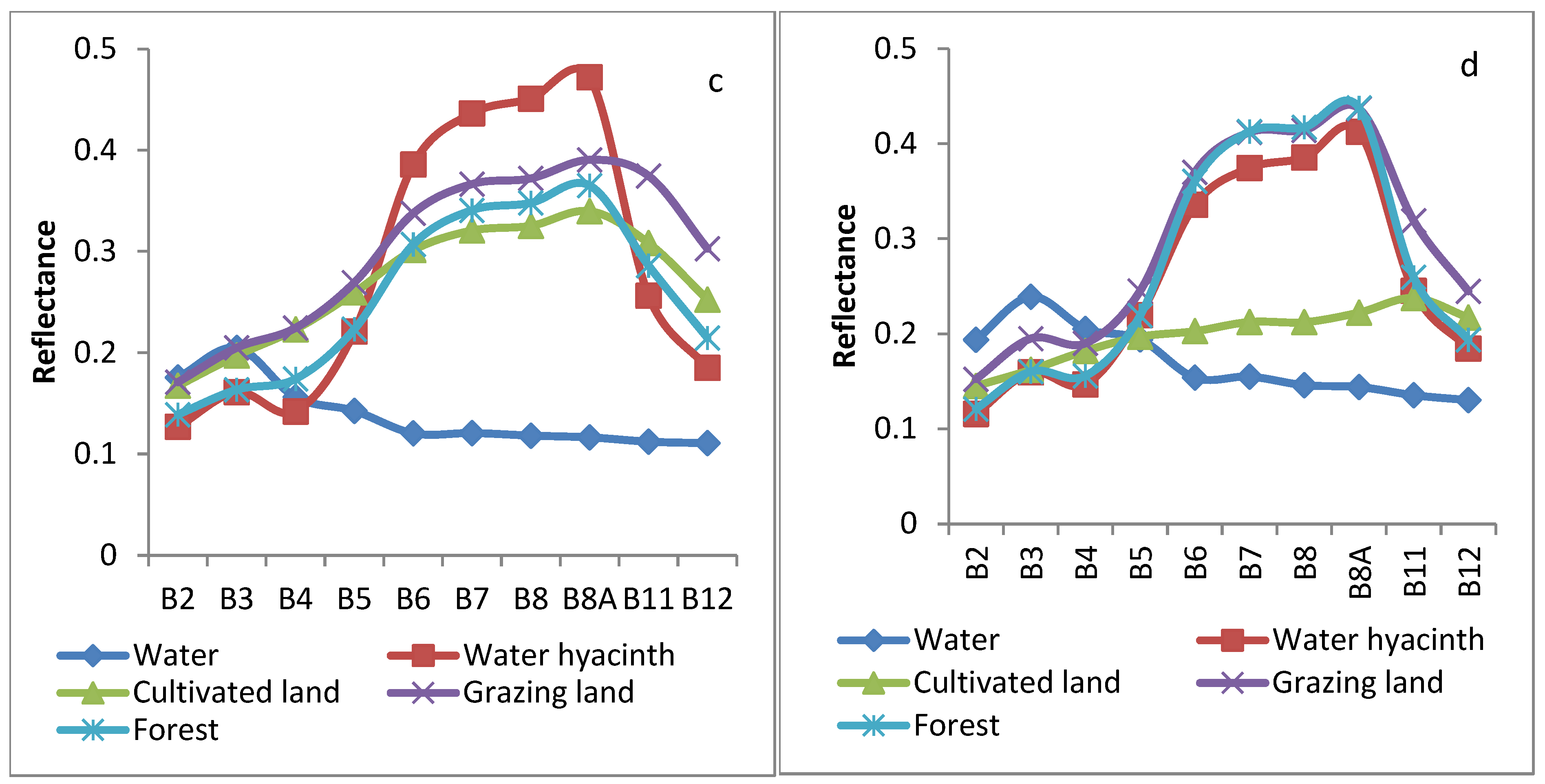
3.1. Water Hyacinth Spectral Reflectance Curve

The seasonal spectral response curves of water, water hyacinth, cultivated land, grazing land, and forest (church forest) in and around Lake Tana from Sentinel 2 were assessed (Figure 2). The spectral reflectance values of each land-use/cover varied with the seasons. Water hyacinth showed the highest reflectance value in the red edge 2 (B6), red edge 3 (B7), near-infrared (B8), and red edge 4 (B8A) bands during autumn, winter, and spring. In the summer season, water hyacinth displayed a relatively lower spectral reflectance value compared with both forest and grazing land in the red edge 2 (B6), red edge 3 (B7), near-infrared (B8), and red edge 4 (B8A) band regions. In the autumn season, the spectral reflectance value of the forest was higher than the cultivated land, grazing land, and water in the red edge 2 (B6), red edge 3 (B7), near-infrared (B8), and red edge 4 (B8A) bands. In winter and spring, the reflectance value of the forest was less than the cultivated land and grazing land, respectively. In general, the spectral reflectance value of water hyacinth was the highest in autumn and the lowest in summer relative to other seasons.

3.2. Performances of the Machine Learning Algorithms: SVM, CART, and RF

All three machine learning classifiers were able to detect the spatial distribution of water hyacinths (E. crassipes) in Lake Tana (Figure 3, Figure 4, Figure 5 and Figure 6). However, when using the SVM and CART on Sentinel 2 images in autumn, spring, and summer, some other vegetation types were misclassified as E. crassipes, as indicated in the black oval shape in the figures (Figure 3b,c, Figure 5b,c and Figure 6b,c, and Table 3). Misclassification of other vegetation was more prevalent in the SVM during the autumn and summer (Table 3, Figure 3c and Figure 6c). Misclassification of other vegetation was also more prevalent in the CART classifiers during spring (Table 3 and Figure 5b). Some water was also misclassified as other vegetation in the CART and RF classifiers during autumn and winter, and this was more prevalent in the CART classifier (Figure 3a,b and Figure 4a,b). Similarly, some E. crassipes were misclassified as other vegetation in the CART and SVM classifiers during winter in the Sentinel 2 data (Figure 4b,c).
During winter, spring, and summer, some other vegetation was classified as E. crassipes in the Landsat 8 CART and SVM classified images, as shown in the black oval shapes in the figures (Figure 4e,f, Figure 5e,f, Figure 6e,f). Misclassification was the highest using the CART for winter and summer (Figure 4e and Figure 6e and Table 3) and using the SVM for spring (Table 3 and Figure 5f). The RF machine learning algorithm detected E. crassipes better than the SVM and CART algorithms in all seasons, as confirmed by field observations (Figure 3a,d, Figure 4a,d, Figure 5a,d, Figure 6a,d). Some water was also misclassified as other vegetation in the CART classifiers across all seasons in the Landsat 8 data (Figure 3e, Figure 4e, Figure 5e, Figure 6e).
The seasonal spatial coverage of E. crassipes and other land-uses/covers in the RF, CART, and SVM methods are shown in Table 3. The area coverage of E. crassipes and other land-uses/covers differed in the three methods in all seasons. In the autumn Sentinel 2 image, there were 2.7 km2 and 6.6 km2 differences in the E. crassipes spatial coverage between the RF and CART methods and between the RF and SVM methods, respectively. This indicated that other land-uses/covers were misclassified as E. crassipes more often using the SVM method compared with other methods during autumn. The largest misclassification of other land-uses/covers occurred in the summer Landsat 8 CART and SVM classified images, with 10.13 km2 and 8.59 km2 area differences from the RF results, respectively (Table 3). In both Sentinel 2 and Landsat 8 data sets, the area coverage of E. crassipes and other land-uses/covers varied between the methods (RF, CART, and SVM) for all seasons. The spatial coverage of E. crassipes varied depending on the algorithm employed and yielded different results using both data sets (Table 3). As a result, evaluating the performance of different algorithms and selecting the most accurate method is critical for accurately estimating the E. crassipes coverage.
The overall accuracy of the Sentinel 2 classified image was greater than 95% using all three methods. The RF had the highest accuracy, ranging from 97 to 99% across all seasons, followed by the CART (97–98%) and SVM (97–98%). Similarly, the kappa coefficients for the RF, SVM, and CART were greater than 0.96 across the seasons, ranging from 0.97 to 0.99 for the RF, 0.96 to 0.98 for the SVM, and 0.96 to 0.97 for the CART. Although the differences in performance between the methods were small, the RF had higher accuracy, while the CART and SVM methods were similar in the Sentinel 2 classified images. The overall accuracies of the Landsat 8 classified images were also greater than 93% in all seasons, ranging from 95 to 98% for the RF, 94 to 96% for the SVM, and 94 to 96% for the CART. The kappa coefficient of the Landsat 8 classified images using all methods was greater than 0.90 for all seasons, ranging from 0.94 to 0.97 for the RF and 0.92 to 0.95 for both the SVM and CART. The differences in accuracy between the methods were also small when using Landsat 8 data, but the RF had the highest accuracy relative to the SVM and CART. Overall accuracy and kappa coefficients for E. crassipes classified image detection were slightly lower when using Landsat 8 data compared with Sentinel 2 data across all three classifiers and all four seasons. In terms of the overall accuracy and kappa coefficient, the RF algorithm slightly outperformed the SVM and CART algorithms across all seasons (Table S1).
Sentinel 2 classified images for E. crassipes detection had a user accuracy of greater than 93% using all three methods (RF, CART, and SVM) for all seasons. The RF had the highest accuracy range of 97–100%, followed by the SVM (96–100%) and CART (94–100%). Similarly, the producer accuracy was greater than 91% for all three methods across all seasons. The average F1 score for the E. crassipes class was 99% for the RF and 98% for both the CART and SVM methods using Sentinel 2 images. Although the user accuracy, producer accuracy, and F1 score differences between the methods were small, the RF had the highest accuracy, while the SVM and CART had almost similar accuracy. The highest F1 score (100–100%) and kappa coefficient (0.97–0.98) from the Sentinel 2 images were found for autumn, while the lowest F1 score (94–95%) and kappa coefficient (0.96–0.97) were found for winter. The user accuracy of Landsat 8 detection ranged from 93 to 98% for the RF, 90 to 99% for the CART, and 88 to 98% for the SVM for all seasons. The producer accuracy using Landsat 8 data for E. crassipes detection also ranged from 96 to 100% for the RF, 94 to 99% for the CART, and 88 to 100% for the SVM. Moreover, the F1 score of Landsat 8 for E. crassipes detection ranged from 95 to 99% for the RF, 92 to 99% for the CART, and 92 to 99% for the SVM (Table S2). The Landsat 8 classified image F1 scores for E. crassipes detection were lower compared with those of the Sentinel 2 images for the RF, SVM, and CART classifiers for all four seasons. In both the Landsat 8 and Sentinel 2 datasets, the RF had the highest F1 score for E. crassipes detection compared with the SVM and CART algorithms, while the SVM and CART had almost the same F1 score for the autumn, winter, spring, and summer classified images. The F1 score of the E. crassipes class was the highest for all three classifiers during autumn. On the other hand, the F1 score and kappa coefficient of E. crassipes detection were the lowest for winter using the Sentinel 2 images and for winter and spring using the Landsat 8 images.

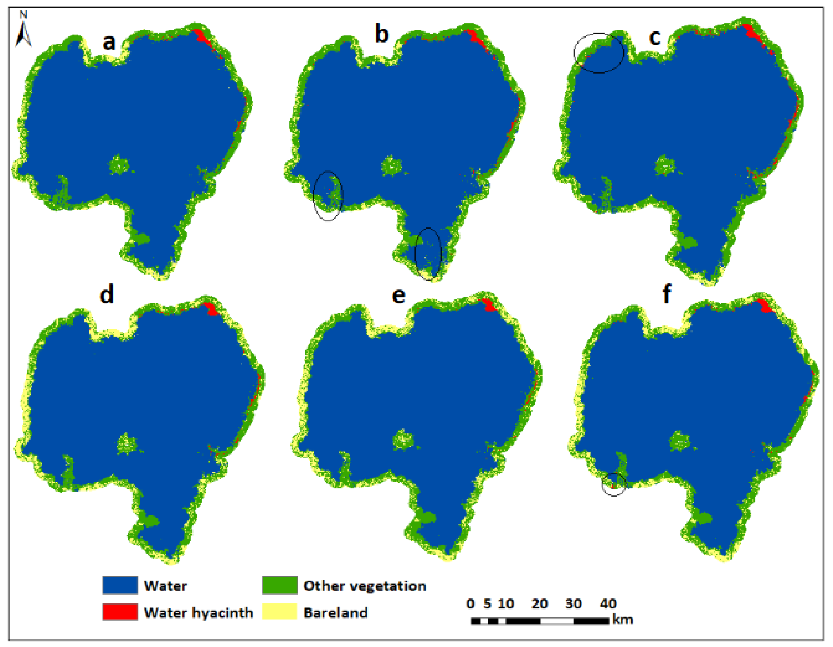
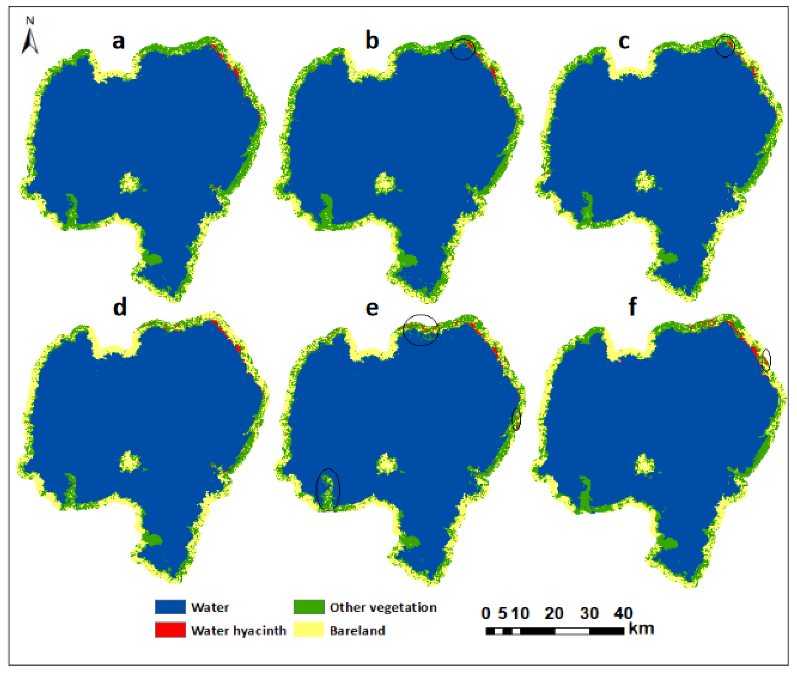
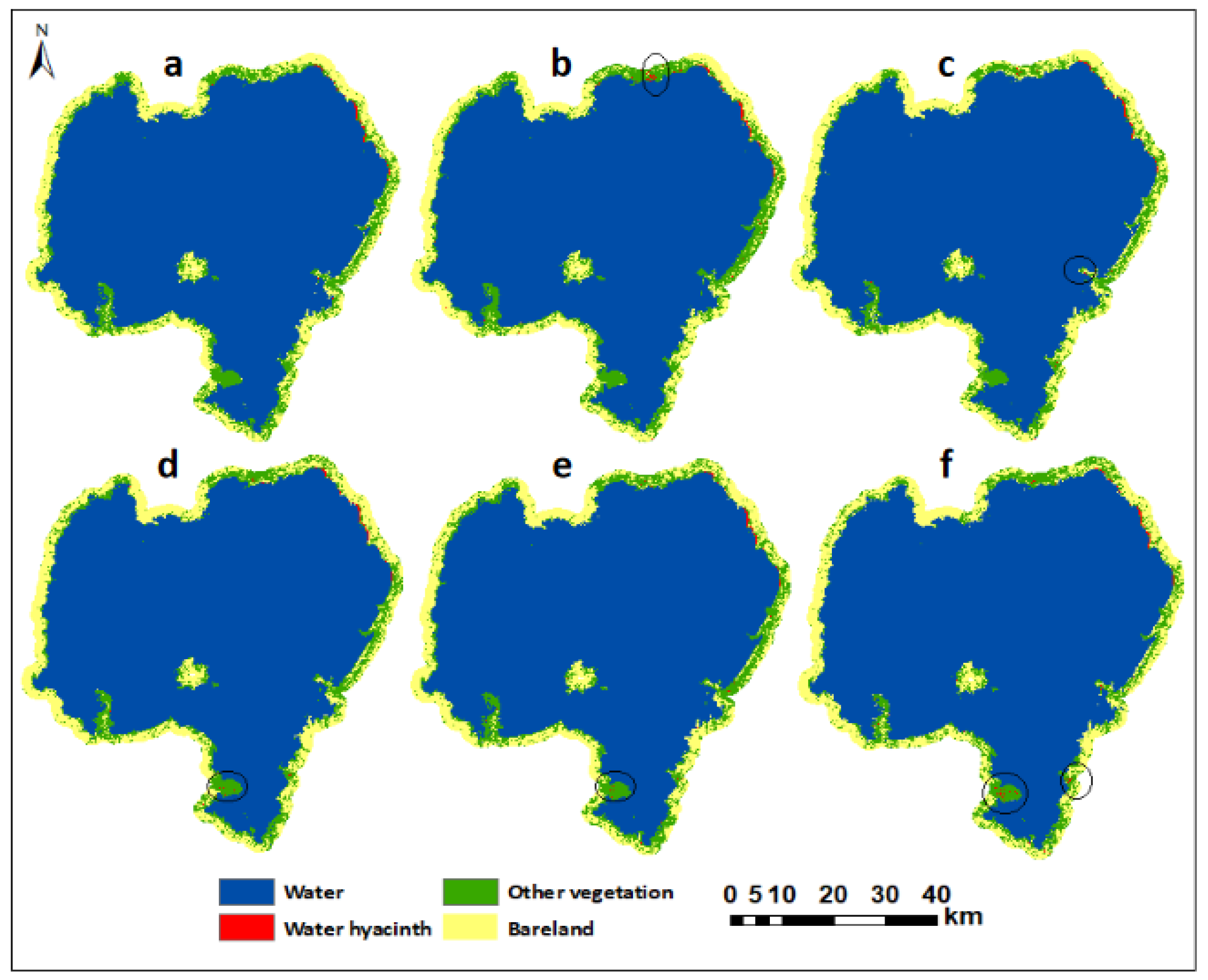
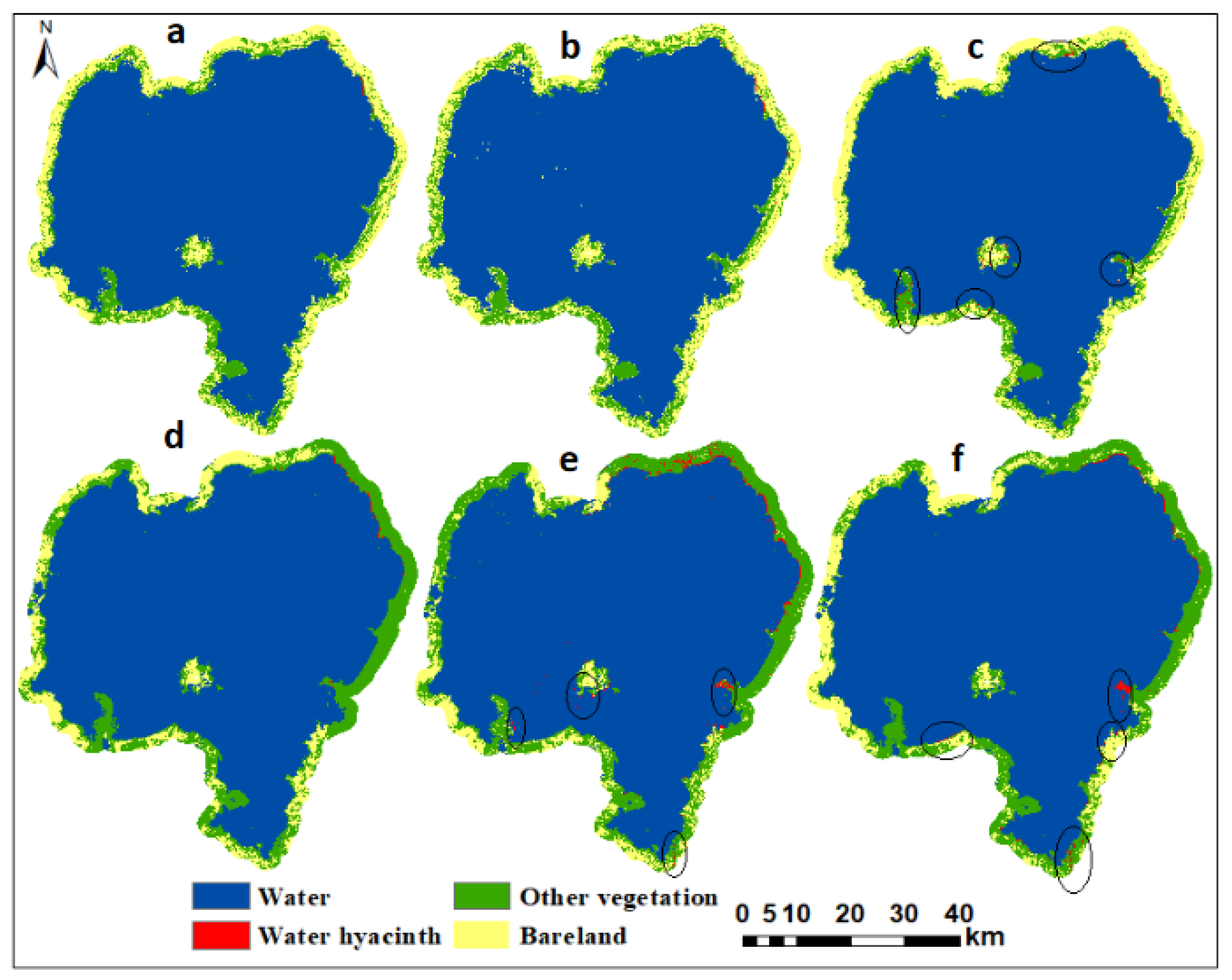
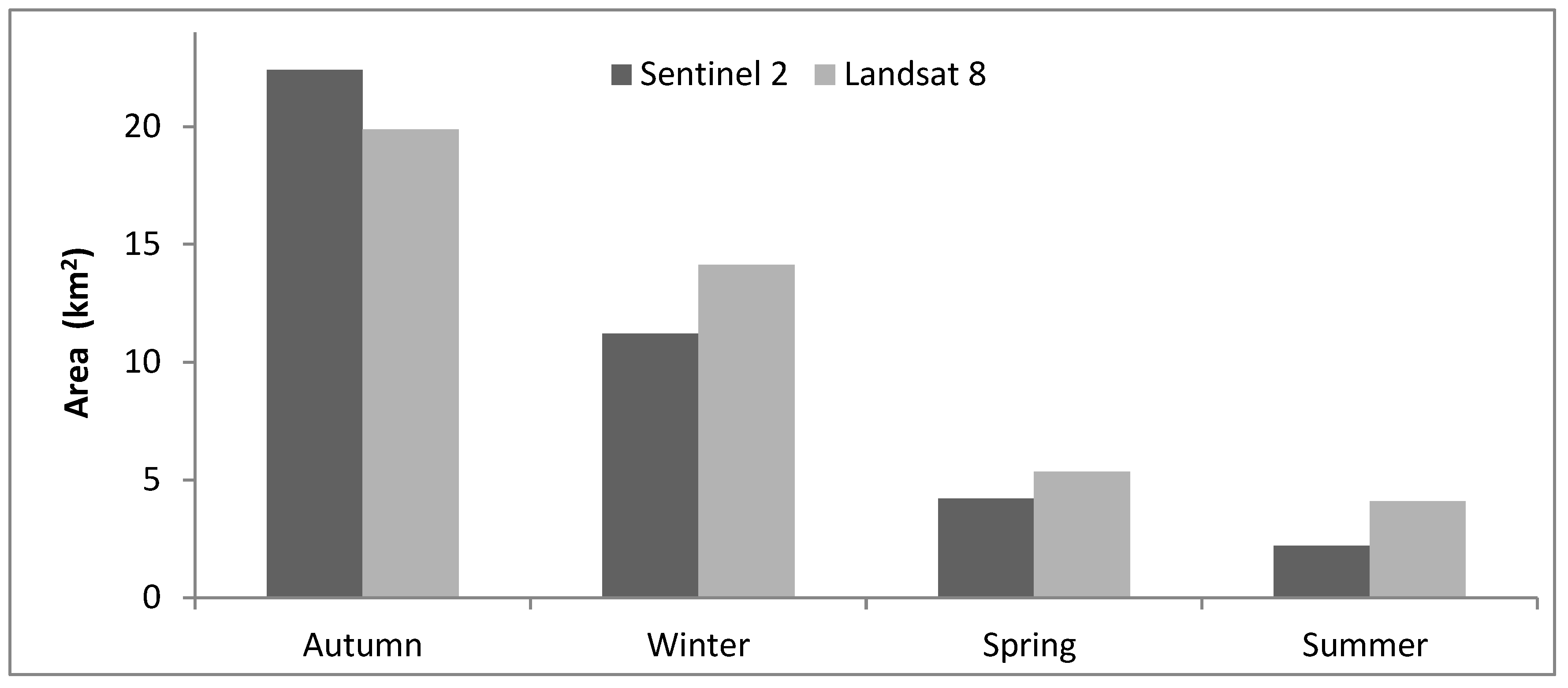
3.3. Water Hyacinth Spatial Coverage

The seasonal spatial coverage of water hyacinth in Lake Tana was estimated from the Sentinel 2 and Landsat 8 images using the random forest (RF) method due to the higher detection performance. The seasonal area coverages of E. crassipes calculated from Sentinel 2 images were 22.4 km2, 11.2 km2, 4.2 km2, and 2.2 km2 for autumn (October 2021), winter (January 2022), spring (March 2022), and summer (June 2022), respectively (Figure 7). The calculated area coverages from Landsat 8 images were 19.87 km2, 14.12 km2, 5.35 km2, and 4.09 km2 for autumn, winter, spring, and summer, respectively. The area coverages of E. crassipes were 12.03 km2 and 4.08 km2 in autumn (2022) and winter (2023), respectively. The spatial coverages of E. crassipes decreased by 50%, 62.5%, and 47.6% from autumn to winter, winter to spring, and spring to summer, respectively, but increased by 81.7% from summer to autumn in the Sentinel 2 images. Similarly, the coverage of E. crassipes decreased by 28.94%, 62.11%, and 23.6% from autumn to winter, winter to spring, and spring to summer, respectively, but increased by 79.4% from summer to autumn in the Landsat 8 images. The E. crassipes spatial coverage was also reduced by 46.3% from 2021 to 2022 in autumn and by 63.6% from 2022 to 2023 in winter. The area coverage of E. crassipes was the highest in autumn (post-rainy season) and the lowest in summer (main rainy season).

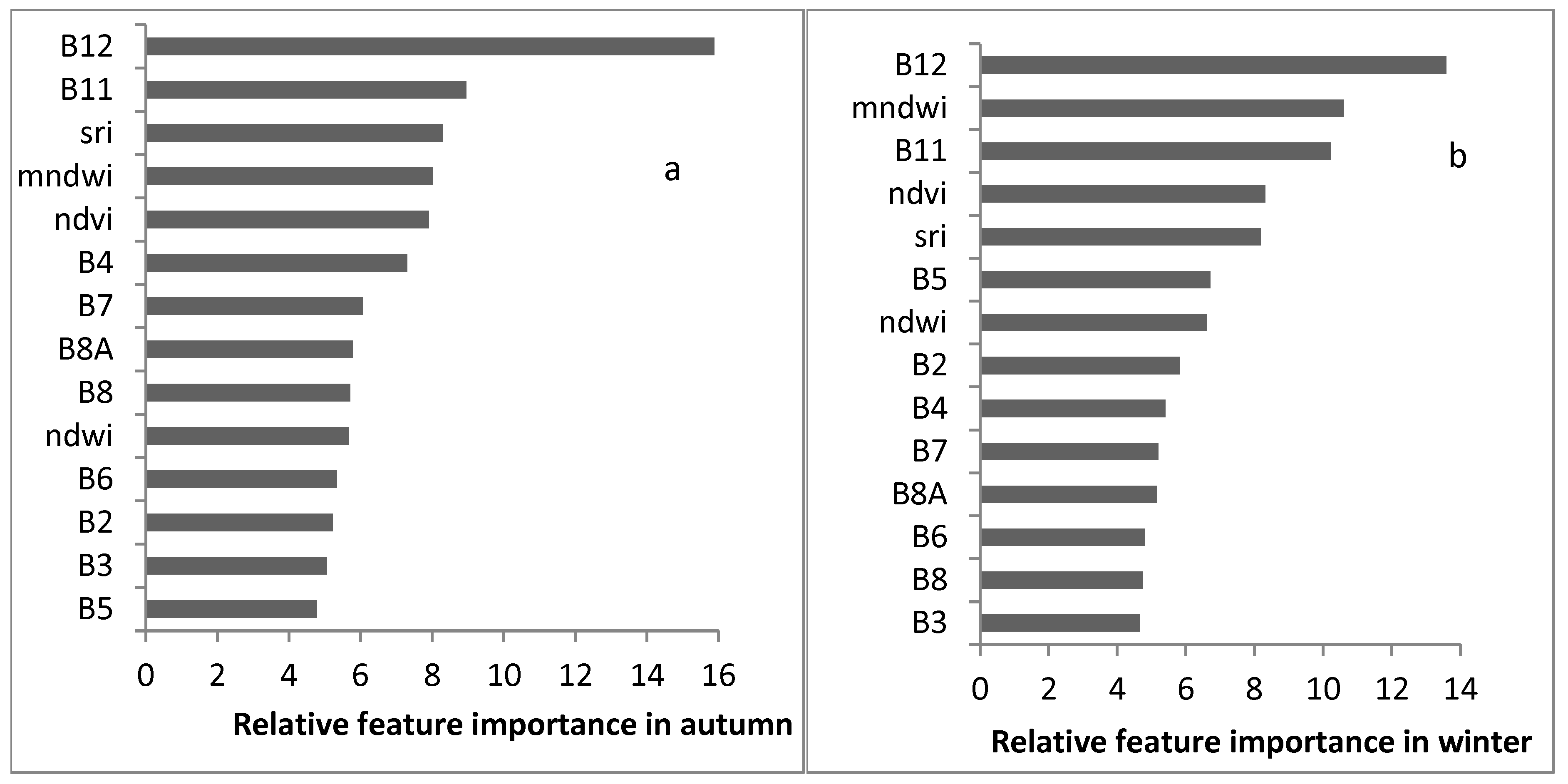
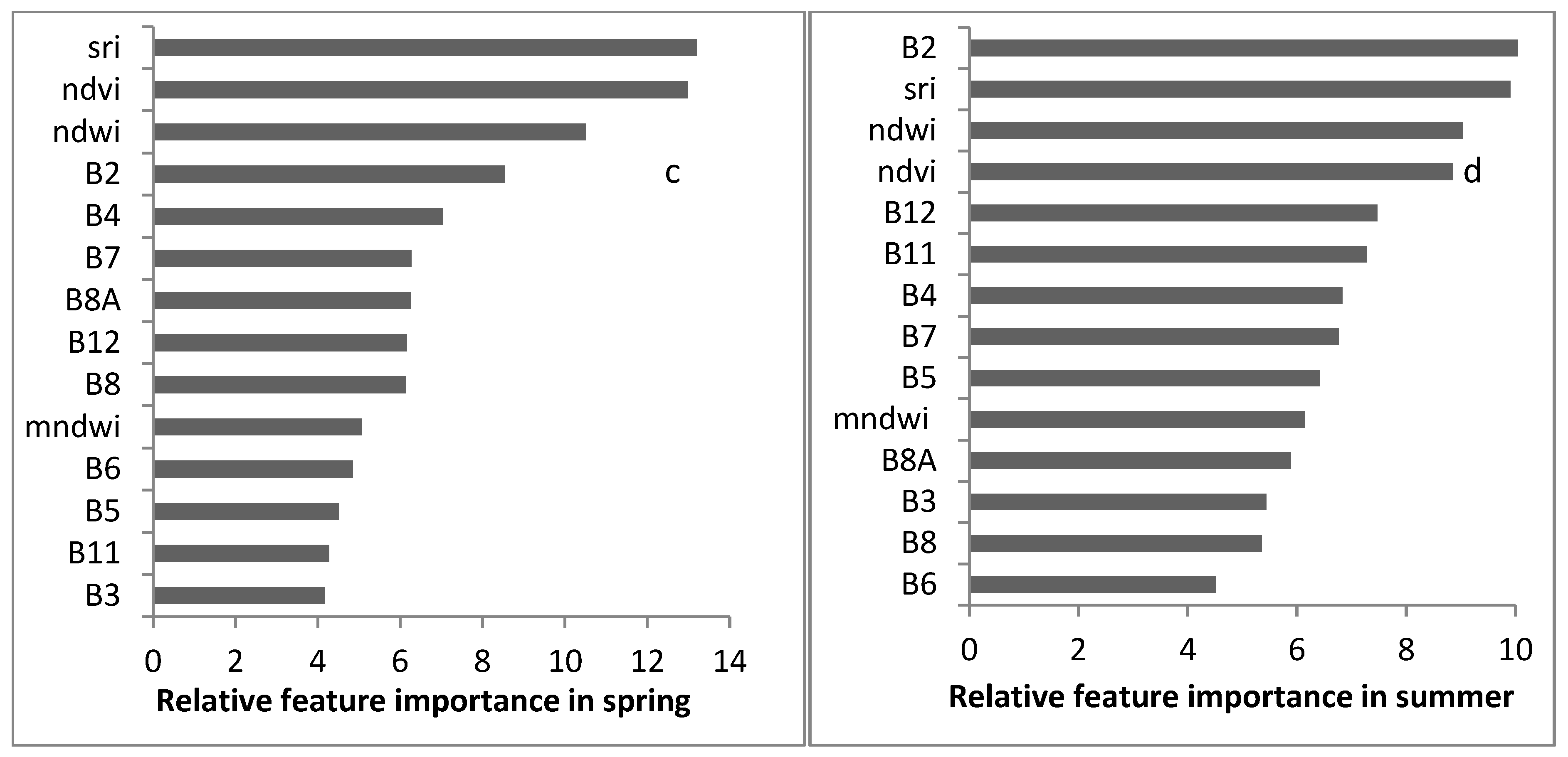
3.4. Feature Importance

The importance of spectral bands and indices in the RF classifier varied with the seasons (Figure 8). In the Sentinel 2 datasets, the spectral indices and spectral bands were found to be the most important variables for classification using the RF classifier. Band 12 (B12) contributed the most to the autumn and spring image classification when compared with other spectral bands and indices. In contrast, the simple ratio index (SRI) and band 2 (B2) contributed the most in spring and summer, respectively.

4. Discussion

Water hyacinth (E. crassipes) is an invasive aquatic plant that can have significant ecological, economic, and social impacts. Detecting and mapping E. crassipes using the most accurate machine learning algorithms on satellite data is critical for decision-makers because it provides accurate and up-to-date information on weed infestations, which will aid in the development of effective aquatic weed management and control strategies. Although machine-learning algorithms were widely used in a variety of interdisciplinary fields, no comparative study was conducted on the performance of machine-learning algorithms for the detection and mapping of E. crassipes in Lake Tana using GEE. The present study compared the performance of three common machine-learning methods for detecting E. crassipes and estimating its seasonal spatial coverage using the most accurate methods in the GEE using medium-resolution multispectral remote sensing images.
Previous studies used satellite images and field measurement reflectance to distinguish E. crassipes from other land-use/cover types. For instance, Datta et al. [5] used Sentinel 2 images to distinguish E. crassipes from other aquatic macrophytes, where submerged macrophytes were distinguished by their lower reflectance in the near-infrared band. Verma et al. [68] also measured field reflectance in several southern Texas waterways and revealed that E. crassipes had higher near-infrared reflectance than related plant species and water. Similarly, in the present study, E. crassipes had higher reflectance values in the near-infrared and red edge regions of autumn, winter, and spring Sentinel 2 images (Figure 2). In summer, E. crassipes showed a lower spectral reflectance value than forest and grazing land in these band regions.
Each machine-learning algorithm has its own set of advantages and disadvantages [36]. An SVM is hyperparameter sensitive, whereas an RF is more robust and less affected by parameters and noise [69,70]. On the other hand, the performance of an SVM is good when few training sample points are available [71]. A CART is also sensitive to the sample size [36]. In both the Landsat 8 and Sentinel 2 datasets, the RF outperformed the SVM and CART, whereas the CART and SVM algorithm performances were similar in terms of the F1 score, overall accuracy, and kappa coefficient for detection and mapping for all seasons. This difference is attributable to the fact that the RF classifier is less sensitive to noise and parameters. Similarly, Mukarugwiro et al. [72] revealed that an RF outperforms an SVM in terms of overall accuracy for E. crassipes detection in Rwandan water. Likewise, some previous studies reported that an RF outperforms both SVM and CART classifiers in terms of overall accuracy for land-use/cover mapping [36,73]. Shetty et al. [73] also revealed that CART and SVM classifiers performed similarly for land-use/cover classification. Further, Shao and Lunetta [71] claimed that an SVM outperforms CART classifiers for land-use/cover classification using MODIS images with limited training data points. The discrepancy between the results was likely because an SVM performs well with small training samples. The accuracy of the classification does not necessarily increase with increasing spatial and spectral resolution [74]. In the present study, the accuracy of E. crassipes detection increased as the spectral and spatial resolution of the satellite dataset increased. Sentinel 2 images produced a higher F1 score, overall accuracy, and kappa coefficients compared with Landsat 8 images. The results of this study were similar to Thamaga and Dube [75], who reported that Sentinel 2 outperformed Landsat 8 in mapping E. crassipes in South Africa’s Greater Letaba river system due to the higher spatial and spectral resolution.
The RF, CART, and SVM machine learning algorithms were all able to detect and distinguish E. crassipes invasive aquatic weed in Lake Tana (Figure 3, Figure 4, Figure 5 and Figure 6). However, when using the SVM and CART on the autumn, spring, and summer Sentinel 2 images, some other vegetation types were misclassified as E. crassipes because dense vegetation had a nearly similar spectral reflectance to E. crassipes. Some water was also misclassified as other vegetation when using the CART and RF classifiers on the autumn and winter Sentinel 2 images, which could be attributed to high concentrations of algae or phytoplankton in the lake water. The average overall accuracy of the RF, CART, and SVM in the present study was greater than 95% for the Sentinel 2 images and greater than 90% for the Landsat 8 images. Although the difference in accuracy between the three methods was small, there was a significant difference in the final estimation of spatial coverage for E. crassipes and other land-uses/covers (Table 3). The average overall accuracy of the classifiers when using the Sentinel 2 images was 97.8%, while the average overall accuracy of the classifiers when using the Landsat 8 images was 95.5%. Though the difference in accuracy between the two was not significant, there was a meaningful difference in the estimation of land-use/cover and water hyacinth area coverage (Table 3). During autumn, the F1 score of the E. crassipes class was highest across all classifiers; however, the E. crassipes class had the lowest F1 score and kappa coefficient during winter when using Sentinel 2 images and during winter and spring when using Landsat 8 images. The low F1 score and kappa coefficient of the E. crassipes class during winter were attributable to the presence of different irrigated crops around Lake Tana. Some dense irrigated crops have similar reflectance values to the invasive weed, which made it difficult to distinguish the E. crassipes from the crops. Additionally, the leaves of E. crassipes change color and become dry during the winter and spring, which contributes to the classification accuracy due to the change in reflectance. On the other hand, when the E. crassipes leaves change to bright green (high reflectance) at the end of the main rainy season (autumn) [41], the detection accuracy is substantially increased.
The spatial coverage of E. crassipes was at a maximum and minimum during the post-rainy season and rainy season, respectively. The increased area coverage of E. crassipes during the post-rainy season was consistent with the findings of Worqlul et al. [1] and Cai et al. [76], who reported a significant increase in area coverage during autumn and a decrease during summer. In contrast, Damtie et al. [38] reported that the E. crassipes area coverage was the highest in winter and the lowest in spring in 2019. The discrepancy may be attributed to the management and E. crassipes removal practices employed by the government and the local community. In the present study, the area coverage of E. crassipes decreased significantly from winter to spring, with a decrease of 62.5% using the Sentinel 2 images. Conversely, a significant increase in area coverage was observed from summer to autumn, with an increase of 81.7%. Similarly, the Landsat 8 images showed a large decrease in the E. crassipes area coverage (62.11%) from winter to spring, while there was a large increase (79.4%) from summer to autumn. The population of E. crassipes grew rapidly from summer to autumn and decreased from autumn to summer, indicating that summer was the season of the most rapid growth for the weed population. The reduction in area coverage from autumn to summer may have been due to the removal of E. crassipes by various stakeholders, in addition to life cycle effects and increased dryness. The ability to monitor these changes could support within-year management decisions.
During the post-rainy season, the highest population of E. crassipes was observed around the northeastern shore of Lake Tana, where the distribution increased to the lake’s eastern shore during the dry and minor rainy seasons (Figure 3, Figure 4, Figure 5 and Figure 6). During the post-rainy season, winds and subsequent waves can transport the weed to the northeastern sector of the lake [76]. While this study only investigated seasonal changes in the total area coverage, accurate monitoring of E. crassipes using remote sensing will allow for the assessment of spatiotemporal changes in coverage between different regions of the Lake Tana shoreline, both within seasons and across years. Detecting E. crassipes infestation from remote sensing data using machine learning methods during different seasons can provide a more comprehensive understanding of the seasonal variability of the infestation and will contribute to the larger effort of improving environmental assessment and monitoring through remote sensing data, as it provides a more accurate, cost-effective, and efficient method of monitoring water hyacinth infestations in large water bodies, such as Lake Tana.

5. Machine Learning Algorithms Related Work in Water Hyacinth Detection

In recent years, some studies employed machine learning methods for the detection of water hyacinth (E. crassipes) (Table 4). A study by Dube et al. [77] used a discriminant analysis (DA) and partial least-squares discriminant analysis (PLS-DA) machine learning classification ensemble for E. crassipes detection, which was applied to Landsat 8 data. The DA and PLS-DA machine learning classification ensemble was able to detect E. crassipes with an accuracy of 95%. Similarly, a study by Pádua et al. [78] used random forest (RF), support vector machine (SVM), Gaussian naive Bayes (NB), k-nearest neighbors (KNN), and artificial neural network (ANN) algorithms on unmanned aerial vehicle (UAV) and Sentinel 2 data. From these different classifiers, the study reported that the RF performed the best, with an overall accuracy of 94%, while the SVM performed the worst, with an overall accuracy of 87%. The study by Mukarugwiro et al. [72] used an RF and SVM for E. crassipes detection and trained the methods using Landsat 8 images. The study also reported that the RF (85%) outperformed the SVM (65%) for E. crassipes detection in Rwandan water bodies. Thamaga and Dube [79] used linear discriminant analysis (LDA) applied to Sentinel 2 data to map the seasonal dynamics of invasive E. crassipes in the Greater Letaba river system in Limpopo Province, South Africa. The LDA was able to map E. crassipes with an overall accuracy of 80.79% during the wet season and 79.04% during the dry season. Thamaga and Dube [75] also used discriminant analysis (DA) to test the capability of the Landsat 8 Operational Land Imager (OLI) and Sentinel-2 MultiSpectral Instrument (MSI) for E. crassipes detection in a river system. They revealed that E. crassipes in small reservoirs can be mapped with an overall accuracy of 68.44% and 77.56% using Landsat 8 and Sentinel-2 data, respectively. In 2022, Ade et al. [80] employed an RF to map E. crassipes using Sentinel-2 data and obtained an overall accuracy of 90%, with class-specific accuracies ranging from 79–91%. Moreover, Singh et al. [81] used a hierarchical classification approach on medium-resolution multispectral satellite data for mapping E. crassipes, resulting in an overall accuracy of 93% and an F1 score of 87%. In conclusion, a variety of machine learning methods were used in recent years to detect E. crassipes with varying degrees of accuracy using various data sources. Overall, these previous studies showed that machine learning methods have the potential to aid in the detection of E. crassipes. In the present study, all methods (RF, CART, and SVM) achieved greater than 90% overall accuracy on both Landsat 8 and Sentinel 2 images, indicating that all methods have the potential to aid in the detection of Eichhornia Crassipes when compared with previously used methods. However, the random forest method had the highest accuracy.

6. Conclusions

The performances of RF, SVM, and CART machine learning algorithms for water hyacinth (E. crassipes) detection in different seasons were compared using Landsat 8 and Sentinel 2 images on the GEE in Lake Tana, Ethiopia. The RF, SVM, and CART machine learning algorithms were able to detect E. crassipes in Landsat 8 and Sentinel 2 images for all seasons. Using Sentinel 2 images, all methods achieved greater than 95% overall accuracy and greater than 93% F1 score across all seasons. Similarly, using Landsat 8 images, all methods achieved greater than 90% overall accuracy and an 89% F1 score. Although the difference in performance between the methods was small, the RF method was the most accurate, while the SVM and CART methods had the same accuracy across all seasons. The RF outperformed the SVM and CART algorithms in terms of overall accuracy, kappa coefficient, and F1 score across all four seasons, whereas the CART and SVM had similar performances when using both the Landsat 8 and Sentinel 2 images. The average overall accuracy of the classifiers for the Sentinel 2 images was 97.8%, while the average overall accuracy of the classifiers for the Landsat 8 images was 95.5%. The E. crassipes detection accuracy was slightly higher when using the Sentinel 2 images than the Landsat 8 images. The presence of red edge bands in the Sentinel 2 images enabled better detection of E. crassipes than in the Landsat 8 images. Although the difference in accuracy between the methods and between sensors was small, there was a significant difference in the final estimation of the area coverage for E. crassipes between the three methods. The spatial coverage of E. crassipes was reduced by 46.3% from 2021 to 2022 in autumn and by 63.6% from 2022 to 2023 in winter. There was a large decrease in the E. crassipes area coverage (62.5%) from winter to spring, whereas there was a large increase (81.7%) from summer to autumn. E. crassipes had a high spatial coverage in the post-rainy season and a low spatial coverage in the main rainy season. The results of this study suggested that of the three classifiers evaluated, the RF was found to be best for E. crassipes detection, and because of the highest F1 score and kappa coefficient, autumn was the best season for E. crassipes detection and mapping in Lake Tana. Identifying suitable machine learning methods by comparing their performances and estimating the seasonal spatial coverage using the most accurate method will improve decision-making by providing accurate and up-to-date information on E. crassipes infestations, which will aid in the development of effective management and control strategies. In the present study, only medium-resolution multispectral remote sensing images (Landsat 8 and Sentinel 2) were used to compare machine-learning algorithms for E. crassipes detection and seasonal spatial coverage estimation. These methods cannot identify small and fragmented E. crassipes weeds using medium-resolution satellite data. In the future, high-resolution (less than 10 m) satellite data, such as Maxar satellite imagery and SkySat satellite imagery, should be investigated for E. crassipes detection using machine learning algorithms.

Supplementary Materials

The following supporting information can be downloaded at: https://www.mdpi.com/article/10.3390/w15050880/s1, Figure S1: Machine learning classifier comparison in autumn (October 2022): Sentinel 2 (a) RF, (b) CART, (c) SVM. Black oval shape in the figure represents the area of misclassification; Figure S2: Machine learning classifier comparison in winter (January 2023): Sentinel 2 (a) RF, (b) CART, (c) SVM. Black oval shape in the figure represents the area of misclassification; Table S1: Overall accuracy and kappa coefficient of RF, CART, and SVM classifiers in autumn, winter, spring, and summer Sentinel 2 and Landsat 8 images; Table S2: F1 score, user and producer accuracy of water hyacinth class in autumn, winter, spring, and summer seasons using RF, CART, and SVM algorithms in Sentinel 2 and Landsat 8 datasets; Table S3. Performance of RF, CART and SVM methods.

Author Contributions

Conceptualization, G.B., J.C. and V.S.K.; methodology, G.B. and M.M; software, G.B.; validation, G.B., M.M. and V.S.K.; formal analysis, J.C.; investigation, G.B.; resources, S.A.L. and V.S.K.; data curation, G.B.; writing—original draft preparation, G.B.; writing—review and editing, J.C., M.M., S.A.L. and V.S.K.; visualization, G.B.; supervision, V.S.K. and, H.I.; project administration, K.I.; funding acquisition, H.I. and K.I. All authors have read and agreed to the published version of the manuscript.

Funding

This research was supported by Science and Technology Research Partnership for Sustainable Development (SATREPS; Grant Number JPMJSA2005) funded by Japan Science and Technology Agency (JST)/Japan International Cooperation Agency (JICA).

Institutional Review Board Statement

Not applicable.

Informed Consent Statement

Not applicable.

Data Availability Statement

The datasets are available upon reasonable request from the corresponding author.

Conflicts of Interest

The authors declare no conflict of interest.

References

  1. Worqlul, A.W.; Ayana, E.K.; Dile, Y.T.; Moges, M.A.; Gitaw, M.G.; Tegegne, G.; Kibret, S. Spatiotemporal Dynamics and Environmental Controlling Factors of the Lake Tana Water Hyacinth in Ethiopia. Remote Sens. 2020, 12, 2706. [Google Scholar] [CrossRef]
  2. Goshu, G.; Tewabe, D.; Adugna, B.T. Spatial and temporal distribution of commercially important fish species of Lake Tana, Ethiopia. Ecohydrol. Hydrobiol. 2010, 10, 231–240. [Google Scholar] [CrossRef]
  3. Karim, D.; Rachid, L.; Mamourou, D.; Ssam, M.J.H. Production and oil-emulsion formulation of Cadophora malorum and Alternaria jacinthicola, two biocontrol agents against Water Hyacinth (Eichhornia crassipes). Afr. J. Microbiol. Res. 2011, 5, 924–929. [Google Scholar] [CrossRef] [Green Version]
  4. Piyaboon, O.; Pawongrat, R.; Unartngam, J.; Chinawong, S.; Unartngam, A. Pathogenicity, host range and activities of a secondary metabolite and enzyme from Myrothecium roridum on water hyacinth from Thailand. Weed Biol. Manag. 2016, 16, 132–144. [Google Scholar] [CrossRef]
  5. Datta, A.; Maharaj, S.; Prabhu, G.N.; Bhowmik, D.; Marino, A.; Akbari, V.; Rupavatharam, S.; Sujeetha, J.A.R.P.; Anantrao, G.G.; Poduvattil, V.K.; et al. Monitoring the Spread of Water Hyacinth (Pontederia crassipes): Challenges and Future Developments. Front. Ecol. Evol. 2021, 9, 1–8. [Google Scholar] [CrossRef]
  6. Rakotoarisoa, T.F. Use of Water Hyacinth (Eichhornia crassipes) in Poor and Remote Regions-A Case Study From Lake Alaotra. Ph.D. Thesis, University of Hildesheim, Hildesheim, Gremany, 2017. [Google Scholar]
  7. Hill, M.P. The impact and control of alien aquatic vegetation in South African aquatic ecosystems. Afr. J. Aquat. Sci. 2003, 28, 19–24. [Google Scholar] [CrossRef]
  8. UNEP. Water hyacinth—Can its aggressive invasion be controlled? Environ. Dev. 2013, 7, 139–154. [Google Scholar] [CrossRef]
  9. Seburanga, J.L.; Kaplin, B.A.; Bizuru, E.; Mwavu, E.N.; Gatesire, T. Control of water hyacinth (Eichhornia crassipes) in Rwanda: A survey of local residents’ perceptions. In Proceedings of the 19th Australasian Weeds Conference, Hobart, Australia, 1–4 September 2014; Available online: https://nru.uncst.go.ug/handle/123456789/5735 (accessed on 20 October 2022).
  10. Meerhoff, M.; Fosalba, C.; Bruzzone, C.; Mazzeo, N.; Noordoven, W.; Jeppesen, E. An experimental study of habitat choice by Daphnia: Plants signal danger more than refuge in subtropical lakes. Freshw. Biol. 2006, 51, 1320–1330. [Google Scholar] [CrossRef]
  11. Mironga, J.M.; Mathooko, J.M.; Onywere, S.M. Effects of spreading patterns of water hyacinth (Eichhornia crassipes) on zooplankton population in Lake Naivasha, Kenya. Int. J. Dev. Sustain. 2014, 3, 1971–1987. [Google Scholar]
  12. Villamagna, A.M.; Murphy, B.R. Ecological and socio-economic impacts of invasive water hyacinth (Eichhornia crassipes): A review. Freshw. Biol. 2010, 55, 282–298. [Google Scholar] [CrossRef]
  13. Getnet, H.; Kifle, D.; Fetahi, T. Impact of water hyacinth (Eichhornia crassipes) on water quality and phytoplankton community structure in the littoral region of Koka Reservoir, Ethiopia. Int. J. Fish Aquat. Stud. 2021, 9, 266–276. [Google Scholar]
  14. Damtie, Y.A.; Mengistu, D.A.; Meshesha, D.T. Spatial coverage of water hyacinth (Eichhornia crassipes (Mart.) Solms) on Lake Tana and associated water loss. Heliyon 2021, 7, e08196. [Google Scholar] [CrossRef] [PubMed]
  15. Dejen, E.; Sibbing, F.A.; Vijverberg, J. Reproductive strategies of two sympatric “small barbs” (Barbus humilis and B. tanapelagius, Cyprinidae) in Lake Tana, Ethiopia. Neth. J. Zool. 2003, 52, 281–299. [Google Scholar] [CrossRef]
  16. Setegn, S.G.; Srinivasan, R.; Dargahi, B. Hydrological Modelling in the Lake Tana Basin, Ethiopia Using SWAT Model. Open Hydrol. J. 2008, 2, 49–62. [Google Scholar] [CrossRef] [Green Version]
  17. Wondie, A.; Mengistu, S.; Vijverberg, J.; Dejen, E. Seasonal variation in primary production of a large high altitude tropical lake (Lake Tana, Ethiopia): Effects of nutrient availability and water transparency. Aquat. Ecol. 2007, 41, 195–207. [Google Scholar] [CrossRef]
  18. Anteneh, W.; Mengist, M.; Wondie, A.; Tewabe, D.; WoldeKidan, W.; Assefa, A.; Engida, W. Water Hyacinth Coverage Survey Report on Lake Tana; Technical Report Series 1; Bahir Dar University: Bahir Dar, Ethiopia, 2015. [Google Scholar]
  19. Asmare, T.; Demissie, B.; Nigusse, A.G.; GebreKidan, A. Detecting Spatiotemporal Expansion of Water Hyacinth (Eichhornia crassipes) in Lake Tana, Northern Ethiopia. J. Indian Soc. Remote Sens. 2020, 48, 751–764. [Google Scholar] [CrossRef]
  20. Poppe, L.; Frankl, A.; Poesen, J.; Admasu, T.; Dessie, M.; Adgo, E.; Deckers, J.; Nyssen, J. Geomorphology of the Lake Tana basin, Ethiopia. J. Maps 2013, 9, 431–437. [Google Scholar] [CrossRef] [Green Version]
  21. Tibebe, D.; Kassa, Y.; Melaku, A.; Lakew, S. Investigation of spatio-temporal variations of selected water quality parameters and trophic status of Lake Tana for sustainable management, Ethiopia. Microchem. J. 2019, 148, 374–384. [Google Scholar] [CrossRef]
  22. Damtie, Y.A.; Berlie, A.B.; Gessese, G.M.; Ayalew, T.K. Characterization of water hyacinth (Eichhornia crassipes (Mart.) Solms) biomass in Lake Tana, Ethiopia. All Life 2022, 15, 1126–1140. [Google Scholar] [CrossRef]
  23. Asmare, E. Current Trend of Water Hyacinth Expansion and Its Consequence on the Fisheries around North Eastern Part of Lake Tana, Ethiopia. J. Biodivers. Endanger. Species 2017, 5, 2–5. [Google Scholar] [CrossRef]
  24. Ritchie, J.C.; Zimba, P.V.; Everitt, J.H. Remote Sensing Techniques to Assess Water Quality. Photogramm. Eng. Remote Sens. 2003, 69, 695–704. [Google Scholar] [CrossRef] [Green Version]
  25. Hoshino, B.; Karamalla, A.; Manayeva, K.; Yoda, K.; Suliman, M.; Elgamri, M.; Nawata, H.; Yasuda, H. Evaluating the invasion strategic of Mesquite (Prosopis juliflora) in eastern Sudan using remotely sensed technique. J. Arid. Land Stud. 2012, 22, 1–4. [Google Scholar]
  26. Mucheye, T.; Haro, S.; Papaspyrou, S.; Caballero, I. Water quality and water hyacinth monitoring with the Sentinel- 2A / B satellites in Lake Tana (Ethiopia). Remote Sens. 2022, 14, 4921. [Google Scholar] [CrossRef]
  27. Sun, Z.; Xu, R.; Du, W.; Wang, L.; Lu, D. High-resolution urban land mapping in China from sentinel 1A/2 imagery based on Google Earth Engine. Remote Sens. 2019, 11, 752. [Google Scholar] [CrossRef] [Green Version]
  28. Gibson, R.; Danaher, T.; Hehir, W.; Collins, L. A remote sensing approach to mapping fire severity in south-eastern Australia using sentinel 2 and random forest. Remote Sens. Environ. 2020, 240, 111702. [Google Scholar] [CrossRef]
  29. Pan, X.; Zhang, C.; Xu, J.; Zhao, J. Simplified object-based deep neural network for very high resolution remote sensing image classification. ISPRS J. Photogramm. Remote Sens. 2021, 181, 218–237. [Google Scholar] [CrossRef]
  30. Sheykhmousa, M.; Mahdianpari, M.; Ghanbari, H.; Mohammadimanesh, F.; Ghamisi, P.; Homayouni, S. Support Vector Machine Versus Random Forest for Remote Sensing Image Classification: A Meta-Analysis and Systematic Review. IEEE J. Sel. Top. Appl. Earth Obs. Remote Sens. 2020, 13, 6308–6325. [Google Scholar] [CrossRef]
  31. Liu, L.; Guo, Y.; Li, Y.; Zhang, Q.; Li, Z.; Chen, E.; Yang, L.; Mu, X. Comparison of Machine Learning Methods Applied on Multi-Source Medium-Resolution Satellite Images for Chinese Pine (Pinus tabulaeformis) Extraction on Google Earth Engine. Forests 2022, 13, 677. [Google Scholar] [CrossRef]
  32. Rodriguez-Galiano, V.F.; Ghimire, B.; Rogan, J.; Chica-Olmo, M.; Rigol-Sanchez, J.P. An assessment of the effectiveness of a random forest classifier for land-cover classification. ISPRS J. Photogramm. Remote Sens. 2012, 67, 93–104. [Google Scholar] [CrossRef]
  33. Ahmad, M.W.; Reynolds, J.; Rezgui, Y. Predictive modelling for solar thermal energy systems: A comparison of support vector regression, random forest, extra trees and regression trees. J. Clean Prod. 2018, 203, 810–821. [Google Scholar] [CrossRef]
  34. Zhao, Q.; Yu, S.; Zhao, F.; Tian, L.; Zhao, Z. Comparison of machine learning algorithms for forest parameter estimations and application for forest quality assessments. For. Ecol. Manag. 2019, 434, 224–234. [Google Scholar] [CrossRef]
  35. Pham, T.D.; Yokoya, N.; Xia, J.; Ha, N.T.; Le, N.N.; Nguyen, T.T.T.; Dao, T.H.; Vu, T.T.P.; Takeuchi, W. Comparison of Machine Learning Methods for Estimating Mangrove Above-Ground Biomass Using Multiple Source Remote Sensing Data in the Red River Delta Biosphere Reserve, Vietnam. Remote Sens. 2020, 12, 1334. [Google Scholar] [CrossRef] [Green Version]
  36. Loukika, K.N.; Keesara, V.R.; Sridhar, V. Analysis of Land Use and Land Cover Using Machine Learning Algorithms on Google Earth Engine for Munneru River Basin, India. Sustainability 2021, 13, 13758. [Google Scholar] [CrossRef]
  37. Belgiu, M.; Dragu, L. Random forest in remote sensing: A review of applications and future directions gut. ISPRS J. Photogramm. Remote Sens. 2016, 114, 24–31. [Google Scholar] [CrossRef]
  38. Cortes, C.; Vapnik, V. Support-vector networks. Mach. Learn. 1995, 20, 273–297. [Google Scholar] [CrossRef]
  39. Brieman, L.; Friedman, J.H.; Olshen, R.A.; Stone, C.J. Classification and Regression Trees, 1st ed.; Routledge: London, UK, 1984; Volume 45, pp. 5–32. [Google Scholar]
  40. Sewak, M.; Sahay, S.K.; Rathore, H. Comparison of deep learning and the classical machine learning algorithm for the malware detection. In Proceedings of the 19th IEEE/ACIS International Conference on Software Engineering, Artificial Intelligence, Networking and Parallel/Distributed Computing (SNPD), Busan, Korea, 27–29 June 2018; pp. 293–296. [Google Scholar] [CrossRef] [Green Version]
  41. Dersseh, M.G.; Tilahun, S.A.; Worqlul, A.W.; Moges, M.A.; Abebe, W.B.; Mhiret, D.A.; Melesse, A.M. Spatial and Temporal Dynamics of Water Hyacinth and Its Linkage with Lake-Level Fluctuation: Lake Tana, a Sub-Humid Region of the Ethiopian Highlands. Water 2020, 12, 1435. [Google Scholar] [CrossRef]
  42. Pahlevan, N.; Mangin, A.; Balasubramanian, S.V.; Smith, B.; Alikas, K.; Arai, K.; Barbosa, C.; Bélanger, S.; Binding, C.; Bresciani, M.; et al. ACIX-Aqua: A global assessment of atmospheric correction methods for Landsat-8 and Sentinel-2 over lakes, rivers, and coastal waters. Remote Sens. Environ. 2021, 258, 112366. [Google Scholar] [CrossRef]
  43. Breiman, L. Random Forests. Mach. Learn. 2001, 45, 5–32. [Google Scholar] [CrossRef] [Green Version]
  44. Dersseh, M.G.; Kibret, A.A.; Tilahun, S.A.; Worqlul, A.W.; Moges, M.A.; Dagnew, D.C.; Abebe, W.B.; Melesse, A.M. Potential of Water Hyacinth Infestation on Lake Tana, Ethiopia: A Prediction Using a GIS-Based Multi-Criteria Technique. Water 2019, 11, 1921. [Google Scholar] [CrossRef] [Green Version]
  45. Kandpal, K.C.; Kumar, S.; Venkat, G.S.; Meena, R.; Pal, P.K.; Kumar, A. Onsite age discrimination of an endangered medicinal and aromatic plant species Valeriana jatamansi using field hyperspectral remote sensing and machine learning techniques. Int. J. Remote Sens. 2021, 42, 3777–3796. [Google Scholar] [CrossRef]
  46. Setegn, S.G.; Srinivasan, R.; Dargahi, B.; Melesse, A.M. Spatial delineation of soil erosion vulnerability in the Lake Tana Basin, Ethiopia. Hydrol Process 2009, 2274, 2267–2274. [Google Scholar] [CrossRef]
  47. Birara, H.; Pandey, R.P.; Mishra, S.K. Trend and variability analysis of rainfall and temperature in the tana basin region, Ethiopia. J. Water Clim. Chang. 2018, 9, 555–569. [Google Scholar] [CrossRef] [Green Version]
  48. Alemu, M.M.; Bawoke, G.T. Analysis of spatial variability and temporal trends of rainfall in Amhara Region, Ethiopia. J. Water Clim. Chang. 2019, 11, 1505–1520. [Google Scholar] [CrossRef]
  49. Setegn, S.G.; Rayner, D.; Melesse, A.M.; Dargahi, B.; Srinivasan, R. Impact of climate change on the hydroclimatology of Lake Tana Basin, Ethiopia. Water Resour. Res. 2011, 47, 1–13. [Google Scholar] [CrossRef]
  50. Tucker, C.J. Red and Photographic Infrared linear Combinations for Monitoring Vegetation. Remote Sens. Environ. 1979, 8, 127–150. [Google Scholar] [CrossRef] [Green Version]
  51. McFeeters, S.K. The Use of the Normalized Difference Water Index (NDWI) in the Delineation of Open Water Features. Int. J. Remote Sens. 1996, 17, 1425–1432. [Google Scholar] [CrossRef]
  52. Jordan, C.F. Derivation of Leaf-Area Index from Quality of Light on the Forest Floor. Ecology 1969, 50, 663–666. [Google Scholar] [CrossRef]
  53. Xu, H. Modification of normalised difference water index ( NDWI ) to enhance open water features in remotely sensed imagery. Int. J. Remote Sens. 2006, 27, 14–3025. [Google Scholar] [CrossRef]
  54. Zeng, H.; Wu, B.; Wang, S.; Musakwa, W.; Tian, F.; Mashimbye, Z.E.; Poona, N.; Syndey, M. A Synthesizing Land-cover Classification Method Based on Google Earth Engine: A Case Study in Nzhelele and Levhuvu Catchments, South Africa. Chin. Geogr. Sci. 2020, 30, 397–409. [Google Scholar] [CrossRef]
  55. Thomas, L.; Ralph, W.; Kiefer, J.C. Remote Sensing and Image Interpretation (Fifth Edition). Geogr. J. 2004, 146, 448–449. [Google Scholar]
  56. Kamal, M.; Jamaluddin, I.; Parela, A.; Farda, N.M. Comparison of Google Earth Engine (GEE)-based machine learning classifiers for mangrove mapping. In Proceedings of the 40th Asian Conf Remote Sensing, ACRS 2019 Prog Remote Sens Technol Smart Future, Daejeon, Korea, 14–18 October 2019. [Google Scholar]
  57. Pal, M.; Mather, P. Assessment of the effectiveness of support vector machines for hyperspectral data. Futur. Gener. Comput. Syst. 2004, 20, 1215–1225. [Google Scholar] [CrossRef]
  58. Huang, C.; Davis, L.S.; Townshend, J.R.G. An assessment of support vector machines for land cover classification. Int. J. Remote Sens. 2002, 23, 725–749. [Google Scholar]
  59. Oommen, T.; Misra, D.; Twarakavi, N.K.C.; Prakash, A.; Sahoo, B.; Bandopadhyay, S. An Objective Analysis of Support Vector Machine Based Classification for Remote Sensing. Math. Geosci. 2008, 40, 409–424. [Google Scholar] [CrossRef]
  60. Mashao, D.J. Comparing SVM and GMM on Parametric Feature-Sets. In Proceedings of the 14th Annual Symposium of the Pattern Recognition Association of South Africa. Citeseer. 2003. Available online: http://www.prasa.org/proceedings/2003/prasa03-02.pdf (accessed on 20 October 2022).
  61. Hsu, C.W.; Chang, C.C.; Lin, C.J. A Practical Guide to Support Vector Classification; Technical Report; University of National Taiwan: Taipei, Taiwan, 2016. [Google Scholar]
  62. Li, C.; Ma, Z.; Wang, L.; Yu, W.; Tan, D.; Gao, B.; Feng, Q.; Guo, H.; Zhao, Y. Improving the Accuracy of Land Cover Mapping by Distributing Training Samples. Remote Sens. 2021, 13, 4594. [Google Scholar] [CrossRef]
  63. Nasiri, V.; Deljouei, A.; Moradi, F.; Sadeghi, S.M.M.; Borz, S.A. Land Use and Land Cover Mapping Using Sentinel-2, Landsat-8 Satellite Images, and Google Earth Engine: A Comparison of Two Composition Methods. Remote Sens. 2022, 14, 1977. [Google Scholar] [CrossRef]
  64. Congalton, R.G. A review of assessing the accuracy of classifications of remotely sensed data. Remote Sens. Environ. 1991, 37, 35–46. [Google Scholar] [CrossRef]
  65. Hurskainen, P.; Adhikari, H.; Siljander, M.; Pellikka, P.; Hemp, A. Auxiliary datasets improve accuracy of object-based land use/land cover classification in heterogeneous savanna landscapes. Remote Sens. Environ. 2019, 233, 111354. [Google Scholar] [CrossRef]
  66. Elmahdy, S.; Mohamed, M.; Ali, T. Land Use/Land Cover Changes Impact on Groundwater Level and Quality in the Northern Part of the United Arab Emirates. Remote Sens. 2020, 12, 1715. [Google Scholar] [CrossRef]
  67. Ha, N.T.; Manley-Harris, M.; Pham, T.D.; Hawes, I. A Comparative Assessment of Ensemble-Based Machine Learning and Maximum Likelihood Methods for Mapping Seagrass Using Sentinel-2 Imagery in Tauranga Harbor, New Zealand. Remote Sens. 2020, 12, 355. [Google Scholar] [CrossRef] [Green Version]
  68. Verma, R.; Singh, S.P.; Ganesha Raj, K. Assessment of changes in water-hyacinth coverage of water bodies in northern part of Bangalore city using temporal remote sensing data. Curr. Sci. 2003, 84, 795–804. [Google Scholar]
  69. Jin, Y.; Liu, X.; Chen, Y.; Liang, X. Land-cover mapping using Random Forest classification and incorporating NDVI time-series and texture: A case study of central Shandong. Int. J. Remote Sens. 2018, 39, 8703–8723. [Google Scholar] [CrossRef]
  70. Chang, K.-T.; Merghadi, A.; Yunus, A.P.; Pham, B.T.; Dou, J. Evaluating scale effects of topographic variables in landslide susceptibility models using GIS-based machine learning techniques. Sci. Rep. 2019, 9, 1–22. [Google Scholar] [CrossRef] [PubMed] [Green Version]
  71. Shao, Y.; Lunetta, R.S. Comparison of support vector machine, neural network, and CART algorithms for the land-cover classification using limited training data points. ISPRS J. Photogramm. Remote Sens. 2012, 70, 78–87. [Google Scholar] [CrossRef]
  72. Mukarugwiro, J.; Newete, S.; Adam, E.; Nsanganwimana, F.; Abutaleb, K.; Byrne, M. Mapping distribution of water hyacinth (Eichhornia crassipes) in Rwanda using multispectral remote sensing imagery. Afr. J. Aquat. Sci. 2019, 44, 339–348. [Google Scholar] [CrossRef]
  73. Shetty, S.; Gupta, P.; Belgiu, M.; Srivastav, S. Assessing the Effect of Training Sampling Design on the Performance of Machine Learning Classifiers for Land Cover Mapping Using Multi-Temporal Remote Sensing Data and Google Earth Engine. Remote Sens. 2021, 13, 1433. [Google Scholar] [CrossRef]
  74. Fisher, J.R.B.; Acosta, E.A.; Dennedy-Frank, P.J.; Kroeger, T.; Boucher, T.M. Impact of satellite imagery spatial resolution on land use classification accuracy and modeled water quality. Remote Sens. Ecol. Conserv. 2018, 4, 137–149. [Google Scholar] [CrossRef]
  75. Thamaga, K.H.; Dube, T. Testing two methods for mapping water hyacinth (Eichhornia crassipes) in the Greater Letaba river system, South Africa: Discrimination and mapping potential of the polar-orbiting Sentinel-2 MSI and Landsat 8 OLI sensors. Int. J. Remote Sens. 2018, 39, 8041–8059. [Google Scholar] [CrossRef]
  76. Cai, J.; Jiao, C.; Mekonnen, M.; Legesse, S.A.; Ishikawa, K.; Wondie, A.; Sato, S. Water hyacinth infestation in Lake Tana, Ethiopia: A review of population dynamics. Limnology 2022, 23, 51–60. [Google Scholar] [CrossRef]
  77. Dube, T.; Mutanga, O.; Sibanda, M.; Bangamwabo, V.; Shoko, C. Testing the detection and discrimination potential of the new Landsat 8 satellite data on the challenging water hyacinth (Eichhornia crassipes) in freshwater ecosystems. Appl. Geogr. 2017, 84, 11–22. [Google Scholar] [CrossRef]
  78. Pádua, L.; Antão-Geraldes, A.M.; Sousa, J.J.; Rodrigues, M.; Oliveira, V.; Santos, D.; Miguens, M.F.P.; Castro, J.P. Water Hyacinth (Eichhornia crassipes) Detection Using Coarse and High Resolution Multispectral Data. Drones 2022, 6, 47. [Google Scholar] [CrossRef]
  79. Thamaga, K.H.; Dube, T. Understanding seasonal dynamics of invasive water hyacinth (Eichhornia crassipes) in the Greater Letaba river system using Sentinel-2 satellite data. GIScience Remote Sens. 2019, 56, 1355–1377. [Google Scholar] [CrossRef]
  80. Ade, C.; Khanna, S.; Lay, M.; Ustin, S.L.; Hestir, E.L. Genus-Level Mapping of Invasive Floating Aquatic Vegetation Using Sentinel-2 Satellite Remote Sensing. Remote Sens. 2022, 14, 3013. [Google Scholar] [CrossRef]
  81. Singh, G.; Reynolds, C.; Byrne, M.; Rosman, B. A Remote Sensing Method to Monitor Water, Aquatic Vegetation, and Invasive Water Hyacinth at National Extents. Remote Sens. 2000, 12, 4021. [Google Scholar] [CrossRef]
Figure 1. Map of Lake Tana, Tana Basin, and the Northwest Highlands of Ethiopia.
Water 15 00880 g001
Figure 2. Average spectral reflectance curves of different land-use/cover from Sentinel 2 in (a) autumn (October 2021), (b) winter (January 2022), (c) spring (March 2022), and (d) summer (June 2022).
Water 15 00880 g002aWater 15 00880 g002b
Figure 3. Machine learning classifier comparison in autumn (October 2021): Sentinel 2 (a) RF, (b) CART, and (c) SVM and Landsat 8 (d) RF, (e) CART, and (f) SVM land-use/cover maps. The black oval shapes in the figure represent the areas of misclassification.
Water 15 00880 g003
Figure 4. Machine learning classifier comparison in winter (January 2022): Sentinel 2 (a) RF, (b) CART, and (c) SVM and Landsat 8 (d) RF, (e) CART, and (f) SVM land-use/cover maps. The black oval shapes in the figure represent the areas of misclassification.
Water 15 00880 g004
Figure 5. Machine learning classifier comparison in spring (March 2022): Sentinel 2 (a) RF, (b) CART, and (c) SVM and Landsat 8 (d) RF, (e) CART, and (f) SVM land-use/cover maps. The black oval shapes in the figure represent the areas of misclassification.
Water 15 00880 g005
Figure 6. Machine learning classifier comparison in summer (June 2022): Sentinel 2 (a) RF, (b) CART, and (c) SVM and Landsat 8 (d) RF, (e) CART, and (f) SVM land-use/cover maps. The black oval shapes in the figure represent the areas of misclassification.
Water 15 00880 g006
Figure 7. Water hyacinth seasonal areal coverage of Lake Tana.
Water 15 00880 g007
Figure 8. Relative feature importance of the RF classified images for autumn (a), winter (b), spring (c), and (d) summer from Sentinel 2 images.
Water 15 00880 g008aWater 15 00880 g008b
Table 1. Landsat 8 (OLI) Level 2 Tier 1 and Sentinel 2 (MSI) Level 2A surface reflectance bands.
Sentinel 2Landsat 8
BandResolution (m)Wavelength (nm)BandResolution (m)Wavelength (μm)
B2 (Blue)10496.6B2 (Blue)300.45–0.51
B3 (Green)10560B3 (Green)300.53–0.59
B4 (Red)10664.5B4 (Red)300.64–0.67
B5 (Red edge 1)20703.9B5 (Near-infrared)300.85–0.88
B6 (Red edge 2)20740.2B6 (Shortwave infrared 1)301.57–1.65
B7 (Red edge 3)20782.5B7 (Shortwave infrared 2)302.11–2.29
B8 (Near-infrared)10835.1
B8A (Red edge 4)20864.8
B11 (Shortwave infrared 1)201613.7
B12 (Shortwave infrared 2)202202.4
Table 2. Equations and sources of spectral indices.
IndexEquationSource
NDVI ( NIR Red ) / ( NIR + Red )[50]
NDWI ( Green NIR ) / ( Green + NIR )[51]
SRI NIR / Red [52]
MNDWI ( Green SWIR ) / ( Green + SWIR ) [53]
Table 3. Area (km2) of seasonal land-use/cover from the RF, CART, and SVM classifiers during autumn, winter, spring, and summer.
Land-Use/Cover TypeArea of Land-Use/Cover (km2)
Sentinel 2Landsat 8
RFCARTSVMRFCARTSVM
Autumn
Water3029.33031.13042.93047.123014.593059.82
Water hyacinth22.425.12919.8717.7721.06
Other vegetation553.6548.3554.5440.14478.42445.22
Bare land122.1122.8100.8219.47215.80200.49
Winter
Water3006.52970.430093044.163019.873034.68
Water hyacinth11.29.5614.1217.5516.72
Other vegetation318.1441.4382.7264.60339.09330.89
Bare land391.4306329.7403.80350.16344.41
Spring
Water3014.33008.93028.83023.183016.333038.96
Water hyacinth4.274.65.355.456.81
Other vegetation294.2306.6264.5258.10282.93256.99
Bare land414.6404.8429.4440.07421.98423.89
Summer
Water2983.12970.82999.53005.102999.323016.59
Water hyacinth2.22.54.44.0914.2212.68
Other vegetation310.4340.4272.2463.99499.27448.31
Bare land431.6413.6451.3254.27214.64249.87
Table 4. Related studies with machine learning methods applied to remote sensing data for water hyacinth detection.
LiteratureMethodsData SetsOverall
Accuracy
Dube et al. [78]DA and PDA ensembleLandsat 895%
Mukarugwiro et al. [72]RFLandsat 885%
SVM65%
Pádua et al. [79]RFSentinel 290%
SVM83%
NB87%
KNN87%
ANN90%
Thamaga and Dube [80]LDAWet season Sentinel 281%
Dry season sentinel 279%
Thamaga and Dube [72]DALandsat 868%
Sentinel 278
Ade et al. [81]RFSentinel-290%,
Present studyRFSentinel 298
CART97.6
SVM97.5
RFLandsat 897
CART95
SVM95
Disclaimer/Publisher’s Note: The statements, opinions and data contained in all publications are solely those of the individual author(s) and contributor(s) and not of MDPI and/or the editor(s). MDPI and/or the editor(s) disclaim responsibility for any injury to people or property resulting from any ideas, methods, instructions or products referred to in the content.

