Article

Forecasting the Ensemble Hydrograph of the Reservoir Inflow based on Post-Processed TIGGE Precipitation Forecasts in a Coupled Atmospheric-Hydrological System

1
Department of Water Engineering, College of Aburaihan, University of Tehran, Tehran 3391653755, Iran
2
Graduate Faculty of Environment, University of Tehran, Tehran 1417853111, Iran
3
Department of Land and Water Resources Management, Faculty of Civil Engineering, Slovak University of Technology, 81005 Bratislava, Slovakia
4
Institute for Forensic Engineering, Faculty of Civil Engineering, Slovak University of Technology, 81005 Bratislava, Slovakia
5
Policy Making on Water Allocation, Iran Water Resources Management Company, Tehran 1415855641, Iran
*
Authors to whom correspondence should be addressed.
Water 2023, 15(5), 887; https://doi.org/10.3390/w15050887
Submission received: 19 January 2023 / Revised: 13 February 2023 / Accepted: 21 February 2023 / Published: 25 February 2023
(This article belongs to the Special Issue Advances in Streamflow and Flood Forecasting)

Abstract

:
The quality of precipitation forecasting is critical for more accurate hydrological forecasts, especially flood forecasting. The use of numerical weather prediction (NWP) models has attracted much attention due to their impact on increasing the flood lead time. It is vital to post-process raw precipitation forecasts because of their significant bias when they feed hydrological models. In this research, ensemble precipitation forecasts (EPFs) of three NWP models (National Centers for Environmental Prediction (NCEP), United Kingdom Meteorological Office (UKMO) (Exeter, UK), and Korea Meteorological Administration (KMA) (SEOUL, REPUBLIC OF KOREA)) were investigated for six historical storms leading to heavy floods in the Dez basin, Iran. To post-process EPFs, the raw output of every single NWP model was corrected using regression models. Then, two proposed models, the Group Method of Data Handling (GMDH) deep learning model and the Weighted Average–Weighted Least Square Regression (WA-WLSR) model, were employed to construct a multi-model ensemble (MME) system. The ensemble reservoir inflow was simulated using the HBV hydrological model under the two modeling approaches involving deterministic forecasts (simulation using observed precipitation data as input) and ensemble forecasts (simulation using post-processed EPFs as input). The results demonstrated that both GMDH and WA-WLSR models had a positive impact on improving the forecast skill of the NWP models, but more accurate results were obtained by the WA-WLSR model. Ensemble forecasts outperformed coupled atmospheric–hydrological modeling in comparison with deterministic forecasts to simulate inflow hydrographs. Our proposed approach lends itself to quantifying uncertainty of ensemble forecasts in hydrometeorological the models, making it possible to have more reliable strategies for extreme-weather event management.

1. Introduction

Precise forecasting of the meteorological variables is crucial in water resource system planning for the long-term sustainability of hydrological projects [1,2]. Precipitation plays a key role in flood and streamflow forecasting systems, which derive data from rain gauges and radar networks [3]. Many hydrological forecasting systems are based on observed precipitation [4]. These systems provide a single value for hydrological forecasts, as deterministic forecasts, and, thus, do not take into account the forecast uncertainties. Furthermore, the lead time of these forecasts is very short, especially in small and medium watersheds which have a short time of concentration [5,6,7]. Hence, one of the main challenges in hydrological forecasting is to extend the forecast lead time beyond the time of concentration in order to provide sufficient time for the management of extreme events.
Determining effective strategies for reservoir operation during flood events is complex due to the hydrological forecast uncertainties in the river-reservoir systems [8]. Numerical weather prediction (NWP) models provide probabilistic ensemble forecasts using a group or a set of possible future states of the meteorological variables instead of producing a single deterministic forecast. Accordingly, NWP models address the inherent uncertainty of meteorological forecasts [9,10]. They are able to produce forecasts with a long lead time (up to 16 days ahead) by solving a set of dynamical and physical equations of the atmosphere [11,12,13]. It has been shown that applying coupled atmospheric–hydrological modeling based on ensemble forecasts is an efficient approach to meeting the uncertainty of inflow forecasts and increasing the forecast lead time [14,15,16]. For this reason, hydrological forecasting systems around the world are increasingly moving toward the use of NWP models. Thus, ensemble forecasts offer a way to consider the uncertainties of hydrometeorological forecasts.
The atmosphere’s disturbed situation causes uncertainty in the ensemble forecasts. The main source of this uncertainty is the propagation of error in the initial conditions of the NWP models and the approximation of physical equations [17]. Although the use of NWP models is effective in increasing the lead time and applying the uncertainty of meteorological forecasts, the direct application of the raw weather forecasts leads to significant errors in the results of hydrometeorological modeling due to the significant forecast uncertainty [18]. Therefore, post-processing raw weather forecasts is essential due to their low precision for hydrological simulations and the mismatch between the spatial scale of ensemble forecasts and hydrological forecasts [18].
One of the important ways to resolve the problems mentioned is to post-process the raw weather forecasts using statistical approaches. Statistical methods have been widely used for post-processing ensemble forecasts in previous research. Daoud et al. (2016) post-processed the daily quantitative precipitation forecasts using the analogue method. In analogue-based approaches, the current forecasts of a meteorological center are compared with its past forecasts for a similar time period of the year. They concluded that this approach provides skillful forecasts with a low false alarm rate [19]. Some studies have applied the quantile mapping method to the post-processing of the ensemble precipitation forecasts (EPFs) and have revealed an improvement in the reliability of ensemble forecasts [20,21,22]. Du et al. (2022) post-processed the ensemble precipitation using power transformations in different ways, involving the use of fixed coefficients for the power transformations’ parameters and variable coefficients at regional and local scales. They found that the predictability of NWP models was improved by applying variable coefficients [23]. Another study by Manzanas et al. (2019) demonstrated the efficiency of the non-homogeneous Gaussian regression and quantile mapping methods for bias correction of ensemble precipitation and temperature forecasts [24]. Generally, the results of the reviewed studies indicate that statistical methods have increased the skill of ensemble forecasts.
In recent decades, some researchers have combined the output of several NWP models to increase their forecast quality, known as the multi-model ensemble system [25,26]. Wei et al. (2022) compared the forecasting accuracy of equal and variant weight techniques to create a multi-model ensemble forecast provided by the National Meteorological Information Center of China. They concluded that the variant weight method produced more accurate temperature forecasts [27]. Medina et al. (2018) developed a multi-model ensemble system to forecast reference evapotranspiration by combining the models of the European Centre for Medium-Range Weather Forecasts (ECMWF) and the United Kingdom Meteorological Office (UKMO) using the linear regression model. The results of their research revealed the least error and highest skill using multi-model ensemble forecasts [28]. In other research, Pakdaman et al. (2022) applied the artificial neural network (ANN) and random forest models to forecast monthly precipitation using North American multi-model ensemble models in the southwest of Asia. They found that the random forest performed better than the ANN model [29]. The results of previous studies verified the potential of the Bayesian Model Averaging (BMA) approach to enhance the reliability of multi-model ensemble forecasts [30,31,32,33,34]. Therefore, an assessment of the studies demonstrated that multi-model ensemble-based systems are a robust approach to post-processing raw ensemble forecasts.
A number of studies have been performed on the use of post-processed ensemble precipitation forecasts in a coupled atmospheric–hydrological modeling. Aminyavari and Saghafian (2019) simulated continuous streamflow using the quantile mapping and BMA methods as post-processing techniques for raw ensemble precipitation forecasts. They found that probabilistic streamflow forecasts showed better performance after post-processing ensemble precipitation [35]. Tian et al. (2019) demonstrated satisfactory performance of a coupled meteo–hydrological modeling system constructed by the Weather Research Forecasting (WRF) model and the Hebei rainfall–runoff model for flood forecast [15]. The result of research by Yang and Yang (2014) showed the advantage of increasing lead time for reservoir inflow forecasting during historical typhoons using the combination of ensemble precipitation forecasts and the HEC-HMS model [36].
To the best of our knowledge, the efficiency of the proposed multi-model ensemble systems in this research, the Group Method of Data Handling (GMDH) deep learning model and the Weighted Average–Weighted Least Square Regression (WA-WLSR) model, has not been investigated to simulate ensemble reservoir inflow during flood events in a comprehensive atmospheric–hydrological modeling system. On the other hand, despite the many post-processing techniques used in earlier research, the proposed multi-model ensemble systems in this research do not require a large precipitation dataset (around several years). The main purpose of current research is to evaluate the ability of both WA-WLSR and GMDH models to improve the forecast skill of the NWP models in atmospheric–hydrological modeling. In this regard, ensemble precipitation forecasts of three NWP models— NCEP, UKMO, and KMA—were employed. Then, raw precipitation forecasts were corrected using regression models. After that, the multi-model ensemble systems were developed using the GMDH model and the WA-WLSR model based on the corrected precipitation data. Finally, post-processed ensemble precipitation forecasts were employed to simulate ensemble reservoir inflow during flood events.

2. Material and Methods

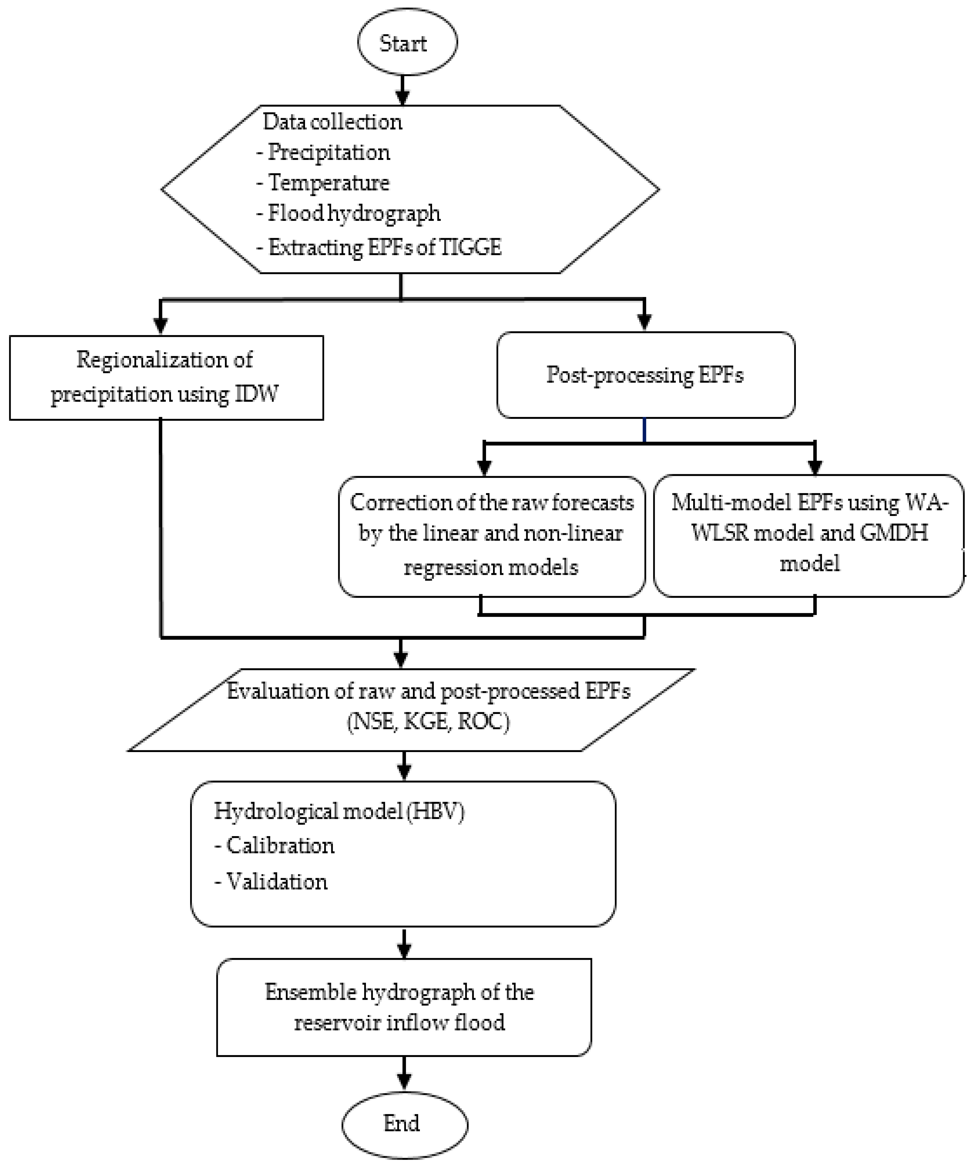
2.1. Research Methodology

In the present research, the NWP models were employed to quantify the uncertainty of precipitation forecasts. Figure 1 shows the research methodology flowchart. The recorded data from hydrometric and meteorological stations was collected to simulate ensemble inflow. The ensemble precipitation forecasts of the three meteorological models (NCEP, UKMO, and KMA) were extracted for six historical precipitation events that caused heavy floods. Then, the raw forecasts of the NWP models were compared with the observed precipitation. In order to improve the forecast skill of the NWP models, post-processing of the precipitation forecasts was carried out in two stages. In the first step, linear and nonlinear regression models were fitted between observed precipitation and the ensemble-mean of each single NWP model. The superior regression model was determined based on the values of goodness-of-fit metrics for both training and testing stages, and it was employed for the initial correction of all ensemble members. In the second step, corrected ensemble precipitation forecasts were merged using the GMDH model and WA-WLSR model to construct a multi-model ensemble system. Finally, a comparative evaluation was conducted for two modeling approaches containing deterministic forecasts (inflow forecasting by observed precipitation data) and ensemble forecasts (inflow forecasting by post-processed ensemble precipitation) to simulate ensemble reservoir inflow using the HBV model.

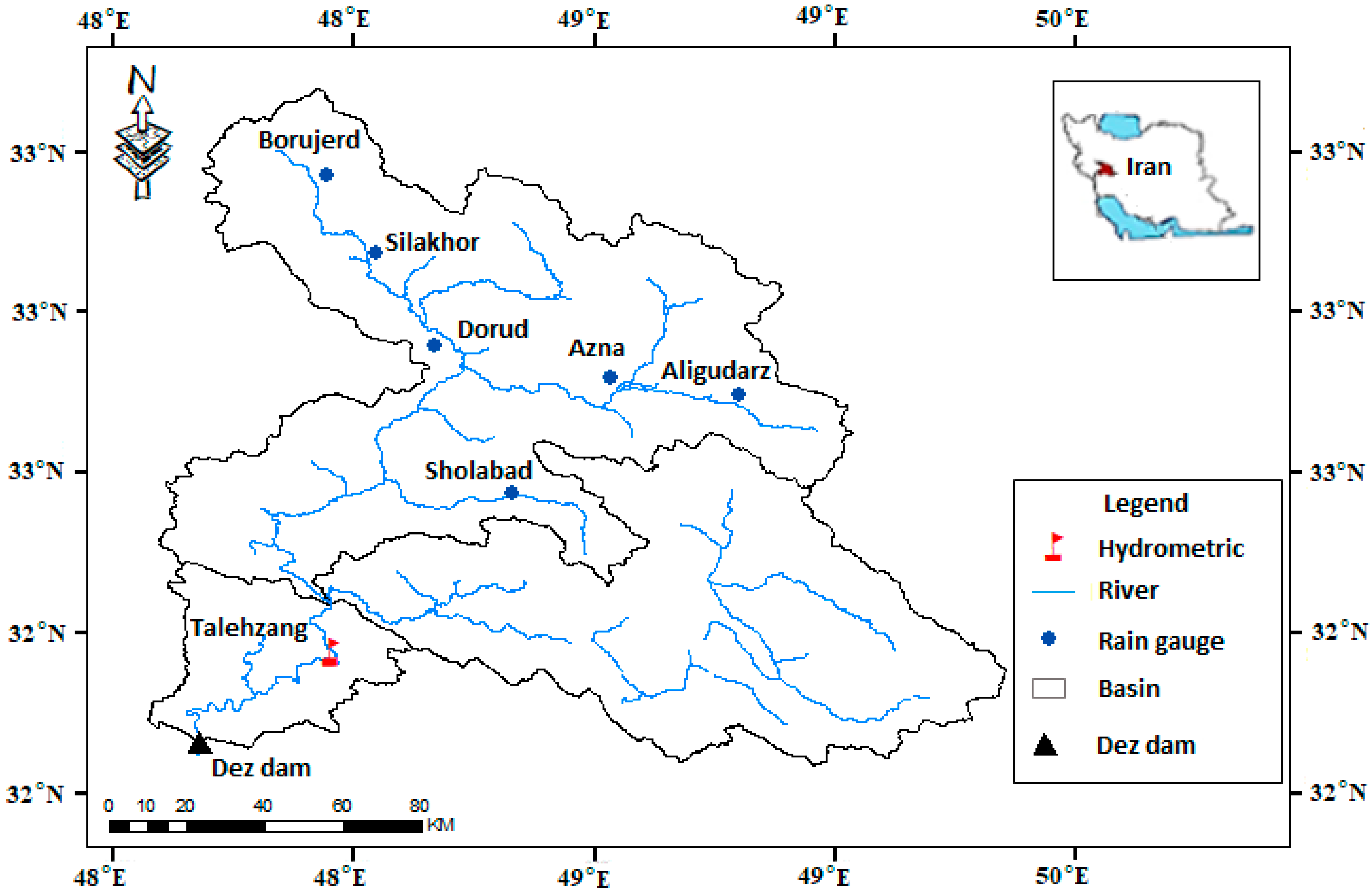
2.2. Case Study and Data

A multi-purpose Dez Dam reservoir has been selected as a study area to forecast ensemble inflow. The Dez River basin is located in southwest Iran at a latitude of 32°35′ N to 34°07′ N and a longitude of 48°20′ E to 50°20′ E. It is one of the main sub-basins of the Karun River and connects the Bakhtiari and Sezar Rivers. The Dez reservoir aims to supply domestic and agricultural water, control floods, and produce hydropower [37]. Figure 2 shows the location of the Dez basin, a hydrometric station, and synoptic rainfall stations. The basin area is 16213 km2, the average height is 1976 m, and the long-term mean annual rainfall is 784 mm. The flow data from the Taleh-Zang hydrometric station, located upstream of the reservoir, was applied to forecast ensemble inflow into the reservoir [37]. Over the past several decades, flood occurrence in the study area has caused huge damage [38]. Accordingly, six flood events were selected during 2013–2019. Table 1 illustrates the peak discharge during flood events, cumulative precipitation, and duration of the events. It is worth noting that these events were selected based on the date of the annual peak discharge.
Ensemble forecasts of the three NWP models (NCEP, UKMO, and KMA) were extracted from the THORPEX Interactive Grand Global Ensemble (TIGGE) database with the spatial resolution of 0.5 ° × 0.5 ° and 1-day lead time for precipitation events that caused floods [35,39]. The NCEP meteorological center is in Maryland, the United States. The source of the UKMO meteorological model is in Devon, United Kingdom. Besides, Seoul, South Korea, serves as the KMA meteorological model’s primary data source. The characteristics of the NWP models used in this research are presented in Table 2. Precipitation forecasts are updated with time intervals of six hours (00, 06, 12, and 18) in this database. The nearest neighbor interpolation method was applied to allocate the values of forecasted precipitation to the rain gauges [39]. The synoptic rainfall stations shown in Figure 2 contained complete data, and observed precipitation was used to evaluate the validity of the ensemble precipitation forecasts.
The input data to the HBV hydrological model to simulate ensemble reservoir inflow are discharge, precipitation, temperature, and potential evapotranspiration (PET) at the daily time step. The IDW interpolation method was used to estimate precipitation data uniformly over the Dez basin [40]. The uniform temperature data were estimated throughout the basin using the interpolation between the temperature and the elevation of the synoptic stations [41]. The PET was estimated by the Lowry–Johnson’s method [41,42].

2.3. Post-Processing Ensemble Precipitation Forecasts

After extracting the ensemble precipitation forecasts, the power regression model (PRM) and linear regression model were employed for the initial correction of the ensemble forecasts as follows [23,43]:
P O = a P r b
P O = b + a P r
where P O and P r are the observed precipitation and raw precipitation forecasts, respectively, while a and b are the coefficients of regressive models.
The power and linear regression models were fitted separately between the ensemble-mean of each single NWP model (independent variable) and observed precipitation (dependent variable). The superior regression model was determined based on goodness-of-fit metrics and was applied to the post-processing of all ensemble members. It is worth noting that 70% of the data were randomly considered for the training stage and 30% for the testing stage [43].
In this research, corrected precipitation forecasts of the NWP models were integrated using the GMDH model and WA-WLSR model to construct a grand ensemble system. The integration of the NWP models forecasts was carried out member by member. Accordingly, each member of the multi-model ensemble system was composed of a combination of NWP models’ members. The multi-model ensemble system comprised 20 members overall. The structure of the GMDH and WA-WLSR models is described in the following.

2.3.1. Multi-Model Ensemble System by the WA-WLSR Model

According to this approach, the corrected ensemble precipitation forecasts of NWP models were combined member by member using a weighted average model [17,44]. In this way, each member of the multi-model ensemble system has been obtained based on the weighted average of the three used NWP models [45]. The weighted average was calculated using the following equation:
P ¯ w = i = 1 N p f i w i i = 1 N w i
where P ¯ w is the weighted average of ensemble precipitation forecasts for all NWP models used in this research, N is the number of NWP models which is equal to 3, p f i is the ensemble precipitation forecasts of NWP models, and w i is the weight of each member for the NWP models.
The WLSR model was employed to estimate the weights in Equation (3). The WLSR is an efficient way to analyze small precipitation datasets for hydrological applications [46]. If y i = b + a x i represents the WLSR model, it minimizes the weighted sum-of-squared-error based on the following equation [46]:
L S = i = 1 n w i ( y i - a x i - b ) 2 i = 1 n w i
From which the parameters a and b are obtained as:
a = i = 1 n w i x i y i - i = 1 n w i x i i = 1 n w i y i w i i = 1 n w i x i 2 - ( i = 1 n w i x i ) 2 w i
b = i = 1 n w i y i - a i = 1 n w i x i w i
where w i is the weight of the i t h observation in the WLSR model [46].
In reality, the regression coefficients of the WLS model with a zero intercept were used as the weights in Equation (3). The weights have been estimated for each member separately so that the more precise observation (ensemble precipitation forecast) is given greater weight and vice versa [47].

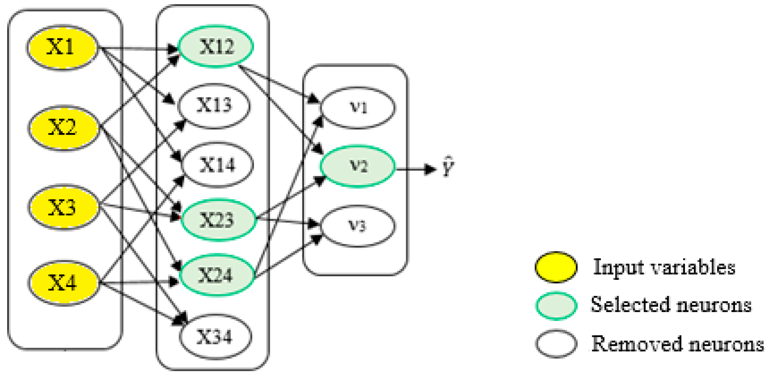
2.3.2. Multi-Model Ensemble System by the GMDH Model

GMDH is a subset of inductive deep-learning models that creates the relationship between input–output variables for a complex system using binomial functions as a feed-forward multilayer network [48]. This model adopts the Kolmogorov–Gabor polynomial to estimate the output variable ( Y ) based on the input dataset as follows:
Y = a 0 + i = 1 n a i x i + i = 1 n j = 1 n a i j x i x j + i = 1 n j = 1 n k = 1 n a i j k x i x j x k +
where X = ( x 1 , x 2 , , x n ) is the vector of input variables and A = ( a 1 , a 2 , , a n ) is the vector of coefficients [49]. The general structure of this algorithm is that all input variables are selected as neurons in the first layer. In the second layer, all possible bivariate combinations between the input variables in the first layer are generated and compared together to obtain the best possible fit for the output variable (Figure 3). In general, if we have N input variables, it will generate N ( N - 1 ) / 2 neurons at the next layers. Each neuron consists of two input variables, e.g., x 1 and x 2 , and employs the partial polynomial equation to estimate the output variable as:
Y = a 0 + a 1 x 1 + a 2 x 2 + a 3 x 1 2 + a 4 x 2 2 + a 5 x 1 x 2
where the coefficients { a 0 , , a 5 } are unknown and are estimated using the least squares method [50]. Therefore, as the number of layers, and subsequently neurons, increases, the model gradually becomes more complex. Consequently, a self-selection threshold is used in each layer to filter out neurons that do not contribute to the estimate of the output variable. The neurons that have better predictability than the previous generation are allowed to be transferred to the next layer. Then, the best result of the present layer is compared with the previous layer. If the results do not improve, the process will be stopped [50,51].
In this research, ensemble precipitation forecasts and observed precipitation were applied as input and output variables, respectively. For each member, 70% of the dataset was used for the training model, and the remaining 30% was applied to the testing model. Since this model separates the information into efficient and inefficient parts to estimate the output variable, it is more accurate than the neural network model. For this reason, the GMDH model has been employed in the current research.

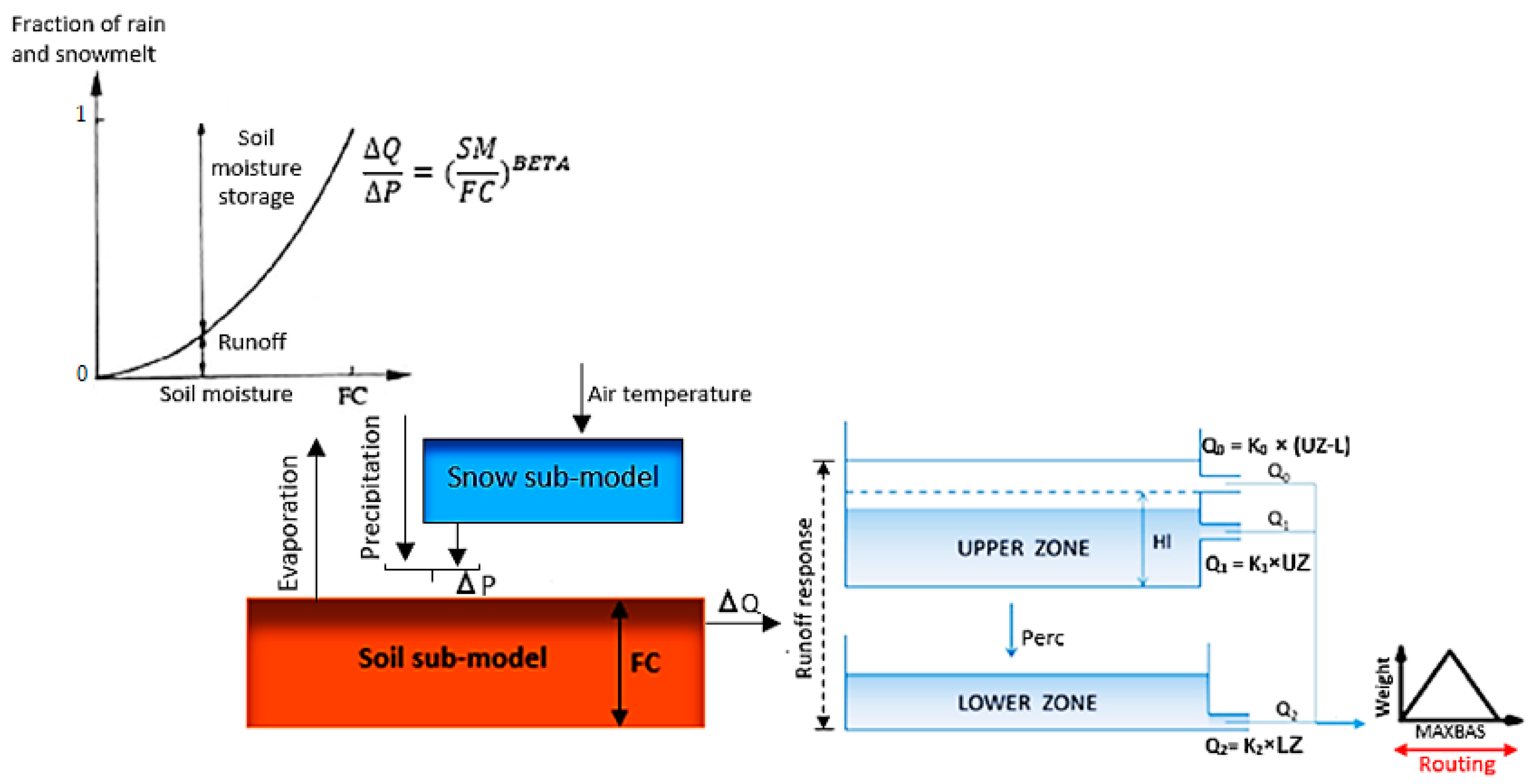
2.4. HBV Hydrological Model

The HBV hydrological model was set up to simulate ensemble reservoir inflow under two modelling approaches involving a deterministic forecast and an ensemble forecast. A deterministic forecast refers to a forecast based on observed precipitation data, while an ensemble forecast denotes a forecast based on post-processed ensemble precipitation data. The HBV model consists of three sub-models: snow accumulation and melt, soil moisture, and runoff response (Figure 4). This model calculates runoff based on precipitation ( P ), soil moisture ( S M ), field capacity ( F C ), and empirical coefficient ( B E T A ) that determines the relative contribution of runoff caused by snowmelt and precipitation (see the upper left side of Figure 4). The runoff is converted into discharge at the basin outlet by the runoff response sub-model. The runoff response is made of two storage zones. The upper zone has two outlets (Q0 and Q1), while the lower zone has only one outlet (Q2). These zones are coupled together by constant percolation (perc). After the water level exceeds a threshold limit (L) in the upper zone, runoff is rapidly triggered at the upper part of the upper zone (Q0). The parameters K0, K1, and K2 are used to control runoff associated with the response functions of the upper and lower zones [52]. The HBV model applies the triangular weight function (MAXBAS) which is used for routing the runoff at the outlet [52,53]. The HBV model’s parameters and their range are shown in Table 3.
The model calibration was carried out using the Harmony search automatic optimization method, which was suggested by Valent et al. (2012) and implemented in MATLAB [54]. Maximizing NSE was used as an objective function and for quantifying the goodness-of-fit between simulated and observed discharges [55].

2.5. Goodness-of-Fit Metrics

The goodness-of-fit metrics used in this research are presented in Table 4 [33]. They were employed to evaluate the validity of post-processed precipitation and inflow forecasts compared with the observed data.
Moreover, to investigate the hydrological model performance, a statistical framework introduced by Hossain et al. [56] was employed. Similar categorization can be found in the literature [57,58] which classifies the goodness-of-fit metrics into four distinct performance categories as shown in Table 5.
In addition to the criteria listed above, the relative operating characteristic (ROC) curve was applied to assess the discrimination power of probabilistic forecasts with respect to categorized precipitation observations, such as precipitation greater or smaller than a certain threshold [59]. In general, if the amount of precipitation exceeds the specific threshold, it can be said that the precipitation event has occurred. Otherwise, the precipitation event has not occurred. In order to produce an ROC diagram, the total number of data points ( N ) can be divided into two subsets: occurrence and non-occurrence ( N = O + O ). According to Table 6, H is the number of hits whenever the event has occurred and the alarm has been issued. FA is a false alarm, whenever the alarm has been issued, but no event has occurred. MA is a missed alarm, which indicates the number of times an event has occurred, but no alarm has been issued. CN is the correct no-alarm, which is the number of times that an event has not occurred and no alarm has been issued [59]. Bearing this in mind, the hit rate is defined as the number of occurred events that were correctly predicted ( H R = H / O ). The false alarm rate implies the number of events predicted that did not occur in reality ( F A R = F A / O ). Thus, the ROC curve is obtained by plotting the hit rate values against the false alarm rate. The greater the distance of the curve from the line 45°, the greater the forecast discrimination ability. In this research, the ROC diagram has been drawn for two precipitation thresholds, including 2.5 and 10 mm, which, respectively, represent the thresholds of light and heavy precipitation [60].

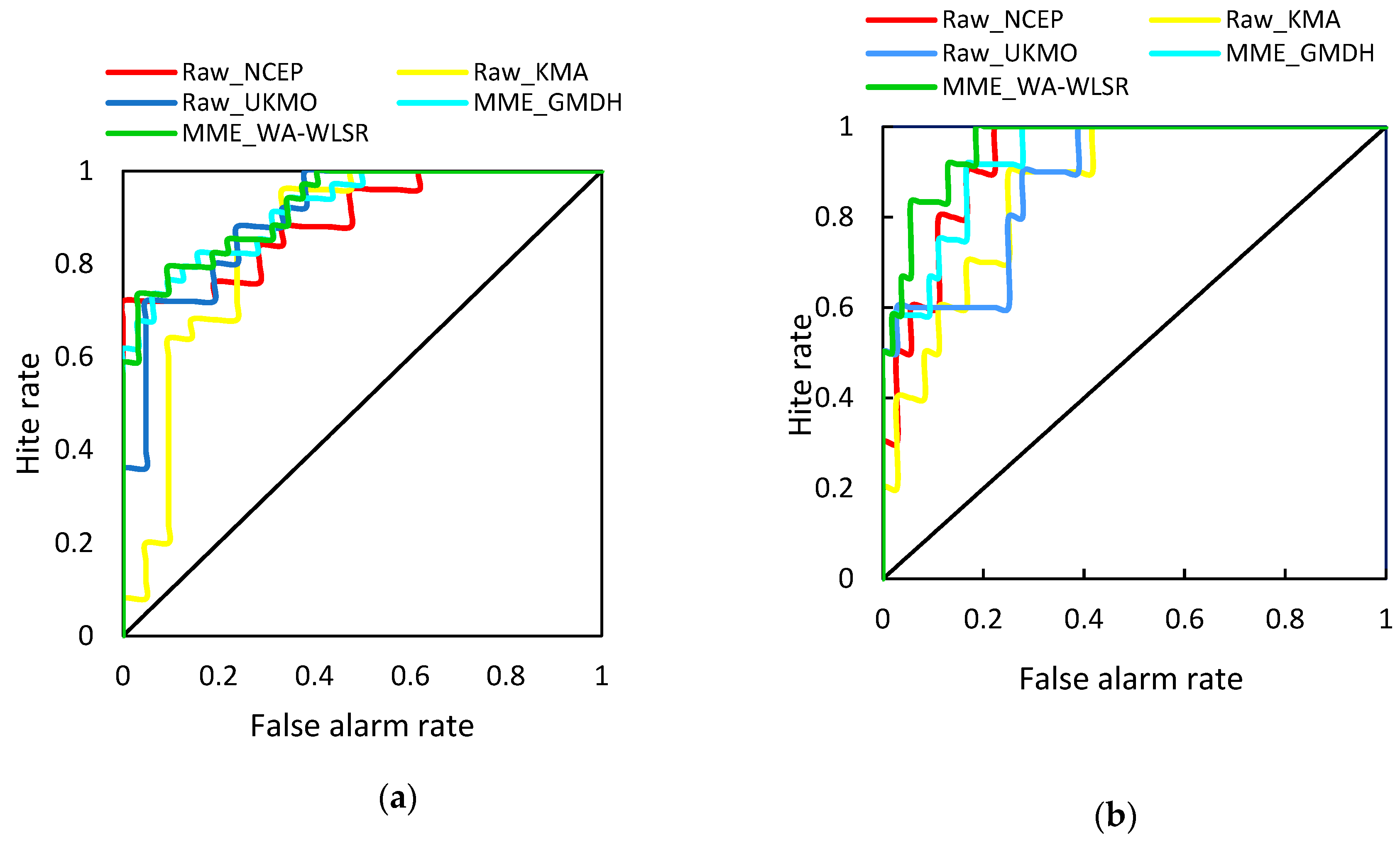
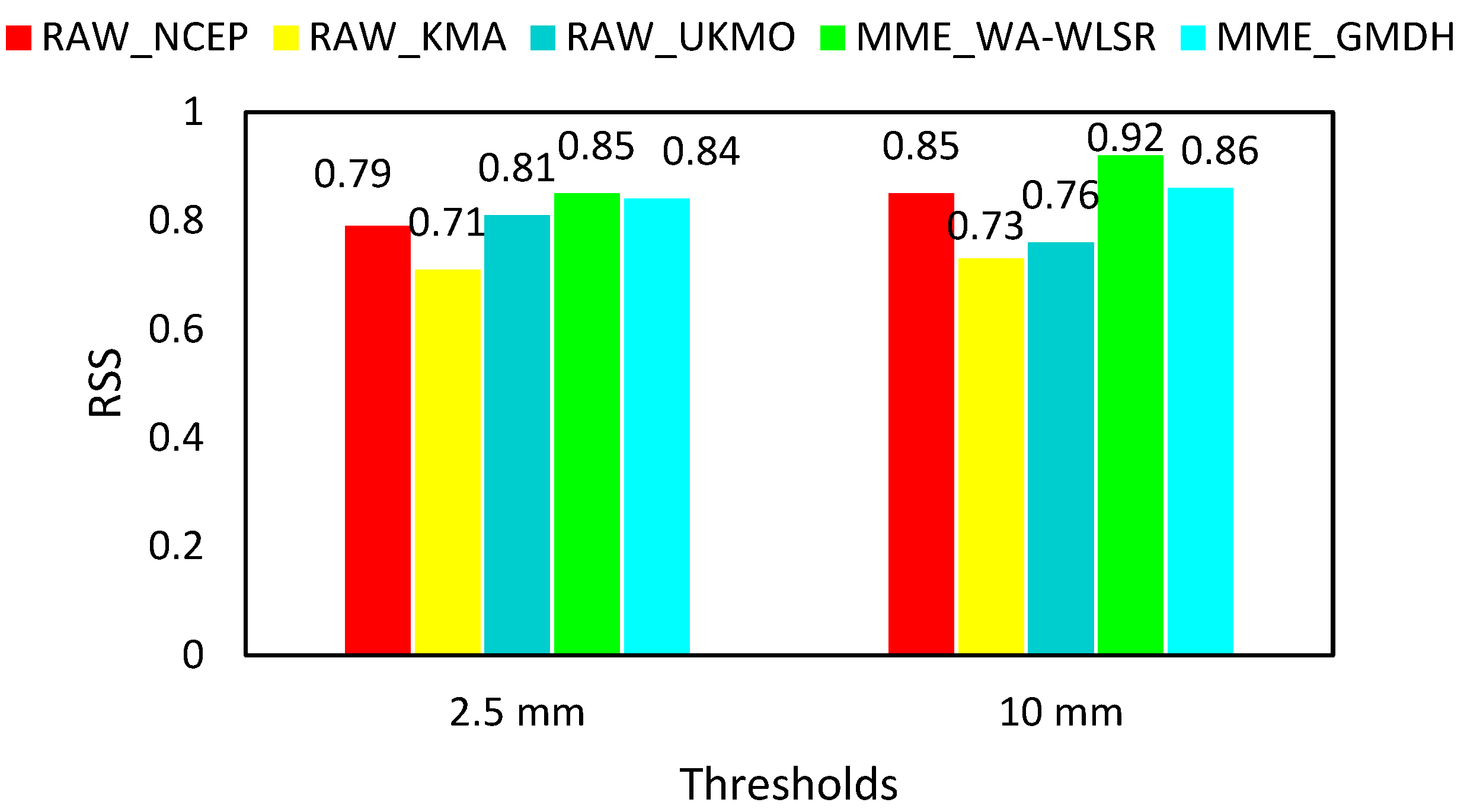
3. Results and Discussion

This part first presents the results of post-processing the raw output of the NWP models using linear and nonlinear regression models. In the next step, multi-model ensemble systems developed by GMDH and WA-WLSR models will be evaluated using goodness-of-fit metrics. Finally, we investigate the effectiveness of the HBV model to simulate the ensemble reservoir inflow using deterministic and probabilistic precipitation forecasts.

3.1. Correction of Ensemble Precipitation Forecasts

Regression models were employed to correct the raw forecasts of the NWP models. Table 6 and Table 7 display the outcomes of employing linear and nonlinear regression models to post-process the raw output of the NWP models. For each NWP model, regression models were separately fitted between the observed precipitation and the average of all ensemble members. The results were assessed based on Nash–Sutcliffe (NSE) and mean absolute error (MAE) criteria in both training and testing stages. The total number of data points is 66. The range of precipitation data for the training and testing stages is 33.92 and 14.43, respectively. According to a comparison of the goodness-of-fit metrics values in Table 7 and Table 8, the power regression models are slightly better than the linear regression models. In general, since power regression models have smaller average errors than linear models, they were utilized to post-process and correct all ensemble members of NWP models in this research.
The results of the post-processed forecasts were compared with the raw forecasts in Table 9 in order to investigate the effect of post-processing NWP models on enhancing the forecast skills of these models using power models. Additionally, this table shows the percentage of variations in improving the results of post-processed data in comparison with raw data for each NWP model individually. The results revealed that post-processed data indicated a superior forecast skill than the raw output of NWP models based on all goodness-of-fit metrics. Considering the values of goodness-of-fit metrics, more accurate results have been obtained using the NCEP and UKMO models, respectively. Given that the UKMO model has the highest percentage of variations based on the majority of goodness-of-fit metrics, it can be inferred that the improvement in results is more perceptible for the UKMO model compared with other models. It is worth noting that since more precise results were obtained using corrected ensemble precipitation data, the multi-model ensemble systems were developed based on post-processed ensemble precipitation forecasts derived from power regression models.

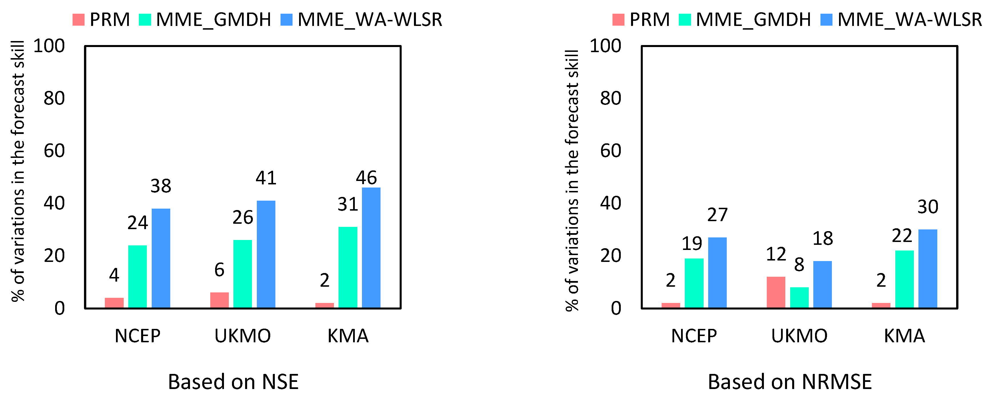
3.2. Multi-Model Ensemble Forecasts

In this research, in order to address the uncertainty caused by initial conditions and model structure, the output of the NWP models has been integrated [4,61,62]. Accordingly, a single forecast is produced based on the set of NWP models used in this research, and a multi-model ensemble system is created [61,63]. In the current research, the GMDH and WA-WLSR models were developed to combine ensemble precipitation forecasts. The results of multi-model ensemble forecasts for the GMDH model and WA-WLSR approach are presented in Table 10.
The results presented in Table 8 illustrate that the application of the GMDH and WA-WLSR models considerably enhances the ability of NWP models to forecast observed precipitation. According to Table 7 and Table 8, the forecast skill of NWP models has been significantly improved using multi-model ensemble systems rather than post-processing each individual model. For instance, in comparison with the power regression model, the values of the NSE and NRMSE metrics were improved on average for the GMDH model by 27% and 16%, and for the WA-WLSR model by 41% and 25%, respectively. These results are consistent with the results of previous studies [29,61,64,65]. Therefore, more accurate results derived from the proposed multi-model ensemble systems represent their efficiency in forecasting observed precipitation.
Figure 5 shows the percentage of variations in improving the forecast skill of the NWP models based on different approaches to post-processing raw outputs of ensemble forecasts using the NSE and NRMSE measures. This figure shows that the percentage of improvement in the forecasting ability of meteorological models for the power regression model is negligible compared with the multi-model approach. On the other hand, although both the WA-WLSR and GMDH models have a great impact on improving the forecasting skill of meteorological models, the WA-WLSR model is more efficient. As a result, adding a weak model can be effective in improving multiple models’ forecast skill and reducing their average error to the point where a single model cannot provide the same efficiency as the multi-model. Therefore, it can be expected that multi-model ensemble systems act as a reliable alternative for individual models.
The ROC diagram was employed to assess the discrimination capability of the NWP models. As it was mentioned, the ROC diagram depicts the hit rate versus the false alarm rate. Figure 6 shows the ROC diagram for the raw output of individual NWP models and multi-model ensemble systems. These curves have been drawn for two precipitation thresholds, 2.5 mm and 10 mm, which, respectively, represent the light precipitation threshold and heavy precipitation threshold. According to this figure, the ROC diagram corresponding to the multi-model ensemble system created by the WA-WLSR model (MME_WA-WLSR) is superior to that of other models based on evaluated precipitation thresholds. This implies that the discrimination ability of the WA-WLSR model is greater than that of individual NWP models for light and heavy precipitation thresholds. In general, the application of multi-model ensemble forecasts is beneficial for identifying both light and heavy precipitation.
The ROC Skill Score (RSS) index was utilized in order to assess the performance of ensemble precipitation forecasts based on the area under the ROC curve [66]. The RSS is calculated based on Equation (9).
R S S = 2 × ( A U C - 0.5 )
where in this equation A U C is the area under the ROC curve.
The numerical value of this index is between zero and one. The greater the area under the ROC curve, the closer the value of RSS index is to one, and the greater the forecast discrimination ability. The values of this index are presented in Figure 7 for before and after post-processing precipitation at the thresholds of 2.5 mm and 10 mm. The significant point demonstrated by Figure 7 is the fact that the identification skill of light and heavy precipitation events is increased using multi-model ensemble systems. Between the two proposed approaches for multi-model ensemble systems, the WA-WLSR model has a higher capacity than the GMDH model to identify light and heavy precipitation events. These results are compatible with those reported by Javanshiri et al. 2021. They improved the quality of WRF ensemble forecasts using the ensemble model output statistics (EMOS) and BMA approaches. The results of their research revealed that post-processing the WRF ensemble forecasts is effective in increasing the value of the RSS index and, consequently, improving the recognition skill of precipitation events, especially heavy precipitation events [67]. Therefore, the results clarified that combining the NWP models’ outputs using the WA-WLSR model provides robust results for recognizing precipitation events.
Figure 8 illustrates the scatter plots of raw and post-processed ensemble precipitation forecasts versus observed precipitation. The post-processed ensemble precipitation forecasts have a more appropriate dispersion around the 45° line than raw forecasts. It reveals that post-processed ensemble precipitation forecasts made by the GMDH and WA-WLSR models have superior quality. In addition, all used models overestimate light precipitation and underestimate heavy precipitation, whereas multi-model ensemble systems have lower overestimations and underestimations. Consequently, post-processed forecasts, especially in the case of the WA-WLSR model, closely match that of the observed precipitation.

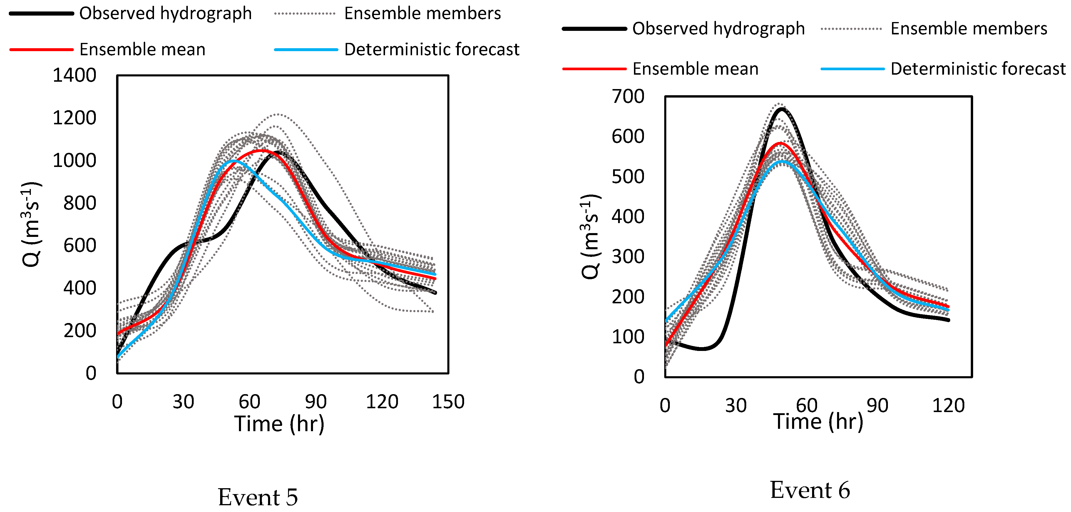
3.3. Ensemble Reservoir Inflow Forecasting

Ensemble hydrographs of the reservoir inflow were produced using post-processed ensemble precipitation forecasts derived from the WA-WLSR. Figure 9 indicates the results of the HBV model’s performance to simulate the ensemble reservoir inflow for the calibration stage. In this figure, hydrographs show observed inflow (black curve), the deterministic forecast simulated by observed precipitation (blue curve), ensemble forecasts including all ensemble members (grey curve), and the ensemble-mean of 20 members (red curve). The purpose of this visual examination of hydrographs is to highlight the fact that the HBV model performance is improved using hydrographs derived from post-processed ensemble precipitation forecasts. As it can be seen, there is a good agreement between the variations in pattern of observed inflow and simulated ensemble reservoir inflow in terms of rising limb, falling limb, and peak flow. In the majority of cases, the peak flows were underestimated using ensemble forecasts for different flood events. The comparison of ensemble inflow forecasts and deterministic inflow forecasts shows that deterministic inflow forecasts cannot reflect and quantify the uncertainty of the reservoir inflow, while it is crucial for reservoir operation in flood conditions to have knowledge concerning the range of reservoir inflow uncertainty before a flood occurrence. Generally, results revealed that ensemble reservoir inflow, in addition to addressing the uncertainty of the inflow forecasts, has a positive effect on the efficiency of the hydrological models.
Table 11 illustrates the goodness-of-fit metrics of the HBV model to simulate reservoir inflow hydrographs at the calibration stage for each flood event. The HBV model efficiency for a deterministic forecast and ensemble forecast (all ensemble members and ensemble-mean) was compared in this table. A deterministic forecast was simulated using observed precipitation derived from rain gauges, and an ensemble forecast was obtained by post-processed ensemble precipitation forecasts. The evaluation of model performance based on the NSE index revealed that the model efficiency for ensemble members and ensemble-mean was improved on average by 3% and 8%, respectively, in comparison with deterministic forecast for all flood events. Moreover, the values of the error index for ensemble members and ensemble-mean were decreased on average by 21% and 35%, respectively, compared with the deterministic forecast. Similar results were reported by Ye et al. [68]. They predicted flood events using a coupled atmospheric–hydrological modeling system based on ensemble forecasts and indicated that ensemble flood forecasting is a promising method due to its ability to provide more important information and risk probabilities than deterministic forecasting [68]. In another study, Ahmed [69] carried out a comparative analysis between ensemble inflow forecasts and deterministic forecasts. Results indicated that ensemble forecasts significantly enhance the hydrological model’s performance [69]. These results are in agreement with the results of previous research on ensemble streamflow/flood forecasting [35,36,39,70,71,72]. Therefore, the results indicate that post-processed ensemble precipitation forecasts has outperformed the HBV model effectiveness to simulate the reservoir inflow hydrograph.
According to the statistical framework proposed by Hossain et al. [56], the model’s performance level for the first three flood events can be considered “very good” in terms of the NSE, KGE, and MARE scores based on both modeling approaches (deterministic and ensemble forecasts). For the case of event 4, the model efficiency is at a “good” level in terms of the NSE and KGE scores (NSE, KGE > 0.65). Furthermore, the model’s performance is “acceptable” according to the MARE score. Generally, it can be said that the HBV model has a good ability to simulate ensemble reservoir inflow during the calibration period.
The validity of the HBV model was investigated using two flood events. Figure 10 shows the result of the HBV model to simulate ensemble reservoir inflow in the validation stage. As it can be seen, the variations’ trend of the observed hydrographs is approximately consistent with the forecasted hydrographs for both the ensemble forecast and deterministic forecast, while the spread of ensemble members increases to forecast peak discharge. The greater the dispersion of the ensemble members, the more uncertain the flow forecast. In other words, the HBV model’s error has been increased to forecast peak discharge at the validation stage. According to the results of the previous studies, precipitation, as one of the key climate variables, has a substantial impact on the flow forecast [73,74]. As a result, it can be found that the error caused by the NWP models in forecasting precipitation has affected the performance of the HBV hydrological model. In general, visual inspection of the HBV model at the validation stage revealed an approximate consistency between the forecasted and observed inflow hydrographs.
Table 12 indicates the goodness-of-fit metrics for the HBV model at the validation stage. The results demonstrate that when post-processed ensemble precipitation forecasts are employed for reservoir inflow simulation by the HBV model, the NSE values are enhanced for all ensemble members and the ensemble-mean by an average of 5% and 16%, respectively, compared with the deterministic forecasts. In addition, the average values of MARE for all ensemble members and the ensemble-mean are decreased by 2% and 12%, respectively, in comparison with deterministic forecasts. Therefore, it can be asserted that the use of post-processed ensemble precipitation forecasts is effective in increasing the HBV model’s efficiency for reservoir inflow forecasts based on all goodness-of-fit metrics.
Based on the statistical framework used in this research, since the values of goodness-of-fit metrics at the validation stage vary from one member to another, allocating one grade (good or satisfactory) to all members based on an average score may be ambiguous. Hence, it was decided to evaluate the model’s performance distribution over the members. For instance, Figure 11 indicates the NSE and MARE metrics for events 5 and 6, respectively. It is obviously observed from Figure 11a that while the model’s performance in terms of the NSE score was satisfactory for over 55% of the members in event 5, it gave a good level of performance for over 50% of the members in event 6. Based on Figure 11b, it is clear that the model performance is at a top level due to maintaining a “very good” grade for over 90% of members in event 5 and a “good” grade for over 70% of members in event 6.

4. Conclusions

Quantifying the uncertainty of precipitation forecasts using ensemble approaches is becoming increasingly important for flood forecasts and other practical purposes. The research’s main contribution is focused on evaluating the potential of post-processed ensemble precipitation forecasts to provide skillful ensemble reservoir inflow. In this regard, the raw forecasts of three NWP models were corrected through power regression models. Then, multi-model ensemble systems were developed using the GMDH and WA-WLSR models. Thereupon, post-processed ensemble precipitation is fed into the HBV hydrological model to produce as ensemble reservoir inflow forecast.
The findings of this research revealed that the accuracy of the precipitation forecast is somewhat improved by the initial correction of the raw forecasts of each NWP model using the power regression models, but the amount of improvement in the forecasting skill of these models was more perceptible with the construction of the multi-model ensemble systems. For instance, compared with the power regression model, the average values of the NSE and NRMSE measures were improved by 27% and 16% for the GMDH model and by 41% and 25% for the WA-WLSR model, respectively. The results of simulating ensemble reservoir inflow using the HBV model indicated that the average percentage of error for the cases of all ensemble members and the ensemble-mean was decreased by 2% and 12%, respectively, compared with the deterministic forecasts at the validation stage. It represented that post-processed ensemble precipitation forecasts had a remarkable impact on the quality of the forecast using the HBV model. The improvement of results for ensemble forecasts was also revealed by a visual investigation of scatter plots, hydrographs of ensemble members and the ensemble-mean. Based on the statistical framework used in this research for investigating the hydrological model’s performance, the results revealed that the model’s performance is at a “good” level for the majority of flood events.
The results of this research emphasize the advantage of post-processing ensemble precipitation forecasts before their application as input to the hydrological models for flood forecasting and warning, reservoir inflow, river flow, and water resources management.

Author Contributions

Design the research, J.S., M.T.; collection of observed data, S.L.; formal analysis, M.T.; methodology, K.H., S.K. and M.T.; writing original draft, M.T.; providing critical points for further improvement of manuscript, K.H., J.S.; writing review and editing, S.K., B.M. and Z.P. Funding acquisition, K.H., S.K. and Z.P. All authors have read and agreed to the published version of the manuscript.

Funding

This work was supported by the Slovak Research and Development Agency under Contract No. APVV 19-0340, No. APVV 20-0374 and the VEGA Grant Agency No. VEGA 1/0632/19.

Data Availability Statement

Ensemble precipitation data derived from http://apps.ecmwf.int/datasets/data/tigge/levtype=sfc/type=pf/, accessed on 24 February 2023). Precipitation, temperature, and flood hydrograph data were collected from Iran Water Resources Management Company (https://www.wrm.ir/, accessed on 24 February 2023).

Acknowledgments

We sincerely thank the editor and two reviewers for their helpful comments, which significantly improved the quality of the manuscript.

Conflicts of Interest

The authors declare no conflict of interest.

References

  1. Li, Y.; Xu, B.; Wang, D.; Wang, Q.; Zheng, X.; Xu, J.; Zhou, F.; Huang, H.; Xu, Y. Deterministic and probabilistic evaluation of raw and post-processing monthly precipitation forecasts: A case study of China. J. Hydroinform. 2021, 23, 914–934. [Google Scholar] [CrossRef]
  2. Wu, L.; Seo, D.-J.; Demargne, J.; Brown, J.D.; Cong, S.; Schaake, J. Generation of ensemble precipitation forecast from single-valued quantitative precipitation forecast for hydrologic ensemble prediction. J. Hydrol. 2011, 399, 281–298. [Google Scholar] [CrossRef]
  3. Cloke, H.; Pappenberger, F. Ensemble flood forecasting: A review. J. Hydrol. 2009, 375, 613–626. [Google Scholar] [CrossRef]
  4. Wu, J.; Lu, G.; Wu, Z. Flood forecasts based on multi-model ensemble precipitation forecasting using a coupled atmospheric-hydrological modeling system. Nat. Hazards 2014, 74, 325–340. [Google Scholar] [CrossRef]
  5. Banihabib, M.E.; Arabi, A. The impact of catchment management on emergency management of flash-flood. Int. J. Emerg. Manag. 2016, 12, 185–195. [Google Scholar] [CrossRef]
  6. Chang, M.-J.; Chang, H.-K.; Chen, Y.-C.; Lin, G.-F.; Chen, P.-A.; Lai, J.-S.; Tan, Y.-C. A support vector machine forecasting model for typhoon flood inundation mapping and early flood warning systems. Water 2018, 10, 1734. [Google Scholar] [CrossRef] [Green Version]
  7. Maddah, M.A.; Akhoond-Ali, A.M.; Ahmadi, F.; Ghafarian, P.; Rusin, I.N. Forecastability of a heavy precipitation event at different lead-times using WRF model: The case study in Karkheh River basin. Acta Geophys. 2021, 69, 1979–1995. [Google Scholar] [CrossRef]
  8. Nohara, D.; Nishioka, Y.; Hori, T.; Sato, Y. Real-time reservoir operation for flood management considering ensemble streamflow prediction and its uncertainty. In Advances in Hydroinformatics; Springer: Berlin/Heidelberg, Germany, 2016; pp. 333–347. [Google Scholar]
  9. Jain, S.K.; Mani, P.; Jain, S.K.; Prakash, P.; Singh, V.P.; Tullos, D.; Kumar, S.; Agarwal, S.; Dimri, A. A Brief review of flood forecasting techniques and their applications. Int. J. River Basin Manag. 2018, 16, 329–344. [Google Scholar] [CrossRef]
  10. Wu, W.; Emerton, R.; Duan, Q.; Wood, A.W.; Wetterhall, F.; Robertson, D.E. Ensemble flood forecasting: Current status and future opportunities. Wiley Interdiscip. Rev. Water 2020, 7, e1432. [Google Scholar] [CrossRef]
  11. Ahmad, S.K.; Hossain, F. Maximizing energy production from hydropower dams using short-term weather forecasts. Renew. Energy 2020, 146, 1560–1577. [Google Scholar] [CrossRef]
  12. Emerton, R.E.; Stephens, E.M.; Pappenberger, F.; Pagano, T.C.; Weerts, A.H.; Wood, A.W.; Salamon, P.; Brown, J.D.; Hjerdt, N.; Donnelly, C. Continental and global scale flood forecasting systems. Wiley Interdiscip. Rev. Water 2016, 3, 391–418. [Google Scholar] [CrossRef] [Green Version]
  13. Rani, S.I.; Sharma, P.; George, J.P.; Das Gupta, M. Assimilation of individual components of radiosonde winds: An investigation to assess the impact of single-component winds from space-borne measurements on NWP. J. Earth Syst. Sci. 2021, 130, 89. [Google Scholar] [CrossRef]
  14. Chen, G.; Hou, J.; Zhou, N.; Yang, S.; Tong, Y.; Su, F.; Huang, L.; Bi, X. High-Resolution Urban Flood Forecasting by Using a Coupled Atmospheric and Hydrodynamic Flood Models. Front. Earth Sci. 2020, 8, 545612. [Google Scholar] [CrossRef]
  15. Tian, J.; Liu, J.; Yan, D.; Ding, L.; Li, C. Ensemble flood forecasting based on a coupled atmospheric-hydrological modeling system with data assimilation. Atmos. Res. 2019, 224, 127–137. [Google Scholar] [CrossRef]
  16. Wu, Z.; Wu, J.; Lu, G. A one-way coupled atmospheric-hydrological modeling system with combination of high-resolution and ensemble precipitation forecasting. Front. Earth Sci. 2016, 10, 432–443. [Google Scholar] [CrossRef]
  17. Bourdin, D.R.; Stull, R.B. Bias-corrected short-range Member-to-Member ensemble forecasts of reservoir inflow. J. Hydrol. 2013, 502, 77–88. [Google Scholar] [CrossRef]
  18. Tao, Y.; Duan, Q.; Ye, A.; Gong, W.; Di, Z.; Xiao, M.; Hsu, K. An evaluation of post-processed TIGGE multimodel ensemble precipitation forecast in the Huai river basin. J. Hydrol. 2014, 519, 2890–2905. [Google Scholar] [CrossRef] [Green Version]
  19. Daoud, A.B.; Sauquet, E.; Bontron, G.; Obled, C.; Lang, M. Daily quantitative precipitation forecasts based on the analogue method: Improvements and application to a French large river basin. Atmos. Res. 2016, 169, 147–159. [Google Scholar] [CrossRef] [Green Version]
  20. Amini, S.; Azizian, A.; Daneshkar Arasteh, P. How reliable are TIGGE daily deterministic precipitation forecasts over different climate and topographic conditions of Iran? Meteorol. Appl. 2021, 28, e2013. [Google Scholar] [CrossRef]
  21. Flowerdew, J. Calibrating ensemble reliability whilst preserving spatial structure. Tellus A Dyn. Meteorol. Oceanogr. 2014, 66, 22662. [Google Scholar] [CrossRef] [Green Version]
  22. Piani, C.; Haerter, J.; Coppola, E. Statistical bias correction for daily precipitation in regional climate models over Europe. Theor. Appl. Climatol. 2010, 99, 187–192. [Google Scholar] [CrossRef] [Green Version]
  23. Du, Y.; Wang, Q.J.; Wu, W.; Yang, Q. Power transformation of variables for post-processing precipitation forecasts: Regionally versus locally optimized parameter values. J. Hydrol. 2022, 610, 127912. [Google Scholar] [CrossRef]
  24. Manzanas, R.; Gutiérrez, J.M.; Bhend, J.; Hemri, S.; Doblas-Reyes, F.J.; Torralba, V.; Penabad, E.; Brookshaw, A. Bias adjustment and ensemble recalibration methods for seasonal forecasting: A comprehensive intercomparison using the C3S dataset. Clim. Dyn. 2019, 53, 1287–1305. [Google Scholar] [CrossRef]
  25. Barnes, C.; Brierley, C.M.; Chandler, R.E. New approaches to postprocessing of multi-model ensemble forecasts. Q. J. R. Meteorol. Soc. 2019, 145, 3479–3498. [Google Scholar] [CrossRef]
  26. Palmer, T.N.; Alessandri, A.; Andersen, U.; Cantelaube, P.; Davey, M.; Delécluse, P.; Déqué, M.; Diez, E.; Doblas-Reyes, F.J.; Feddersen, H. Development of a European multimodel ensemble system for seasonal-to-interannual prediction (DEMETER). Bull. Am. Meteorol. Soc. 2004, 85, 853–872. [Google Scholar] [CrossRef] [Green Version]
  27. Wei, X.; Sun, X.; Sun, J.; Yin, J.; Sun, J.; Liu, C. A Comparative Study of Multi-Model Ensemble Forecasting Accuracy between Equal-and Variant-Weight Techniques. Atmosphere 2022, 13, 526. [Google Scholar] [CrossRef]
  28. Medina, H.; Tian, D.; Srivastava, P.; Pelosi, A.; Chirico, G.B. Medium-range reference evapotranspiration forecasts for the contiguous United States based on multi-model numerical weather predictions. J. Hydrol. 2018, 562, 502–517. [Google Scholar] [CrossRef]
  29. Pakdaman, M.; Babaeian, I.; Bouwer, L.M. Improved Monthly and Seasonal Multi-Model Ensemble Precipitation Forecasts in Southwest Asia Using Machine Learning Algorithms. Water 2022, 14, 2632. [Google Scholar] [CrossRef]
  30. Baran, S. Probabilistic wind speed forecasting using Bayesian model averaging with truncated normal components. Comput. Stat. Data Anal. 2014, 75, 227–238. [Google Scholar] [CrossRef] [Green Version]
  31. Han, K.; Choi, J.; Kim, C. Comparison of statistical post-processing methods for probabilistic wind speed forecasting. Asia-Pac. J. Atmos. Sci. 2018, 54, 91–101. [Google Scholar] [CrossRef]
  32. Lee, J.A.; Kolczynski, W.C.; McCandless, T.C.; Haupt, S.E. An objective methodology for configuring and down-selecting an NWP ensemble for low-level wind prediction. Mon. Weather Rev. 2012, 140, 2270–2286. [Google Scholar] [CrossRef]
  33. Saedi, A.; Saghafian, B.; Moazami, S.; Aminyavari, S. Performance evaluation of sub-daily ensemble precipitation forecasts. Meteorol. Appl. 2020, 27, e1872. [Google Scholar] [CrossRef] [Green Version]
  34. Wang, X.; Yang, T.; Li, X.; Shi, P.; Zhou, X. Spatio-temporal changes of precipitation and temperature over the Pearl River basin based on CMIP5 multi-model ensemble. Stoch. Environ. Res. Risk Assess. 2017, 31, 1077–1089. [Google Scholar] [CrossRef]
  35. Aminyavari, S.; Saghafian, B. Probabilistic streamflow forecast based on spatial post-processing of TIGGE precipitation forecasts. Stoch. Environ. Res. Risk Assess. 2019, 33, 1939–1950. [Google Scholar] [CrossRef]
  36. Yang, S.-C.; Yang, T.-H. Uncertainty assessment: Reservoir inflow forecasting with ensemble precipitation forecasts and HEC-HMS. Adv. Meteorol. 2014, 2014, 581756. [Google Scholar] [CrossRef] [Green Version]
  37. Banihabib, M.E.; Bandari, R.; Valipour, M. Improving daily peak flow forecasts using hybrid Fourier-series autoregressive integrated moving average and recurrent artificial neural network models. AI 2020, 1, 17. [Google Scholar] [CrossRef]
  38. Malekmohammadi, B.; Zahraie, B.; Kerachian, R. A real-time operation optimization model for flood management in river-reservoir systems. Nat. Hazards 2010, 53, 459–482. [Google Scholar] [CrossRef]
  39. Goodarzi, L.; Banihabib, M.E.; Roozbahani, A. A decision-making model for flood warning system based on ensemble forecasts. J. Hydrol. 2019, 573, 207–219. [Google Scholar] [CrossRef]
  40. Shope, C.L.; Maharjan, G.R. Modeling spatiotemporal precipitation: Effects of density, interpolation, and land use distribution. Adv. Meteorol. 2015, 2015, 174196. [Google Scholar] [CrossRef] [Green Version]
  41. Tanhapour, M.; Hlavčová, K.; Soltani, J.; Liová, A.; Malekmohammadi, B. Sensitivity analysis and assessment of the performance of the HBV hydrological model for simulating reservoir inflow hydrograph. In Proceedings of the 16th Annual International Scientific Conference, Science of Youth, Banská Štiavnica, Slovakia, 1–3 June 2022; pp. 115–124. [Google Scholar]
  42. Mazăre, R.; Borbely, L.; Ghenț, L.; Ienciu, A.; Manea, D. Studies on water requirements in corn crops under the conditions of Arad. Res. J. Agric. Sci. 2018, 50, 413–419. [Google Scholar]
  43. Theocharides, S.; Makrides, G.; Livera, A.; Theristis, M.; Kaimakis, P.; Georghiou, G.E. Day-ahead photovoltaic power production forecasting methodology based on machine learning and statistical post-processing. Appl. Energy 2020, 268, 115023. [Google Scholar] [CrossRef]
  44. Liao, W.; Lei, X. Multi-model Combination Techniques for Flood Forecasting from the Distributed Hydrological Model EasyDHM. In Proceedings of the International Symposium on Intelligence Computation and Applications, Wuhan, China, 27–28 October 2012; Springer: Berlin/Heidelberg, Germany, 2012; pp. 396–402. [Google Scholar]
  45. Fathi, M.; Azadi, M.; Kamali, G.; Meshkatee, A.H. Improving precipitation forecasts over Iran using a weighted average ensemble technique. J. Earth Syst. Sci. 2019, 128, 133. [Google Scholar] [CrossRef] [Green Version]
  46. Hughes, C.E.; Crawford, J. A new precipitation weighted method for determining the meteoric water line for hydrological applications demonstrated using Australian and global GNIP data. J. Hydrol. 2012, 464, 344–351. [Google Scholar] [CrossRef]
  47. Mutiu, O.S. Application of weighted least squares regression in forecasting. Int. J. Recent. Res. Interdiscip. Sci 2015, 2, 45–54. [Google Scholar]
  48. Dodangeh, E.; Panahi, M.; Rezaie, F.; Lee, S.; Bui, D.T.; Lee, C.-W.; Pradhan, B. Novel hybrid intelligence models for flood-susceptibility prediction: Meta optimization of the GMDH and SVR models with the genetic algorithm and harmony search. J. Hydrol. 2020, 590, 125423. [Google Scholar] [CrossRef]
  49. Adnan, R.M.; Liang, Z.; Parmar, K.S.; Soni, K.; Kisi, O. Modeling monthly streamflow in mountainous basin by MARS, GMDH-NN and DENFIS using hydroclimatic data. Neural Comput. Appl. 2021, 33, 2853–2871. [Google Scholar] [CrossRef]
  50. Shaghaghi, S.; Bonakdari, H.; Gholami, A.; Ebtehaj, I.; Zeinolabedini, M. Comparative analysis of GMDH neural network based on genetic algorithm and particle swarm optimization in stable channel design. Appl. Math. Comput. 2017, 313, 271–286. [Google Scholar] [CrossRef]
  51. Chang, F.J.; Hwang, Y.Y. A self-organization algorithm for real-time flood forecast. Hydrol. Process. 1999, 13, 123–138. [Google Scholar] [CrossRef]
  52. Parra, V.; Fuentes-Aguilera, P.; Muñoz, E. Identifying advantages and drawbacks of two hydrological models based on a sensitivity analysis: A study in two Chilean watersheds. Hydrol. Sci. J. 2018, 63, 1831–1843. [Google Scholar] [CrossRef]
  53. Parajka, J.; Merz, R.; Blöschl, G. Uncertainty and multiple objective calibration in regional water balance modelling: Case study in 320 Austrian catchments. Hydrol. Process. Int. J. 2007, 21, 435–446. [Google Scholar] [CrossRef]
  54. Valent, P.; Szolgay, J.; Riverso, C. Assessment of the uncertainties of a conceptual hydrologic model by using artificially generated flows. Slovak J. Civ. Eng. 2012, 20, 35. [Google Scholar] [CrossRef]
  55. Nash, J.E.; Sutcliffe, J.V. River flow forecasting through conceptual models part I—A discussion of principles. J. Hydrol. 1970, 10, 282–290. [Google Scholar] [CrossRef]
  56. Hossain, S.; Hewa, G.A.; Wella-Hewage, S. A comparison of continuous and event-based rainfall–runoff (RR) modelling using EPA-SWMM. Water 2019, 11, 611. [Google Scholar] [CrossRef] [Green Version]
  57. Moriasi, D.; Wilson, B.; Douglas-Mankin, K.; Arnold, J.; Gowda, P. Hydrologic and water quality models: Use, calibration, and validation. Trans. ASABE 2012, 55, 1241–1247. [Google Scholar] [CrossRef]
  58. Moriasi, D.N.; Gitau, M.W.; Pai, N.; Daggupati, P. Hydrologic and water quality models: Performance measures and evaluation criteria. Trans. ASABE 2015, 58, 1763–1785. [Google Scholar]
  59. D’onofrio, A.; Boulanger, J.-P.; Segura, E.C. CHAC: A weather pattern classification system for regional climate downscaling of daily precipitation. Clim. Chang. 2010, 98, 405–427. [Google Scholar] [CrossRef]
  60. Zakeri, Z.; Azadi, M.; Sahraeiyan, F. Verification of WRF forecasts for precipitation over Iran in the period Feb–May 2009. Nivar 2014, 38, 3–10. [Google Scholar]
  61. Hagedorn, R.; Doblas-Reyes, F.J.; Palmer, T.N. The rationale behind the success of multi-model ensembles in seasonal forecasting—I. Basic concept. Tellus A Dyn. Meteorol. Oceanogr. 2005, 57, 219–233. [Google Scholar]
  62. Ren, H.-L.; Wu, Y.; Bao, Q.; Ma, J.; Liu, C.; Wan, J.; Li, Q.; Wu, X.; Liu, Y.; Tian, B. The China multi-model ensemble prediction system and its application to flood-season prediction in 2018. J. Meteorol. Res. 2019, 33, 540–552. [Google Scholar] [CrossRef]
  63. Krishnamurti, T.; Sagadevan, A.; Chakraborty, A.; Mishra, A.; Simon, A. Improving multimodel weather forecast of monsoon rain over China using FSU superensemble. Adv. Atmos. Sci. 2009, 26, 813–839. [Google Scholar] [CrossRef]
  64. Davolio, S.; Miglietta, M.; Diomede, T.; Marsigli, C.; Morgillo, A.; Moscatello, A. A meteo-hydrological prediction system based on a multi-model approach for precipitation forecasting. Nat. Hazards Earth Syst. Sci. 2008, 8, 143–159. [Google Scholar] [CrossRef]
  65. Tang, Y.; Wu, Q.; Li, X.; Sun, Y.; Hu, C. Comparison of different ensemble precipitation forecast system evaluation, integration and hydrological applications. Acta Geophys. 2022, 71, 405–421. [Google Scholar] [CrossRef]
  66. Yin, J.; Hao, Y.; Samawi, H.; Rochani, H. Rank-based kernel estimation of the area under the ROC curve. Stat. Methodol. 2016, 32, 91–106. [Google Scholar] [CrossRef]
  67. Javanshiri, Z.; Fathi, M.; Mohammadi, S.A. Comparison of the BMA and EMOS statistical methods for probabilistic quantitative precipitation forecasting. Meteorol. Appl. 2021, 28, e1974. [Google Scholar] [CrossRef]
  68. Ye, J.; Shao, Y.; Li, Z. Flood forecasting based on TIGGE precipitation ensemble forecast. Adv. Meteorol. 2016, 2016, 9129734. [Google Scholar] [CrossRef] [Green Version]
  69. Ahmed, S. Hydrologic Ensemble Predictions Using Ensemble Meteorological Forecasts. Ph.D. thesis, McMaster Univercity, Hamilton, ON, Canada, 2010; p. 91. [Google Scholar]
  70. Ferretti, R.; Lombardi, A.; Tomassetti, B.; Sangelantoni, L.; Colaiuda, V.; Mazzarella, V.; Maiello, I.; Verdecchia, M.; Redaelli, G. Regional ensemble forecast for early warning system over small Apennine catchments on Central Italy. Hydrol. Earth Syst. Sci. Discuss 2019, 1–25. [Google Scholar] [CrossRef]
  71. Jie, W.; Wu, T.; Wang, J.; Li, W.; Polivka, T. Using a deterministic time-lagged ensemble forecast with a probabilistic threshold for improving 6–15 day summer precipitation prediction in China. Atmos. Res. 2015, 156, 142–159. [Google Scholar] [CrossRef] [Green Version]
  72. Wang, F.; Wang, L.; Zhou, H.; Saavedra Valeriano, O.C.; Koike, T.; Li, W. Ensemble hydrological prediction-based real-time optimization of a multiobjective reservoir during flood season in a semiarid basin with global numerical weather predictions. Water Resour. Res. 2012, 48, 1–21. [Google Scholar] [CrossRef]
  73. Ran, Q.; Fu, W.; Liu, Y.; Li, T.; Shi, K.; Sivakumar, B. Evaluation of quantitative precipitation predictions by ECMWF, CMA, and UKMO for flood forecasting: Application to two basins in China. Nat. Hazards Rev. 2018, 19, 1–13. [Google Scholar] [CrossRef] [Green Version]
  74. Yang, C.; Yuan, H.; Su, X. Bias correction of ensemble precipitation forecasts in the improvement of summer streamflow prediction skill. J. Hydrol. 2020, 588, 124955. [Google Scholar] [CrossRef]
Figure 1. Research methodology flowchart used for ensemble reservoir inflow forecast.
Water 15 00887 g001
Figure 2. The location of the Dez basin, rain gauges, and the hydrometric station.
Water 15 00887 g002
Figure 3. The structure of the GMDH model with four input variables.
Water 15 00887 g003
Figure 4. Schematic of the HBV model with main equations [41].
Water 15 00887 g004
Figure 5. The percentage of variations in improving the forecast skill of the NWP models based on post-processing approaches.
Water 15 00887 g005
Figure 6. ROC diagrams for raw and post-processed ensemble precipitation forecasts: (a) 2.5 mm (b) 10 mm.
Water 15 00887 g006
Figure 7. Comparison of RSS index for raw and post-processed ensemble precipitation forecasts.
Water 15 00887 g007
Figure 8. Scatter plots for raw and post-processed ensemble precipitation forecasts.
Water 15 00887 g008
Figure 9. Ensemble reservoir inflow during flood events for the calibration stage. Black lines: observed inflow hydrograph; blue lines: the deterministic inflow forecast based on observed precipitation; grey lines: ensemble inflow forecasts simulated by post-processed EPFs containing all ensemble members; red lines: ensemble-mean of all members.
Water 15 00887 g009
Figure 10. Ensemble reservoir inflow during flood events at the validation stage.
Water 15 00887 g010
Figure 11. Model’s performance distribution over the members of ensemble reservoir inflow at the validation stage based on (a) NSE and (b) MARE criteria.
Water 15 00887 g011
Table 1. Observed precipitation and streamflow data.
Event NoDate of EventsPeak Discharge (m3/s)Time (h)Precipitation Depth (mm)
129.01.20136334831.33
224.03.201713077237.93
325.02.20186227219.67
401.04.2019522248104.39
528.12.2016103784101.26
618.02.20186657248.8
Table 2. Characteristics of the NWP models used in this research.
CenterForecast Length (Day)Model Resolution (lon × lat)Number of Ensemble MembersBase Time (UTC)
NCEP161.00° × 1.00°2000/06/12/18
UKMO150.83° × 0.56°2300/12
KMA101.00° × 1.00°2400/12
Table 3. Description of the HBV model parameters along with their range.
Sub-ModelsParametersDescription of the ParametersRange
SnowTrTemperature threshold above which precipitation is liquid [°C]0–2
TsTemperature threshold below which precipitation is solid [°C]−2–0
TmTemperature threshold above which snowmelt starts [°C]−2–2
DDFDegree-day factor determines the speed of the snow melting [mm/°C/day]1–5
SCFFactor for correcting snow measurements [-]1–1.6
Soil moistureFCField capacity- maximum soil moisture storage [mm]100–250
LpA limit for potential evapotranspiration [-]0.5–1
BETACoefficient influencing the amount of water caused by soil moisture and the upper reservoir [-]0.1–2.5
Runoff responsepercConstant percolation rate from the upper to the bottom reservoir [mm]0.5–4
LThreshold storage state for initiating very fast surface runoff [mm]10–60
K0The recession coefficients associated with the surface (K0), sub-surface (K1), and base flow (K2) [-]1–5
K15–30
K230–120
MaxbasThe parameter for runoff routing [-]1–6
Table 4. Summary of goodness-of-fit metrics used in this research.
Goodness-of-Fit MetricsEquationDescriptionBest Fit/Poorest Fit
Nash-Sutcliffe Efficiency N S E = 1 - O - F 2 O - O ¯ 2 Measure of the relative magnitude of the residual variance compared with the observed data variance1/−∞
Kling-Gupta Efficiency K G E = 1 - ( 1 - r ) 2 ( 1 - β ) 2 ( 1 - γ ) 2 A function of correlation, bias, and variability to ensure that the bias and variability ratios are not cross-correlated1/−∞
Pearson coefficient r = O - O ¯ F - F ¯ O - O ¯ 2 F - F ¯ 2 The capability of a linear relationship between observed and forecasted data1/−1
Normalized Root Mean Square Error N R M S E = 1 N O - F 2 O - The difference between observed and forecasted data0/
Mean Absolute Error M A E = 1 N O - F The difference between observed and forecasted data0/
Mean Absolute Relative
Error
M A R E = 1 N O - F O The difference between observed and forecasted data0/
Note: O and F , respectively, represent the observed and forecasted data; O ¯ and F ¯ denote the observed mean and forecasted mean; N is a total number of the records; β is the bias ratio ( β = F ¯ / O ¯ ); γ is the variability between forecasted and observed values ( γ = C V F / C V O ); C V is the coefficient of variations.
Table 5. Model’s efficiency in terms of goodness-of-fit metrics.
Model’s EfficiencyThe Range of Goodness-of-Fit Criteria
Very goodNSE, KGE > 0.75MARE < 0.5
Good0.65 < NSE, KGE < 0.750.5 < MARE < 0.6
Acceptable0.5 < NSE, KGE < 0.650.6 < MARE < 0.7
UnsatisfactoryNSE < 0.5MARE > 0.7
Table 6. Contingency table for ROC curve.
ObservedOccurrenceNon-OccurrenceTotal
Forecasted
AlarmHFAA
No-AlarmMACNA’
TotalOO’N
Note: H, FA, MA, and CN are hit, false alarm, missed alarm, and correct no-alarm, respectively.
Table 7. Linear regression models for post-processing the ensemble precipitation forecasts.
NWP ModelsLinear Regression ModelsGoodness-of-Fit Metrics
TrainTest
NSEMAENSEMAE
NCEP P O = - 0.184 + 1.191 P r 0.5312.8380.6512.108
KMA P O = - 0.933 + 1.205 P r 0.5183.1150.512.725
UKMO P O = 0.038 + 0.841 P r 0.4732.7040.4622.671
Note: P O is the observed precipitation and P r is the raw EPFs.
Table 8. Power regression models for post-processing the ensemble precipitation forecasts.
NWP ModelsPower Regression ModelsGoodness-of-Fit Metrics
TrainTest
NSEMAENSEMAE
NCEP P O = 1.021 P r 1.059 0.5322.8160.6512.107
KMA P O = 0.485 P r 1.35 0.532.9720.52.658
UKMO P O = 1.032 P r 0.914 0.5412.7010.5132.682
Note: P O is the observed precipitation and and P r is the raw EPFs.
Table 9. Goodness-of-fit metrics for raw and corrected ensemble precipitation forecasts.
Goodness-of-Fit MetricsNCEPKMAUKMO
RawCorrected-PRMThe Percentage of VariationsRawCorrected-PRMThe Percentage of VariationsRawCorrected-PRMThe Percentage of Variations
NSE0.530.55+40.510.52+20.510.54+6
KGE0.540.65+200.530.65+230.560.58+4
Pearson correlation 0.740.7400.720.7200.720.75+4
NRMSE0.820.8−20.850.83−2.30.810.71−12
MAE2.572.18−152.852.62−82.782.21−20
Table 10. The results of multi-model ensemble systems using the GMDH and WA-WLSR models.
Goodness-of-Fit MetricsGMDHWA-WLSR
Train DataTest DataAll Data
NSE0.680.650.680.76
KGE0.750.680.730.73
Pearson correlation0.820.830.820.88
NRMSE0.630.640.650.58
MAE2.152.182.112.02
Table 11. The goodness-of-fit metrics used for the HBV model to simulate ensemble reservoir inflow in the calibration stage.
Goodness-of-Fit MetricsModeling ApproachFlood Events
Event 1Event 2Event 3Event 4
NSEEnsemble members0.930.820.920.79
Ensemble-mean 0.970.880.970.81
Deterministic forecasts0.90.810.860.79
KGEEnsemble members0.920.830.880.7
Ensemble-mean 0.970.890.940.71
Deterministic forecasts0.890.70.830.68
MAREEnsemble members0.140.120.140.65
Ensemble-mean 0.110.090.080.63
Deterministic forecasts0.170.110.240.78
Table 12. The goodness-of-fit metrics used for the HBV model to simulate ensemble reservoir inflow in the validation stage.
Goodness-of-Fit MetricsModeling ApproachFlood Events
Event 5Event 6
NSEEnsemble members0.650.74
Ensemble-mean 0.740.79
Deterministic forecasts0.60.73
KGEEnsemble members0.780.71
Ensemble-mean 0.870.73
Deterministic forecasts0.750.63
MAREEnsemble members0.350.53
Ensemble-mean 0.30.47
Deterministic forecasts0.340.54
Disclaimer/Publisher’s Note: The statements, opinions and data contained in all publications are solely those of the individual author(s) and contributor(s) and not of MDPI and/or the editor(s). MDPI and/or the editor(s) disclaim responsibility for any injury to people or property resulting from any ideas, methods, instructions or products referred to in the content.

