
Comparison Study on Climate Changes between the Guangdong–Hong Kong–Macao Greater Bay Area and Areas around the Baltic Sea
1
Guangdong Climate Center, No. 6 Fujin Rd., Yuexiu District, Guangzhou 510080, China
2
Guangzhou Marine Geological Survey, China Geological Survey/Key Laboratory of Marine Mineral Resources, Ministry of Natural Resources, No. 1133 Haibin Rd., Nansha District, Guangzhou 511458, China
3
Meteorological Center, Middle & South Regional Air Traffic Management Bureau of CAAC, Guangzhou 510405, China
4
School of Computer Science and Technology, Guangdong University of Technology, No. 100 Huanxi Rd., Panyu District, Guangzhou 510006, China
*
Author to whom correspondence should be addressed.
Water 2023, 15(5), 912; https://doi.org/10.3390/w15050912
Submission received: 28 December 2022
/
Revised: 13 January 2023
/
Accepted: 17 January 2023
/
Published: 27 February 2023
(This article belongs to the Special Issue Delta Coastal Morphodynamic Systems in Response to Climate Change on Decade-to-Century Time Scales)
Abstract
:With global warming, coastal areas are exposed to multiple climate-related hazards. Understanding the facts and attribution of regional climate change in coastal communities is a frontier science challenge. In this study, we focus on fact analysis of multi-scale climate changes in the Guangdong–Hong Kong–Macao Greater Bay area (GBA) and around the Baltic Sea area (BSA). We selected three Asian stations from the GBA in South China (Guangzhou, Hong Kong, and Macao) and five European stations around the Baltic Sea (Stockholm, Haparanda A, Vestervig, Poznan, and Frankfurt) from four countries in the BSA as representative stations, which have more than 100- or 150-year datasets. Based on the ensemble empirical mode decomposition (EEMD) and Mann–Kendall methods, this study focuses on the multi-scale temperature and precipitation fluctuation and mutation analysis in the past. The multi-scale analyses show that there are four time-scale changes in both areas. They are the inter-annual scale, inter-decadal scale, centennial scale, and trend, but the lengths of different timescales vary in both regions, especially the inter-decadal scale and centennial scale. For temperature, the inter-annual scales show the same results, with 2–4 and 7–9 a in both the GBA and BSA. In the GBA, the inter-decadal scales are 10–14, 30–50, and 55–99 a, while in the BSA, they are 13–20, 26–50, and 66–99 a. For centennial scales, there are 143–185 and 200–264 a in the BSA and about 100–135 a in the GBA. Temperature trends in the GBA reveal that the coastal area has experienced an upward trend (Hong Kong and Macao), but in the inland area (Guangzhou), the trend fluctuated. Temperature trends in the BSA have risen since 1756. For precipitation, the inter-annual scales are 2–4 and 6–9 a in both the GBA and BSA. The inter-decadal scales are 11–29 and 50–70 a in the GBA and 11–20, 33–50, and 67–86 a in the BSA. For centennial scales, there are about 100 a in the GBA and 100–136 a in the BSA. In the GBA, the precipitation trends show stronger local characteristics, with three different fluctuation types. In the BSA, most stations had a fluctuating trend except Haparanda A and Vestervig station, which experienced an upward trend throughout the whole time range. Overall, there are no unified trends for precipitation in both areas. Temperature mutation tests show that only Vestervig in the BSA changed abruptly in 1987, while the mutation point of Macao in the GBA was 1991. Precipitation mutation points of Stockholm and Vestervig were 1878 and 1918 in the BSA, while only Macao in the GBA changed abruptly in 1917. The results reveal that the regional climate mutation of both areas is not obvious, but the temperature changes with an upward trend as a whole.
1. Introduction
With increasing global warming, losses and damages caused by climate change have increased and become more serious, especially among poor populations [1,2,3]. Climate warming leads to an increase in extreme events, especially in coastal areas, which have more types of extreme events than inland areas, such as sea level rise, storm surges, saltwater tides, and typhoons. Extreme events are among the most important causes of economic losses and casualties in coastal areas [4,5,6]. For example, there were more than CNY 50 billion in economic losses and 30 deaths caused by typhoons in Guangdong only from 2016 to 2020 alone. Thus, obtaining a clear understanding of the background and facts of climate change is significant to further study of climate events in coastal areas. As climate change is a multi-scale phenomenon from a local to global scale, research focusing on facts, impacts, and adaptations to regional climate change has attracted increasing attention from scholars [7]. Coastal cities and settlements play a key role in climate-resilient development, covering almost 11% of the global population and making key contributions to global economies and inland communities such as the GBA, New York Bay area, San Francisco Bay area, and Tokyo Bay area [8,9,10,11,12]. Due to their particular geographical location, coastal areas are usually affected by both internal forces such as continental and marine climate systems as well as anthropogenic and natural forces. Global warming and rapid economic development in coastal areas lead to the aggravation of climate sensitivity, which brings great challenges to sustainable development [13,14,15,16,17]. Therefore, the aim of researchers is to obtain a clearer understanding of climate change in the past, explore the similarities and differences between different coastal areas, and then reveal the reasons for climate change to develop feasible strategies for adaptation. The Guangdong–Hong Kong–Macao Greater Bay area is the most important economic zone in the South China coastal area. It is located mainly in the Guangdong province and is surrounded by the South China Sea, the Western Pacific in the east, and the Indian Ocean in the south. The GBA has a subtropical monsoon climate and is affected by the mainland, the sea, tropical weather systems, and mid-high latitude weather systems [18]. The Baltic Sea area (BSA) is an inland sea area surrounded by nine countries in Northern Europe. The BSA is influenced by systems from the North Atlantic Ocean, Northern Europe, and polar and subarctic regions, and it is in the transition zone from temperate marine climate to continental climate [19,20].
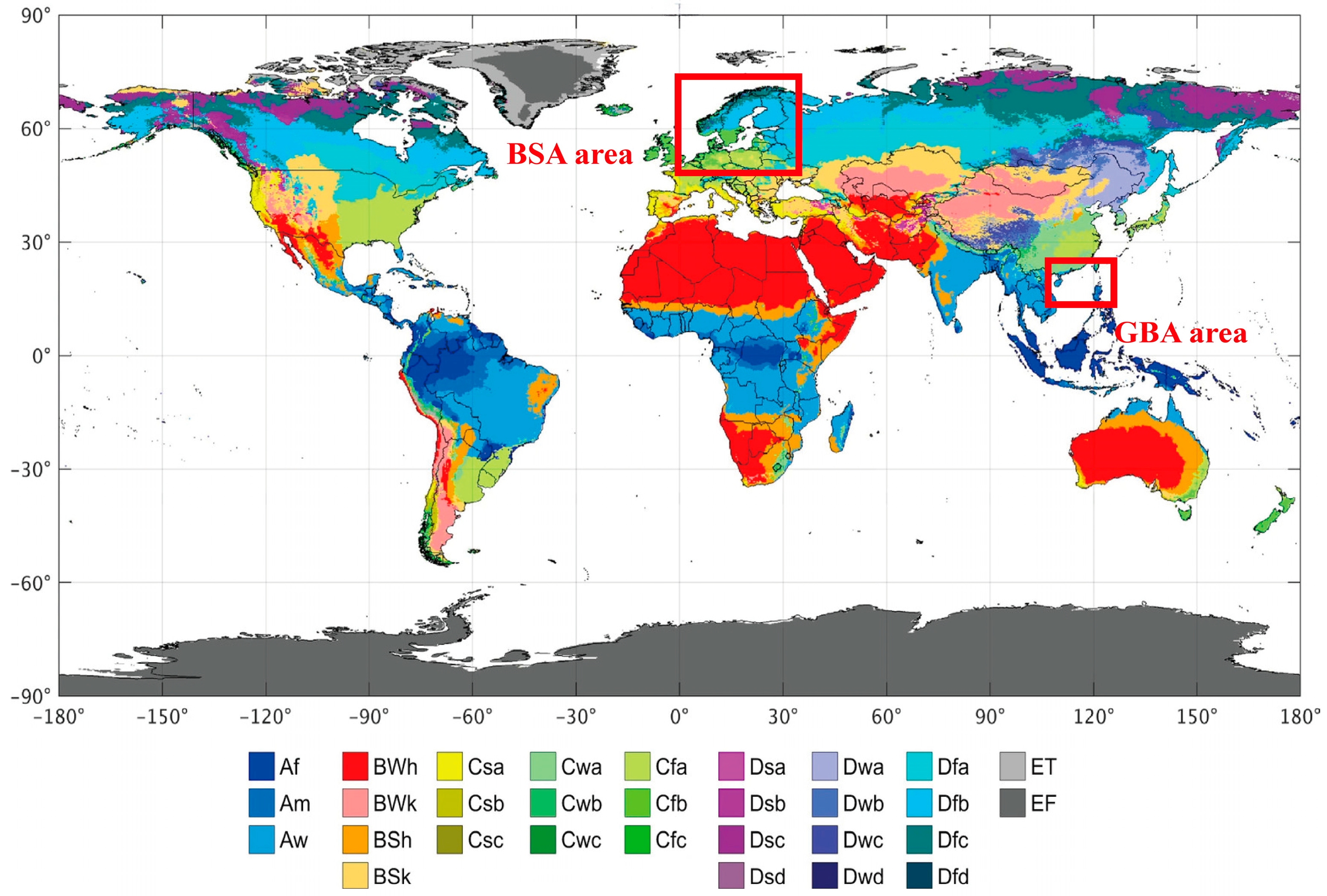
The BSA and GBA are representative coastal areas in both Europe and China, with different climate classifications and geographic positions [21] (Figure 1). Many scholars have carried out a large amount of work on climate changes in both areas. Thus, we can learn more about the facts and causes of climate change in both areas. In the GBA, researchers have mainly studied fact analysis of basic climatic elements and extreme events, multi-scale or trend extraction of mean temperature and precipitation, and brief attribution of climate change [22,23,24,25,26,27,28]. However, the results of different scholars are different in individual sites, which may be caused by the length of adopted data or the analysis method. For the studies in the BSA, scientists focus on the climate element changes of weather statistics such as temperature, precipitation, wind, humidity, cloud cover, and sea level in the whole BSA or a certain country. Meanwhile, the climate projection in the future and the attribution of climate change are also popular research issues in this region [29,30,31]. Moreover, some works have explored the results of multi-scale fluctuation of mean temperature and precipitation and some reasons for these climate changes in part of the BSA or adjacent areas [32,33,34]. However, taking the BSA as a whole representative region, the former multi-scale analyses are insufficient to extract the typical fluctuation scales. For regional climate, which is related to both large scales such as the global or hemisphere scale as well as local climate change, the influence factors are more complicated, and the characteristics of climate may be obvious regionally. In this work, we studied the similarities and differences of climate change between the two coastal areas. Thus, we selected the sites with the longest datasets as representative stations in both areas and adopted a unified analysis method to compare and analyze climate change, especially in multi-scale changes. Due to the limitation of the length of the data, temperature and precipitation were decomposed in this study because only these two elements have long-term records. In addition, climate data are usually nonlinear and non-stationary and exist as a mutual superposition of multi-scale signals. Thus, a self-adapting method, i.e., ensemble empirical mode decomposition (EEMD), was adopted in this study. This method is highly efficient and applicable to nonlinear and non-stationary signals. In Section 2, we introduce the data and method of this study. Section 3 gives the detailed results and analyses, and Section 4 and 5 contain discussion and conclusions.
2. Data and Method
2.1. Data
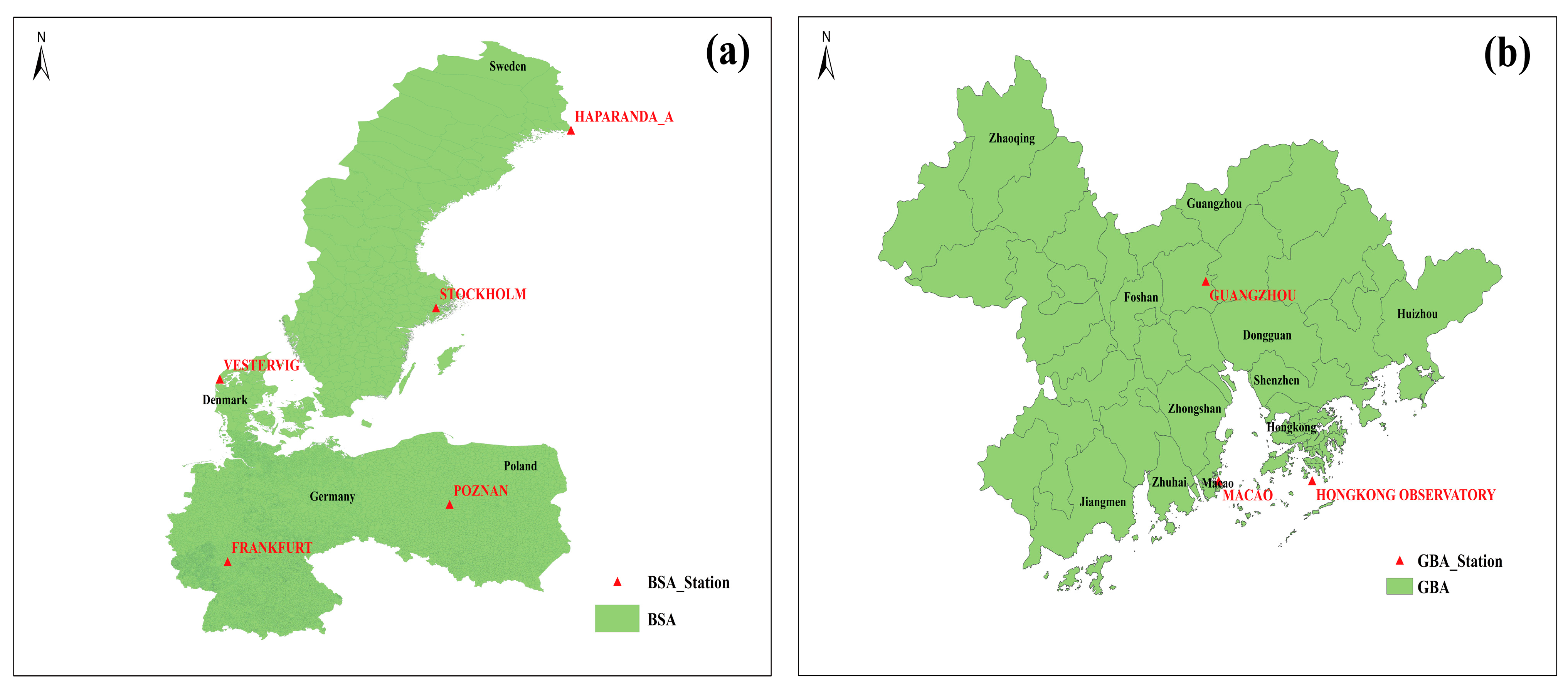
ECA&D (European Climate Assessment & Dataset) contains a series of daily observations at meteorological stations throughout Europe and the Mediterranean. In the BSA, we selected five stations (Stockholm, Haparanda_A, Vestervig, Poznan, and Frankfurt) from four countries (Sweden, Denmark, Poland, and Germany) as representative stations with the longest observed data and with few missing data. Three stations are located in the coastline area and two stations in the inland area (Figure 2a, Table 1). The daily datasets of precipitation and temperature used in this study were downloaded from https://www.ecad.eu/dailydata/index.php (accessedon 31 January 2020). For the daily series, we chose to use blended date, which means the gaps in daily series of stations were infilled with observations from nearby stations within 12.5 km distance and with a height difference of less than 25 m. For continuous missing data of some sites, especially for more than 8 days in a month, we established a regression equation between representative sites and several alternative stations to replace missing values, for which a Euclidean distance method was used to calculate the nearest stations as alternative stations. To make sure the replaced data were reliable, the sites with correlation coefficients of the recent five years of nearby missing data passing a 95% significance test were selected as alternative sites. The correlation coefficients (R2) of the regression equation were all above 0.68, which means the regression data can replace missing data well. Using daily data, which delete the scattered missing data after regression supplement, we calculated monthly mean temperature, monthly total precipitation, annual mean temperature, and annual total precipitation (Table 2). In the GBA, Guangzhou (in the inland area), Hong Kong, and Macao stations (in the coastline area) were chosen as representative stations (Figure 2b, Table 1). The monthly data of Guangzhou and Hong Kong came from Guangdong Climate Center and https://www.weather.gov.hk/tc/cis/climat.htm (accessed on 20 November 2022). The daily datasets of Macao were downloaded from https://frame.smg.gov.mo/centenary/index.htm (accessed on 20 November 2022). Using the same method for missing data in the BSA, we obtained monthly and annual data in the GBA (Table 3).
2.2. Method
Ensemble empirical mode decomposition (EEMD) is a noise-assisted and adaptive time-space data analysis method [35,36,37], which has been widely applied for extracting signals from nonlinear and nonstationary processes. The key algorithm of EEMD is empirical mode decomposition (EMD), which decomposes original data into a number of characteristic intrinsic mode function (IMF) components with different timescales and trends. To alleviate a major drawback of mode mixing in original EMD method, a white noise series of finite amplitude was added to original data to form new signals. By enough trials of EMD decomposition of new signals, the ensemble means of corresponding IMFs (Ci,i = 1,2,3…) are treated as the final results, which have physically meaningful signals in data [38,39]. As a powerful method, EEMD has been successfully applied to the research field of climate change, especially in multi-scale fluctuation analysis of climate elements such as temperature and precipitation [40,41,42,43]. For the climate mutation analysis of annual data, the Mann–Kendall (M-K) method was adopted in this study, and the results passed the 0.1 significance level.
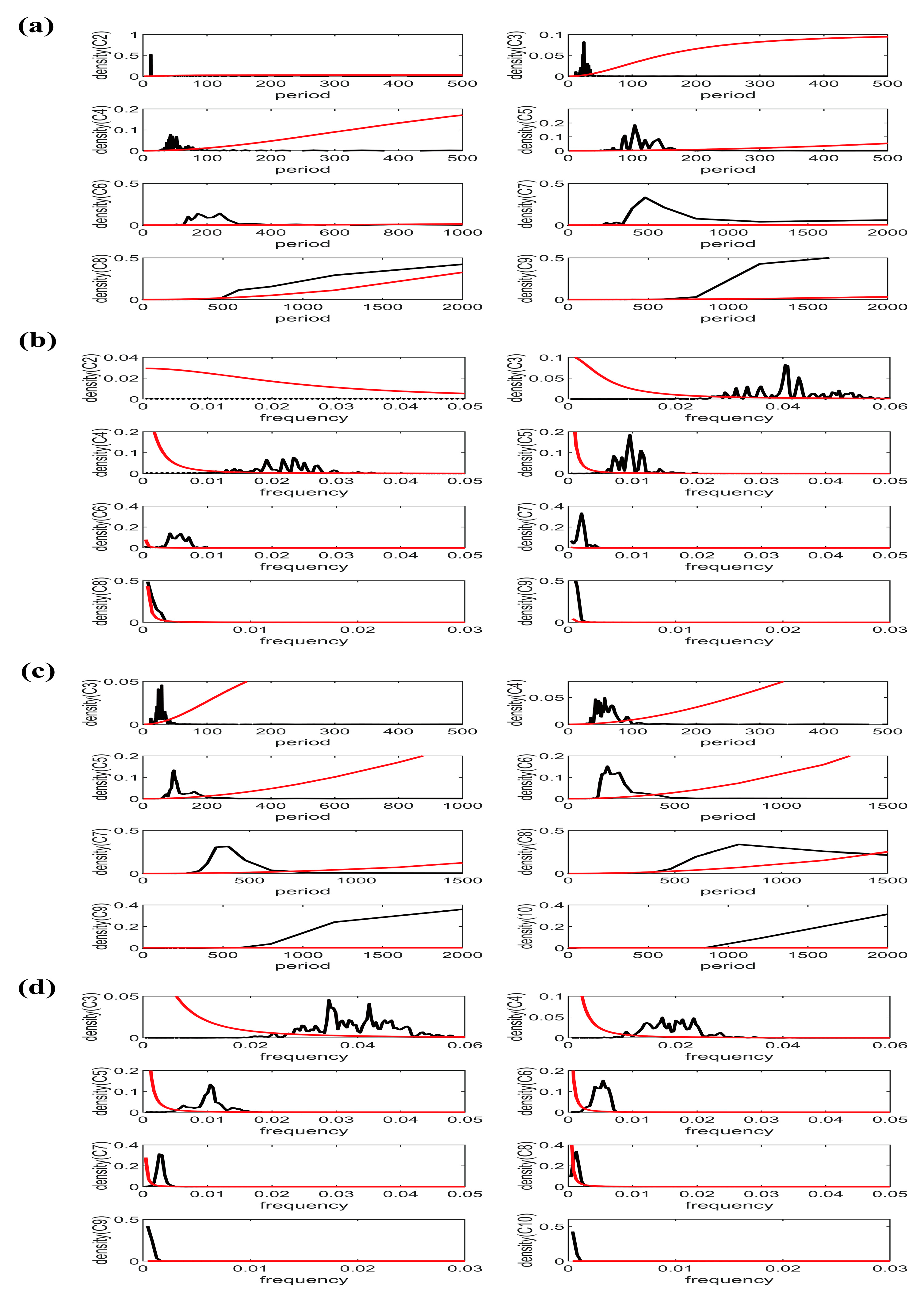
Based on the standardized monthly data processed by the Z-score method, we analyzed multi-scale fluctuations characterized with mean periods of temperature and precipitation in both the BSA and GBA. In EEMD decompositions, a standard deviation of 0.2 white noise series was added to original data, and the ensemble number of decomposition trials was 1000. In addition, we analyzed the power spectrum features of each IMF. The results show that in each IMF component, the fluctuation period or frequency may be varied throughout the whole timescale. Figure 3 shows examples of power spectrum density analysis of temperature IMFs at Hong Kong station (C2–C9) in the GBA and Stockholm station (C3–C10) in the BSA. The period or frequency with the maximum energy density of each IMF stands for the main period feature of corresponding timescale fluctuation, which passes the 95% significance test of red noise. Thus, in this study, we focused on multi-scale analysis of the mean period corresponding with mean instantaneous frequency and the main period corresponding with maximum density.
3. Results and Analyses
3.1. Climate Changes in Areas around Baltic Sea Area
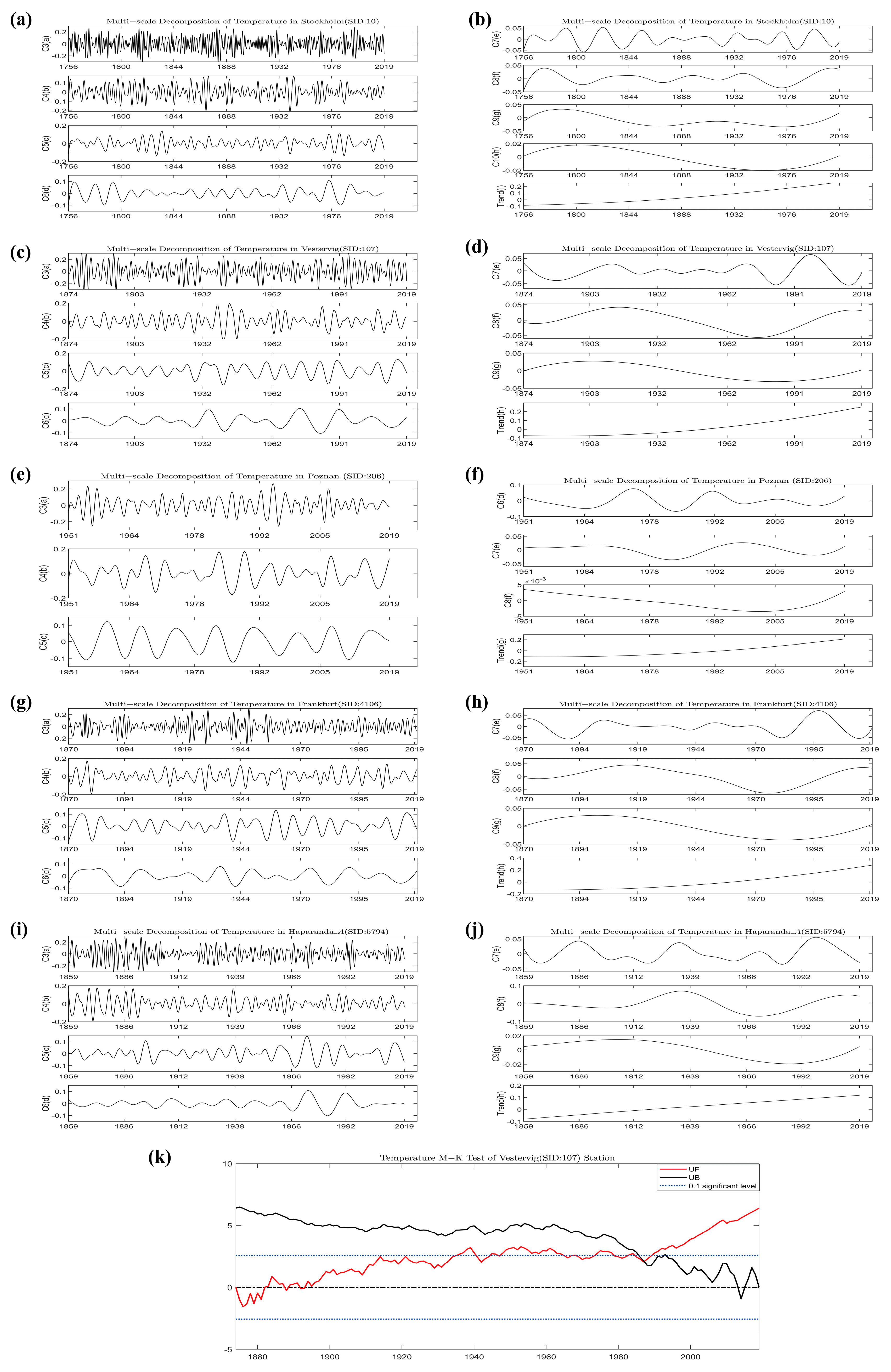
The temperature decomposition results of representative stations show that there are 8–10 IMFs and a residual component (trend) in the BSA. For all stations, IMF1 (C1) and IMF2 (C2) represent fluctuations under one year and annual cycle, which are not given in the table and figure because we focused on large-scale climate change with a more than one- year period. As shown in Figure 4, IMF3-5 (C3–C5) represent inter-annual scale, IMF6-8 (C6–C8) reveal inter-decadal variation, and IMF9-10 (C9–C10) indicate centennial scale fluctuation and the trend. The residual trend means a mean state of temperature change after the removal of multi-timescales. Table 4 lists all the results of fluctuation periods in each station. For the mean period, the timescales of inter-annual fluctuation are 2.0–4.3 and 7.4–8.5 a; the timescales of inter-decadal fluctuation are 13.2–18.0, 25.8–34.8, and 57.7–92.0 a; and the centennial scales are 143.6–184.7 and 264 a. For the main period of each IMF, the results may be slightly different from the mean period because of the different calculation methods. The main periods of the inter-annual scale are 1.8–6.1 and 7.7–8.3 a; the inter-decadal periods are 15.3–20.0, 28.5–50.0, and 66.6–99.0 a; and the centennial scale is 200–260 a. In order to calculate fluctuation features of different timescales, both mean period and main period were taken into consideration to obtain the summary results. The summary results should include as many fluctuation characteristics as possible. As shown in Table 4, we determined that the inter-annual scales in the BSA are 2–4 and 7–9 a, the inter-decadal scales are 13–20, 26–50, and 66–99 a; and the centennial scales are 143–185 and 200–264 a.
The residual components of representative stations in the BSA are shown in Figure 4b–j. It is shown that all the trends increased during the recorded time periods, but the increasing rates vary with stations or different time periods. Overall, the temperature change state of Haparanda_A station is a linear upward trend, and that of other stations shows a nonlinear increasing trend. To evaluate the mean rate of each site, we decomposed mean annual temperature by EEMD, and the residual trends show that the mean increasing rates of five stations (Stockholm, Vestervig, Poznan, Frankfurt, and Haparanda_A) are 0.10, 0.11, 0.40, 0.16, and 0.17 °C/10 a, respectively, which is very similar to the report on climate change in the Baltic Sea Area HELCOM thematic assessment in 2013. The mutation test results show that only Vestervig station changed abruptly in the year 1987, which passed the 0.1 significance level test. The other stations did not exhibit obvious temperature mutation points (Figure 4k).
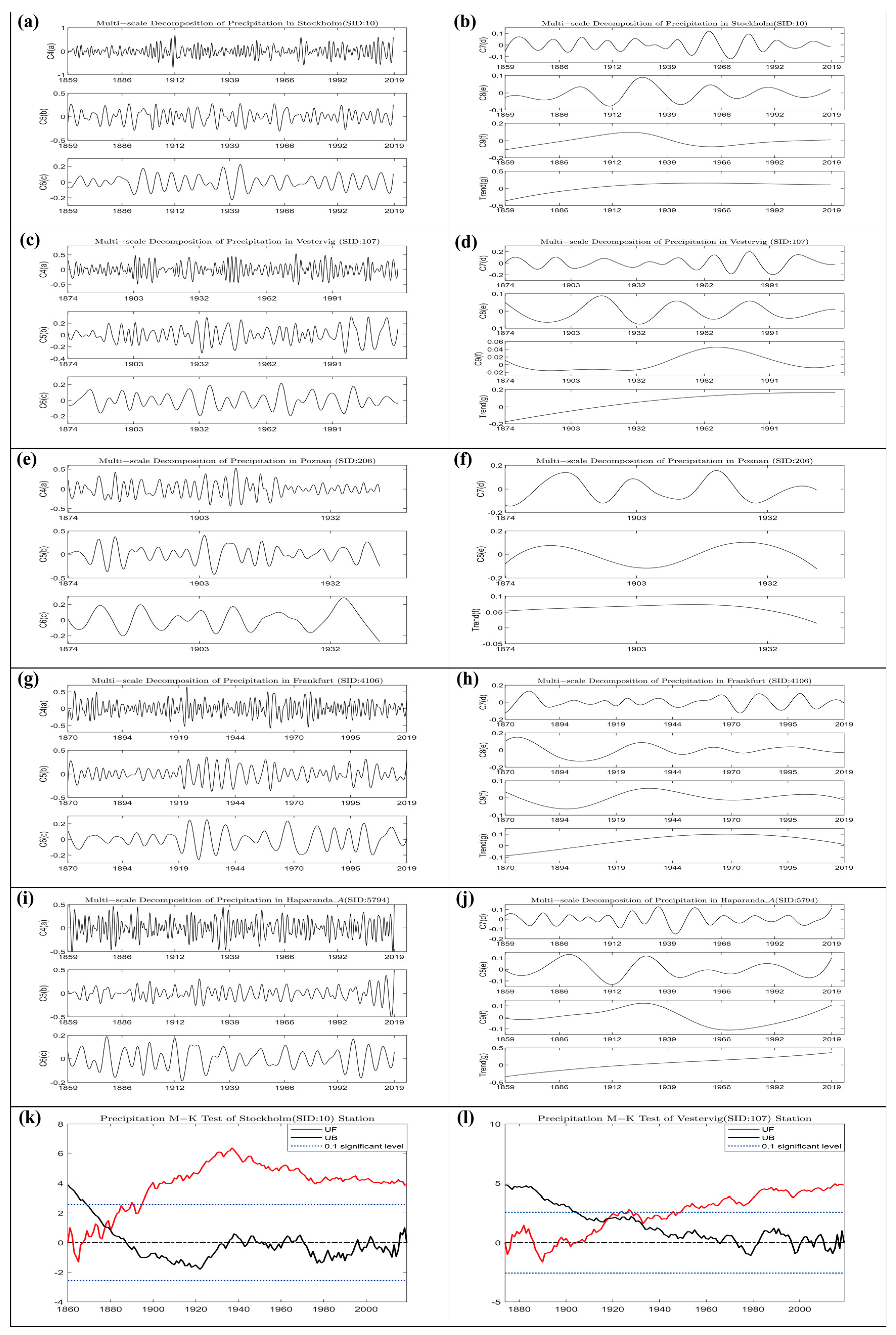
The results of precipitation decomposition revealed 8–9 IMFs (Figure 5). A slight difference with temperature decomposition is that C1–C3 represent timescales under one year and annual cycle. As shown in Table 5, C4–C6 represent inter-annual scales with mean period of 2.1–4.4 and 7.4–9.6 a, and the main periods are 2.0–3.3 and 4.2–8.0 a. C7–C8 reveal inter-decadal variations with mean periods of 14.4–18.6, 33.1–40.1, and 67.9–85.6 a, while the main periods are 11.0–20.0, 33–50, and 67–86 a. For the component of C9, fluctuation periods vary obviously over the whole timescale, especially in Vestervig and Frankfurt stations, which leads to the part of inter-decadal scale containing C9. Thus, we summarized this part of the period in the inter-decadal scale. The remaining scales were treated as centennial scales. As a result, the centennial scale of the mean period is 101.5–135.8 a, and that of the main period is 100.0–136.0 a. To summarize the final results comprehensively, the inter-annual scales of precipitation in the BSA are 2–4 and 7–9 a; the inter-decadal scales are 11–20, 33–50, and 67–86 a; and the centennial scale is 100–136 a.
As shown in Figure 5b–j, the trends of precipitation in the BSA are quite different from trends of temperature. The stations with a fluctuating trend are Stockholm, Poznan, and Frankfurt, which had a decreasing trend in recent decades. The stations with an upward trend are Vestervig and Haparanda_A stations. For the annual total precipitation, only Stockholm and Vestervig stations have mutation points in 1878 and 1918, respectively (Figure 5k,l).
3.2. Climate Changes in the Guangdong–Hong Kong–Macao Greater Bay
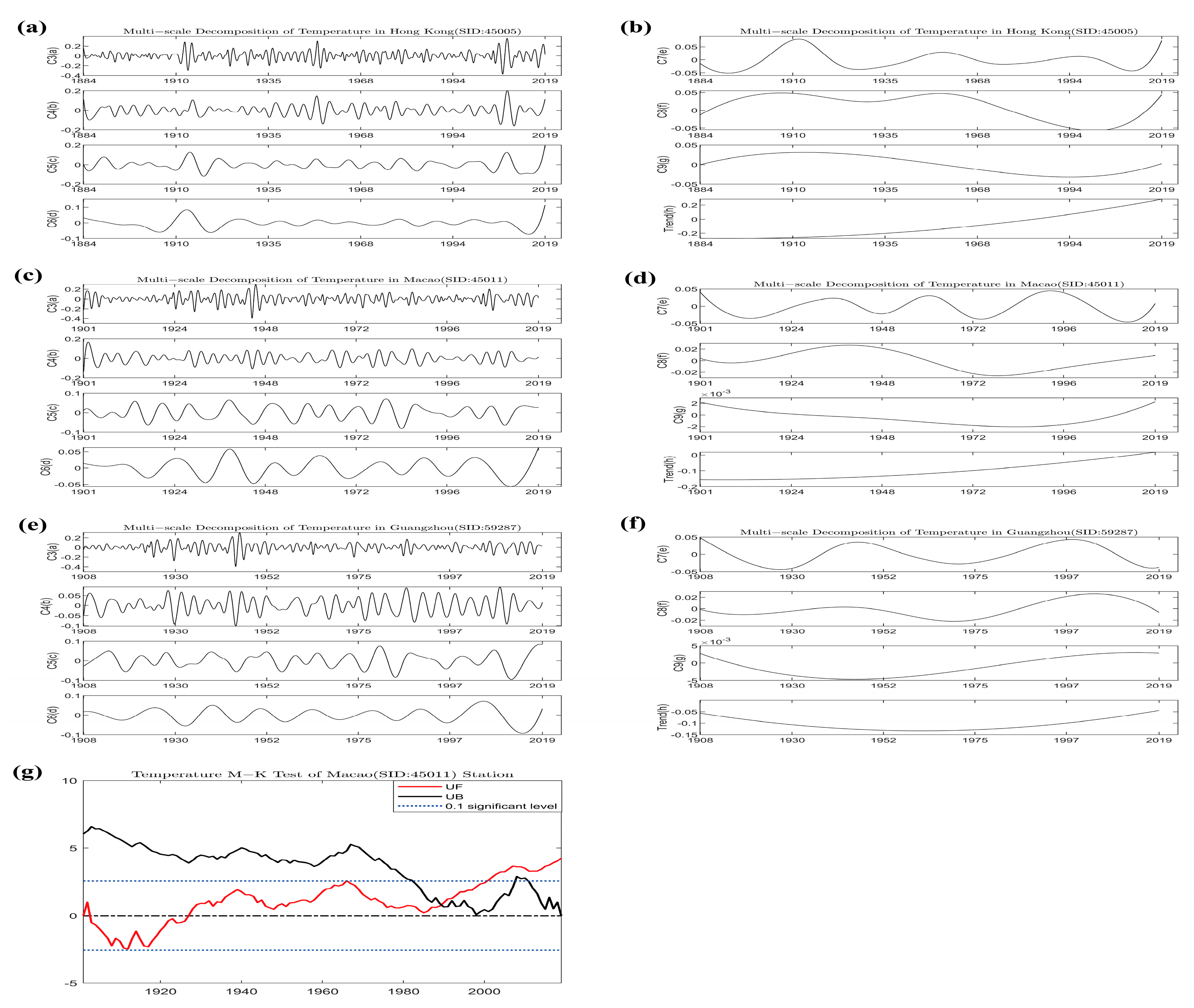
The temperature multi-scale changes are shown in Table 6 and Figure 6, with the elimination of less than one year and an annual cycle timescale. In the GBA, the mean period of inter-annual scales (C3–C5) are 1.8–3.6 and 8.3–8.7 a; inter-decadal scales (C6–C8) are 10.3–14.2, 30.0–45.0, and 55.2–92.4 a; and the centennial scale (C9) is 123.6–134.3 a. For the main period, the inter-annual timescales are 1.9–3.1 and 7.1–9.4 a; the inter-decadal scales are 13.3, 33.3–50.0, and 66.6–100 a; and the centennial scale is 100–199.8 a. The longest date length of the GBA is 136 a. Taking all factors (the length of data, the mean period, and main period) into consideration, we conclude that the inter-annual scales of temperature in the GBA are 2–4 and 7–9 a, which are the same as those of the BSA. The inter-decadal scales are 10–14, 30–50, and 55–99 a, which are quite different from those in the BSA. Perhaps due to the limitation of date length, the centennial scale in the GBA is 100–135 a, which is significantly different from that of the BSA. Figure 6b–h show the trends of three representative stations in the GBA. The Hong Kong and Macao stations change with a similar upward trend, but the increasing rate of Hong Kong is larger than that of Macao. Guangzhou station changes with a fluctuation trend, which means that before 1961, there was a downward trend, and then, temperature increased obviously, especially after 1980. The mutation test shows that only in Macao station did the mean annual temperature changed abruptly in the year 1991 (Figure 6g).
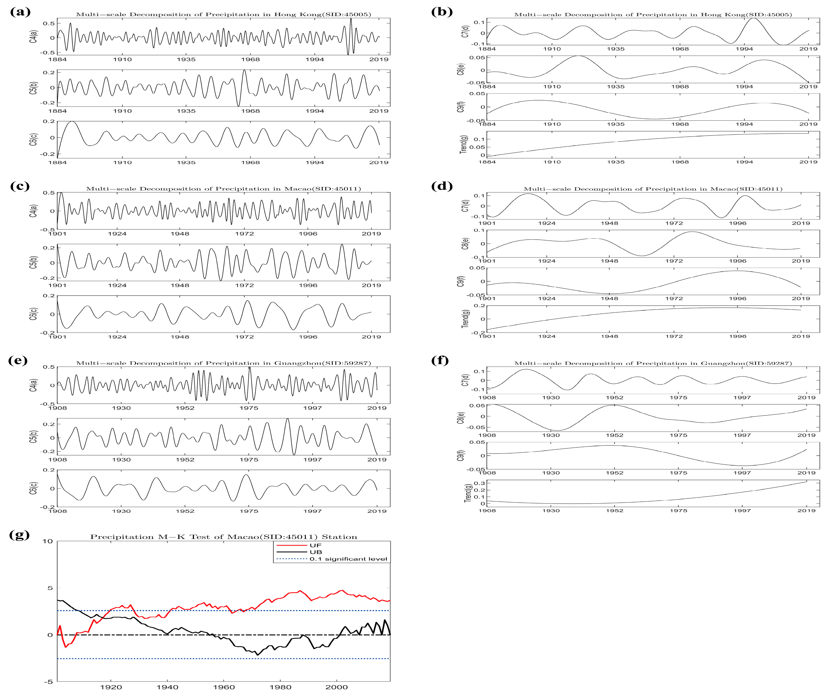
Table 7 provides multi-scales of fluctuation with timescales of more than one year of precipitation in the GBA. C4–C6 represent inter-annual scales with mean periods of 2.4–5.0 and 8.7–9.3 a and main periods of 2.5–3.4 and 6.0–6.7 a. C7–C8 show inter-decadal scales with mean periods of 20.2–25.6, 28.1–56.3, and 63.1–69.8 a and main periods of 10.5–11.8, 24.9–28.5, and 28.5–50 a. Adopting a similar data strategy as used in component of C9 in the BSA, we also extracted part of the inter-decadal period into a group of C7–C8. Thus, in the combined mean period and main period, the centennial scale is about 100 a, and the inter-decadal scales are 11–29 and 50–70 a. The inter-annual scales are 2–4 and 6–9 a, which are very similar to those of the BSA. As shown in Figure 7b–g, the residual trends of three stations fluctuated, but the variations are different. The trends of Hong Kong and Macao increased before 2006 and 1988, respectively, and after that decreased slowly. However, precipitation in Guangzhou station declined before 1945 and then rose dramatically. The mutation test also shows that only Macao station has a mutation point in 1917 (Figure 7g).
4. Discussion
In both the BSA and GBA, we extracted centennial, decadal, or multi-decadal and inter-annual scales and a general trend from each station. Although the fluctuation period of each site is slightly different, we still obtained a certain time range for each typical scale. It is well known that climate change may be influenced by internal and external forcing factors. Thus, possible forcing factors of a typical scale need to be discussed, and whether the factors are the same or not in two areas needs to be determined.
4.1. Forcing Factors of Inter-Annual Scale
For the inter-annual scale, both areas have very similar time ranges, mainly 2–4 and 7–9 or 6–9 a, and these results are very consistent with previous research [22,23,24,40]. Previous investigations have identified that oscillations of the inter-annual scale in the BSA are associated with large-scale circulation patterns such as the Arctic oscillation (AO) and the North Atlantic oscillation (NAO), which have a 2–8 a periodicity [33,34], while in the GBA, inter-annual oscillations have a relationship with ENSO with the same or one-year- ahead phase variation [22], which has a 2–7 a periodicity. Thus, the forcing factors of the inter-annual scale in both BSA and GBA are different and are, overall, caused by inter-annual oscillation of large-scale atmospheric circulation systems (AO, NAO) and interactions between atmosphere and the ocean (ENSO).
4.2. Forcing Factors of Decadal-to-Multidecadal or Centennial Scales
For the decadal-to-multidecadal timescales or centennial scale, the influence factors are more variable and complicated and always interact with each other, which usually influences a larger spatial range. Hence, when it comes to these scales, the uncertainty of climate change increases, and researchers may tend to investigate the causes of larger- scale climate change. In the BSA, a warming trend in the Baltic Sea area from 1958 to 2009 (about 51 a) is associated with changes in large-scale atmospheric circulation over the North Atlantic [19]. The large-scale circulation patterns (e.g., anticyclonic circulation, westerly winds) in the Baltic Sea region are influenced by the NAO, indicating that multi-decadal climate change in the Baltic Sea region is partly related to NAO [29]. In the North Atlantic–European region, decadal fluctuations of climate may be influenced by interactions between the atmosphere and the Atlantic Ocean [44]. Anthropogenic forcing can explain a large part of the observed changes from 1973 to 2002 (about 30 a) in temperature and precipitation over the Baltic Sea region [30,45], while in the GBA, there are few attribution studies on climate change. We can also investigate possible reasons from the large-scale attribution research such as studies in East China, the whole of China, and East Asia, which cover the GBA in space. Annual mean temperature with a quasi-60-year period in Macao consistently matches the variation of Atlantic multidecadal oscillation (AMO), and the quasi-30-year and quasi-60-year periods in summer and winter temperature in Macao have a statistically significant correlation with Pacific decadal oscillation (PDO) and AMO [19]. Urbanization, incoming solar radiation at the top of the atmosphere, and the modulated solar radiation reaching ground surface modulate multi-decadal variability in East China and the whole of China [46,47]. Tropical Indian Ocean sea-surface temperature (SST) and the Siberian atmospheric circulation systems accounted for at least 80% of total warming trends in East China during 1909–2010 [48]. For winter temperature, AMO (always with a period of 65–80 years), the East Asian winter monsoon (EAWM), PDO, and the Siberian high (SH) are linked to inter-decadal variation of winter temperature in East China and the whole of China [49,50,51,52]. For the East Asian summer rainfall (EASR), the decadal variation is modulated by Pacific sea-surface temperature anomalies (SSTAs) and inter-decadal oscillation patterns [53]. Thus, the forcing factors of the inter-decadal scale in the GBA seem more complex and are composed of atmospheric and ocean systems from different latitudes.
4.3. Forcing Factors of Multi-Decadal to Centennial Variation at Global or Hemispheric Scale
Furthermore, the multi-decadal to centennial variations of temperature have a global or hemispheric scale, while the average variation signal of precipitation at the global scale is not obvious because changes in precipitation in different regions cancel each other out. Natural forcing (e.g., changing orbital, solar, and volcanic forcing) increases the decadal–centennial timescale, and large spatial-scale temperature variability, especially pre-1850 and anthropogenic forcing (e.g., greenhouse gases, aerosol), has contributed significantly to 20th century temperature changes [54,55,56,57]. The variability in the Atlantic is a viable explanation for a portion of multi-decadal variation of Northern Hemisphere mean temperature [58]. Multi-decadal (65–70) oscillation of global mean temperature is the statistical result of 50–88-year oscillations for the North Atlantic Ocean and its bounding Northern Hemisphere continents and low-frequency variations of the thermohaline circulation [59,60]. In addition, decadal modulation factors of global mean temperature, such as AMO and PDO, also contribute significantly to the rates of decadal temperature cooling or warming [61,62]. Thus, the forcing factors of decadal–centennial scale for temperature are complicated and may have both general factors at a large scale and different regional factors, while the variation characteristics of precipitation are more regional because the influence factors vary in different regions.
5. Conclusions
Based on the comparison studies in both the BSA and GBA, we conclude that there are inter-annual-, inter-decadal-, and centennial-scale low-frequency fluctuations in both areas, but the low-frequency timescales differ. Climate trends and mutation results of temperature and precipitation vary in both areas.
For temperature, the inter-annual scales show the same results, with 2–4 and 7–9 a in both the GBA and BSA. The inter-decadal fluctuation has three main timescales in both the GBA and BSA, which are different and inconsistent. There are two main centennial scales in the BSA while only one in the GBA, which may be affected by the length of datasets. For precipitation, the timescales of the inter-annual fluctuation are consistent in both the GBA and BSA, similar to the temperature scales. The GBA has two main inter-decadal scales, while there are three in the BSA. For the centennial scale, there is only one main timescale in both the GBA and BSA.
The temperature trends of the GBA reveal that the coastal area has experienced an upward trend (Hong Kong and Macao stations), but in the inland area (Guangzhou), the trend has fluctuated, declining before 1961 and rising after 1961. This means the overall trend of the GBA increased after 1961 and accelerated obviously after 1980. Meanwhile, in the BSA, the temperature trends of all stations have experienced a rising trend with different growth rates. Most stations in the two regions have experienced a warming trend, which is consistent with the general situation of global warming. For the precipitation in the GBA, the trends of three stations show stronger local characteristics with different fluctuation types, while in the BSA, two stations (Haparanda_A and Vestervig) have experienced an upward trend throughout the whole time range, but the trends of three other stations have fluctuated, with a declining trend in recent decades. Overall, there are no unified trends for precipitation in both areas, which reveals that precipitation change is more complex and regional than temperature. The mutation tests show that there are no obvious regional temperature and precipitation mutations in both areas except at individual sites, such as Vestervig and Stockholm in the BSA and Macao in the GBA.
Author Contributions
Conceptualization, B.W. and J.Z. (Jinpeng Zhang); methodology, B.W., J.Z. (Jinpeng Zhang), and W.C.; software, J.Z. (Jing Zheng) and Y.X.; validation, J.Y.; formal analysis, B.W.; investigation, B.W. and J.Z. (Jinpeng Zhang); data curation, B.W. and J.Z. (Jing Zheng); writing—original draft preparation, B.W.; writing—review and editing, B.W. and J.Z. (Jinpeng Zhang); visualization, J.Z. (Jing Zheng); supervision, W.C. All authors have read and agreed to the published version of the manuscript.
Funding
The work was funded by Guangdong Basic and Applied Basic Research Foundation (No.:2021A1515011746); Guangdong Science and Technology Planning Key Program of Guangdong Meteorological Service (GRMC2019Z01); Guangdong Science and Technology Planning Program of Guangdong Meteorological Service (GRMC2018M20).
Data Availability Statement
The raw data supporting the conclusions of this article will be not available by the authors for the regulations from Guangdong Meteorological Service.
Acknowledgments
This research was carried out within bilateral international cooperative project implemented between the Guangzhou Marine Geological Survey (GMGS), China, and the University of Szczecin (USZ), Poland. This work is a contribution to the Deep-time Digital Earth (DDE) IUGS Big Science Program, with DDE-MS group. Thanks for the guidance and support from Professor Lisheng Tang and Hongyu Wu in Guangdong Climate Center.
Conflicts of Interest
The authors declare no conflict of interest.
References
- Kreft, S.; Eckstein, D.; Melchior, I. Global Climate Risk Index 2017: Who Suffers Most from Extreme Weather Events? Weather-Related Loss Events in 2015 and 1996 to 2015; Germanwatch e. V. Bonn.: Bonn, Germany, 2016; 32p, Available online: https://germanwatch.org/sites/germanwatch.org/files/publication/16411.pdf (accessed on 29 November 2016).
- McNamara, K.E.; Clissold, R.; Westoby, R. Women’s capabilities in disaster recovery and resilience must be acknowledged, utilized and supported. J. Gend. Stud. 2021, 30, 119–125. [Google Scholar] [CrossRef]
- Malik, A.A.; Stolove, J. In South Asian Slums, Women Face the Consequences of Climate Change, LEAD Pakistan, Islamabad. Available online: https://www.urban.org/urban-wire/south-asian-slums-women-face-consequencesclimate-change (accessed on 22 August 2017).
- Reguero, B.G.; Losada, I.J.; Méndez, F.J. A recent increase in global wave power as a consequence of oceanic warming. Nat. Commun. 2019, 10, 205. [Google Scholar] [CrossRef] [PubMed] [Green Version]
- Kulp, S.A.; Strauss, B.H. New elevation data triple estimates of global vulnerability to sea-level rise and coastal flooding. Nat. Commun. 2019, 10, 4844. [Google Scholar] [CrossRef] [PubMed] [Green Version]
- Mallick, B.; Ahmed, B.; Vogt, J. Living with the Risks of Cyclone Disasters in the South-Western Coastal Region of Bangladesh. Environments 2017, 4, 13. [Google Scholar] [CrossRef]
- Pörtner, H.O.; Alegría, A.; Möller, V.; Poloczanska, E.S.; Mintenbeck, K.; Götze, S. Annex I: Global to Regional Atlas. In Climate Change 2022: Impacts, Adaptation and Vulnerability; Contribution of Working Group II to the Sixth Assessment Report of the Intergovernmental Panel on Climate Change; Cambridge University Press: Cambridge, UK; New York, NY, USA, 2022; pp. 2811–2896. [Google Scholar] [CrossRef]
- Pörtner, H.O.; Roberts, D.C.; Poloczanska, E.S.; Mintenbeck, K.; Tignor, M.; Alegría, A.; Craig, M.; Langsdorf, S.; Löschke, S.; Möller, V.; et al. Summary for Policymakers. In Climate Change 2022: Impacts, Adaptation and Vulnerability; Contribution of Working Group II to the Sixth Assessment Report of the Intergovernmental Panel on Climate Change; Cambridge University Press: Cambridge, UK; New York, NY, USA, 2022; pp. 3–33. [Google Scholar] [CrossRef]
- Zhou, C.S.; Luo, L.J.; Shi, C.Y.; Wang, J.H. Spatio-temporal Evolutionary Characteristics of the Economic Development in the Guangdong-Hong Kong-Macao Greater Bay Area and Its Influencing Factors. Trop. Geogr. 2017, 37, 802–813. [Google Scholar]
- Liu, Y.X. Research and Implications of Bay Zone Economy Home and Abroad. Urban Insight 2014, 3, 155–162. [Google Scholar]
- FEMA. Coastal AE Zone and VE Zone Demographics Study and Primary Frontal Dune Study to Support the NFIP; Federal Emergency Management Agency Technical Report; Federal Emergency Management Agency: Washington, DC, USA, 2008; 98p. [Google Scholar]
- Moser, S.C.; Davidson, M.A.; Kirshen, P.; Mulvaney, P.; Murley, J.F.; Neumann, J.E.; Petes, L.; Reed, D. Chapter 25: Coastal Zone Development and Ecosystems. In Climate Change Impacts in the United States: The Third National Climate Assessment; Melillo, J.M., Richmond, T.C., Yohe, G.W., Eds.; U.S. Global Change Research Program: Washington, DC, USA, 2014; pp. 579–618. [Google Scholar]
- Walsh, J.; Wuebbles, D.; Hayhoe, K.; Kossin, J.; Kunkel, K.; Stephens, G.; Thorne, P.; Vose, R.; Wehner, M.; Willis, J.; et al. Chapter 2: Our Changing Climate. In Climate Change Impacts in the United States: The Third National Climate Assessment; Melillo, J.M., Richmond, T.C., Yohe, G.W., Eds.; U.S. Global Change Research Program: Washington, DC, USA, 2014; pp. 19–67. [Google Scholar]
- Rhein, M.; Rintoul, S.R.; Aoki, S.; Campos, E.; Chambers, D.; Feely, R.A.; Gulev, S.; Johnson, G.C.; Josey, S.A.; Kostianoy, A.; et al. Observations: Ocean. In Climate Change 2013: The Physical Science Basis; Contribution of Working Group I to the Fifth Assessment Report of the Intergovernmental Panel on Climate Change; Stocker, T.F., Qin, D., Plattner, G.K., Tignor, M., Allen, S.K., Boschung, J., Nauels, A., Xia, Y., Bex, V., Midgley, P.M., Eds.; Cambridge University Press: Cambridge, UK; New York, NY, USA, 2013; pp. 255–316. [Google Scholar] [CrossRef] [Green Version]
- Wong, P.P.; Losada, I.J.; Gattuso, J.; Hinkel, J.; Khattabi, A.; McInnes, K.; Saito, Y.; Sallenger, A. Coastal systems and low-lying areas. In Climate Change 2014: Impacts, Adaptation, and Vulnerability; Contribution of Working Group II to the Fifth Assessment Report of the Intergovernmental Panel on Climate Change; Field, C.B., Barros, V.R., Dokken, D.J., Mach, K.J., Mastrandrea, M.D., Bilir, T.E., Chatterjee, M., Ebi, K.L., Estrada, Y.O., Genova, R.C., et al., Eds.; Cambridge University Press: Cambridge, UK; New York, NY, USA, 2014; pp. 361–409. [Google Scholar]
- Burkett, V.R.; Hyman, R.C.; Hagelman, R.; Hartley, S.B.; Sheppard, M.; Doyle, T.W.; Beagan, D.M.; Meyers, A.; Hunt, D.T.; Maynard, M.K.; et al. Why Study the Gulf Coast? In Impacts of Climate Change and Variability on Transportation Systems and Infrastructure: Gulf Coast Study, Phase I. Department of Transportation; U.S. Climate Change Science Program: Washington, DC, USA, 2008. [Google Scholar]
- Karl, T.R.; Melillo, J.M.; Peterson, T.C. Global Climate Change Impacts in the United States, United States Global Change Research Program; Cambridge University Press: Cambridge, UK, 2009; pp. 145–149. [Google Scholar]
- Qian, G.M.; Lv, Y.P.; Du, Y.D.; Chen, X.G.; Wang, C.L.; Tang, H.Y. Guangdong Province Climate Business Technical Manual; China Meteorological Press: Beijing, China, 2008. (In Chinese) [Google Scholar]
- Lehmann, A.; Getzlaff, K.; Harlaß, J. Detailed assessment of climate variability in the Baltic Sea area for the period 1958 to 2009. Clim. Res. 2011, 46, 185–196. [Google Scholar] [CrossRef]
- HELCOM. Climate change in the Baltic Sea Area: HELCOM thematic assessment in 2013. Balt. Sea Environ. Proc. 2013, 137, 3–24. [Google Scholar]
- Beck, H.E.; Zimmermann, N.E.; McVicar, T.R.; Vergopolan, N.; Berg, A.; Wood, E.F. Present and future Köppen-Geiger climate classification maps at 1-km resolution. Sci. Data 2018, 5, 180214. [Google Scholar] [CrossRef] [Green Version]
- Kong, F. Characteristics of temperature time series in Hong Kong and Macao in the past 100 years and their correlation with ENSO. Water Resour. Hydropower Eng. 2020, 51, 45–53. (In Chinese) [Google Scholar]
- Fong, S.K.; Wu, C.S.; Wang, T.; He, X.J.; Wang, A.Y.; Liu, J.; Liang, B.Q.; Leong, K.C. Multiple time scales analysis of climate variation in Macao during the last 100 years. J. Trop. Meteorol. 2010, 26, 452–462. (In Chinese) [Google Scholar]
- Ji, Z.P.; Gu, D.J.; Xie, J.G. Multiple time scales analysis of climate variation in Guangzhou during the last 100 years. J. Trop. Meteorol. 1999, 15, 48–55. (In Chinese) [Google Scholar]
- Zhou, W.; Jian, Y.G.; Chen, C.M.; Liang, J.J. The impact of El Nino and Asian monsoons on rainfall of Hong Kong and Macao. Trop. Geogr. 2001, 21, 36–40. (In Chinese) [Google Scholar]
- Wu, J.; Xu, Y.; Shi, Y. Urbanization effects on local climate change in South China. Clim. Environ. Res. 2015, 6, 654–661. (In Chinese) [Google Scholar]
- Han, C.F. Asian Monsoon Climate Change and Effects of Different External Forcings during Historical Period; Nanjing Normal University: Nanjing, China, 2017. (In Chinese) [Google Scholar]
- Du, Y.D.; Zhang, Y.; Lu, H.; Duan, H.L.; Luo, X.L.; Liu, C.H.J.; Li, Y.L.; Zhang, Y.J.; Huang, C.R.; Hu, F.; et al. Assessment Report of Climate Change in South China: 2020; China Meteorological Press: Beijing, China, 2021. (In Chinese) [Google Scholar]
- Omstedt, A.; Pettersen, C.; Rodhe, J.; Winsor, P. Baltic Sea Climate: 200Yr of Data on Air Temperature, Sea Level Variation, Ice Cover, and Atmospheric Circulation. Clim. Res. 2004, 25, 205–216. [Google Scholar] [CrossRef] [Green Version]
- Bhend, J.; Storch, V. Consistency of observed winter precipitation trends in northern Europe with regional climate change projections. Clim. Dyn. 2008, 31, 17–28. [Google Scholar] [CrossRef] [Green Version]
- Stips, A.; Lilover, M. Yet Another Assessment of Climate Change in the Baltic Sea Area: Breakpoints in Climate Time Serie. In Proceedings of the 2010 IEEE/OES Baltic International Symposium (BALTIC), Riga, Latvia, 24–27 August 2010; pp. 1–9. [Google Scholar] [CrossRef]
- Eriksson, C.; Omstedt, A.; James, E.O.; Donald, B.P.; Harold, O.M. Characterizing the European SubArctic Winter Climate since 1500 Using Ice, Temperature, and Atmospheric Circulation Time Series. J. Clim. 2007, 20, 5316–5334. [Google Scholar] [CrossRef] [Green Version]
- Appenzeller, C.; Stocker, T.F.; Anklin, M. North Atlantic Oscillation dynamics recorded in Greenland ice cores. Science 1998, 282, 446–449. [Google Scholar] [CrossRef]
- Chen, D.L.; Hellström, C. The influence of the North Atlantic Oscillation on the regional temperature variability in Sweden: Spatial and temporal variations. Tellus 1999, 51, 505–516. [Google Scholar] [CrossRef] [Green Version]
- Huang, N.E.; Shen, Z.; Long, S.R.; Manli, C.W.; Hsing, H.S.; Zheng, Q.; Yen, N.C.; Tung, C.C.; Liu, H.H. The empirical mode decomposition and the Hilbert spectrum for nonlinear and nonstationary time series analysis. Proc. R. Soc. A 1998, 454, 903–995. [Google Scholar] [CrossRef]
- Flandring, P.; Rilling, G.; Goncalves, P. Empirical mode decomposition as a filterbank. IEEE Signal. Proc. Lett. 2004, 11, 112–114. [Google Scholar] [CrossRef] [Green Version]
- Wu, Z.H.; Huang, N.E.; Long, S.R.; Peng, C.K. On the trend detrending and the variability of nonlinear and nonstationary time series. Proc. Natl. Acad. Sci. USA 2007, 104, 14889–14894. [Google Scholar] [CrossRef] [PubMed] [Green Version]
- Wu, Z.H.; Huang, N.E. A study of the characteristics of white noise using the empirical mode decomposition method. Proc. R. Soc. A 2004, 460, 1597–1611. [Google Scholar] [CrossRef]
- Wu, Z.H.; Huang, N.E. Ensemble empirical mode decomposition: A noise-assisted data analysis method. Adv. Adapt. Data Anal. 2009, 1, 1–41. [Google Scholar] [CrossRef]
- Wang, B.; Li, X.D. Multi-Scale fluctuation of European temperature revealed by EEMD analysis. Acta Sci. Nat. Univ. Pekin. 2011, 47, 627–635. (In Chinese) [Google Scholar]
- Wang, B.; Hu, Y.M.; Du, Y.D.; Zhai, Z.H.; Wu, X.X. Study on the difference between wavelet analysis and EEMD in multi-scale decomposition of the temperature and precipitation of Guangzhou. J. Trop. Meteorol. 2014, 30, 769–776. (In Chinese) [Google Scholar]
- Sun, X.; Lin, Z.S.; Cheng, X.X.; Jiang, C.Y. Regional features of the temperature trend in China based on the empirical mode decomposition. J. Geogr. Sci. 2008, 18, 166–176. [Google Scholar] [CrossRef]
- Li, H.Q.; Fu, Z.T. Sunshine duration’s trend behavior based on EEMD over China in 1956–2005. Acta Sci. Nat. Univ. Pekin. 2012, 48, 393–398. (In Chinese) [Google Scholar]
- Venzke, S.; Allen, M.R.; Sutton, R.T.; Rowell, D.P. The Atmospheric Response over the North Atlantic to Decadal Changes in Sea Surface Temperature. J. Clim. 1999, 12, 2562–2584. [Google Scholar] [CrossRef]
- Bhend, J.; Storch, H. Is greenhouse gas warming a plausible explanation for the observed warming in the Baltic Sea catchment area? Boreal Environ. Res. 2009, 14, 81–88. [Google Scholar]
- Qian, C. Disentangling the urbanization effect, multi-decadal variability, and secular trend in temperature in eastern China during 1909–2010. Environ. Sci. 2016, 2, 177–182. [Google Scholar] [CrossRef] [Green Version]
- Soon, W.; Dutta, K.; Legates, D.R.; Velasco, V.; Zhang, W.J. Variation in surface air temperature of China during the 20th century. J. Atmos. Sol.-Terr. Phys. 2011, 73, 2331–2344. [Google Scholar] [CrossRef]
- Zhao, P.; Jones, P.; Cao, L.J.; Yan, Z.W.; Zha, S.Y.; Zhu, Y.N.; Yu, Y.; Tang, G.L. Trend of surface air temperature in eastern China and associated large-scale climate variability over the last 100 years. J. Clim. 2014, 27, 4693–4703. [Google Scholar] [CrossRef]
- Li, S.L.; Bates, G.T. Influence of the Atlantic Multidecadal Oscillation on the Winter Climate of East China. Adv. Atmos. Sci. 2007, 24, 126–135. [Google Scholar] [CrossRef]
- Wang, J.L.; Yang, B.; Ljungqvist, F.C.; Zhao, Y. The relationship between the Atlantic multidecadal oscillation and temperature variability in China during the last millennium. J. Quat. Sci. 2013, 28, 653–658. [Google Scholar] [CrossRef]
- Yun, J.H.; Ha, K.J.; Jo, Y.H. Interdecadal changes in winter surface air temperature over East Asia and their possible causes. Clim. Dyn. 2018, 51, 1375–1390. [Google Scholar] [CrossRef]
- Xu, Y.F.; Li, T.; Shen, S.H.; Hu, Z.H. Assessment of CMIP5 Models Based on the Interdecadal Relationship between the PDO and Winter Temperature in China. Atmosphere 2019, 10, 597. [Google Scholar] [CrossRef] [Green Version]
- Kim, S.Y.; Ha, K.J. Interannual and decadal covariabilities in East Asian and Western North Pacific summer rainfall for 1979–2016. Clim. Dyn. 2021, 56, 1017–1033. [Google Scholar] [CrossRef]
- Tett, S.F.B.; Betts, R.A.; Crowley, T.J.; Gregory, J. The impact of natural and anthropogenic forcings on climate and hydrology since 1550. Clim. Dyn. 2007, 28, 3–34. [Google Scholar] [CrossRef]
- Crowley, T.J. Causes of climate change over the past 1000 years. Science 2000, 289, 270–277. [Google Scholar] [CrossRef] [Green Version]
- Hegerl, G.C.; Hasselmann, K.; Cubasch, U.; Mitchell, J.F.B.; Roeckner, E.; Voss, R.; Waszkewitz, J. Multi-fingerprint detection and attribution analysis of greenhouse gas, greenhouse gas-plus-aerosol and solar forced climate change. J. Clim. Dyn. 1997, 13, 613–634. [Google Scholar] [CrossRef] [Green Version]
- Manabe, S.; Stouffer, R.J. Climate variability of a coupled ocean-atmosphere-land surface model: Implication for the detection of global warming. Bull. Am. Meteorol. Soc. 1997, 78, 1177–1185. [Google Scholar]
- Zhang, R.; Delworth, T.L.; Held, I.M. Can the Atlantic Ocean drive the observed multidecadal variability in Northern Hemisphere mean temperature? Geophys. Res. Lett. 2007, 34, 1–6. [Google Scholar] [CrossRef] [Green Version]
- Schlesinger, M.; Ramankutty, N. An Oscillation in the global climate system of period 65–70 years. Nature 1994, 367, 723–726. [Google Scholar] [CrossRef]
- Wu, Z.H.; Huang, N.E.; Wallace, J.M.; Smoliak, B.V.; Chen, X.Y. On the time-varying trend in global-mean surface temperature. Clim. Dyn. 2011, 37, 759–773. [Google Scholar] [CrossRef] [Green Version]
- Delsole, T.; Tippett, M.K.; Shukla, J. A Significant Component of Unforced Multidecadal Variability in the Recent Acceleration of Global Warming. J. Clim. 2011, 24, 909–926. [Google Scholar] [CrossRef] [Green Version]
- Dai, A.G.; Fyfe, J.C.; Xie, S.P.; Dai, X.G. Decadal modulation of global surface temperature by internal climate variability. Nat. Clim. Chang. 2015, 5, 555–559. [Google Scholar] [CrossRef]
Figure 1.
New and improved present-day Köppen–Geiger classification map (1980–2016) and areas we selected (GBA and BSA) (Beck 2020).
Figure 1.
New and improved present-day Köppen–Geiger classification map (1980–2016) and areas we selected (GBA and BSA) (Beck 2020).

Figure 2.
Representative stations in BSA area (a) and in GBA area (b).

Figure 3.
Power spectrum analysis of IMFs at Hong Kong in GBA (period-density (a), frequency-density (b)) and Stockholm in BSA (period-density (c), frequency-density (d)).
Figure 3.
Power spectrum analysis of IMFs at Hong Kong in GBA (period-density (a), frequency-density (b)) and Stockholm in BSA (period-density (c), frequency-density (d)).

Figure 4.
IMFs and trends of mean monthly temperature in Stockholm station (a,b), Vestervig station (c,d), Poznan station (e,f), Frankfurt station (g,h), and Haparanda_A station (i,j); temperature M-K test of Vestervig station (k).
Figure 4.
IMFs and trends of mean monthly temperature in Stockholm station (a,b), Vestervig station (c,d), Poznan station (e,f), Frankfurt station (g,h), and Haparanda_A station (i,j); temperature M-K test of Vestervig station (k).

Figure 5.
IMFs and trends of mean monthly precipitation in Stockholm station (a,b), Vestervig station (c,d), Poznan station (e,f), Frankfurt station (g,h), and Haparanda_A station (i,j); precipitation M-K test of Stockholm station (k) and Vestervig station (l).
Figure 5.
IMFs and trends of mean monthly precipitation in Stockholm station (a,b), Vestervig station (c,d), Poznan station (e,f), Frankfurt station (g,h), and Haparanda_A station (i,j); precipitation M-K test of Stockholm station (k) and Vestervig station (l).

Figure 6.
IMFs and trend of mean monthly temperature in Hong Kong (a,b), Macao (c,d), and Guangzhou station (e,f) and temperature M-K test of Macao station (g).
Figure 6.
IMFs and trend of mean monthly temperature in Hong Kong (a,b), Macao (c,d), and Guangzhou station (e,f) and temperature M-K test of Macao station (g).

Figure 7.
IMFs and trend of monthly total precipitation in Hong Kong (a,b), Macao (c,d), and Guangzhou station (e,f) and precipitation M-K test of Macao station (g).
Figure 7.
IMFs and trend of monthly total precipitation in Hong Kong (a,b), Macao (c,d), and Guangzhou station (e,f) and precipitation M-K test of Macao station (g).


Table 1.
The information of the representative stations in both areas around Baltic Sea area and the Guangdong–Hong Kong–Macao Greater Bay area.
Table 1.
The information of the representative stations in both areas around Baltic Sea area and the Guangdong–Hong Kong–Macao Greater Bay area.
| Areas around Baltic Sea Area (BSA) | |||||
|---|---|---|---|---|---|
| Station Name | Station ID | Country Code (CN) | Latitude (°N) | Longitude (°E) | Height (m) |
| Stockholm | 10 | Sweden (SE) | 59.35 | 18.05 | 44.00 |
| Vestervig | 107 | Denmark (DK) | 56.77 | 8.32 | 18.00 |
| Poznan | 206 | Poland (PL) | 52.20 | 18.66 | 115.00 |
| Frankfurt | 4106 | Germany (DE) | 50.13 | 8.67 | 124.00 |
| Haparanda_A | 5794 | Sweden (SE) | 65.82 | 24.12 | 16.00 |
| The Guangdong–Hong Kong–Macao Greater Bay (GBA) | |||||
| Station Name | Station ID | Country code (CN) | Latitude (°N) | Longitude (°E) | Height (m) |
| Guangzhou | 59,287 | China (CN) | 23.22 | 113.48 | 70.70 |
| Hong Kong | 45,005 | Hongkong (HK) | 22.29 | 114.17 | 32.00 |
| Macao | 45,011 | Macao (MO) | 22.20 | 113.53 | 110.00 |
Note: Country code (ISO3116 country codes).
Table 2.
Data processing information of the representative stations in areas around the Baltic Sea area.
Table 2.
Data processing information of the representative stations in areas around the Baltic Sea area.
| Temperature | |||||
|---|---|---|---|---|---|
| Station ID | 10 | 107 | 206 | 4106 | 5794 |
| Length of original data (daily) | 96,424 | 53,113 | 25,202 | 54,786 | 58,592 |
| Length of correction data (daily) | 96,424 | 53,076 | 25,202 | 54,786 | 58,559 |
| Length of correction data (monthly) | 1756.01– 2019.12 | 1874.08– 2019.12 | 1951.01– 2019.12 | 1870.01– 2019.12 | 1859.08– 2019.12 |
| Length of correction data (year) | 1756–2019 | 1875–2019 | 1951–2019 | 1870–2019 | 1860–2019 |
| Precipitation | |||||
| Station ID | 10 | 107 | 206 | 4106 | 5794 |
| Length of original data (daily) | 58,804 | 53,325 | 25,202 | 54,786 | 58,608 |
| Length of correction data (daily) | 58,804 | 53,104 | 25,197 | 54,786 | 58,585 |
| Length of correction data (monthly) | 1859.01– 2019.12 | 1874.01– 2019.12 | 1951.01– 2019.12 | 1870.01– 2019.12 | 1859.07– 2019.12 |
| Length of correction data (year) | 1859–2019 | 1874–2019 | 1951–2019 | 1870–2019 | 1860–2019 |
Table 3.
Data processing information of the representative stations in The Guangdong–Hong Kong–Macao Greater Bay area.
Table 3.
Data processing information of the representative stations in The Guangdong–Hong Kong–Macao Greater Bay area.
| Temperature | ||||
|---|---|---|---|---|
| Station ID | 45,005 | 59,287 | Station ID | 45,011 |
| Length of original data (monthly) | 1884.01– 2019.12 | 1908.01– 2019.12 | Length of original data (daily) | 1901.01– 2019.12 |
| Length of correction data (monthly) | 1884.04– 2019.12 | 1908.01– 2019.12 | Length of correction data (monthly) | 1901.01– 2019.12 |
| Length of correction data (year) | 1885–2019 | 1908–2019 | Length of correction data (year) | 1901–2019 |
| Precipitation | ||||
| Station ID | 45,005 | 59,287 | Station ID | 45011 |
| Length of original data (monthly) | 1884.01– 2019.12 | 1908.01– 2019.12 | Length of original data (daily) | 1901.01– 2019.12 |
| Length of correction data (monthly) | 1884.01– 2019.12 | 1908.01– 2019.12 | Length of correction data (monthly) | 1901.01– 2019.12 |
| Length of correction data (year) | 1884–2019 | 1908–2019 | Length of correction data (year) | 1901–2019 |
Table 4.
Multi-scale periodic analysis of temperature in areas around the Baltic Sea area (BSA).
| Mean Periods of IMFs in BSA Area (Unit: a) | ||||||||
|---|---|---|---|---|---|---|---|---|
| IMFs | C3 | C4 | C5 | C6 | C7 | C8 | C9 | C10 |
| 10 | 2.0 | 4.0 | 7.6 | 14.0 | 28.0 | 57.7 | 184.7 | 264 |
| 107 | 2.1 | 4.2 | 7.9 | 14.5 | 25.8 | 92 | 143.4 | |
| 206 | 2.1 | 4.1 | 8.5 | 18.0 | 33.7 | 71.4 | ||
| 4106 | 1.9 | 4.3 | 7.5 | 15.6 | 29.4 | 77.6 | 149.8 | |
| 5794 | 2.0 | 3.9 | 7.4 | 13.2 | 34.8 | 75.0 | 171.4 | |
| 2.0–4.3, 7.4–8.5 | 13.2–18.0, 25.8–34.8, 57.7–92.0 | 143.6–184.7, 264 | ||||||
| Main Periods of IMFs in BSA Area (unit: a) | ||||||||
| IMFs | C3 | C4 | C5 | C6 | C7 | C8 | C9 | C10 |
| 10 | 2.4 | 3.5 | 8.0 | 15.3 | 28.5 | 66.7 | 199.8 | 260 |
| 107 | 2.4 | 5.6 | 8.0 | 18.2 | 28.5 | 99.9 | 199.8 | |
| 206 | 2.4 | 6.1 | 8.3 | 16.6 | 33.3 | 66.6 | ||
| 4106 | 1.8 | 5.6 | 7.7 | 18.2 | 40.0 | 99.8 | 199.8 | |
| 5794 | 2.4 | 3.9 | 8.3 | 20.0 | 50.0 | 66.6 | 199.8 | |
| 1.8–6.1, 7.7–8.3 | 15.3–20, 28.5–50, 66.6–99 | 200–260 | ||||||
| Summary Periods | Inter-annual scale | Inter-decadal scale | Centennial scale | |||||
| 2–4, 7–9 | 13–20, 26–50, 66–99 | 143–185, 200–264 | ||||||
Table 5.
Multi-scale periodic analysis of precipitation in areas around the Baltic Sea area (BSA).
| Mean Periods of IMFs in BSA Area (Unit: A) | ||||||
|---|---|---|---|---|---|---|
| IMFs | C4 | C5 | C6 | C7 | C8 | C9 |
| 10 | 2.1 | 2.8 | 7.4 | 15.0 | 33.1 | 135.8 |
| 107 | 2.2 | 4.4 | 8.1 | 18.6 | 38.1 | 85.6 |
| 206 | 2.0 | 4.3 | 9.6 | 18.3 | 35.0 | — — |
| 4106 | 2.0 | 3.9 | 9.0 | 17.0 | 40.1 | 67.9 |
| 5794 | 2.1 | 2.8 | 8.1 | 14.4 | 39.7 | 101.5 |
| 2.1–4.4, 7.4–9.6 | 14.4–18.6, 33.1–40.1, 67.9–85.6 | 101.5–135.8 | ||||
| Main Periods of IMFs in BSA Area (unit: A) | ||||||
| IMFs | C4 | C5 | C6 | C7 | C8 | C9 |
| 10 | 2.2 | 4.2 | 6.9 | 16.7 | 33.3 | 100.0 |
| 107 | 2.2 | 6.4 | 8.0 | 18.2 | 33.3 | 100.0 |
| 206 | 3.3 | 5.1 | 11.0 | 16.6 | 44.4 | — — |
| 4106 | 2.0 | 4.2 | 11.1 | 20.0 | 66.6 | 100.0 |
| 5794 | 2.5 | 3.8 | 11.1 | 15.3 | 50.0 | 100.0 |
| 2.0–3.3, 4.2–8.0 | 11.0–20.0, 33–50,67–86 | 100–136 | ||||
| Summary Periods | Inter-annual scale | Inter-decadal scale | Centennial scale | |||
| 2–4, 7–9 | 11–20, 33–50, 67–86 | 100–136 | ||||
Table 6.
Multi-scale periodic analysis of temperature in The Guangdong–Hong Kong–Macao Greater Bay (GBA).
Table 6.
Multi-scale periodic analysis of temperature in The Guangdong–Hong Kong–Macao Greater Bay (GBA).
| Mean Periods of IMFs in GBA Area (Unit: a) | |||||||
|---|---|---|---|---|---|---|---|
| IMFs | C3 | C4 | C5 | C6 | C7 | C8 | C9 |
| 45,005 | 1.9 | 3.6 | 8.3 | 10.3 | 30.0 | 92.4 | 134.3 |
| 45,011 | 1.8 | 3.5 | 8.3 | 13.5 | 31.9 | 67.0 | 123.6 |
| 59,287 | 1.8 | 3.6 | 8.7 | 14.2 | 45.0 | 55.2 | 128.9 |
| 1.8–3.6, 8.3–8.7 | 10.3–14.2, 30.0–45.0, 55.2–92.4 | 123.6–134.3 | |||||
| Main Periods of IMFs in GBA Area (unit: a) | |||||||
| IMFs | C3 | C4 | C5 | C6 | C7 | C8 | C9 |
| 45,005 | 2.1 | 3.1 | 8.3 | 13.3 | 39.9 | 74.9 | 199.8 |
| 45,011 | 1.9 | 3.1 | 7.1 | 13.2 | 33.3 | 99.9 | 199.8 |
| 59,287 | 1.9 | 3.1 | 9.4 | 13.3 | 49.9 | 66.6 | 100.0 |
| 1.9–3.1, 7.1–9.4 | 13.3, 33.3–50.0, 66.6–100 | 100–199.8 | |||||
| Summary Periods | Inter-annual scale | Inter-decadal scale | Centennial scale | ||||
| 2–4, 7–9 | 10–14, 30–50, 55–99 | 100–135 | |||||
Table 7.
Multi-scale periodic analysis of precipitation in The Guangdong–Hong Kong–Macao Greater Bay (GBA).
Table 7.
Multi-scale periodic analysis of precipitation in The Guangdong–Hong Kong–Macao Greater Bay (GBA).
| Mean Periods of IMFs in GBA Area (Unit: a) | ||||||
|---|---|---|---|---|---|---|
| IMFs | C4 | C5 | C6 | C7 | C8 | C9 |
| 45,005 | 2.6 | 2.8 | 9.3 | 20.3 | 28.1 | 69.8 |
| 45,011 | 2.4 | 3.6 | 9.2 | 25.6 | 54.7 | 63.1 |
| 59,287 | 2.4 | 5.0 | 8.7 | 20.2 | 56.3 | 103.6 |
| 2.4–5.0, 8.7–9.3 | 20.2–25.6, 28.1–56.3, 63.1–69.8 | 103.6 | ||||
| Main Periods of IMFs in GBA Area (unit: a) | ||||||
| IMFs | C4 | C5 | C6 | C7 | C8 | C9 |
| 45,005 | 2.6 | 6.0 | 11.8 | 25.0 | 28.5 | 99.9 |
| 45,011 | 3.4 | 6.7 | 11.8 | 28.5 | 50.0 | 99.0 |
| 59,287 | 2.5 | 6.7 | 10.5 | 24.9 | 50.0 | 100.0 |
| 2.5–3.4, 6.0–6.7 | 10.5–11.8, 24.9–28.5, 28.5–50 | 100 | ||||
| Summary Periods | Inter-annual scale | Inter-decadal scale | Centennial scale | |||
| 2–4, 6–9 | 11–29, 50–70 | 100 | ||||
Disclaimer/Publisher’s Note: The statements, opinions and data contained in all publications are solely those of the individual author(s) and contributor(s) and not of MDPI and/or the editor(s). MDPI and/or the editor(s) disclaim responsibility for any injury to people or property resulting from any ideas, methods, instructions or products referred to in the content. |
© 2023 by the authors. Licensee MDPI, Basel, Switzerland. This article is an open access article distributed under the terms and conditions of the Creative Commons Attribution (CC BY) license (https://creativecommons.org/licenses/by/4.0/).
Share and Cite
MDPI and ACS Style
Wang, B.; Zhang, J.; Yang, J.; Zheng, J.; Xu, Y.; Chai, W. Comparison Study on Climate Changes between the Guangdong–Hong Kong–Macao Greater Bay Area and Areas around the Baltic Sea. Water 2023, 15, 912. https://doi.org/10.3390/w15050912
AMA Style
Wang B, Zhang J, Yang J, Zheng J, Xu Y, Chai W. Comparison Study on Climate Changes between the Guangdong–Hong Kong–Macao Greater Bay Area and Areas around the Baltic Sea. Water. 2023; 15(5):912. https://doi.org/10.3390/w15050912
Chicago/Turabian StyleWang, Bing, Jinpeng Zhang, Jie Yang, Jing Zheng, Yanhong Xu, and Wenguang Chai. 2023. "Comparison Study on Climate Changes between the Guangdong–Hong Kong–Macao Greater Bay Area and Areas around the Baltic Sea" Water 15, no. 5: 912. https://doi.org/10.3390/w15050912
Note that from the first issue of 2016, this journal uses article numbers instead of page numbers. See further details here.