Multi-Remote Sensing Data Analysis for Identifying the Impact of Human Activities on Water-Related Ecosystem Services in the Yangtze River Economic Belt, China

Abstract

The ecosystem service (ES) is the basis for human lives, and is also one of the criteria for evaluating environmental conditions. Therefore, it is necessary to understand how human activities would affect the ESs under the rapid urbanization and social-economic development phenomena. This study selected four vital important water-related ESs, including the water yield, soil retention, water purification, and net primary productivity (NPP), to detect how the structure and function of ecosystems had changed in the Yangtze River Economic Belt (YREB) from 1999–2018, by applying multi-remote sensing methods. The results show that: though the YREB has experienced rapid urbanization during the study period, the integrated ecosystem services value (ESV) did not present a significant change trend, and the average integrated (ESV) is 5.06 × 10¹² yuan. The 20-year average water yield, soil retention, total nitrogen, total phosphorus, and NPP of the YREB are 1.378 × 10¹² m³; 6.35 × 10¹⁰ t, 2.92 × 10⁵ t, 6.89 × 10⁴ t, 1.55 × 10¹⁵ gC, respectively. Most provinces and cities present a weak negative correlation between human activities and the integrated ESV, while human activities show more than 50% attribution weights on ESV change, especially in three urban agglomeration areas. Moreover, the NPP has been found not to be mainly affected by human activities, which may stress the irreplaceable effects of climate change and other environmental protection actions. These findings emphasize that it is crucial to regulate human activities to guarantee ecosystem health and ESs in the future.

1. Introduction

Ecosystem services (ESs) are essential for human life, which is provided by ecosystems [1]. ESs participates in multiple cycles of the entire ecological environment, including material, energy, chemical, and information, and is extremely sensitive to environmental changes [2]. Ecosystem service value (ESV) is the scientific indicator for the ES to measure the ecological environment’s condition, evaluate the harmony of the regional ecological environment and social economic development, and even regulate the eco-compensation standards [3], through economic approaches.

With the high requirement of spatial management, the shortcomings of traditional methods to analyze ES, such as the statistical methods with low spatial resolution, have gradually occurred [4]. The development of remote sensing techniques and models have made it possible to evaluate and monitor the spatial distribution of ESs and ESV at pixel scale (meters × meters) [5,6]. Nowadays, the geographic information system, combined with ecosystem service models has become the latest method for ESs and ESV assessment [7]. Generally, the ES models include the InVEST (Integrated Valuation of Ecosystem Services and Trade-off) model, the ARIES (Artificial Intelligence for. Ecosystem Services) model, and SolVES (Social Values for Ecosystem Services) model [8]. The InVEST model is the most widely used and applicable ES model [9]. The InVEST model can provide a scientific basis for evaluating ecological environment conditions and carrying out environmental protection policies in areas with poor accessibility and complex field research. For example, water conservation has been observed to increase in the Tibetan Plateau, which may lead to the rising of precipitation and normalized difference vegetation index (NDVI) [10]. The finding helps policymakers and researchers to fill the knowledge gaps in the spatiotemporal variation of water conservation in the Tibetan Plateau. Moreover, the InVEST model has been used to simulate the water supply services in the three gorges reservoir, showing a decreased trend of 1.05% between 2005 and 2018 [11]. The results allow the InVEST model to guide water resource security management in different reservoirs.

Many studies have shown that changes in the underlying surface (land use change) caused by human activities have significantly reduced the global ESV [12]. For example, human activities and their influence on rocky desertification is the main factor of the changes in various ESs in Dabang River, China [13]. In addition, the impact on ESs decreasing has been sequenced from large to low as human activities, vegetation, precipitation, temperature, and elevation in Xinjiang, China [14]. The social-economic development effects show a significant impact on ESV and the average attribution weights range from 45.18% to 54.59% in Northeast China [15]. Thus, understanding the changes of ESs and ESV in the highest human activities disturbed areas is crucial for residents’ welfare. The Yangtze River Economic Belt (YREB) has suffered from the high intensity of human activities and played a critical ES function for the nation [16]. Due to restricted environmental protection policies, the ecological quality slightly improved, achieved in water quality improvement, vegetation greening, and other welfare for residents [17]. Therefore, finding a scientific method to quantify and measures the impact of human activities on the regional ESs and ESV may help policymakers to identify the ecological environment risk, delimit the environmental red line and formulate the ecological compensation standard, which is of great significance to better protect the environment and prevent the degradation of ecosystems. Furthermore, it is also an effective way to realize the national requirement for spatial management of the ecological environment [18].

Most of the previous studies, which focused on detecting the driving factors affecting the ESs and ESV are conducted by the correlation analysis and the land use types [19]. However, the correlation analysis could not quantitatively distinguish the impact of human activities on the ESs and ESV in different regions. In addition, the same land use types in different areas may present various human activities intensity, especially for large-scale research, which may reduce the accuracy of detecting the strength of social development and residents’ activities.

To improve the deficiencies of previous research, this study choose the spatial gross domestic product (GDP) distribution to characterize the intensity of human activities, which could reflect the difference in the human activities for the same land use types. The InVEST model and CASA (Carnegie-Ames-Stanford-Approach) model are conducted to simulate four vital water-related ESs in the YREB, including water yield, soil retention, water purification, and net primary productivity (NPP), which highly rely on water resources. The market and alternative market approaches are used to transmit these ESs to ESV. The attribution analysis methods are applied to discuss the impact of human activities on ESs and ESV at the pixel scale. This study could be helpful for researchers and policymakers to understand the temporal and spatial change of the ESs and ESV in the YREB, as well as the recognition of the impact factors for different areas.

2. Study Area and Data Sources

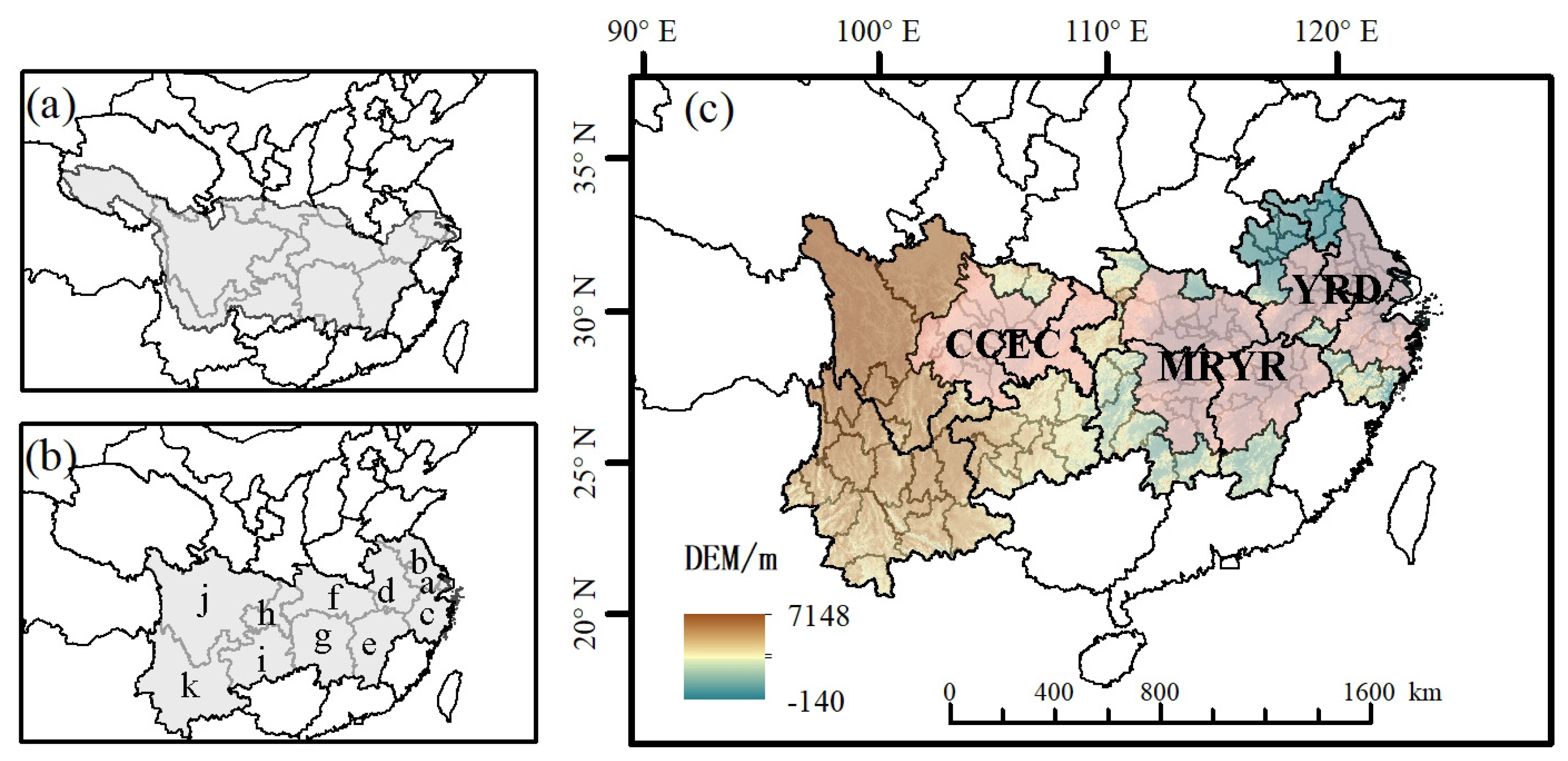
2.1. Study Area

The mainstream of the Yangtze River is more than 6300 km, with a basin area of 1.8 × 10⁶ km², accounting for about 1/5 of China’s total national land area (Figure 1a). The Yangtze River basin is extremely rich in natural resources, of which the total amount of water resources, biological resources, and mineral resources are among the top in China [20]. The Yangtze River is the largest river by discharge in China, with a total runoff of 9.6 × 10¹¹ m³, accounting for about 35% of the entire river runoff in China. Therefore, the Yangtze River is a critical wildlife habitat for China [21].

Unlike the Yangtze River basin (Figure 1a,b), the Yangtze River Economic Belt (YREB) is an important national development strategy zone, covering most of the regions of the Yangtze River basin and concluding Zhejiang Province [22]. The YREB covers 11 provincial administrative areas, i.e., Shanghai, Jiangsu, Zhejiang, Anhui, Jiangxi, Hubei, Hunan, Chongqing, Sichuan, Guizhou, and Yunnan. The Yangtze River Delta urban agglomeration (YRD), City clusters in the middle reaches of the Yangtze River (MRYR), and Chengdu-Chongqing economic circle (CCEC) are three national urban agglomerations in the YREB (Figure 1c). The YREB is a multi-stage ladder terrain, including mountains, plateaus, basins (tributaries), hills, and plains. The elevation of the YREB ranges from 140 to 7148 m. The average temperature in the YREB is about 15.8 °C; the temperature is decreasing from east to west. The annual average precipitation is about 1268 mm, increasing from northwest to southeast. Generally, the upstream of the YREB includes Sichuan, Yunnan, Guizhou, and Chongqing; the midstream of the YREB consists of Hubei, Hunan, and Jiangxi; the downstream of the YREB includes Jiangsu, Zhejiang, Anhui, and Shanghai [6].

2.2. Data Sources

The land-use/land-cover (LULC) maps are provided by the Climate Change Initiative (CCI, 300m resolution, http://maps.elie.ucl.ac.be/CCI/viewer/download.php, accessed on 10 November 2022). The precipitation, temperature, and solar radiation from 1999 to 2018, are provided by the National Meteorological Administration of China (http://data.cma.cn, accessed on 5 October 2022). The digital elevation model (DEM) data with 90 × 90 m spatial resolution is collected from the Resource and Environment Data Cloud Platform of China (http://www.resdc.cn/, accessed on 5 April 2019). Soil data, including soil types and root depth, is obtained from the China Soil Map, which is based on Harmonized World Soil Database provided by National Tibetan Plateau Data Center/Third Pole Environment Data Center (https://data.tpdc.ac.cn, accessed on 5 April 2019) [23]. The normalized difference vegetation index (NDVI) is gathered from the US National Oceanic and Atmospheric Administration (NOAA) Advanced Very High-Resolution Radiometer (AVHRR) (https://nex.nasa.gov, accessed on 10 November 2022). The night light data is observed from the Geographical Information Monitoring Cloud Platform (http://www.dsac.cn/DataProduct, accessed on 10 November 2022). The resolution of all spatial data has been resampled as 1000 × 1000 m for further ESs simulating process. The LULC, climatic, and geographic data are used to promote the InVEST model. The LULC, climatic, and vegetation data are applied to calculate the NPP. The night light data works as an indicator for analyzing the contribution of human activities.

3. Methods

3.1. Methodological Scheme

To detect the impact of human activities on the temporal and spatial changes of ESV in the YREB, this study selects GDP as the index to represent human activities, which have been inversed from the Night light Data [24,25]. The advantage of choosing the GDP rather than land use is that the GDP could not only describe the urbanization process but also reflect the intensity difference even in the same land use type [25]. Furthermore, four important water-related ESs, which are crucial for ecosystem stabilization and highly relied on water resources, have been simulated by the InVEST and CASA models, including water yield, soil retention, water purification, and NPP. The NPP represents the carbon fixation and oxygen release service [26]. The steps of this study are listed below: (1) first of all, the study period has been separated into two stages, the 1999–2008 and 2009–2018, for further research; (2) then, the selected ESs are simulated by InVEST and CASA model. Using the market and alternated market approach, the values for all ESs have been quantified, named integrated ESV; (3) finally, the correlation and attribution analysis are used to denote how the human activities would affect the ESV qualitatively and quantitatively.

3.1.1. CASA Model

The estimation of vegetation’s net primary productivity (NPP) is generally based on the CASA model [27]. This study uses the monthly precipitation, average temperature, radiation, and NDVI to estimate the NPP [28]. The primary calculation method is shown in the following equations:

$$NPP(x,t)=APAR(x,t)\times \epsilon (x,t)$$

(1)

where $APAR(x,t)$ represents the photosynthetic effective radiation (MJ/m²/month) absorbed by grid $x$ in month $t$, $\epsilon (x,t)$ represents the actual light energy utilization rate. The $\epsilon (x,t)$ is calculated by the CASA model, based on the vegetation types and climatic conditions.

$$APAR(x,t)=SOL(x,t)\times FPAR(x,t)\times 0.5$$

(2)

where $FPAR(x,t)$ represents the absorption ratio of the vegetation layer to the incident light and the effective radiation, and $SOL(x,t)$ represents the total solar radiation (MJ/m²/month) of the grid $x$ in month $t$. The $SOL(x,t)$ are acquired by the interpolated solar radiation distribution map, by using the climatic data sources.

$$FPAR(x,t)=\frac{\left(NDVI(x,t)-NDV{I}_{i,min}\right)\times \left(FPA{R}_{i,max}-FPA{R}_{i, min}\right)}{NDV{I}_{i,max}-NDV{I}_{i,min}}$$

(3)

where $NDV{I}_{i,max}$ and $NDV{I}_{i,min}$ are the maximum and minimum NDVI of the $i$th vegetation type, respectively. The $FPA{R}_{max}$ and $FPA{R}_{min}$ are identified as maximum and minimum $FPAR$ of the $i$th vegetation type, respectively, by the researchers referring to the relevant studies.

3.1.2. InVEST Model

The InVEST model is an open-source research tool widely used to quantify ESs functions and their values [29]. InVEST model mainly focuses on quantifying the value of various ESs and their spatial distribution, including water yield, soil retention, habitat quality, water purification, etc. Using its high-resolution computing characteristics, InVEST model can more intuitively reflect the spatial characteristics of ESV in macroecological environment research [9].

3.2. Quantification of ESs and Values

3.2.1. Water Yield

The principle of the water yield module of InVEST model is based on the estimation method of Budyko water heat coupling balance [30]. The simulation of the water yield module is based on the rainfall, potential evapotranspiration, land use, land cover, the available water content of vegetation, soil type, and other conditions. The results are output in grid units; the equations are listed below:

$$Y_{xj}=\left(1-\frac{AE{T}_{xj}}{P_x}\right)\times P_x$$

(4)

where, $Y_{xj}$ is the annual water yield of land type j in grid $x$ (mm·yr⁻¹); $AE{T}_{xj}$ is the actual evapotranspiration of land type $j$ in grid $x$ (mm·yr⁻¹); $P_x$ is the annual precipitation of grid $x$ (mm·yr⁻¹).

$$\frac{AE{T}_{xj}}{P_x}=\frac{1+{\omega }_x+R_{xj}}{1+{\omega }_x+R_{xj}+1/R_{xj}}$$

(5)

where, $\frac{AE{T}_{xj}}{P_x}$ is the ratio of actual evapotranspiration to rainfall, obtained by the Budyko method; $R_{xj}$ is the Budyko index of the $j$th land use type on grid $x$; ${\omega }_x$ is the ratio of vegetation storage and precipitation.

In this study, the economic value of water conservation is measured by the water price of urban residents. The evaluation method of ESV is shown below:

$$V_{wy,x}=A_j\times Y_{xj}$$

(6)

$$E_1=a\times \sum V_{wy,x}$$

(7)

where $A_j$ is the total area for land type $j$ (m²); $V_{wy,x}$ is the water conservation capacity of the grid $x$ (m³·yr⁻¹); $E_1$ is the ESV of water conservation for the study area (yuan); $a$ is the average water consumption price of residents (yuan/m³). In this study, the average water price of the first laddered of residents in major cities of the Yangtze River Economic Belt (Wuhan, Changsha, Guiyang, Nanchang, Chengdu, Nanjing, Shanghai, Chongqing, Hangzhou, Kunming, and Hefei) in 2018 is 3.01 yuan/m³, which is taken as the average water price of residents in the Yangtze River Economic Belt in the accounting method.

3.2.2. Soil Retention

The soil retention module describes the mechanism of slope soil erosion and the watershed sediment transport process [30]. The main principle is using the USLE (Universal Soil Loss Equation) to quantify the soil erosion degree in different regions, based on diverse terrain, landform, slope, soil, precipitation, and other conditions [31]. The difference between potential soil loss and actual soil loss is used to estimate the ES function of soil retention; the equation is listed below:

$$S{R}_x=R_x\times K_x\times L{S}_x-R_x\times K_x\times L{S}_x\times C_x\times P_x$$

(8)

where, $S{R}_x$ is the actual soil erosion of grid $x$ considering vegetation interception (tons·ha⁻¹·yr⁻¹); $R_x$ is rainfall erosivity (MJ·mm·ha⁻¹·h⁻¹·yr⁻¹), which is calculated by the precipitation in Equation (9) [32]; $K_x$ is soil erodibility (tons·ha·h·ha⁻¹·MJ⁻¹·mm⁻¹), which is calculated by the soil data in Equations (10)–(12) [33]; $L{S}_x$ is the slope length factor, which is calculated by DEM data; $C_x$ is the vegetation coverage factor and $P_x$ is the factor of soil retention measures, both areas identified by the researchers refer to the relevant studies.

$$R={{\displaystyle \sum }}_1^{12}\left(1.735\times {10}^{\lg \left(\frac{p_i{}^2}{p}\right)-0.8188}\right)$$

(9)

$$\begin{gathered} K_{EPIC}=\left\{0.2+0.3\exp \left[-0.0256\times sand\left(1-\frac{silt}{100}\right)\right]\right\}\times {\left(\frac{silt}{clay+silt}\right)}^{0.3} \\ \times \left[1-0.25\times \frac{C}{C+\exp \left(3.72-2.95\times C\right)}\right] \\ \times \left[1-0.75\times \frac{SN}{SN+\exp \left(22.9\times SN-5.51\right)}\right] \end{gathered}$$

(10)

$$SN=1-sand/100$$

(11)

$$K=\left(-0.01383+0.51575\times K_{EPIC}\right)\times 0.1317$$

(12)

where $p_i$ is the precipitation for the $i$ month (mm); the $p$ is the annual average precipitation (mm). The terms in Equations (10)–(12), including $sand$, $silt$, $clay$, and $OM$ are the coefficient in soil data sources.

Ouyang has found in his research that the economic benefits of soil conservation mainly come from the well-functioned ecosystem, which reduces the siltation effect of sediment in the upstream water on the downstream lakes and reservoirs [34]. The effect could reduce the risk of environmental problems such as drought and flood disasters due to the reduction of reservoir capacity, and its ESV can be calculated according to the following formula:

$$V_{soil}=\sum A_x\times S{R}_x$$

(13)

$$E_2=0.24\times V_{soil}\times \frac{T}{\rho }$$

(14)

where $V_{soil}$ is the total amount of soil retention (t); $A_x$ is the area for grid $x$ (ha); $E_2$ is the ESV of soil retention for the study area (yuan); $T$ is the construction cost per unit storage capacity of the reservoir (yuan/m³); $\rho$ is the soil bulk density (t/m³). In this study, the reservoir’s construction cost per unit capacity is taken as 6.11 yuan/m³ by referring to relevant studies.

3.2.3. Water Purification

The ecosystem has a self-regulation ability when disturbed and threatened by external factors to ensure that the ecological process can be carried out stably [30]. When the pollutants increase, elements in the ecosystem, including vegetation, animals, microorganisms, and soil, will intercept, adsorb, and even digest pollutants. The water purification module of InVEST model is used to evaluate the purification capacity of the ecosystem, the equations are listed below:

$$AL{V}_{\left(x\right)}=HS{S}_{\left(x\right)}·po{l}_{\left(x\right)}$$

(15)

where, $AL{V}_{\left(x\right)}$ is the adjusted output of grid $x$ (kg/ha); $HS{S}_{\left(x\right)}$ is the hydrological sensitivity score of grid $x$; $po{l}_{\left(x\right)}$ is the output coefficient of grid $x$, which is determined by the InVEST model, based on the land use types, topographic, and climatic conditions of the study area.

$$HS{S}_{\left(x\right)}=\frac{{\lambda }_x}{\overline{\lambda }w}$$

(16)

where, ${\lambda }_x$ is the runoff coefficient of each grid; $\overline{\lambda }w$ is the average runoff coefficient.

$${\mathrm{E}}_3=\left(ALV/{10}^3\right)\times 4.8\times {10}^4+\left(\mathrm{NPP}/{10}^3\right)\times 3.18\times {10}^4$$

(17)

The water purification function mainly targets the primary pollutants of non-point source pollution, nitrogen, and phosphorus. Referring to the treatment cost of nitrogen and phosphorus per unit weight of the lake, the treatment cost of nitrogen and phosphorus is set as 4.8 × 10⁴ yuan/ton and 3.18 × 10⁵ yuan/ton. Where ${\mathrm{E}}_3$ is the ESV of Water purification for the study area (yuan).

3.2.4. Net Primary Productivity

Carbon fixation and oxygen release come from the photosynthesis of vegetation [26]. In the study, NPP (net primary productivity of vegetation) is used to characterize the carbon fixation and oxygen release function of photosynthesis.

According to relevant research, it can be estimated that every 162 g of NPP can absorb 264 g of carbon dioxide and release 192 g of oxygen. The ESV can be calculated by comparing it with the cost of afforestation; that is, absorbing one ton of carbon dioxide will generate 260.9 yuan; Releasing one ton of oxygen generates a value of 352.93 yuan [35]. Where ${\mathrm{E}}_4$ is the ESV of NPP (yuan).

$${\mathrm{E}}_4=\left(\mathrm{NPP}/{10}^6\times \frac{264}{162}\right)\times 260.9+\left(\mathrm{NPP}/{10}^6\times \frac{192}{162}\right)\times 352.93$$

(18)

3.3. Statistical Methods

3.3.1. Correlation Analysis

Correlation analysis is the mathematical statistical analysis of two or more variables with a specific correlation [36]. The closeness between two or more variables is characterized by the value range of [−1, 1]. It should be noted that the correlation is not necessarily causal, and the variables for correlation analysis need to have a logical relationship in general cognition. In this study, the Spearman correlation analysis is selected as the primary method for correlation study. The main evaluation methods of the Spearman correlation coefficient are as follows:

$$\rho =1-\frac{6{{\displaystyle \sum }}_{i=1}^N{d}_i{}^2}{N\left(N-1\right)}$$

(19)

$$\rho =\frac{{{\displaystyle \sum }}_{i=1}^N(x_i-\overline{x})(y_i-\overline{y})}{\sqrt{{{\displaystyle \sum }}_{i=1}^N(x_i-\overline{x}{)}^2(y_i-\overline{y}{)}^2}}$$

(20)

where $\rho$ is the Spearman correlation coefficient; $d_i$ is the difference between the two sides of row i; N is the number of data lines; $x_i$ is the $x$ variable value of bit $i$; $\overline{x}$ is the average of $x$ variables; $y_i$ is the value of the y variable in bit $i$; $\overline{y}$ is the average value of $y$ variable.

3.3.2. Attribution Analysis

$$\Delta R_x={\epsilon }_x\frac{R}{x}\Delta x$$

(21)

where, $\Delta R_x$ is the impact of influencing factors on the change of ESs; $R$ is the ESs (water yield, soil retention, water purification, carbon fixation, and oxygen release); $x$ is an influencing factor; $\Delta x$ is the difference between the influencing factor and the reference value in the study period; ${\epsilon }_x$ is the elasticity coefficient [37].

$${\epsilon }_x=\frac{\left(R_i-\overline{R}\right)/\overline{R}}{\left(x_i-\overline{x}\right)/\overline{x}}$$

(22)

where, $R_i$ is the ESs of a certain year; $x_i$ is a certain influencing factor affecting ESV; $\overline{R}$ is the annual value of ESs; $\overline{x}$ is the annual value of an influencing factor during the study period [6].

$$\delta R_{hum}=\frac{\Delta R_x}{\Delta }\times 100\%$$

(23)

where, $\delta R_{hum}$ is the relevant value for the impact of human activities on ESs; $\Delta$ is the change of ESs.

4. Results and Discussion

4.1. Changing Environment in the Yangtze River Economic Belt

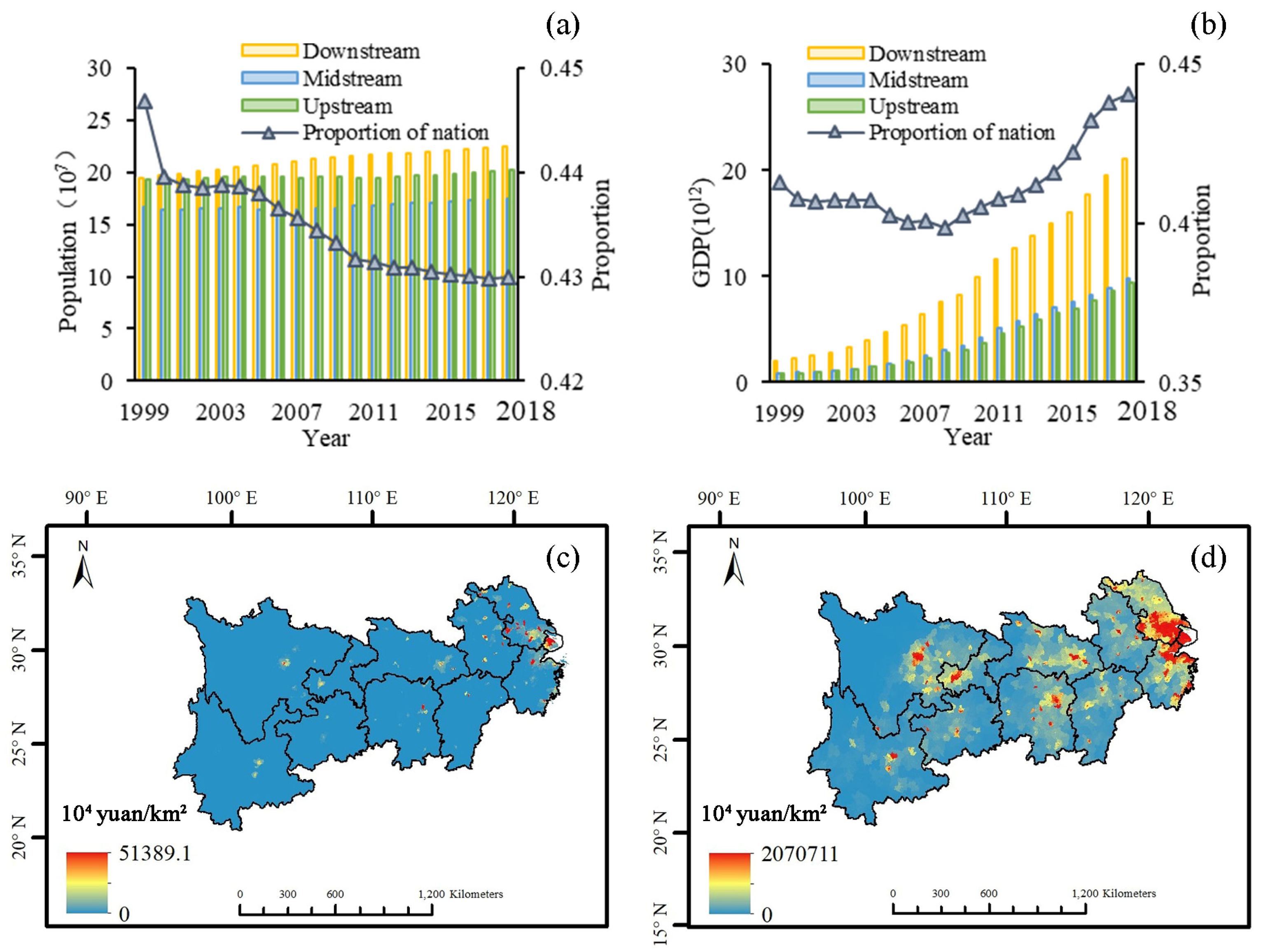
4.1.1. Social-Economic Development

During the study period, the economic aggregate of the YREB shows a steady upward trend, breaking through 1 × 10¹³ yuan in 2007, 2 × 10¹³ yuan in 2011, 3 × 10¹³ yuan in 2015, and 4 × 10¹³ yuan in 2018. The GDP is about 12 times in 2018 than in 1999, while the population accounts for about 43% of the total national population during the study period (Figure 2a,b). The proportion of the total economic output of the YREB in the whole nation presents a downward trend before 2008. After 2008, the proportion of the total economic output of the YREB rises rapidly from the lowest point of 39.86% in 2008 to 46.46% in 2018 of the whole nation, with an annual increase rate of 6.6%. Meanwhile, the overall economic situation of the YREB shows a stable growth trend. However, rapid economic development has accelerated the imbalance of regional development. From 2013 to 2018, the financial gap between the downstream of the YREB and the midstream increased at an annual growth rate of 6 × 10⁹ yuan. Of 11 provinces and cities in the YREB, Jiangsu indicates the highest average GDP for most of the years during the study period of about 4.42 trillion yuan, while Guizhou has the lowest average GDP of only 0.62 trillion yuan (Figure 2b).

The GDP of the downstream of the YREB is significantly higher than that of the midstream and upstream (Figure 2b). From 2009 to 2018, a social-economic radiating pattern is formed in the YRD from Shanghai to northern Jiangsu, southern Anhui, and Zhejiang [38]. Furthermore, the development of cities in the midstream and upstream of the YREB presents a cluster development trend driven by the growth of provincial capital cities. During the study period, the provincial capitals of the YREB gradually came to play a leading role in driving the rapid development of surrounding cities (Figure 2c,d). The strategic layout of the YRD, MRYR, and CCEC has significantly promoted the coordinated development of the YREB (Figure 1c) [39]. However, it can also be found that the economic and social development in the southwest, northwest, and south-central regions of the YREB, which are responsible for ecological environment protection and ecosystem diversity maintenance, is still lagging.

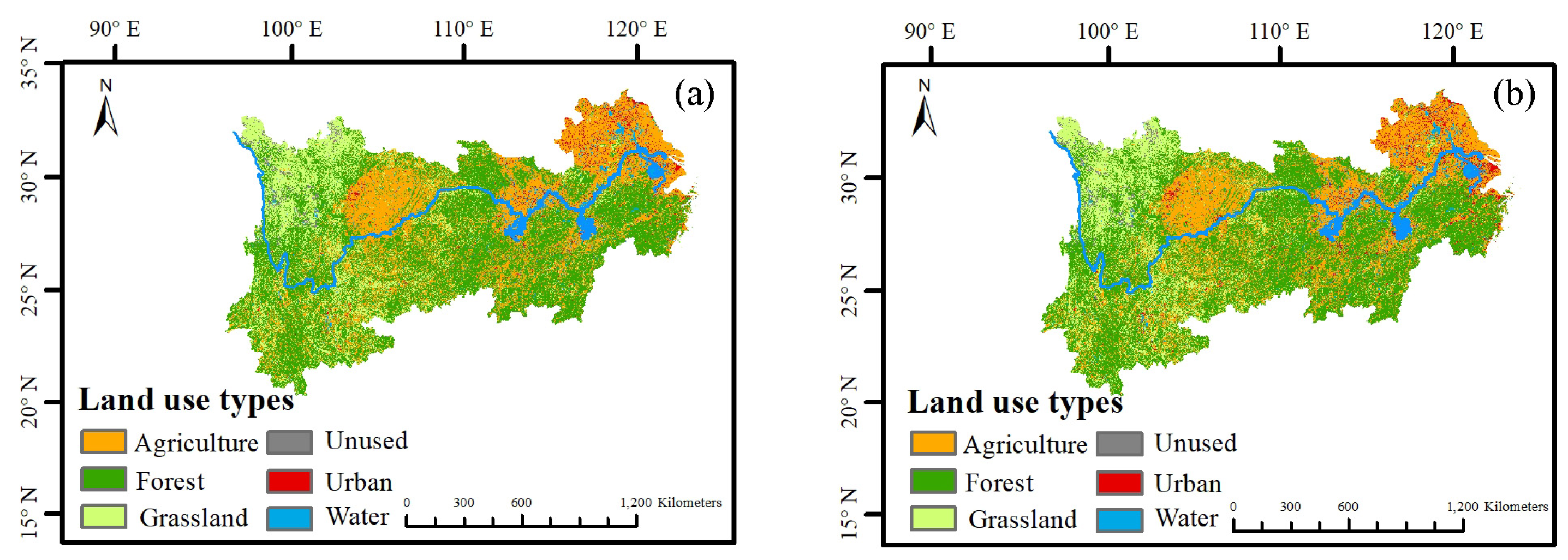
4.1.2. Land Use Land Cover Change

Due to the different functional positioning and development pace, the land use and land cover distribution characteristics are quite different around the YREB. The characteristics of rapid economic and social development of the downstream of the YREB can be noticed from the proportion of the increase in urban expansion. Owing to important ecological barrier orientation, the upstream and midstream are covered by important forests, grassland, wetland, and biodiversity conservation area (Figure 3a,b).

In the YREB, the forest and grassland accounted for more than 40% and 16%, respectively, in both 1999 and 2018. Different from the upstream and midstream, the downstream works as an essential engine of China’s economic and social development, though the downstream has the smallest area in the YREB. The urban area in the downstream accounts for the highest proportion of the YREB during the study period (more than 1.5%). It is worth noting that the agricultural area in the upstream accounts for more than 13%, while the urban area only accounts for about 0.5% in the YREB (

Table 1. The proportion of land use in the upstream, midstream, and downstream in the YREB.

(km2)	1999			2018
	Upstream	Midstream	Downstream	Upstream	Midstream	Downstream
Agricultural	13.55%	8.62%	9.10%	13.29%	8.40%	8.62%
Forest	24.81%	16.06%	5.02%	24.88%	15.98%	4.97%
Grassland	14.94%	1.07%	0.56%	14.84%	1.06%	0.56%
Water	0.39%	1.21%	1.09%	0.45%	1.28%	1.11%
Urban	0.30%	0.51%	1.50%	0.53%	0.78%	2.00%
Unused	0.96%	0.10%	0.00%	0.97%	0.09%	0.00%

). This may be because the urban expansion is relatively limited, due to the hilly landform in the upstream. Most residents still rely on agricultural production upstream, which makes the overall economic and social development slower than the downstream (Figure 2c,d).

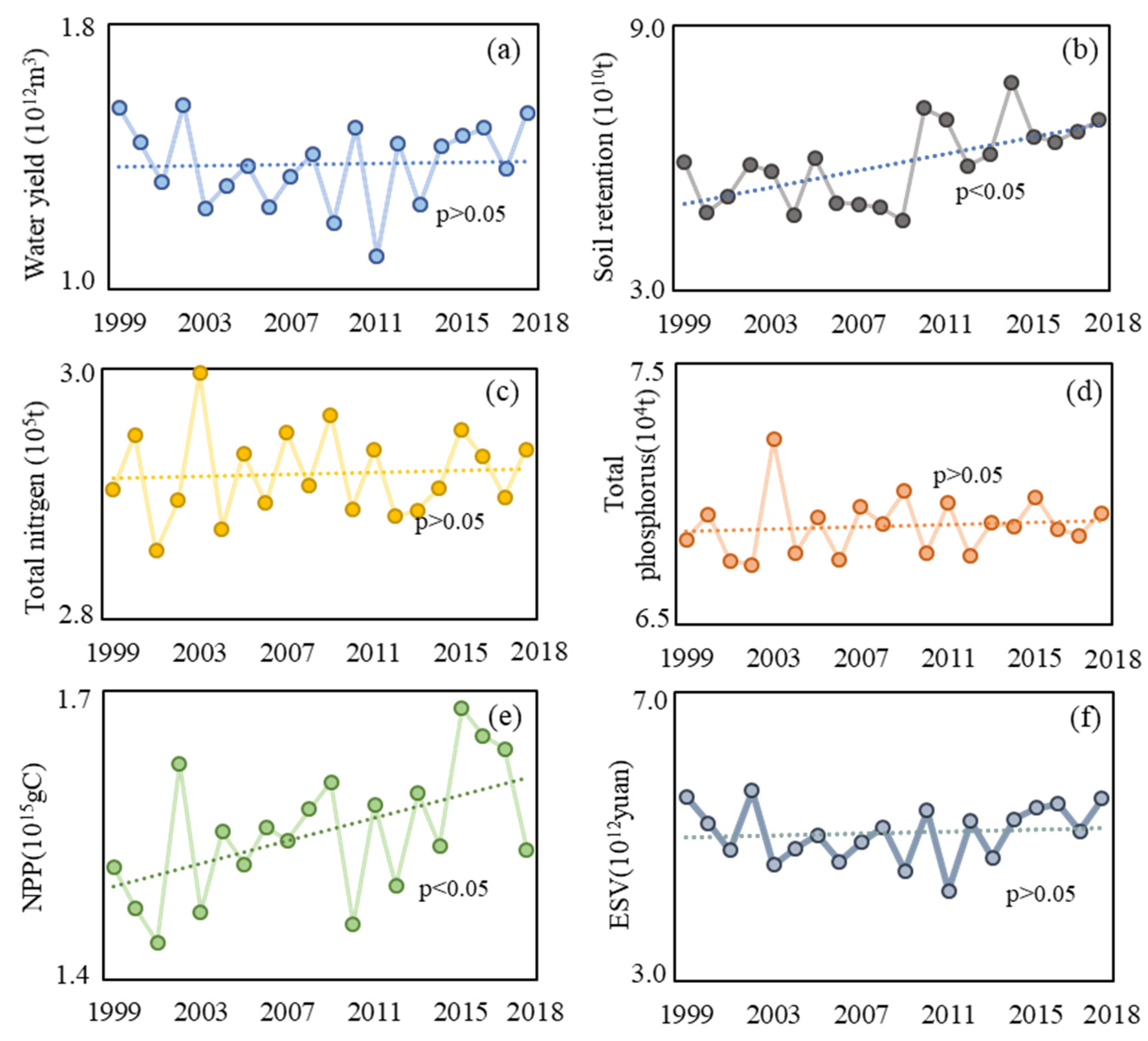
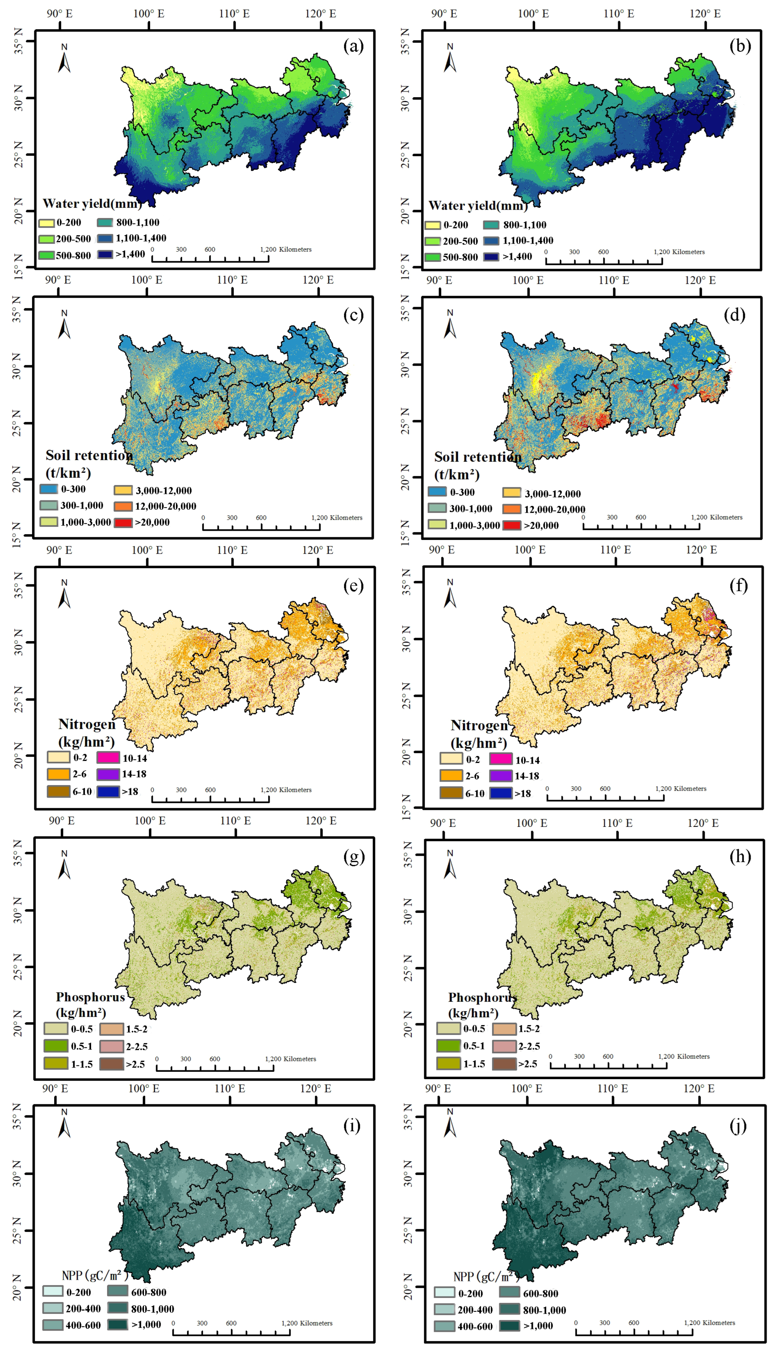
4.2. Changes of ESs and ESV

4.2.1. Water Yield

From 1999 to 2018, the water yield capacity of the YREB has shown a “U” shape change trend. The lowest water yield capacity is in 2011, with 1.11 × 10¹² m³. The highest water yield capacity is in 2002, with 1.56 × 10¹² m³ (Figure 4a). The previous study proves that the overall change trend of water yield is highly consistent with the precipitation change characteristics in the YREB [18]. The water yield capacity of the southern area of the YREB is higher than the northern area, and the proportion for the area of high annual water yield area (water yield > 1100 mm) becomes larger from 2009 to 2018 than from 1999 to 2008. From 1999 to 2008, the area of high annual water yield area accounted for 10.1% of the YREB, while from 2009 to 2018, the proportion is 21.4% (Figure 5a,b), which indicates that one-fourth of the regions in the YREB have plenty of water resources. Specifically, Zhejiang, Jiangxi, Hunan, and southern Yunnan present most higher water yield capacity, while Jiangsu, Anhui, Hubei, Chongqing, and Sichuan are relatively low.

4.2.2. Soil Retention

The soil retention of the YREB has significantly improved from 1999 to 2018. The soil retention reaches lowest in 1999, with 6.40 × 10¹⁰ t, while the highest soil retention appears in 2015, which raised 17.5% compared to 1999 (Figure 4b). The improvement of soil retention is closely related to the growth of vegetation in the YREB, during the study period [40]. Previous studies proved that soil retention is closely related to land use type, precipitation, topography, and other factors [41]. Taking the land use type as an example, studies show that the soil retention of forest land is the highest, compared to all other land use types. Therefore, the areas with high soil retention in the YREB are mainly concentrated in the high vegetation coverage areas in the upstream of the YREB, including Southeast Guizhou, Southwest Yunnan, Southwest Sichuan, South Zhejiang, and South Jiangxi. However, though the northwest of the YREB is dominated by forest and grassland, the steep mountains may be one of the main causes for the relatively low soil retention ability. Compared with 1999–2008, the areas with high soil retention (soil retention capacity > 20,000 t/km²) in 2009–2018 have shown an enhancement and expansion trend, which is also mutually corroborated with the research conclusion of the vegetation well growth in the YREB (Figure 5c,d).

4.2.3. Water Purification

Rapid urbanization has increased the pressure on non-point source pollution prevention in provinces and cities in the YREB [42]. However, according to the annual changes in total nitrogen and phosphorus output analysis, the YREB shows a fluctuating upward trend without significance. The pollution output reaches its peak in 2003 for total nitrogen and phosphorus. The corresponding output of total nitrogen and total phosphorus is 2.91 × 10⁶ t and 7.22 × 10⁵ t, respectively (Figure 4c,d). The output of total nitrogen and phosphorus in the YREB is mainly distributed in the YRD, MRYR, and CCEC (Figure 5e,f). The spatial difference between total nitrogen and phosphorus output are similar in the YREB during the past 20 years. The slight difference may be owing to the different interception efficiency of nitrogen and phosphorus by vegetation and various land use types (some studies show that the interception and absorption capacity of nitrogen by vegetation is stronger than that of phosphorus), the migration distance and coverage of phosphorus are slightly smaller than nitrogen [43]. However, due to the output of nitrogen and phosphorus being closely related to the land use type, the hot spots of nitrogen and phosphorus output have changed with the urbanization process [44]. For example, the output of nitrogen and phosphorus in Shanghai and surrounding cities present an upward trend year by year. In 1999–2008 and 2009–2018, the output of nitrogen and phosphorus in the north of Jiangsu and Anhui Province tended to decrease, which may be caused by the transition of some agricultural areas with highly non-point source pollution to the urban area with low pollution loads. From 1999 to 2008, the area with a high output of nitrogen and phosphorus (total nitrogen > 10 kg/hm², total phosphorus > 1.5 kg/hm²) accounted for about 0.4% of the YREB, while the area accounted for about 1.8% of the YREB during 2009–2018 (Figure 5g,h).

4.2.4. Net Primary Productivity

During the study period, the NPP of the YREB has also significantly increased [45]. The lowest NPP is observed in 1999, with 1.52 × 10¹⁵ gC, while the highest NPP has presented in 2015, with 1.68 × 10¹⁵ gC, which has raised 11% (Figure 4e). NPP is determined by many causes, the vegetation type and climate conditions are the two most important factors. Spatially, the NPP of the YREB shows a decreasing trend from southwest to northeast, which has shown a similar change trend with the stepped landform characteristics of the YREB. The high NPP (NPP > 1000 gC/m²) areas in the YREB are mainly concentrated in the south of Yunnan and the southwest of Sichuan (Figure 5i,j). These areas are also the location of important primeval forests and nature reserves in China. Adequate protection and suitable climatic conditions make vegetation proliferate. From 2009 to 2018, the high NPP areas in the midstream and the southwest describes a shrinking trend. Considering the results of the previous water yield simulation, the weak growth of vegetation may be suppressed due to the lack of precipitation in this period.

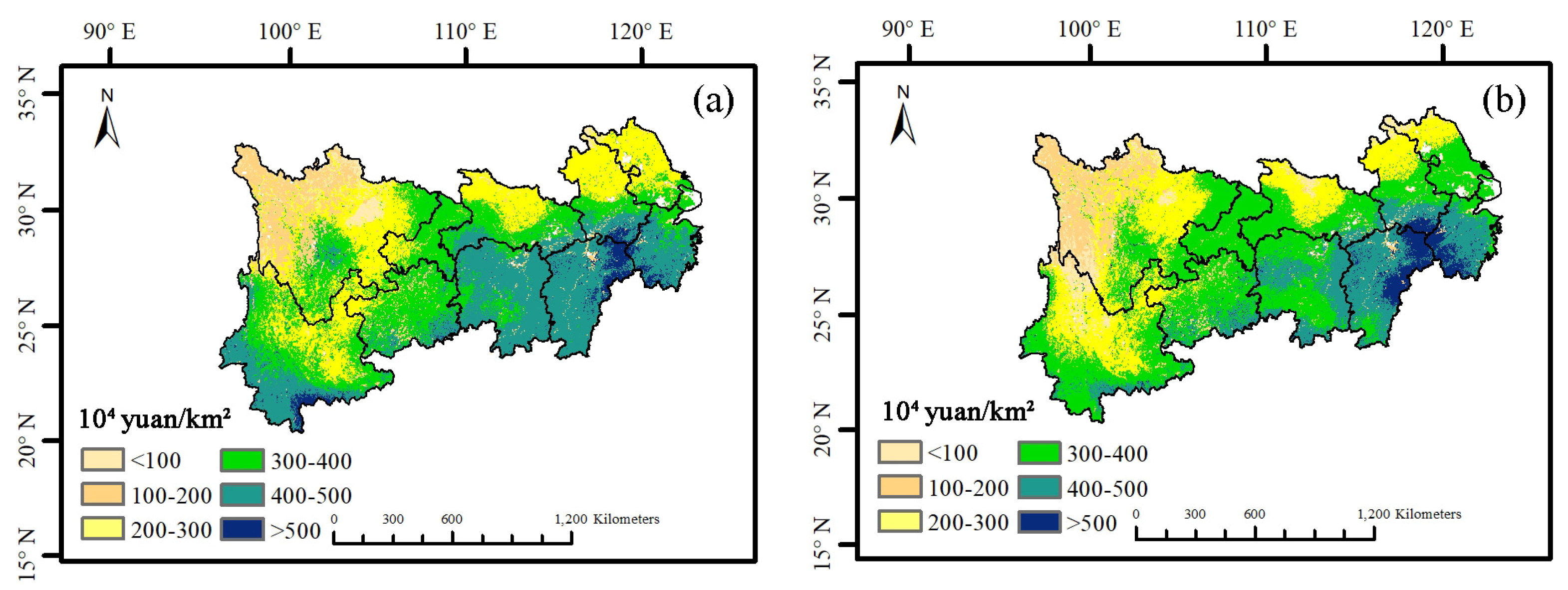
4.2.5. Integrated ESV

The integrated ESV of the YREB presents no significant change trend between 1999–2018 [18]. The integrated ESV become lower in 2003–2012, while raise higher in 1999–2002 and 2016–2018. The lowest integrated ESV is 4.26 × 10¹² yuan in 2011, while the highest is 5.63 × 10¹² yuan in 2002 (Figure 4f). Different from the current studies, which are based on land use types and parameters, rather than ecological processes. This study uses ecological models and considers more characteristics of annual changes in climate, topographic, and geomorphic factors, etc. Therefore, the results of this study showed a slight difference in spatial distribution for integrated ESV(Figure 6). For the studies based on land use types, the distribution characteristics of the integrated ESV in the YREB are decreasing from northwest to east, while, the spatial distribution characteristics of the integrated ESV in this study are generally more prominent in the south than in the north, and decreasing from southeast to northwest [46]. These differences may be due to the complicated landform for mountains with large slopes and lower precipitation [47,48].

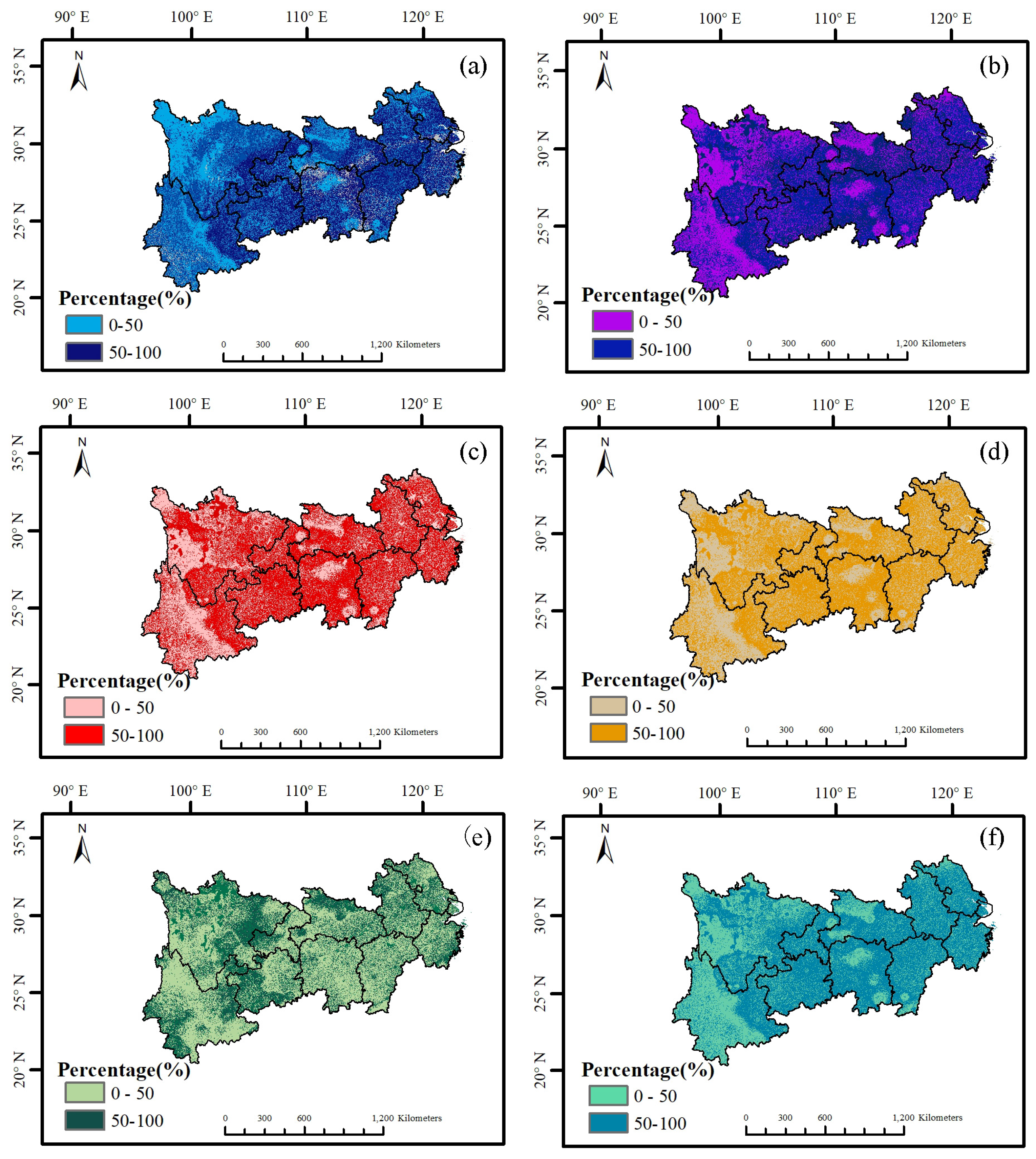
4.3. Identification of Driving Factors

4.3.1. The Correlated Relation between Human Activities to ESs and ESV

Though a strong positive correlation between the ESV of water yield and human activities have been identified in northern Guizhou, southern Chongqing, and southern Hubei provinces, most of the area in the YREB have presented a negative correlation [49,50], such as the northwest mountain area of Sichuan, and the junction of Jiangxi, Zhejiang, and the Anhui provinces. The mountain area in the northwest of Sichuan and the junction of Jiangxi, Zhejiang, and Anhui provinces showed a relatively obvious negative correlation. A strong positive correlation has been identified between northern Guizhou, southern Chongqing, and southern Hubei. It can be inferred that to achieve the protection and promotion of ESV in northwest Sichuan, strong constraints on human activities need to be imposed (Figure 7a). Soil retention is negatively correlated with human activities [51]. The primary influence factor of human activities on soil retention is agricultural activities. Therefore, soil retention is strongly negatively correlated with human activities, which are covered by large agricultural areas, such as Sichuan Basin and northern Jiangsu. Accordingly, vegetation can improve soil retention by reducing runoff and limiting erosion. In Guizhou, Yunnan, and Chongqing, the soil retention in the forest areas has not been interrupted by limited human activities, which may indicate that when carrying out the national park strategies, the conservation area can improve the soil retention services without relocating the residents to other regions (Figure 7b). The regions with a negative correlation between water purification and human activities coincide with the hot spots of the economic and social development area in the YREB. The YRD, MRYR, and CCEC all present obvious negative correlations with the water purification value (Figure 7c,d). To meet the requirements of high-quality life, natural landscape space has been compressed by the construction area and agricultural area in these urban agglomerations [52]. Urban non-point source pollution and agricultural non-point source pollution have intensified, leading to the reduction of ecosystem resilience. Consistent with the conclusion that human activities will affect vegetation growth, human activities in CCEC are negatively related to NPP. In addition, human activities are positively related to NPP in provinces and cities with large areas of virgin forests, such as western Sichuan and Yunnan, and Guizhou (Figure 7e). These findings express that in areas with fewer human activities and covered mainly by forest, the limited and regular human activities will not affect the ESV of vegetation. In some regions of the YREB, the correlation between NPP and human activities are different from the traditional research. About half of the City clusters in the middle reaches of the Yangtze River and the Yangtze River Delta urban agglomeration have shown a positive correlation between human activities and NPP. These results can be concluded that the uncertainty of climate change may mitigate the negative effect carried by human activities [53].

Overall, human activities have a strong correlation with the integrated ESV. For example, human activities in northern Guizhou and Yunnan provinces strongly correlate with the integrated ESV (Figure 7f), however, the Southwest Sichuan, CCEC, and the south of the YRD show a strong negative correlation.

4.3.2. The Attribution of Human Activities on ESs and ESV Change

The main human activity-influenced areas are gradually concentrated from 1999–2018. During the study period, the main influenced areas cover the eastern, central, and central YREB. The impact of human activities in all provinces has exceeded 50% (Figure 8f,

Table 2. The contribution rate of climate change and human activities to ESV in the YREB during 2009–2018 than in 1999–2008.

	ESV	Water Yield	Soil Retention	Total Nitrogen	Total Phosphorus	NPP
Zhejiang	67	57	61	61	61	39
Jiangsu	62	59	61	58	58	36
Anhui	60	56	62	61	61	41
Shanghai	61	49	62	62	62	39
Jiangxi	64	55	63	61	61	38
Hunan	67	56	66	65	65	33
Hubei	63	61	61	61	61	38
Sichuan	54	58	51	49	49	44
Yunnan	52	52	47	61	47	48
Chongqing	63	60	63	58	63	37
Guizhou	62	60	56	61	57	35

). These findings emphasize that restricting and managing human activities is crucial for the environmental protection approaches, which will significantly affect the health of the ecosystem in the future.

Similar to the main influenced areas, the areas where water yield changes are mainly affected by human activities are consistent with the urban expansion region. The land use change and the urbanization process of cities have considerably changed the pattern of the ecological environment around cities and towns. Therefore, the attribution of human activities to the water yield in the YRD, MRYR, and CCEC ranges from 65% to 100% (Table 2). In the west of the YREB, human activities in Yunnan and Sichuan are not the main factors affecting the water yield (Figure 8a). As for soil retention, human activities in the YREB have always been the main factor, though the spatial distribution is quite different upstream, midstream, and downstream. The regions where human activities showed 0–50% attribution are mainly located in vegetation-covered areas, including northwest Sichuan, southwest Yunnan, south Hubei, and north Hunan. The other regions, where human activities have attributed 60–100%, are mainly concentrated in three urban agglomerations (Figure 8b). This result suggests that the land use change in the YREB has dramatically converted the spatial distribution of soil retention. Similarly, the spatial distribution of the regions whose total nitrogen/phosphorus are mainly affected by human activities is also consistent with the trend of social development in the YREB (Figure 8c,d). It is significant, although the development of urban agglomerations and the economic and social development of the YREB have encroached on a natural environment, the disturbance of human activities on NPP has not exceeded 50%. This result may suggest that human activities are not the main influencing factor for NPP in the YREB (Figure 8e, Table 2). Therefore, the other mitigating factors may be prominent for vegetation growth, including environmental protection policies, climate change, and tree planting actions [54].

5. Limitations and Uncertainties

The input ecological vegetation coefficient parameters of InVEST model, which is used to evaluate the ESs, have been intercalated as the same value. However, the vegetation in regions would present different ecological functions [55]. Therefore, further studies on InVEST model could focus on providing a module for researchers to define the vegetation coefficient parameters for the same vegetation type in different regions when conducting the large-scale simulation. Moreover, this study provides a hypothesis that human activities are not the main factor for NPP in the YREB, which may need more discussion in the future, such as detecting the contribution of human activities on ESV by industries, conducting the policies studies to evaluate the possible influence for policies on ESV change, and exploring more statistical and physical methods to seek how climate, social, policy, and other possible factors could affect the ESV.

6. Conclusions

This study identifies the impact of human activities on the temporal and spatial changes of ESV (water yield, soil retention, water purification, NPP, and integrated ESV) in the YREB, China, using the InVEST model, CASA model, and statistical methods. The results demonstrate that though the land use change and human activities have vastly intensified, the integrated ESV in YREB has not presented a significant change trend, the average ESV is 5.06 × 10¹² yuan during 1999–2018. The overall water yield change trend is highly consistent with the precipitation change characteristics and is weakly negatively correlated with human activities. The soil retention of the YREB is significantly improved from 1999 to 2018, while human activities have always been the main factor and shown a negative correlation. The output of total nitrogen and phosphorus in the YREB is mainly distributed in the YRD, MRYR, and CCEC with no noticeable interannual spatial difference during the study period. The NPP of the YREB increases significantly, although the urbanization process has encroached on the amount of specific natural environment areas. The disturbance of human activities on vegetation growth has not exceeded 50% for all the provinces and cities, which may indicate that the environmental protection policies and action, as well as the climate change, could support the YREB to become green. Our findings provide important information to inform policymakers to realize how the ESV changed in the YREB, and where need to draw more attention to realize the sustainable ESV and human wellbeing.

References

1. Daily, G.C. Nature’s Services: Societal Dependence On Natural Ecosystems; Island Press: Washington, DC, USA, 2012; ISBN 9781597267755. [Google Scholar]
2. Daily, G.C. Restoring Value to the World’s Degraded Lands. Science 1995, 269, 350–354. [Google Scholar] [CrossRef]
3. Costanza, R.; d’Arge, R.; Groot, R.d.; Farber, S.; Grasso, M.; Hannon, B.; Limburg, K.; Naeem, S.; O’Neill, R.V.; Paruelo, J.; et al. The value of the world’s ecosystem services and natural capital. Nature 1997, 387, 253–260. [Google Scholar] [CrossRef]
4. Wu, Y.; Xu, Y.; Yin, G.; Zhang, X.; Li, C.; Wu, L.; Wang, X.; Hu, Q.; Hao, F. A collaborated framework to improve hydrologic ecosystem services management with sparse data in a semi-arid basin. Hydrol. Res. 2021, 52, 1159–1172. [Google Scholar] [CrossRef]
5. Burkhard, B.; Kroll, F.; Nedkov, S.; Müller, F. Mapping ecosystem service supply, demand and budgets. Ecol. Indic. 2012, 21, 17–29. [Google Scholar] [CrossRef]
6. Xu, Y.; Wu, Y.; Zhang, X.; Yin, G.; Fu, Y.; Wang, X.; Hu, Q.; Hao, F. Contributions of climate change to eco-compensation identification in the Yangtze River economic Belt, China. Ecol. Indic. 2021, 133, 108425. [Google Scholar] [CrossRef]
7. Caro, C.; Marques, J.C.; Cunha, P.P.; Teixeira, Z. Ecosystem services as a resilience descriptor in habitat risk assessment using the InVEST model. Ecol. Indic. 2020, 115, 106426. [Google Scholar] [CrossRef]
8. Li, M.; Liang, D.; Xia, J.; Song, J.; Cheng, D.; Wu, J.; Cao, Y.; Sun, H.; Li, Q. Evaluation of water conservation function of Danjiang River Basin in Qinling Mountains, China based on InVEST model. J. Environ. Manag. 2021, 286, 112212. [Google Scholar] [CrossRef] [PubMed]
9. Dennedy-Frank, P.J.; Muenich, R.L.; Chaubey, I.; Ziv, G. Comparing two tools for ecosystem service assessments regarding water resources decisions. J. Environ. Manag. 2016, 177, 331–340. [Google Scholar] [CrossRef] [PubMed] [Green Version]
10. Wang, Y.; Ye, A.; Peng, D.; Miao, C.; Di, Z.; Gong, W. Spatiotemporal variations in water conservation function of the Tibetan Plateau under climate change based on InVEST model. J. Hydrol. Reg. Stud. 2022, 41, 101064. [Google Scholar] [CrossRef]
11. He, J.; Zhao, Y.; Wen, C. Spatiotemporal Variation and Driving Factors of Water Supply Services in the Three Gorges Reservoir Area of China Based on Supply-Demand Balance. Water 2022, 14, 2271. [Google Scholar] [CrossRef]
12. Yang, R.; Ren, F.; Xu, W.; Ma, X.; Zhang, H.; He, W. China’s ecosystem service value in 1992-2018: Pattern and anthropogenic driving factors detection using Bayesian spatiotemporal hierarchy model. J. Environ. Manag. 2022, 302, 114089. [Google Scholar] [CrossRef]
13. Yuan, J.; Li, R.; Huang, K. Driving factors of the variation of ecosystem service and the trade-off and synergistic relationships in typical karst basin. Ecol. Indic. 2022, 142, 109253. [Google Scholar] [CrossRef]
14. Wang, Y.; Shataer, R.; Zhang, Z.; Zhen, H.; Xia, T. Evaluation and Analysis of Influencing Factors of Ecosystem Service Value Change in Xinjiang under Different Land Use Types. Water 2022, 14, 1424. [Google Scholar] [CrossRef]
15. Song, F.; Su, F.; Mi, C.; Sun, D. Analysis of driving forces on wetland ecosystem services value change: A case in Northeast China. Sci. Total Environ. 2021, 751, 141778. [Google Scholar] [CrossRef] [PubMed]
16. Xu, X.; Yang, G.; Tan, Y.; Liu, J.; Hu, H. Ecosystem services trade-offs and determinants in China’s Yangtze River Economic Belt from 2000 to 2015. Sci. Total Environ. 2018, 634, 1601–1614. [Google Scholar] [CrossRef]
17. Li, D.; Zhang, J. Measurement and analysis of ecological pressure due to industrial development in the Yangtze River economic belt from 2010 to 2018. J. Clean. Prod. 2022, 353, 131614. [Google Scholar] [CrossRef]
18. Feng, Z.; Jin, X.; Chen, T.; Wu, J. Understanding trade-offs and synergies of ecosystem services to support the decision-making in the Beijing–Tianjin–Hebei region. Land Use Policy 2021, 106, 105446. [Google Scholar] [CrossRef]
19. Vaz, A.S.; Amorim, F.; Pereira, P.; Antunes, S.; Rebelo, H.; Oliveira, N.G. Integrating conservation targets and ecosystem services in landscape spatial planning from Portugal. Landsc. Urban Plan. 2021, 215, 104213. [Google Scholar] [CrossRef]
20. Xu, X.; Pan, L.-C.; Ni, Q.-H.; Yuan, Q.-Q. Eco-efficiency evaluation model: A case study of the Yangtze River Economic Belt. Environ. Monit. Assess. 2021, 193, 457. [Google Scholar] [CrossRef]
21. Chen, Z.; Li, J.; Shen, H.; Zhanghua, W. Yangtze River of China: Historical analysis of discharge variability and sediment flux. Geomorphology 2001, 41, 77–91. [Google Scholar] [CrossRef]
22. Tian, Y.; Sun, C. Comprehensive carrying capacity, economic growth and the sustainable development of urban areas: A case study of the Yangtze River Economic Belt. J. Clean. Prod. 2018, 195, 486–496. [Google Scholar] [CrossRef]
23. Liu, F.; Zhang, G. Basic Soil Property Dataset of High-Resolution China Soil Information Grids (2010–2018); National Tibetan Plateau/Third Pole Environment Data Center: Nanjing, China, 2021. [Google Scholar] [CrossRef]
24. Wu, J.; Wang, Z.; Li, W.; Peng, J. Exploring factors affecting the relationship between light consumption and gdp based on dmsp/ols nighttime satellite imagery. Remote Sens. Environ. 2013, 134, 111–119. [Google Scholar] [CrossRef]
25. Zhong, Y.; Lin, A.; Xiao, C.; Zhou, Z. Research on the Spatio-Temporal Dynamic Evolution Characteristics and Influencing Factors of Electrical Power Consumption in Three Urban Agglomerations of Yangtze River Economic Belt, China Based on DMSP/OLS Night Light Data. Remote Sens. 2021, 13, 1150. [Google Scholar] [CrossRef]
26. Zhang, T.; Cao, G.; Cao, S.; Zhang, X.; Zhang, J.; Han, G. Dynamic assessment of the value of vegetation carbon fixation and oxygen release services in qinghai lake basin. Acta Ecol. Sin. 2016, 37, 79–84. [Google Scholar] [CrossRef]
27. Potter, C.S.; Randerson, J.T.; Field, C.B.; Matson, P.A.; Vitousek, P.M.; Mooney, H.A.; Klooster, S.A. Terrestrial ecosystem production: A process model based on global satellite and surface data. Glob. Biogeochem. Cycles 1993, 7, 811–841. [Google Scholar] [CrossRef]
28. Ruimy, A.; Saugier, B.; Dedieu, G. Methodology for the estimation of terrestrial net primary production from remotely sensed data. J. Geophys. Res. 1994, 99, 5263. [Google Scholar] [CrossRef]
29. Wang, Y.; Bakker, F.; de Groot, R.; Wörtche, H. Effect of ecosystem services provided by urban green infrastructure on indoor environment: A literature review. Build. Environ. 2014, 77, 88–100. [Google Scholar] [CrossRef]
30. Sharp, R.; Douglass, J.; Wolny, S.; Arkema, K.; Bernhardt, J.; Bierbower, W.; Chaumont, N.; Denu, D.; Fisher, D.; Glowinski, K.; et al. InVEST User’s Guide 3.9; The Natural Capital Project: Stanford, CA, USA, 2017. [Google Scholar]
31. Renard, K.G.; Freimund, J.R. Using monthly precipitation data to estimate the R-factor in the revised USLE. J. Hydrol. 1994, 157, 287–306. [Google Scholar] [CrossRef]
32. Wischmeier, W.H.; Smith, D.D. Rainfall energy and its relationship to soil loss. Trans. Am. Geophys. Union 1958, 39, 285–291. [Google Scholar] [CrossRef]
33. Jones, C.A.; Dyke, P.T.; Williams, J.R.; Benson, V.W.; Griggs, R.H. EPIC: An operational model for evaluation of agricultural sustainability. Agric. Syst. 1991, 37, 341–350. [Google Scholar] [CrossRef]
34. Ouyang, Z.; Wang, R.; Zhao, J. Ecosystem services and their economic valuation. Chin. J. Appl. Ecol. 1999, 10, 635. [Google Scholar]
35. He, Q.; Zeng, C.; Xie, P.; Liu, Y.; Zhang, M. An assessment of forest biomass carbon storage and ecological compensation based on surface area: A case study of Hubei Province, China. Ecol. Indic. 2018, 90, 392–400. [Google Scholar] [CrossRef]
36. Myers, L.; Sirois, M.J. Spearman Correlation Coefficients, Differences Between; John Wiley & Sons, Inc: Hoboken, NJ, USA, 2004. [Google Scholar]
37. Zheng, H.; Zhang, L.; Zhu, R.; Liu, C.; Sato, Y.; Fukushima, Y. Responses of streamflow to climate and land surface change in the headwaters of the Yellow River Basin. Water Resour. Res. 2009, 45, W00A19. [Google Scholar] [CrossRef]
38. Zhao, J.; Zhu, D.; Cheng, J.; Jiang, X.; Lun, F.; Zhang, Q. Does regional economic integration promote urban land use efficiency? Evidence from the Yangtze River Delta, China. Habitat Int. 2021, 116, 102404. [Google Scholar] [CrossRef]
39. Yang, Z. Comparison and empirical analysis of the urban economic development level in the Yangtze River urban agglomeration based on an analogical ecosystem perspective. Ecol. Inform. 2021, 64, 101321. [Google Scholar] [CrossRef]
40. Chen, D.; Jiang, P.; Li, M. Assessing potential ecosystem service dynamics driven by urbanization in the Yangtze River Economic Belt, China. J. Environ. Manag. 2021, 292, 112734. [Google Scholar] [CrossRef] [PubMed]
41. Wang, H.; Wang, W.J.; Liu, Z.; Wang, L.; Zhang, W.; Zou, Y.; Jiang, M. Combined effects of multi-land use decisions and climate change on water-related ecosystem services in Northeast China. J. Environ. Manag. 2022, 315, 115131. [Google Scholar] [CrossRef]
42. Xue, J.; Wang, Q.; Zhang, M. A review of non-point source water pollution modeling for the urban-rural transitional areas of China: Research status and prospect. Sci. Total Environ. 2022, 826, 154146. [Google Scholar] [CrossRef] [PubMed]
43. Wang, M.; Gong, Y.; Lafleur, P.; Wu, Y. Patterns and drivers of carbon, nitrogen and phosphorus stoichiometry in Southern China’s grasslands. Sci. Total Environ. 2021, 785, 147201. [Google Scholar] [CrossRef]
44. Zhao, Q.; Wang, Q. Water Ecosystem Service Quality Evaluation and Value Assessment of Taihu Lake in China. Water 2021, 13, 618. [Google Scholar] [CrossRef]
45. Chen, C.; Park, T.; Wang, X.; Piao, S.; Xu, B.; Chaturvedi, R.K.; Fuchs, R.; Brovkin, V.; Ciais, P.; Fensholt, R.; et al. China and India lead in greening of the world through land-use management. Nat. Sustain. 2019, 2, 122–129. [Google Scholar] [CrossRef]
46. Luo, Q.; Zhou, J.; Li, Z.; Yu, B. Spatial differences of ecosystem services and their driving factors: A comparation analysis among three urban agglomerations in China’s Yangtze River Economic Belt. Sci. Total Environ. 2020, 725, 138452. [Google Scholar] [CrossRef] [PubMed]
47. Diao, C.; Liu, Y.; Zhao, L.; Zhuo, G.; Zhang, Y. Regional-scale vegetation-climate interactions on the Qinghai-Tibet Plateau. Ecol. Inform. 2021, 65, 101413. [Google Scholar] [CrossRef]
48. Wu, Y.; Zhang, X.; Li, C.; Xu, Y.; Yin, G. Ecosystem service trade-offs and synergies under influence of climate and land cover change in an afforested semiarid basin, China. Ecol. Eng. 2020, 159, 106083. [Google Scholar] [CrossRef]
49. Wang, H.; Zhou, S.; Li, X.; Liu, H.; Chi, D.; Xu, K. The influence of climate change and human activities on ecosystem service value. Ecol. Eng. 2016, 87, 224–239. [Google Scholar] [CrossRef]
50. Luo, R.; Yang, S.; Zhou, Y.; Gao, P.; Zhang, T. Spatial Pattern Analysis of a Water-Related Ecosystem Service and Evaluation of the Grassland-Carrying Capacity of the Heihe River Basin under Land Use Change. Water 2021, 13, 2658. [Google Scholar] [CrossRef]
51. Su, C.; Fu, B.-J.; He, C.-S.; Lü, Y.-H. Variation of ecosystem services and human activities: A case study in the Yanhe Watershed of China. Acta Oecol. 2012, 44, 46–57. [Google Scholar] [CrossRef]
52. Pan, Z.; He, J.; Liu, D.; Wang, J. Predicting the joint effects of future climate and land use change on ecosystem health in the Middle Reaches of the Yangtze River Economic Belt, China. Appl. Geogr. 2020, 124, 102293. [Google Scholar] [CrossRef]
53. Shi, Y.; Jin, N.; Ma, X.; Wu, B.; He, Q.; Yue, C.; Yu, Q. Attribution of climate and human activities to vegetation change in China using machine learning techniques. Agric. For. Meteorol. 2020, 294, 108146. [Google Scholar] [CrossRef]
54. Chen, J.; Yan, F.; Lu, Q. Spatiotemporal Variation of Vegetation on the Qinghai–Tibet Plateau and the Influence of Climatic Factors and Human Activities on Vegetation Trend (2000–2019). Remote Sens. 2020, 12, 3150. [Google Scholar] [CrossRef]
55. Wu, L.; Sun, C.; Fan, F. Estimating the Characteristic Spatiotemporal Variation in Habitat Quality Using the InVEST Model—A Case Study from Guangdong–Hong Kong–Macao Greater Bay Area. Remote Sens. 2021, 13, 1008. [Google Scholar] [CrossRef]
Figure 1. Location of the study area (a) the location of the Yangtze River basin; (b) the location of the YREB; (c): the elevation of the YREB). In Figure 1b, downstream: a. Shanghai, b. Jiangsu; c. Zhejiang; d. Anhui; midstream: e. Jiangxi, f. Hubei, g. Hunan; upstream: h. Chongqing, i. Guizhou, j. Sichuan, k. Yunnan.
Water 15 00915 g001
Figure 2. Economic and social development situation of the YREB ((a): population; (b): GDP; (c): GDP spatial distribution during 1999–2008; (d): GDP spatial distribution during 2009–2018).
Water 15 00915 g002
Figure 3. Spatial distribution of land use types in the YREB from 1999 to 2018 ((a): 1999; (b): 2018).
Water 15 00915 g003
Figure 4. The changes of ESs in the YREB from 1999 to 2018 ((a): water yield; (b): soil retention; (c): total nitrogen; (d): total phosphorus; (e): NPP; (f): integrated ESV).
Water 15 00915 g004
Figure 5. Spatial characteristics of ESs in the YREB from 1999 to 2018 (during 1999–2008: (a). water yield, (c). soil retention, (e). total nitrogen, (g). total phosphorous, and (i). NPP; during 2009–2018: (b). water yield, (d). soil retention, (f). total nitrogen, (h). total phosphorous, and (j). NPP).
Water 15 00915 g005
Figure 6. Spatial characteristics of integrated ESV in the YREB from 1999 to 2018 ((a): 1999–2008; (b): 2009–2018).
Water 15 00915 g006
Figure 7. Spatial distribution of the correlation between human activities and ESV in the YREB from 1999 to 2018 ((a): water yield; (b): soil retention; (c): water purification-nitrogen; (d): water purification-phosphorus; (e): NPP; (f): integrated ESV).
Water 15 00915 g007
Figure 8. The attribution weights of human activities ESs and ESV in the YREB during 1999–2018 ((a): water yield; (b): soil retention; (c): water purification-nitrogen; (d): water purification-phosphorus; (e): NPP; (f): integrated ESV).
Water 15 00915 g008