

Quantitative Flood Risk Assessment in Drammenselva River, Norway

Department of Civil and Environmental Engineering, Norwegian University of Science and Technology, 7031 Trondheim, Norway
*
Author to whom correspondence should be addressed.
Water 2023, 15(5), 920; https://doi.org/10.3390/w15050920
Submission received: 13 January 2023
/
Revised: 22 February 2023
/
Accepted: 24 February 2023
/
Published: 27 February 2023
(This article belongs to the Special Issue Global Flood Hazard: Applications in Flood Modelling and Mapping)
Abstract
:Floods are frequent natural hazards, triggering significant negative consequences for the economy every year. Their impact is expected to increase in the near future due to socio-economic development and climate change. In order to minimize the probability and magnitude of expected economic losses and compensation costs, it is essential that flood risk managers are properly informed about potential damage related to hazard features and exposure. In this paper, a flood damage estimation method was proposed for the assessment of flood risk in the Drammen River basin by using a hydraulic model, GIS, and a flood loss estimation model. Hazard variables such as flood depth, flood extent, and flood velocity were computed for the current and future climatic scenarios using the hydraulic model for flood damage assessment. To visualize the flood extent, velocity, depth, and their impact, the results of modelling are illustrated in the form of flood inundation maps produced in GIS. A flood loss estimate included buildings and other infrastructure that are major exposures in flood-prone areas. The flood damage model is formulated based on stage–damage relationships between different flood depths and land-use categories. It calculates the economic loss related to different land-use features based on the simulated flood parameter obtained from the hydraulic model from 100- to 1000-year return periods. For the case study, the results show that the highest proportion of the total damage in each repetition interval (approximately 90–92%) is expected to occur in buildings. In addition, results showed that the effects of climate change will raise the total damage from floods by 20.26%.
1. Introduction
Floods have been recognized as the most common and damaging natural disaster in many parts of the world [1,2,3]. Nowadays, the occurrence of floods is increasing worldwide as a result of extreme rainfall, which is anticipated to occur more frequently as a consequence of the changing climate [4,5,6].The past three decades were among the most flood-rich periods in the past 500 years in Europe, and this period differed from other flood-rich periods in terms of its extent, air temperatures, and flood seasonality [7]. Blöschl et al. [8] identified clear regional patterns of changes in observed river flood discharges in the past five decades in Europe, with increases in northwestern Europe and decreases in eastern Europe and in medium and large catchments of southern Europe, which are manifestations of a changing climate. The northward shift of the subpolar jet and corresponding storm tracks since the 1970s, related to more prevalent positive phases of the North Atlantic Oscillation and polar warming, has been one justification for the increase in floods in northwestern Europe. This has led to highly persistent and anomalous weather patterns, and possibly to extreme rainfall and disastrous flooding [8,9]. As flood-prone areas continue to be developed, the potential damage as a result of floods will continue to rise [10]. Furthermore, future climate change may increase flood frequencies and magnitudes, as well as flood damage [11]. The pace of urban growth, in addition to climate change, puts the urban water cycle out of balance, which affects surface and subsurface processes and further increases flood risk [12].
Approximately one-third of the economic damages incurred by natural disasters in Europe are caused by floods, together with windstorms, which are the most frequently occurring natural disasters [13]. The EU Floods Directive [14] signaled a shift in emphasis from structural defense to a more comprehensive risk management approach, with structural and non-structural interventions having similar importance. The FD (Floods Directive) requires the identification of areas at risk of flooding and the implementation of flood mitigation measures to moderate flood impacts. Public disaster risk reduction and territorial development policies should be based on reliable, evidence-based risk assessments.
First of all, there are different definitions of damage. The concept of direct and indirect losses, as well as tangible and intangible losses, defines the categories of losses. Direct losses are defined as losses that occur because of direct contact with the water, whereas indirect losses are induced by direct impacts and may occur in space or time beyond the immediate limits of the flood event. Direct losses are directly correlated with flood duration, whereas indirect losses can have effects on time scales of months and years [15]. Moreover, the losses are divided into tangible and intangible losses. In contrast to intangible losses, tangible losses are losses that can be objectively quantified, i.e., the loss can be accounted for in direct monetary value, which can be determined based on whether or not a market exists for the asset in question, whereas intangible losses cannot be readily quantified in monetary terms [16]. Secondly, various approaches exist regarding damage appraisal, such as financial and economic valuation based on market values (i.e., based on historical values or replacement values), while variation in the scale of analysis (micro-, meso-, or macro-scale) is also found [17,18].
Thieken et al. [19] presented the concept of impact and resistance parameters as two sorts of damage-influencing factors. The first ones reflect the flood event’s specific characteristics (such as water depth and flow velocity), while the second ones represent the properties of the affected assets (such as building type or materials and emergency measures used). Merz et al. [20] presents an extensive review of all the damage parameters. The impact parameter is strongly influenced by several resistance parameters. In a study undertaken after Hurricane Katrina [18], it was identified that variations in building type implied important changes in the resistance of buildings.
Flood damage assessment consists of the evaluation of flood hazard, exposure, and vulnerability [21,22]. A flood hazard is a threatening natural event, including its probability of occurrence and magnitude. Exposure represents the capital, humans, and ecological assets exposed to the hazard. Vulnerability describes the degree of damage or the susceptibility of the receptor to the flood hazard. The evaluation of monetary loss using loss models is a critical component of flood risk analysis and has a direct impact on flood management practice, such as in the cost–benefit analysis of flood management measures or the calculation of insurance premiums [20].There are three leading methods for the quantification of direct tangible damages which were recognized in the majority of previous studies: (1) Damage assessments through insurance data, where the insurance payout is used as an indicator of the physical damage that the flooding has created and this cost represents the replacement cost. (2) The unit cost (or average) method is based on applying an average loss value to each individual damage type. By finding the number of objects being flooded within a damage type and multiplying the number with the unit cost estimation, the total damage cost within the type can be found. (3) The stage–damage curve method does not only account for the area being flooded, but also for the magnitude of the flood. Merz et al. [20] distinguished two main approaches for the development of the stage–damage curve: (1) empirical approaches, which use flood damage data collected after flood events, and (2) synthetic approaches, which are based on damage data gathered through what-if questions. The choice of the approaches depends on data availability [17]. Both empirical and synthetic models can be configured as univariable or multivariable. Water depth is the only explanatory variable in the vast majority of univariable flood damage models. Multivariable models (MVMs) include additional flood damage process parameters (such as flood velocity and duration) and several different stage–damage functions that distinguish between occupancy (e.g., residential, commercial, and industrial), asset type (e.g., building, contents, and equipment), and asset characteristics (e.g., building type, building material, and number of stories). Indirect tangible damages are often quantified using one of two methods: (1) Percentage of direct tangible damage. This method is used as a simplification when other data is not available. (2) The unit cost method. This is a more precise method, where a sector-specific loss unit is applied.
Jongman et al. [23] performed a comparative flood damage model assessment research that compared and contrasted seven different damage models developed for various regions in Europe and the United States: Damage Scanner (The Netherlands), the Rhine Atlas (Rhine Basin), the Flemish Model (Belgium), Multi-Coloured Manual (MCM) (UK), HAZUS-MH (USA), and the JRC (Germany, European Commission/HKV) are some of the models used. Five of the seven models are based on aggregated land-use data rather than individual objects (HAZUS-HM and MCM), demonstrating that the scale of work is an important feature when selecting or developing a damage model. In addition, it is worth noting that only two out of the seven models are based on individual objects, demonstrating the difficulty of creating such detailed damage models. While object-based models can account for variations in building density in areas with the same land-use type, area-based models can be used to quickly calculate over wider areas. However, HAZUS-MH and MCM, which are object-based models, use a large number of object types and corresponding flood damage features. FLEMO, HAZUS-MH, and the Rhine Atlas models are empirically developed, and they have low transferability to other study areas or regions, as significant errors are often verified when these are to infer damage in areas other than those for which they were developed [23,24,25,26,27,28]. The others are mostly synthetic, which rely on expert-based knowledge in order to generalize the relation between the magnitude of a hazard event and the resulting damage estimate. That means synthetic models have a higher level of standardization and thus are better suited for both temporal and spatial transferability [20,29,30]. The GIS-based characteristics of these new damage models are a significant improvement. The strong focus on inundation depth as the main determinant for flood damage might be due to limited information about other parameters characterizing the flood, e.g., flow velocity. In the Norwegian damage classes (TEK17) of buildings in the flood-prone area, the product of depth and velocity is used to classify the hazard classes [31].
To date, few damage assessments combine current and future scenarios to clarify the need for further adaptation measures to maintain or reduce the current level of flood risk in view of changing flood conditions induced by climate change. This study addresses this need by providing a systematic review of contemporary assessment approaches to quantitatively compare economic losses under current and future conditions. Therefore, economic estimation of flood damage to built-up areas and infrastructures is carried out using an Excel-based toolbox from Norwegian Water and Energy Directorate (NVE) [32] that uses the locally developed depth–damage functions for the assessment of micro-scale flood damages in urban areas.
The aim of this paper is to present a case study on the estimation of the expected flood damage over several land-use categories for different flood scenarios by using contemporary flood damage assessment approaches utilized in micro-scale flood damage assessment approaches and the NVE damage toolbox in the river Drammen in Norway. The visualization of analysis results in a GIS environment allows the identification of flood-prone areas and provides an indication of the extent of hazard in a spatial distribution under specified flood scenarios. These findings can be used to support policy and decision-making in the context of flood risk management, land-use management policies, and further economic development along the river course. In this research, we therefore propose a methodology to estimate the flood damage for present and future climate flood scenarios.
2. Materials and Methodology
2.1. Study Area
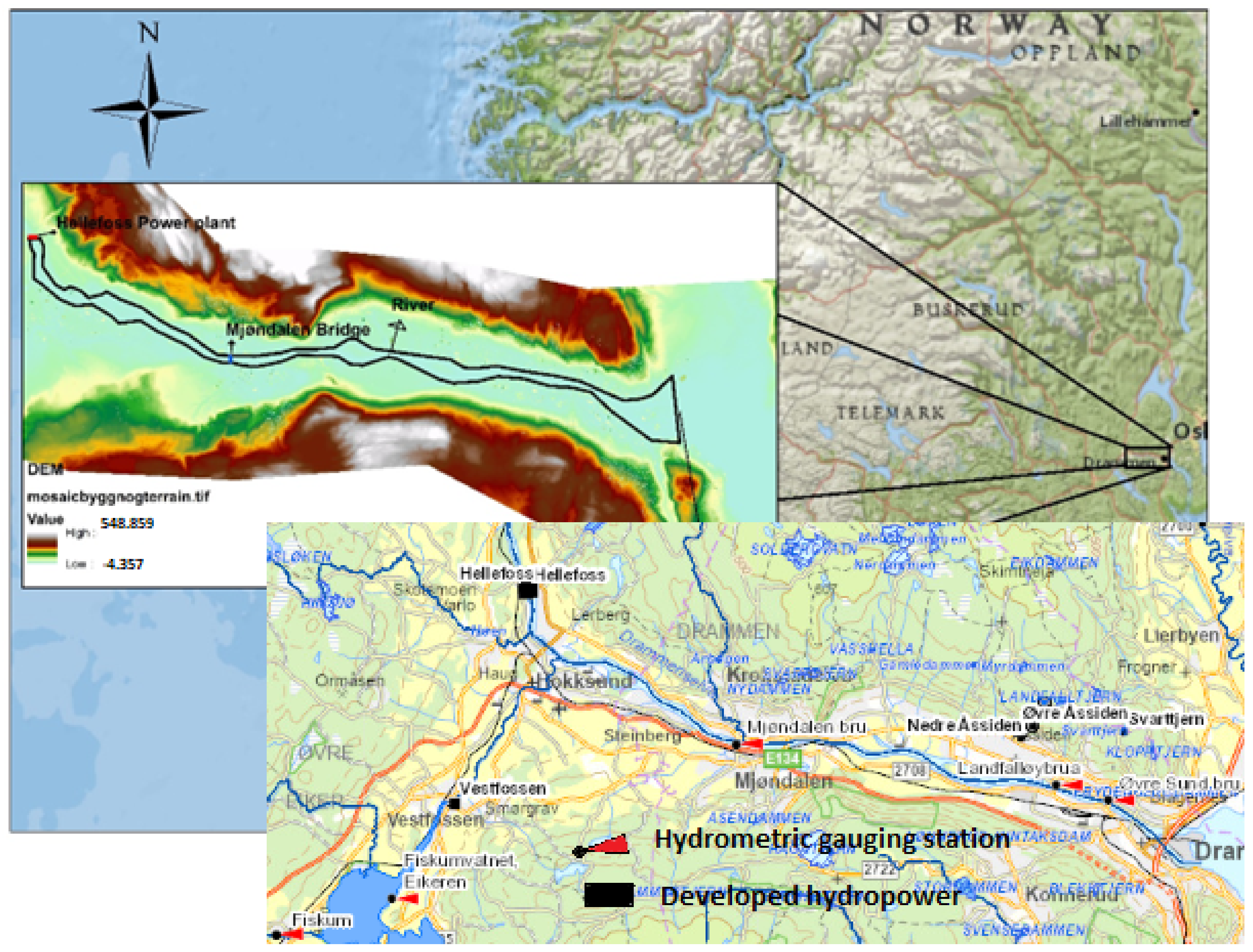
The study was conducted on the Drammenselva River, located in Buskerud County, southeastern Norway (see Figure 1). Drammenselva is one of the largest rivers in Norway, with a drainage basin of approximately 17,000 km2 and an annual average discharge of 300 m3/s. The river is 308 km long, which makes it the fifth longest river in Norway. The rainfall area is bounded in the north by Valdresflya and Jotunheimen, in the northwest by Filefjell and Tyin, in the west by Hardangervidda/Hardangerjøkulen and Numedalslågen’s catchment, and in the east by Gausdal, Nordmarka, Bærumsmarka, and Mjøsa’s catchment. The Drammens watercourse naturally divides into several sub-watercourses. The central river in the watercourse is the Drammenselva, which stretches 48 km from the Tyrifjord down to the outlet in the Drammensfjord. Three larger rivers join this stretch: Vestfosselva from Eikeren with a catchment area of 533 km2, Simoa from Eggedal and Sigdal with 887 km2, and Snarumselva (Hallingdalselva) with a catchment area of 5252 km2.
The river Drammen is wide and flows almost completely down towards the Drammensfjord. The Drammen River lies in a valley that varies in width, with narrower sections and wider sections. The riverbed between Hagaøya and Hokksund is just over 9 m deep and approximately 100 to 250 m wide. The area has a total length of approximately 3.2 km. The riverbed here is characterized by dune forms. The riverbed between Mjøndalen and Steinberg is up to 13.8 m deep and approximately 180 to 320 m wide. The area has a total length of approximately 4.6 km. The riverbed between Langesøya and Nedre Eiker is up to 14.5 m deep and between 80 and 500 m wide. The area has a total length of approximately 5.8 km. Langesøya divides the river in two and is approximately 1 km long and 250 m wide. The riverbed between Bragernes and Lillemoen is up to 14.5 m deep and between 100 and 400 m wide. The area has a total length of approximately 5.4 km. The hydraulic gradient between Hokksund and Mjøndalen is approximately 0.0006 m/m.
On its way to the sea, Drammen River passes a series of rapids and waterfalls. The largest are Vikerfoss, Geithusfoss, Kattfoss, Gravfoss, Embretsfoss, Døvikfoss, and Hellefoss. There are a number of power plants on the Drammen River, several with dams. The city of Drammen has spent substantial resources on developing attractive park areas along the riverside. There are around 39,000 buildings near the river Drammen, most of which are residential buildings. On the northern side of the Drammen River, the area between the city and the Holmen bridges in Drammen has also been developed, including the famous town square Bragernes Square (Bragernes Torg), the Tower Buildings, the Drammen Theatre (Drammens Teater), and Drammen Park. The port of Drammen is Norway’s largest port facility for cars. By the harbor there are industrial areas with a number of industries, including workshop, food and beverage, paper/stationery, chemical, and pharmaceutical industries. The stretch from Langesøya to the outlet in the Drammensfjord is characterized by urban development and some remaining industry. Large parts of the beach zone are heavily cultivated. The districts around the Drammen River are bound together by a dense road network and several bridges over the river Drammen. The Drammensbrua on the E18 is Norway’s longest bridge at 1892 m. Today Drammenselva is also used for recreational purposes and is known for its excellent Atlantic salmon fishing.
The Drammen area is characterized by the fact that a large glacier filled the valley about 10,000 years ago. There is a lot of igneous rock in its area, which means that there is a lot of solid rock with bad infiltration/drainage. Under the igneous rocks, Cambro-Silurian sedimentary rocks are exposed in a belt a little south of Drammensdalen. There is marine clay, sand, and gravel below approximately 200 m in Drammensdalen, as well as in the lower parts of Konnerud.
The study area starts from approx. 245 m downstream of Hellefoss power plant (Hokksund) to the outlet into the sea at Drammen harbor and covers Øvre Eiker, Nedre Eiker, and Drammen municipalities. The model area extends over approx. 21 km.
The water flow conditions in the Drammenselva have constantly changed over the years due to a continuous increase in new regulating reservoirs. The regulation of the larger lakes in the lower parts of the watercourse Randsfjorden, Tyrifjorden, Sperillen, Krøderen, and Soneren probably has the biggest impact on the water flow conditions in the Drammenselva. The regulations in the watercourse have led to an increase in the winter water flow and a dampening of the spring floods.
The largest floods in the Drammenselva in recent times occurred during the first 30 years of the 20th century when there were still relatively few regulated reservoirs in the watercourse. Most of them were spring floods that occurred in May and June. Some were autumn floods in September. The two largest floods, at the end of June 1927 and in mid-June 1926, had a daily average water flow of 2324 m3/s and 2197 m3/s, respectively, which shows that the flood in 1927 is estimated to be a 100-year flood, while the flood in 1926 had a recurrence interval of 50–100 years.
In recent years, there have been several floods in the watercourse, such as in 2007 when there was a flood with a recurrence interval of approximately 10–20 years. There was also a flood in September 2011 that was just over a medium flood and in May 2013 corresponding to a 5 to 10-year flood.
2.2. Data
2.2.1. Flood Hazard
A digital elevation model (DEM) of 1 m resolution for the study area was obtained from Høydedata “www.hoydedata.no (accessed on 12 February 2021)”. River cross-section data from Hellefoss power plant to the port of Drammen, which consists of 96 cross sections, was obtained from NVE. The geometry of the bridges is taken from measurements made by NVE. Table 1 shows all the properties used in the model for all bridges.
Annual maximum flow values for the present climate were estimated using frequency analysis for selected ARIs (average recurrence intervals). The frequency analyses and computation of flood magnitudes for different average recurrence intervals up to 1000 years was done by NVE and reported by Ejigu et al. [33]. The results of water flow simulation of a changed climate for the Drammenselva suggest that the 200-year floods in the Drammenselva will not increase until 2100 as a result of climate change [34]. For smaller tributaries with precipitation fields less than 100 km2, Lawrence [34] recommends assuming a 20% increase in flood water flows for the 200-year flood until the year 2100. The assessment of the increase in future floods is based on a comprehensive analysis using a combination of 10 different climate scenarios (based on GCM–RCM combinations from the CORDEX project [35]), two different downscaling methods, and 25 different realizations of a hydrological model set up for 115 reference catchments in Norway [34,36]. This gave a total of 500 simulation results for each of the catchments for two different emission scenarios (RCP 4.5 and RCP 8.5). Based on these simulations, flood frequency analysis was undertaken for the historical and future periods, and percentiles from the resulting flood distributions were used to compute the percentage of increase in the design floods. The analysis led to a set of spatially varying growth factors for future floods (1.0, 1.20, and 1.40), which forms the basis for future design flood analysis in Norway [34]. Since this is a comprehensive study of Norwegian floods and this is the method recommended for practical applications, we have opted to use this method for the analysis in Drammenselva. The resulting flood values in the Drammenselva will then be as given in Table 2, which was then used as flood mapping input data in the HEC-RAS model.
Water flow during floods in the Drammen River is provided for the tributaries or local catchments. This water flow is less than during floods in the individual local fields. Extreme water levels at sea for different repetition intervals are calculated by the Norwegian Mapping Authority, the sea division, and the result is taken from NVE’s flood zone map report. Table 3 shows storm surge water levels for different return periods under present and future climates.
The observed water levels and calculated discharge data from the 2007 and 2013 flood events have been provided by NVE for the calibration and validation of the flood model.
2.2.2. Land-Use Information
Land use was analyzed on the basis of two main elements, namely, buildings and infrastructure (roads and rail roads). The land-use polygon layer was downloaded from the Norwegian Mapping Authority’s portal Geonorge “www.geonorge.no (25 February 2021)”.
2.2.3. Vulnerability Factor (Depth–Damage Curves)
Since there were no site-specific curves in the studied area, depth–damage curves developed for NVE’s cost–benefit analysis tool were considered for this study. These curves were created for different types of land use using what-if analysis and flood expertise acquired from past flood events. This tool has been developed using 16 different categories of buildings and seven categories of infrastructure based on the main land uses identified in Norway. The land-use data sets also include basements. Therefore, like the properties on the ground floor, the basement blocks will have a surface assigned to each land-use class. Consequently, it is related to depth–damage curves that do not depend on the ground-floor uses. The damage in the basement is determined using negative depths. In these approaches, the water fills the basement first, and then it reaches the ground level (depth–damage relationships for all land-use types are provided in the Supplementary Material).
2.3. Development of Flood Hazard Modeling
The flood hazard was determined using the hydraulic simulation of flooding. The assessment process involved the collection and preparation of geometric data, hydraulic modeling, and GIS post-processing and mapping.
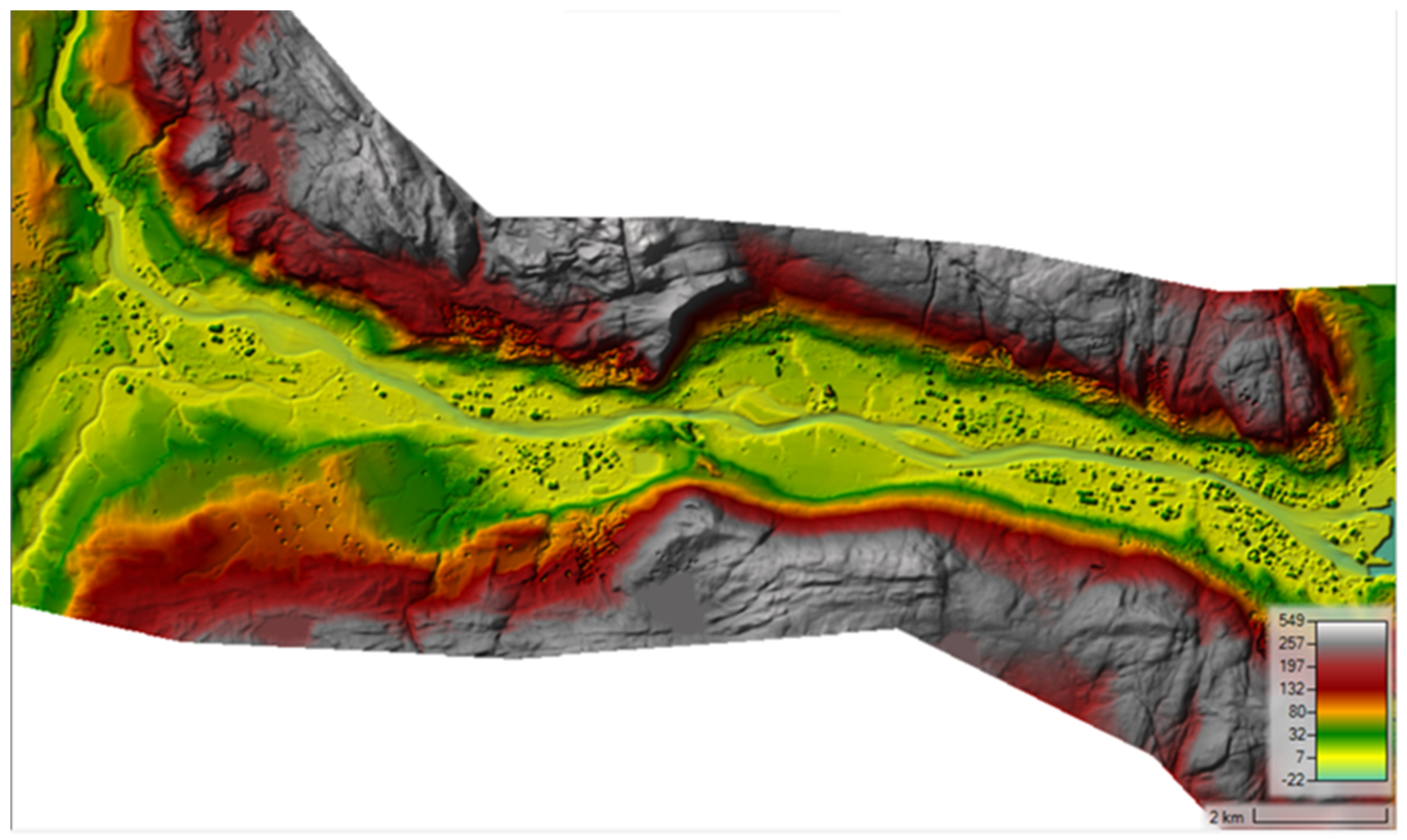
The DEM represents land-elevation data, which is essential for estimating the storage volume of surface flooding. As a result, the output quality is determined by the DEM quality. The DEM was collected using topographic (red) lidar, which does not contain the bathymetry of a river channel. The terrain model was therefore integrated with the bathymetry data by combining a set of cross sections collected by NVE for an earlier flood zone mapping project [33] with the DEM. The 1D geometry was imported into HEC-RAS, in the standard geometry editor the bank station location in the cross sections was manually edited to match the DEM. The elevation data of the areas in between the cross-sections was then interpolated into an elevation model, and the new geometry was exported as a raster. The final step was to merge the bathymetry model with the topographic DEM in HEC-RAS Ras Mapper to form a combined digital model for the study area with a resolution of 0.35 × 0.35 m. Buildings have also been represented in the model by extracting the land occupied by the buildings from the DTM using building information from the Norwegian Mapping Authority and then raising each building by 3 m in the DEM to make it an obstacle for the water flow in HEC-RAS flood simulations. HEC-RAS version 6 beta 3, the latest version at the time of this study, hydraulic modeling software was used in this project, which was developed for the analysis of 1D steady flow and 1D and 2D unsteady flow. The 2D model simulates water flow in both longitudinal and lateral directions on terrain represented by a finite mesh continuous surface. The finite mesh allows for continuous interaction between the main river and the floodplain, allowing the 2D model to accurately represent velocity and water depth variations over the floodplain. Therefore, the use of the 2D model becomes essential for the accurate estimation of the flood-depth grid. The 2D model can be expected to work well in the rivers with wide and flat floodplains, where the flow goes out into the overbank area. For a micro-scale assessment such as this, a highly accurate estimation of flood depth is critical. As a result, 2D approach was required in the model. The output of this model will be in the raster format in the depth grid, which can be imported into GIS for further analysis.
A 2D model was then set up in HEC-RAS v.6 beta using the combined raster (Figure 2). A 5 × 5 m (1.73 million cells) unstructured 2D computational mesh was created. The underlying 0.35 × 0.35 m terrain remained the computational basis for all depth, velocity, and inundation simulations. The model domain included the main Drammenselva River and four major tributaries: Hellefoss, Honselva, Vestfosselva, and the local catchment Mjøndalen bru, where the catchment drains into the sea at Drammen harbor. In addition, six bridges were included in the model. Even if some of the bridges have a curved shape, the lower and upper edges are defined horizontally in the model.
The bridges on the section between Hellefoss power plant and Drammen harbor are modeled in the 2D model using the “energy equation” method. This method is relatively easy to use and is well suited for the flow situation in the Drammen River which is subcritical. An example of how bridges are implemented is shown in Figure S1 in the Supplementary Material for the Mjøndalen bridge.
Boundary conditions were defined using the information from the frequency analysis in the NVE flood zone report [33]. The downstream boundary condition is defined by a stage hydrograph in the fjord with the highest average tide of a 10-year storm surge. In addition, the model domain was extended farther down in the Drammenfsjord to avoid any problems related to the boundary definition causing an impact on the results in the study area. The unsteady flow water surface computation was initiated at the upstream boundary using discharges with different return periods.
It can be complicated to develop a stable unsteady flow model for the computational domain. Model stability problems occurred initially during the simulation of Drammen River. Therefore, several sensitivity tests were conducted to improve the model’s stability and produce satisfactory results.
2.3.1. Model Calibration and Validation
To calibrate the model, observed sea water levels during the 2007 flood at the port of Drammen have been used as the lower limit condition, and calculated water flow for the main river and its major tributaries has been used as the upper boundary. The scaling method was used to calculate water flow for the main river and its major tributaries based on observed water flow data from measuring stations Mjøndalen bridge and Fiskum. The calculation of scaling was performed by NVE and reported by Bakkan & Øydvin [38]. The water levels from the flood from 6 July 2007, at 20:06 to 7 July 2007 at 00:22, which were registered at a number of places on the stretch between Hellefoss power plant and the port of Drammen, were used in the calibration. This return period of flood corresponds approximately to 10 years. In addition, a water level measurement made on 24 May 2013, at Mjøndalen bridge was used for the validation. The land-use distribution was obtained from the Norwegian Mapping Authority (Kartverket), and different Manning values have been assigned according to the literature [39]. By comparing observed and simulated water surface levels at multiple locations, the model parameters were adjusted. The roughness coefficient was adjusted to fit the simulation results to the observations through a trial-and-error procedure. For different land-use classes, a range of roughness coefficients were tested. The built-up areas (0.02) and open fields (0.03) were assigned the lowest values of Manning roughness coefficients. On the other hand, forests (0.15) and marsh areas (0.30) were assigned the highest roughness value. The inundation modeling simulation time was 5 h, which accounted for the 5h maximum water flows of the 2007 flood, and the output time step was 5 s.
Evaluation Criteria for HEC-RAS Models
The coefficient of determination (R2) and root mean square error (RMSE) were used to evaluate the agreement between the modeled and observed values:
where = ith value in observed values; = ith value of modeled data; and m = number of total observations.
2.3.2. Flood Hazard Determination
The flood hazard modeling process allows for the acquisition of a broad set of primary hazard indicators, which alone gives good insight into the potential magnitude of a flood event in the study area. The raster of water depth (d) and flow velocity (v) for each flood scenario (Q100, Q200, Q500, and Q1000) were used as input data for the computation of flood intensity (FI) using Equation (1).
The flood intensity for each scenario was used to define the flood hazard in the model area. The flood hazard is assumed to be higher if the flood intensity is higher. Hazard classifications were developed based on the works of Beffa et al. [40], which were used to develop hazard classifications. According to Beffa’s work, flood intensity is considered as FI > 2 for high hazard, 0.50 < FI ≤ 2 for medium hazard, and FI < 0.50 for low hazard.
2.4. Flood Damage Estimation
This impact assessment will consider direct and some indirect tangible damages at a micro-scale level by using depth–damage curves. Flood damage assessment requires the integration of the physical impact results (flood depth) with information on exposure and vulnerability or impact. Direct damage estimates were obtained by intersecting land-use data with flood depth data and extracting the exposed objects by the means of a GIS. The exposed objects were then integrated with the corresponding depth–damage functions and unit cost in the damage estimation model. This resulted in the estimation of damage for each of the return periods considered (100, 200, 500, and 1000 years), which allows for the evaluation of the change in flood damage between the current and future climate for the respective return periods. To ease the calculation of the final flood damage estimation, an Excel-based toolbox from NVE [32] has been used. This toolbox enables the user to increase the speed of the post-processing of data and ease the simulation of several events. The following equation illustrates how the elements in the direct damage model are combined to estimate the total amount of physical damage in a flooded area:
- Dmax,i: maximum damage for land-use category i;
- i: land-use category;
- r: location in flooded area;
- m: number of damage categories;
- n: number of locations in flooded area;
- αi(hr): stagedamage function for category i as a function of flood characteristics at a particular location r (0 ≤ αi(hr) ≤ 1); and
- ni,r: number of objects of damage category i at location r.
Flood Cost Estimation Model
The tool was developed on behalf of and in cooperation with the Landslide and Watercourse Department in NVE by Nils Roar Sælthun in 2015 [32]. The tool was originally a cost–benefit analysis tool that was built into a Microsoft Excel spreadsheet. However, only the flood damage portion of the tool was used in this study. The tool was made in accordance with the Norwegian Directorate for Financial Management’s guidelines. The tool provides basic data for municipalities and fixed model constants, which are not usually changed during operation. The fixed data defines default values, discount rate, expected GDP development, and vulnerability factors. The default values are largely based on data from Statistics Norway and are adjusted on the basis of the construction cost index and the consumer price index.
Direct and some indirect tangible costs are handled in the damage tool. Therefore, the total flood damage consists of the damage to buildings, agricultural areas, infrastructure, and other costs. Other costs include fracture repair, cleanup and rental costs, mobilization, and other first-line costs. These are explained below.
Fracture cost of roads: These are breakage costs for roads are based on detour costs when closing, based on an estimate of costs per extra km driven.
Cleanup and rental costs: These are costs related to cleaning up in the event of total damage, and rental costs in the renovation and construction period. No input is required. It is assumed that all homes where there has been water on the ground floor will need renovation or new construction.
Mobilization and other first-line costs: These are societal costs associated with handling the actual incident, with a fixed estimate of 5% of material damage.
For this study, the damages to buildings, infrastructures, and other costs, excluding fracture cost of roads (due to unavailability of data), were considered for the damage estimation of the study area.
There are different parameters in the tool that describe the time of development. The parameters used in the flood cost estimation tool are price indices and welfare development. An important point is that present value is used for flood cost estimation, and that future price increases are not taken into account.
Price indices: The tool largely operates with standard prices for replacement values, taken from surveys by Statistics Norway and others, as a basis for the utility calculations. If these are fixed in the tool, as time goes on and the price increases significantly, the costs will increase while the utility values are fixed. To avoid this, Statistics Norway’s construction cost index and consumer price index are used to raise the standard values in the tool. VSL (Value of a Statistical Life) is also adjusted, from 2012 to the current year according to the CPI (Consumer Price Index). This therefore applies from the base year to the current year, not further into the future.
Welfare increase: The value of statistical life is largely based on society’s willingness to pay. There is a clear connection between the level of welfare, expressed by gross national product per capita, and the willingness to pay to save lives. In accordance with the Directorate for Financial Management’s “Guide to Socio-economic Analysis”, VSL has therefore been adjusted upwards through the planning horizon in accordance with expected real growth in GDP per capita. In the government’s perspective report from 2013, this was estimated at 1.3% per annum for the period of 2012–2060. In practice, this comes as a reduction in the discount rate for VSL, so that the present value of life saved in the future falls less with time than material values. The Excel-based flood cost estimation tool is included in the Supplementary Material.
3. Results
3.1. Model Calibration and Validation
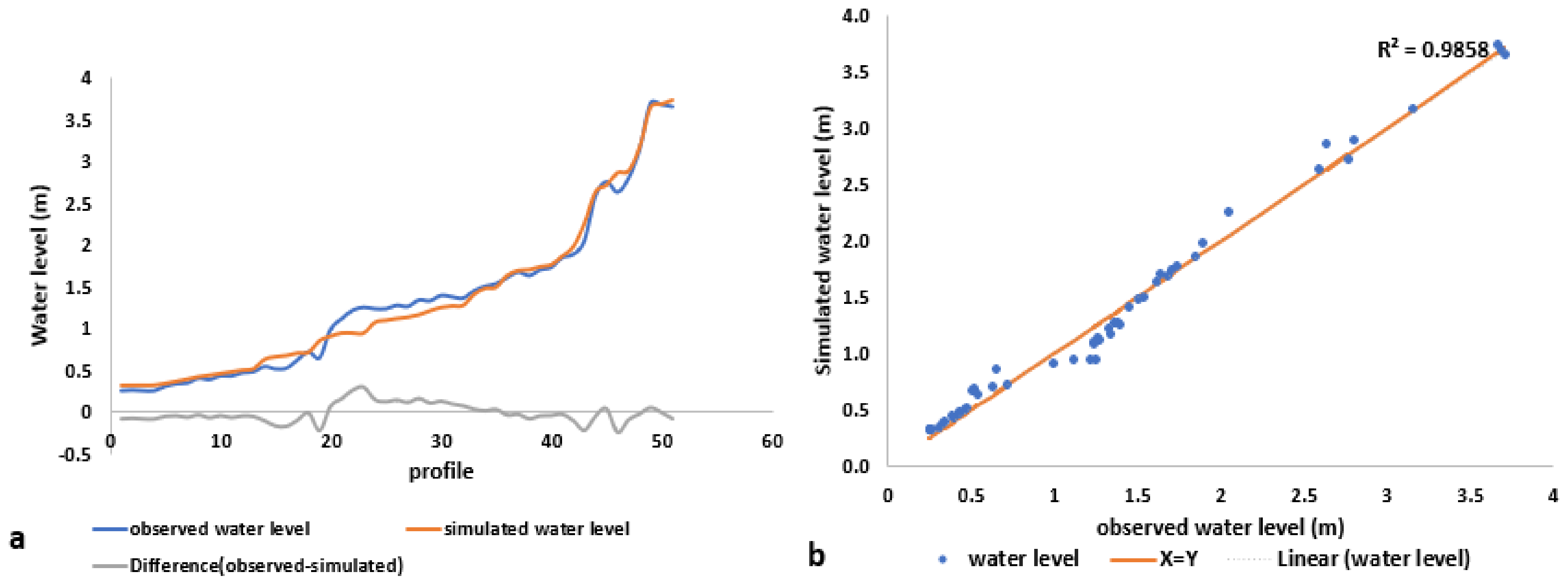
The flood model did not give a satisfactory result in the first run. As a result, the flood model must be calibrated for the desired results. Figure 3 shows the simulated water surface elevation and the water level of the surveyed flood after calibration. In general, it can be said that the simulated results are close to the actual situation when compared to the surveyed flood. The statistical indicators computed for the observed and simulated model outputs were good (R2 = 0.99 and RMSE = 0.11 m) (Figure 3b). The validation result also shows that there is a good agreement between observed and simulated water levels; see also the last column to the right in Table 4.
3.2. Flood Hazard Modelling
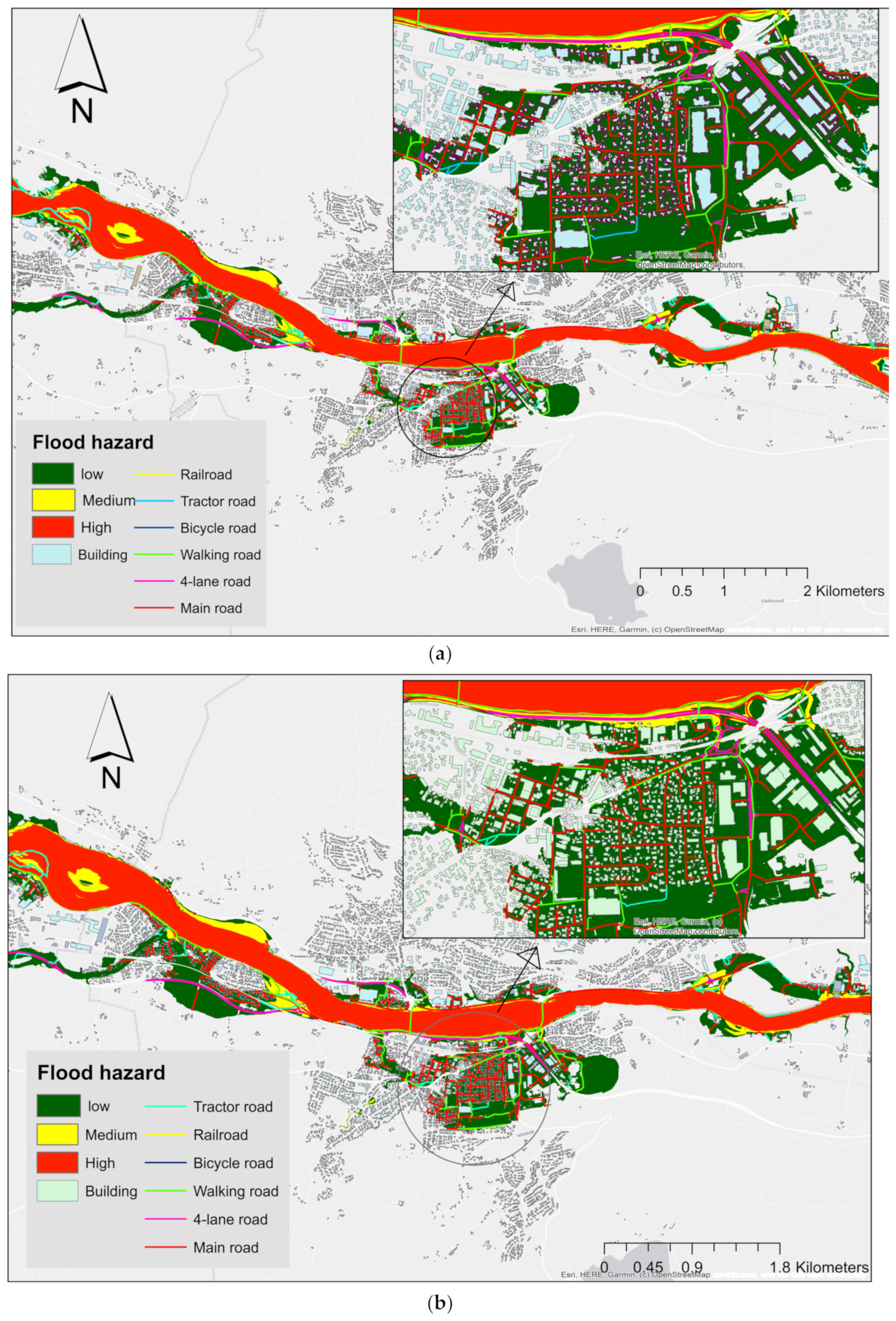
This section focuses on four hazard indicators: flood intensity, flood extent, velocity, and water depth. Flood hazard maps in Figure 4 show areas with their corresponding hazard categories and flooded buildings and infrastructure for both current and future flood scenarios. Flood hazard is mostly low or medium, while high flood hazard occurs in the stream channels, with the exception of some other minor inundations in the current (5.87 km2) and future (5.96 km2) climates.
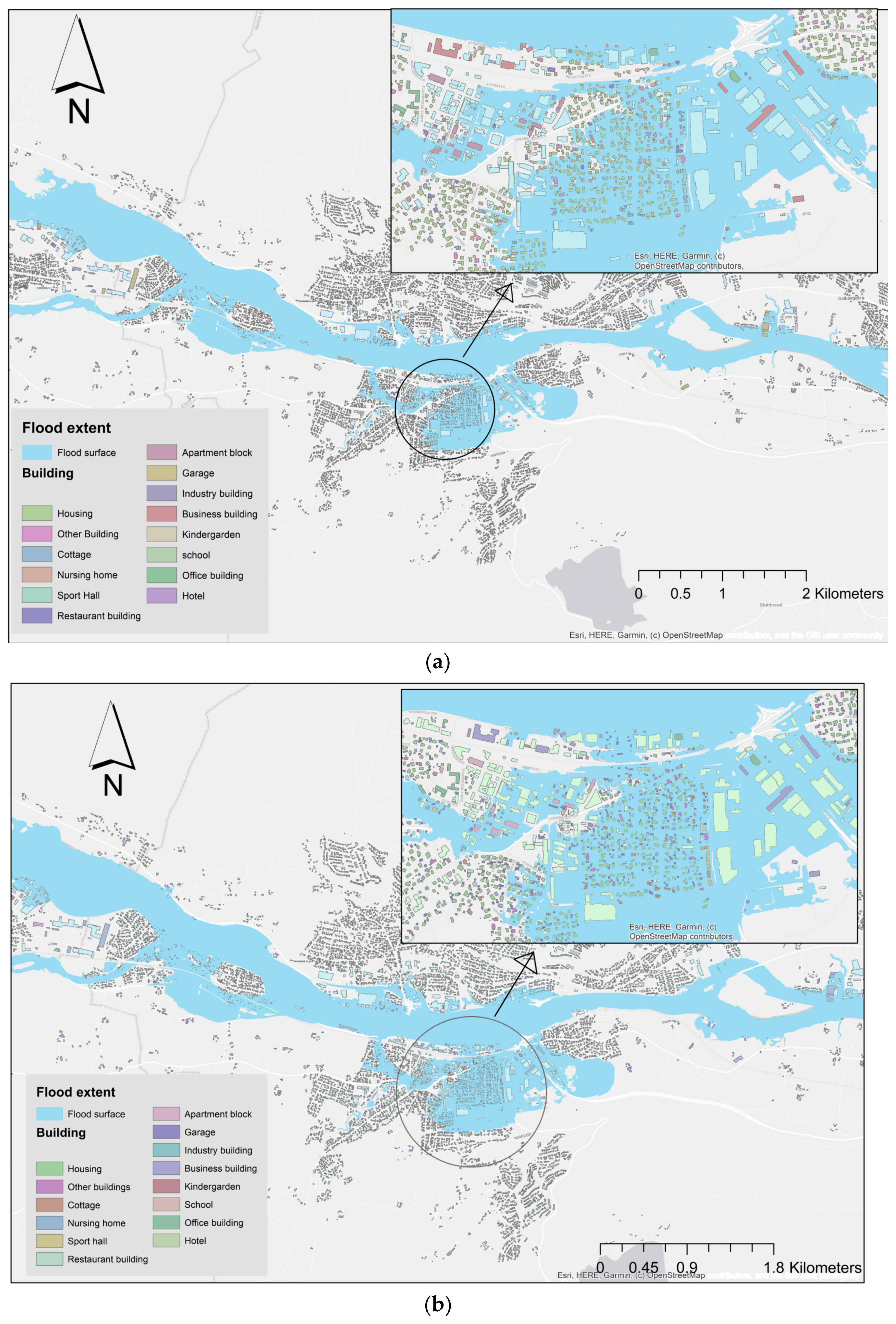
As for the flood extent in Figure 5, it was found that for both the current and future 200-year climate scenarios, the study area was significantly affected by the flood scenario. As illustrated in Figure 5, 2399 and 2855 out of the 39,000 buildings considered in this analysis are potentially affected by current and future climate 200-year flood scenarios, respectively.
In absolute numbers, about 68,813 m2 and 81,348 m2 of a total of about 6,292,039 m2 of built-up area are affected by the 200-year flood scenario of the current climate scenario and future climate scenario, respectively. This shows that the future climate scenario corresponds to approximately 18% higher than the current climate flood.
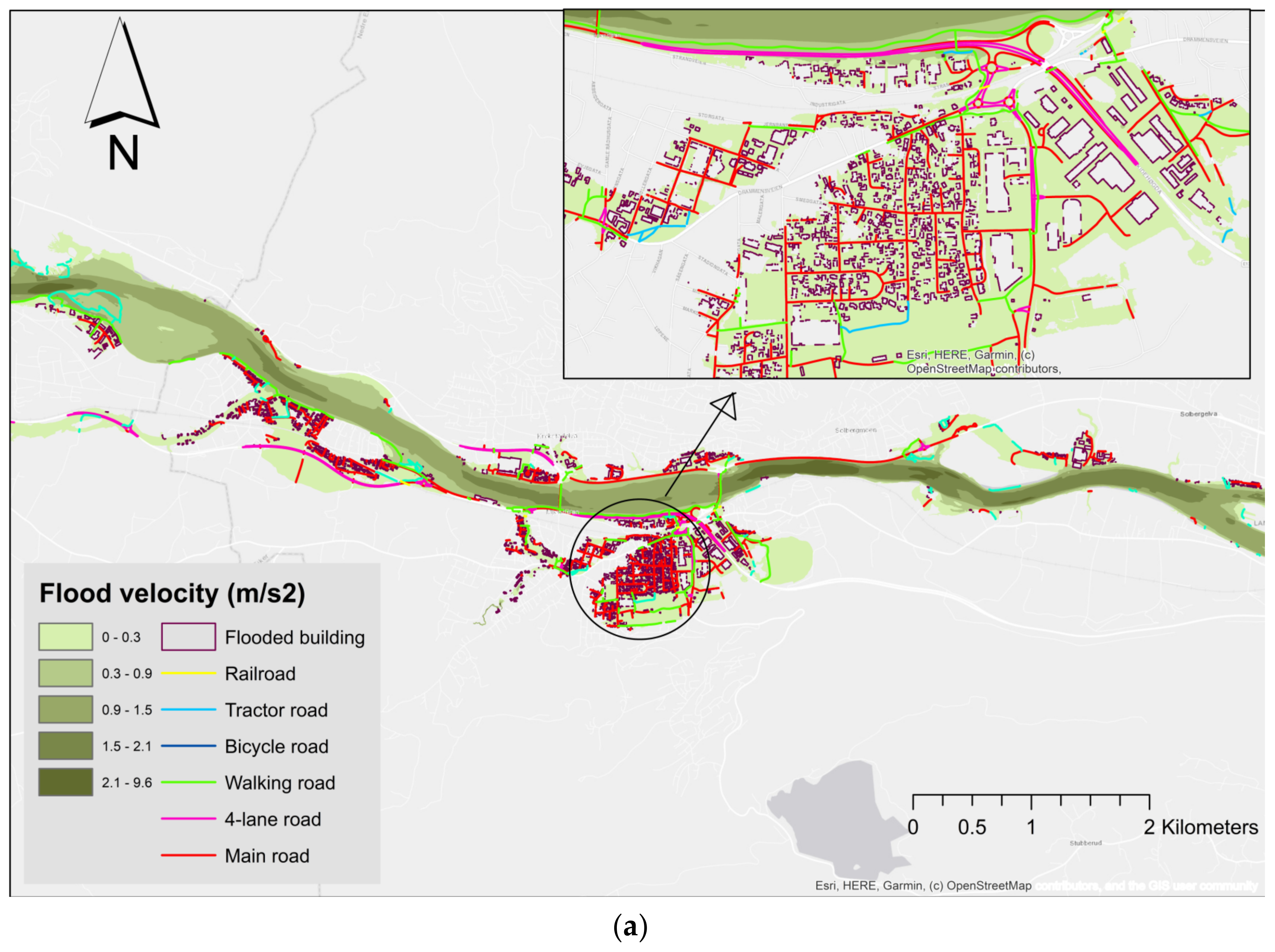
Concerning the flood velocity (Figure 6), it ranges between 0 m/s and 9.62 m/s for the current 200-year flood scenario and between 0 m/s and 10.33 m/s for the future climate flood scenario. The average velocity value at the surface of the 2399 buildings affected by the current climate flood is about 0.26 m/s, with a standard deviation value (STD) of 0.07, being that 25 of these 2399 buildings are exposed to surface velocities higher than 0.50 m/s. The mean velocity value at the surface of 2855 buildings affected by the future climate flood is 0.26 m/s with a standard deviation value (STD) of 0.13. Of these, 27 out of the 2855 buildings are exposed to a surface velocity higher than 0.50 m/s.
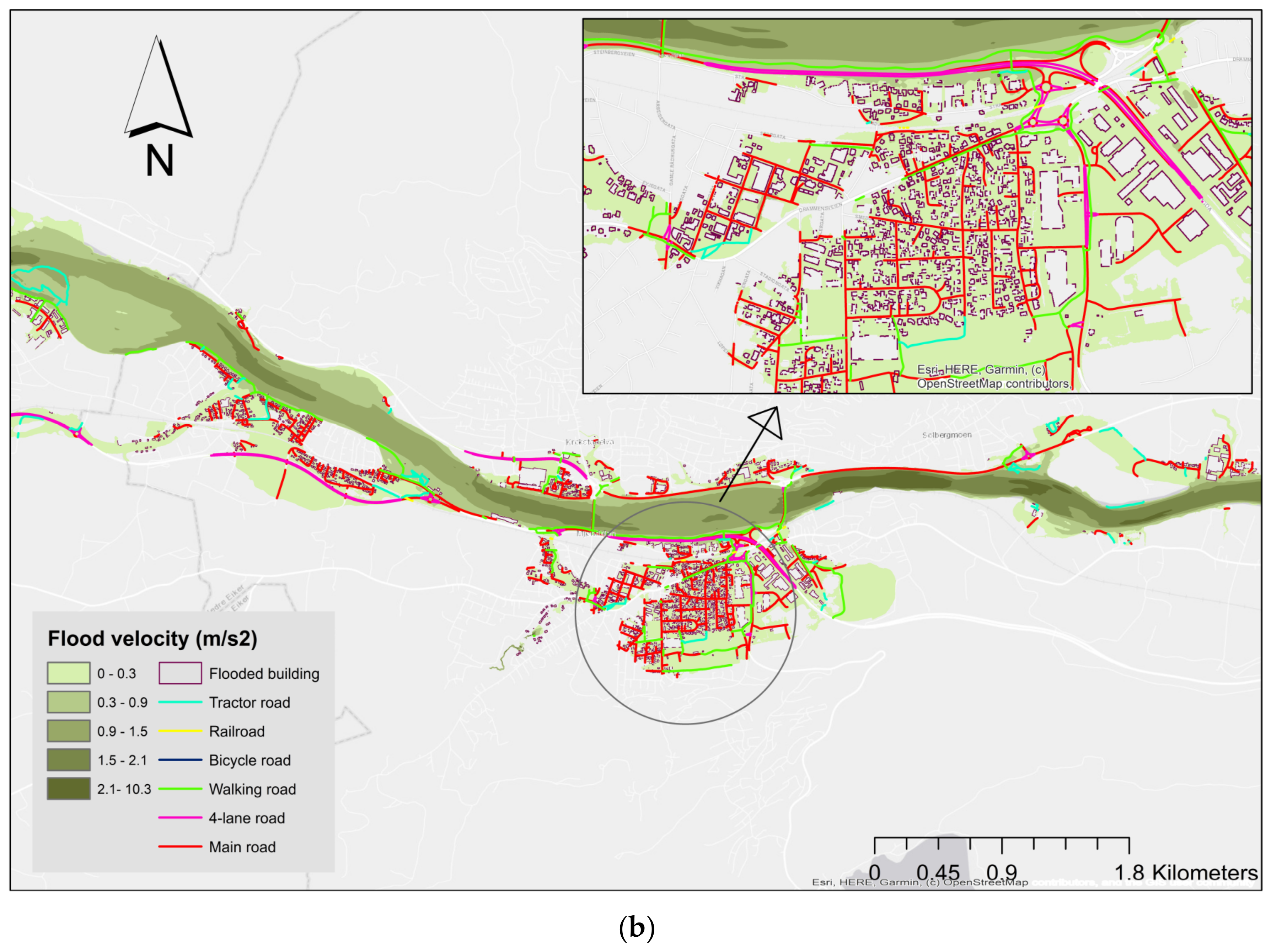
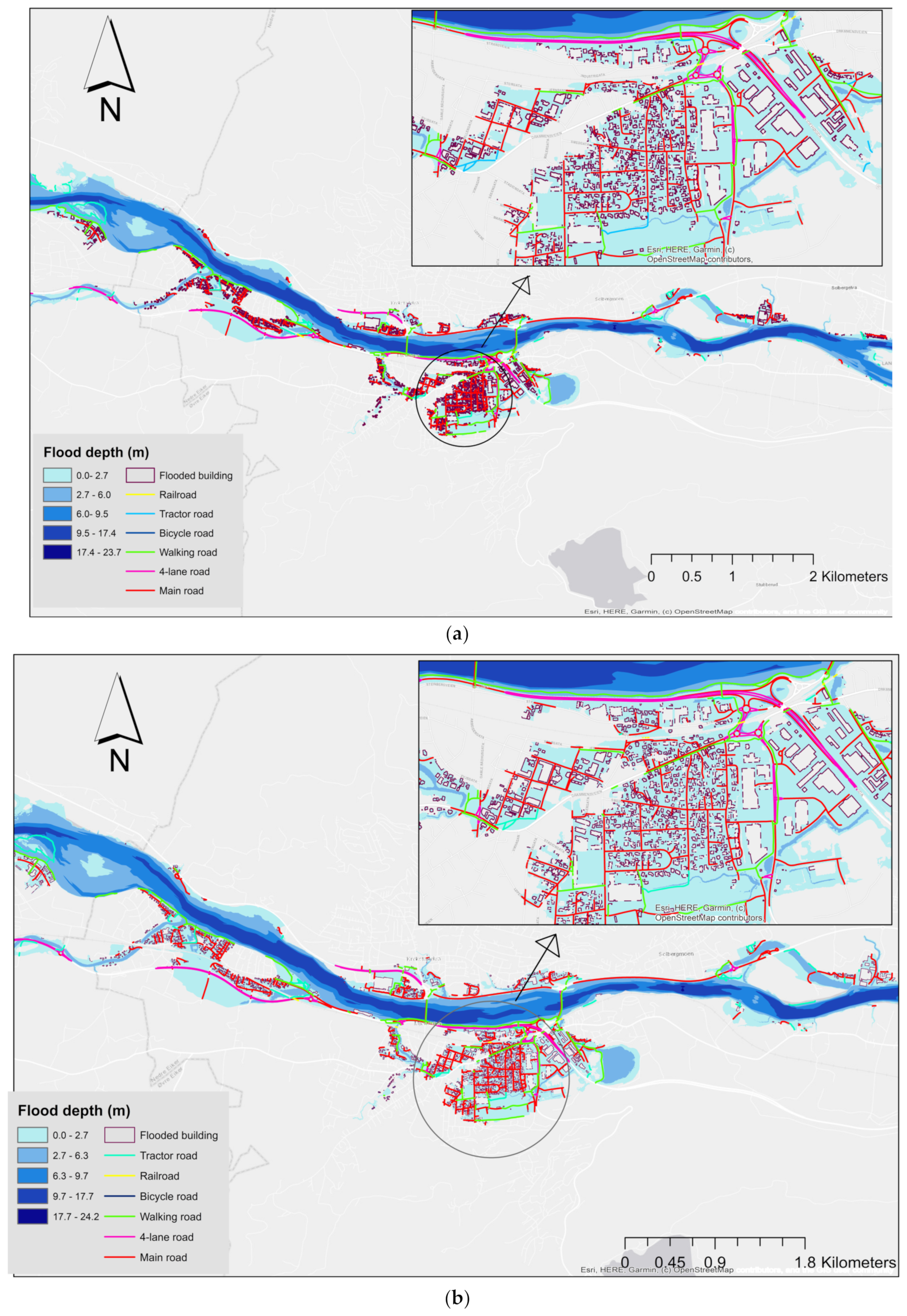
As for the water depth in Figure 7, from the hazard analysis, it was found that for the considered current and future climate scenario of 200-year flood, the buildings will expectedly be exposed to an average depth of about 0.72 m (SD = 1.20) in the current climate flood and 0.73 m (SD = 1.18) in the future climate flood. As illustrated in Figure 7, 795 out of the 2399 buildings were affected by a water height of more than 0.5 m in the current climate flood. About 1093 out of 2872 buildings affected by a water depth of more than 0.5 m in the future climate flood correspond to the affected building in the future being approximately 37% higher than the current flood-affected building.
Table 5 summarizes the above-discussed results, presenting the absolute and relative number of potentially affected buildings for different ranges of flood velocity and water depth.
As presented in Figure 4, Figure 5, Figure 6 and Figure 7, it was found that about 85,658 m and 110,037 m of infrastructure (roads and railroads) were affected by the current and future climate of a 200-year flood scenario.
To conclude, the comparison between the current and future scenarios in 2100 showed that the inundated areas, velocity, and depth increased, as presented in the flood hazard modelling section. Detailed flood hazard maps of different flood scenarios (Q100, Q500, and Q1000) are presented in the Supplementary Material (Figures S2–S13). Furthermore, the affected number of buildings and length of infrastructure (roads and railways) for each flood scenario are tabulated in the Supplementary Material (Table S1).
3.3. Flood Damage
The total expected flood damage is computed in Mill.kr over the land-use categories for which depth–damage functions were derived. Table 6 gives the estimated breakdown of damage under every flood scenario for the area under study. It is observed that the cost of flood damage to a building (structural plus content) covers about 90–92% of the total cost estimated over all land-use categories under each flood scenario. Furthermore, the damage cost in Table 6 verifies the fact that the smaller the exceedance probability gets, the higher the expected flood damage becomes. The results also show that the impacts of climate change increase the vulnerability of urban areas to flooding and economic damage, which will increase the total damage from floods by 20.26%.
4. Discussions
Flood cost estimation is a combination of flood hazard, vulnerability, and exposure. This study shows that flood damage is mostly affected by the hazard component, i.e., flood depth. The average velocity value at the surface of the buildings in the flood-prone area affected by the current and future climate floods is about 0.26 m/s, which has a minor effect compared to food depth. Therefore, the study uses locally developed depth–damage functions for the above-mentioned land-use groups with the aim of contributing to the development of a standard approach for estimating expected flood damage. As for building damage, the area of housing properties is larger than the other building categories considered (see Table 7). This generates a higher number of flood-affected properties in each flood scenario. As a result, the total estimated damage (structural plus content) to housing is higher than other building categories. As for the 1000-year flood for the current climate flood, the total estimated damage for housing is approximately 360.58 mill.kr, which is higher than other building categories. The second most highly affected building category is industrial buildings, which are estimated at approximately 225.75 mill. kr. Moreover, it is observed that the cost of flood damage to buildings (structural plus content) covers about 90–92% of the total cost estimated over all land-use categories under each flood scenario.
The effects of varying ARI on flood damage in Table 6 verify that as the return period used to estimate the risk increases, the flood damage will also increase, but as the return period decreases, the total damage will reduce. Moreover, it is noted that for the 1000-year current climate flood, the total damage is 1127.40 mill.kr, about 48 % higher than the damage for a 200-year flood (784.31 mill.kr) and is approximately 18.40 % higher compared to the risk of a 500-year flood (952.31 mill.kr). This result corroborates the findings of [22,41,42], who found similar trends in their probability–damage relationships, with low probability events contributing to large damage values. Ward et al. [42] show how the annual flood risk estimate increases as the maximum return period used to estimate that risk increases. The study identified that the curve flattens off rather abruptly at return periods between 1000 and 2000 years, and there is a steep increase for low values of the maximum return period used. Olsen et al. [22] compared the results of calculating the EAD (expected annual damage) with three different methods. The results show that the three approaches provide remarkably comparable outcomes. For both the Olsen et al. [22] and Velasco et al. [41] case studies, a log-linear relationship was observed in the damage–probability curves. However, they also discovered a shift in the curves, with smaller events following one log-linear connection and larger events following another.
The findings reveal that climate change’s impact on flood risk makes urban areas more vulnerable to floods and economic loss. The effect of climate change will raise the total damage from floods by 20.26 %, according to the findings. This result is similar to that of Arnell et al. [11], who used climate models and socio-economic data to evaluate the future scenario of flood risk.
General Limitations
Regarding the results and methods used, possible sources of uncertainty and improvements should be considered and discussed. When applying the framework outlined in the methodology section for micro-scale flood damage assessment, it was necessary to adopt the following assumptions, which should be kept in mind when interpreting the results.
The climate data used for the projection of future floods are uncertain, which may have a considerable influence on the flood return level estimates. Therefore, this may lead to the uncertainty of future flood damage cost.
The approach is based on direct and some indirect flood damage caused by different water depths on different land-use typologies. Other factors that could lead to an increase in losses, such as flood velocity, building characteristics, sediment content in water, and some indirect economic losses, are not considered in this study.
Due to the absence of reasonable micro-scale land-use change data for the future climate, changes in land use and land cover are not integrated into the economic impact evaluation. Hence, it only reflects the influence of climate change on flood risk, which may lead to an underestimation of future flood risk.
It is normally assumed that a damaged object will have the same quality level after a repair as it had before the flood occurred. For some objects, such as buildings, it may happen that the repair leads to an increase in value in relation to the previous condition, due to the fact that the price is independent of the building’s condition before the flood occurred. Despite the fact that this contradicts typical perceptions of what damage is, it has not been possible within the scope of this study to exclude compensation that increases the value.
As for damage estimation applied, all the buildings affected by the flood have a basement, and all of the building categories are made from metal and concrete except housing (made of timber). The assumptions made for the infrastructure data include that 50% of private roads are made from gravel and 50% are made from asphalt, while the other road categories such as municipality, county, and highway roads are made up of 100% asphalt. All these assumptions may lead to the uncertainty of the estimated flood damage.
Due to the lack of and incomplete historical damage data, previous flood risk assessment studies found it difficult to validate flood damage estimates. This study also faced the same challenge. Flood damage estimation was undertaken for buildings and infrastructure. However, due to a lack of surveyed data, verification of the results with actual surveyed data was impossible.
As a final remark, despite the advances in data assessment and model development, there is still room for future research and improvement. Applying advanced statistical methods could help to elaborate in detail on the complex interactions of damage influences in general and the connection between flood probability and damage-generating parameters in particular. Empirically derived loss models usually suffer from a lack of information about damages caused by infrequent extreme events and hence are not very accurate in estimating the impact of such events. As it is the case in our data set, a uniform loss function has been applied to low probability and high probability flood events, and the loss estimation only focuses on flood impact variables such as flood depth. This data gap could be closed by establishing a framework for continuously assessing flood losses and thereby creating an up-to-date data set that describes flood damage representatively.
5. Conclusions
This article describes which contemporary methods exist and how they might be implemented in practice. The finding of the performed scoping study demonstrate which elements must be taken into account in contemporary GIS-based assessments of current and future flood damages. The utility of the findings may be seen in the universality of the proposed methods to assess flood hazards and flood risks, which could be used by practitioners in flood risk management to develop suitable assessment approaches to estimate flood damages for current and future scenarios. Flooding scenarios presented herein combine climate change–induced river flooding with other coastal flooding (storm surges) triggers to map flood risk. These maps can be considered an effective tool for risk reduction. It supports decision-makers in taking suitable actions under different risk conditions, particularly in the pessimistic scenario, where the highest level of flood hazard occurs. The quantitative result of the case study suggesting an increase of flood damages along the Drammen River in the future. The extreme flood risk largely occurs in the stream channels, with the exception of some other minor inundations. The evaluation result shows that 17% and 16% of the area is above medium risk under the current and future climates, respectively. The recurrence interval and the loss extent were shown to have a highly significant positive correlation. The assessment of flood hazards shows that the risk to buildings will be more serious in the future. Climate change and increased urbanization may have an impact on the degree of flood hazard and loss. Nevertheless, flood mitigation measures such as lake preservation and WSUD (water-sensitive urban design) implementation may help reduce flood impacts. Additionally, the detection of priority areas for flood risk reduction using flood hazard maps will be helpful to decision-makers as they adopt strategies at local and regional scales. The research results can provide valuable information for urban flood risk management and flood mitigation planning in the study area and other regions with similar conditions.
Supplementary Materials
The following are available online at https://www.mdpi.com/article/10.3390/w15050920/s1, Figure S1: definition of Mjøndalen bridge in the model, Figure S2: Flood intensity in the model area for the 100-year flood scenario under current climate, Figure S3: Water depth resulted from 100-year flood under current climate, Figure S4: Flood inundation map of 100-year lood under current climate. the colours in the above figures show different types of buildings and flooded surface in the study area, Figure S5: Flood velocities resulted from 100-year flood under current climate, Figure S6: Flood intensity in the model area for the 500-year flood scenario under current climate, Figure S7: Water depth resulted from 500-year flood under current climate, Figure S8: Flood inundation map of 500-year lood under current climate. the colours in the above figures show different types of buildings and flooded surface in the study area, Figure S9: Flood velocities resulted from 500-year flood under current climate, Figure S10: Flood intensity in the model area for the 1000-year flood scenario under current climate, Figure S11: Water depth resulted from 1000-year flood under current climate, Figure S12: Flood inundation map of 1000-year lood under current climate. the colours in the above figures show different types of buildings and flooded surface in the study area, Figure S13: Flood velocities resulted from 1000-year flood under current climate, Table S1: The number of flood-affected buildings at various recurrence intervals, Table S2: length of flood-affected infrastructure at various recurrence intervals in meters. An excel-based flood cost estimation tool that includes the depth damage relationships is provided as an excel file.
Author Contributions
Conceptualization, S.F.H. and K.A.; Data curation, S.F.H. and K.A.; Formal analysis, S.F.H. and K.A.; Methodology, S.F.H. and K.A.; Resources, K.A.; Software, S.F.H.; Supervision, K.A.; Validation, S.F.H.; Writing—original draft, S.F.H.; Writing—review and editing, K.A. All authors have read and agreed to the published version of the manuscript.
Funding
S.F.H. is funded by the NORAD scholarship as part of the Hydropower Development Master’s Program.
Institutional Review Board Statement
Not applicable.
Informed Consent Statement
Not applicable.
Data Availability Statement
The authors confirm that the data supporting the findings of the study are available with in the article and its Supplementary Material. Raw data that support the findings of this study are available from the corresponding author, upon reasonable request.
Acknowledgments
The authors wish to thank Péter Borsányi and Demissew Kebede Ejigu at NVE for providing the cross-sectional data and for providing information on previous work in Drammenselva. DEM and map data are provided by the Norwegian Mapping Authority—Geovekst and local communities.
Conflicts of Interest
The authors report there are no competing interests to declare.
References
- McGrath, H.; Kotsollaris, M.; Stefanakis, E.; Nastev, M. Flood damage calculations via a RESTful API. Int. J. Disaster Risk Reduct. 2019, 35, 101071. [Google Scholar] [CrossRef]
- Romali, N.S.; Yusop, Z. Flood damage and risk assessment for urban area in Malaysia. Hydrol. Res. 2021, 52, 142–159. [Google Scholar] [CrossRef]
- Zeleňáková, M.; Fijko, R.; Labant, S.; Weiss, E.; Markovič, G.; Weiss, R. Flood risk modelling of the Slatvinec stream in Kružlov village, Slovakia. J. Clean. Prod. 2019, 212, 109–118. [Google Scholar] [CrossRef]
- De Silva, M.; Kawasaki, A. Socioeconomic Vulnerability to Disaster Risk: A Case Study of Flood and Drought Impact in a Rural Sri Lankan Community. Ecol. Econ. 2018, 152, 131–140. [Google Scholar] [CrossRef]
- Lee, E.H.; Kim, J.H. Development of a flood-damage-based flood forecasting technique. J. Hydrol. 2018, 563, 181–194. [Google Scholar] [CrossRef]
- Lee, J.S.; Choi, H.I. Comparison of Flood Vulnerability Assessments to Climate Change by Construction Frameworks for a Composite Indicator. Sustainability 2018, 10, 768. [Google Scholar] [CrossRef] [Green Version]
- Blöschl, G.; Kiss, A.; Viglione, A.; Barriendos, M.; Böhm, O.; Brázdil, R.; Coeur, D.; Demarée, G.; Llasat, M.C.; Macdonald, N.; et al. Current European flood-rich period exceptional compared with past 500 years. Nature 2020, 583, 560–566. [Google Scholar] [CrossRef]
- Blöschl, G.; Hall, J.; Viglione, A.; Perdigão, R.A.P.; Parajka, J.; Merz, B.; Lun, D.; Arheimer, B.; Aronica, G.T.; Bilibashi, A.; et al. Changing climate both increases and decreases European river floods. Nature 2019, 573, 108–111. [Google Scholar] [CrossRef]
- Merz, B.; Blöschl, G.; Vorogushyn, S.; Dottori, F.; Aerts, J.C.J.H.; Bates, P.; Bertola, M.; Kemter, M.; Kreibich, H.; Lall, U.; et al. Causes, impacts and patterns of disastrous river floods. Nat. Rev. Earth Environ. 2021, 2, 592–609. [Google Scholar] [CrossRef]
- Di Baldassarre, G.; Montanari, A.; Lins, H.; Koutsoyiannis, D.; Brandimarte, L.; Blöschl, G. Flood fatalities in Africa: From diagnosis to mitigation. Geophys. Res. Lett. 2010, 37, 2–6. [Google Scholar] [CrossRef] [Green Version]
- Arnell, N.W.; Gosling, S.N. The impacts of climate change on river flood risk at the global scale. Clim. Change 2016, 134, 387–401. [Google Scholar] [CrossRef] [Green Version]
- Marsalek, J.; Jiménez-Cisneros, B.; Karamouz, M.; Malmquist, P.A.; Goldenfum, J.; Chocat, B. Urban water cycle processes and interactions: Urban water series—UNESCO-IHP. Urban Water Cycle Process. Interact. 2014, 78, 1–131. [Google Scholar] [CrossRef]
- EEA. Economic Losses from Climate-Related Extremes in Europe. European Environment Agency. 2019. Available online: https://www.eea.europa.eu/data-and-maps/indicators/direct-losses-from-weather-disasters-3/assessment-2 (accessed on 12 January 2021).
- European Union. Directive 2007/60/EC of the European Counil and European Parliment of 23 October 2007 on the assessment and management of flood risks. Off. J. Eur. Union 2007, 2455, 27–34. Available online: http://eur-lex.europa.eu/legal-content/EN/TXT/PDF/?uri=CELEX:32007L0060&from=EN (accessed on 11 January 2021).
- Merz, B.; Thieken, A.; Kreibich, H. Quantification of socio-economic flood risks. In Flood Risk Assessment and Management: How to Specify Hydrological Loads, Their Consequences and Uncertainties; Flood Risk Assessment and Management: Berlin/Heidelberg, Germany, 2011. [Google Scholar] [CrossRef]
- Hammond, M.; Chen, A.; Djordjević, S.; Butler, D.; Mark, O. Urban flood impact assessment: A state-of-the-art review. Urban Water J. 2015, 12, 14–29. [Google Scholar] [CrossRef] [Green Version]
- Messner, F.; Penning-Rowsell, E.; Green, C.; Tunstall, S.; Van Der Veen, A.; Tapsell, S.; Wilson, T.; Krywkow, J.; Logtmeijer, C.; Fernández-Bilbao, A.; et al. Evaluating flood damages: Guidance and recommendations on principles and methods. Flood Risk Manag. 2007, 2, 189. [Google Scholar]
- Pistrika, A.K.; Jonkman, S.N. Damage to residential buildings due to flooding of New Orleans after hurricane Katrina. Nat. Hazards 2010, 54, 413–434. [Google Scholar] [CrossRef]
- Thieken, A.H.; Müller, M.; Kreibich, H.; Merz, B. Flood damage and influencing factors: New insights from the August 2002 flood in Germany. Water Resour. Res. 2005, 41, 1–16. [Google Scholar] [CrossRef]
- Merz, B.; Kreibich, H.; Schwarze, R.; Thieken, A. Review article: Assessment of economic flood damage. Nat. Hazards Earth Syst. Sci. 2010, 10, 1697–1724. [Google Scholar] [CrossRef]
- Merz, B.; Hall, A.J.; Disse, M.; Schumann, A.H. Fluvial flood risk management in a changing world. Nat. Hazards Earth Syst. Sci. 2010, 10, 509–527. [Google Scholar] [CrossRef] [Green Version]
- Olsen, A.S.; Zhou, Q.; Linde, J.J.; Arnbjerg-Nielsen, K. Comparing Methods of Calculating Expected Annual Damage in Urban Pluvial Flood Risk Assessments. Water 2015, 7, 255–270. [Google Scholar] [CrossRef] [Green Version]
- Jongman, B.; Kreibich, H.; Apel, H.; Barredo, J.I.; Bates, P.D.; Feyen, L.; Gericke, A.; Neal, J.C.; Aerts, J.C.J.H.; Ward, P.J. Comparative flood damage model assessment: Towards a European approach. Nat. Hazards Earth Syst. Sci. 2012, 12, 3733–3752. [Google Scholar] [CrossRef] [Green Version]
- Amadio, M.; Mysiak, J.; Carrera, L.; Koks, E. Improving flood damage assessment models in Italy. Nat. Hazards 2016, 82, 2075–2088. [Google Scholar] [CrossRef] [Green Version]
- Apel, H.; Thieken, A.H.; Merz, B.; Blöschl, G. Natural Hazards and Earth System Sciences Flood risk assessment and associated uncertainty. Nat. Hazards Earth Syst. Sci. 2004, 4, 295–308. Available online: https://www.nat-hazards-earth-syst-sci.net/4/295/2004/nhess-4-295-2004.pdf (accessed on 14 February 2021). [CrossRef]
- Carisi, F.; Schröter, K.; Domeneghetti, A.; Kreibich, H.; Castellarin, A. Development and assessment of uni- and multivariable flood loss models for Emilia-Romagna (Italy). Nat. Hazards Earth Syst. Sci. 2018, 18, 2057–2079. [Google Scholar] [CrossRef] [Green Version]
- Nafari, R.H.; Amadio, M.; Ngo, T.; Mysiak, J. Flood loss modelling with FLF-IT: A new flood loss function for Italian residential structures. Nat. Hazards Earth Syst. Sci. 2017, 17, 1047–1059. [Google Scholar] [CrossRef] [Green Version]
- Scorzini, A.R.; Leopardi, M. River basin planning: From qualitative to quantitative flood risk assessment: The case of Abruzzo Region (central Italy). Nat. Hazards 2017, 88, 71–93. [Google Scholar] [CrossRef]
- Dottori, F.; Figueiredo, R.; Martina, M.L.V.; Molinari, D.; Scorzini, A.R. INSYDE: A synthetic, probabilistic flood damage model based on explicit cost analysis. Nat. Hazards Earth Syst. Sci. 2016, 16, 2577–2591. [Google Scholar] [CrossRef] [Green Version]
- Smith, D.I. Flood damage estimation—A review of urban stage-damage curves and loss functions. Water SA 1994, 20, 231–238. [Google Scholar]
- DBQ. Development in Danger Areas. Directorate For Building Quality. 2017. Available online: https://dibk.no/saksbehandling/kommunalt-tilsyn/temaveiledninger/utbygging-i-fareomrader-bokmal/4.-flom/4.2.-sikkerhet-mot-flom/ (accessed on 5 May 2021).
- User Guide. Norway: NVE. 2016, pp. 169–232. Available online: https://docplayer.me/106452291-Nytte-kost-verktoy-nka-2016-v-brukerveiledning.html (accessed on 25 May 2021).
- Ejigu, D.; Pedersen, T.B.; Roald, C. Flood Zone Map Subproject Drammenselva; NVE: Oslo, Norway, 2017; ISBN 978-82-410-1552-6. [Google Scholar]
- Lawrence, D. Klimaendring og framtidige flommer i Norge. In NVE Report (Issue 81); NVE: Oslo, Norway, 2016; ISBN 978-82-410-1534-2. Available online: http://publikasjoner.nve.no/rapport/2016/rapport2016_81.pdf (accessed on 13 April 2022).
- Jacob, D.; Petersen, J.; Eggert, B.; Alias, A.; Christensen, O.B.; Bouwer, L.M.; Braun, A.; Colette, A.; Déqué, M.; Georgievski, G.; et al. EURO-CORDEX: New high-resolution climate change projections for European impact research. Reg. Environ. Change 2014, 14, 563–578. [Google Scholar] [CrossRef]
- Lawrence, D. Uncertainty introduced by flood frequency analysis in projections for changes in flood magnitudes under a future climate in Norway. J. Hydrol. Reg. Stud. 2020, 28, 100675. [Google Scholar] [CrossRef]
- Drageset, T.A. NVE Report 8-2001: Flomberegning for Drammenselva; NVE, Oslo, Norway. 2001. Available online: https://publikasjoner.nve.no/dokument/2001/dokument2001_08.pdf (accessed on 16 February 2023).
- Bakkan, M.; Øydvin, E. Waterline Calculation Note for Drammenselva Summary; NVE: Oslo, Norway, 2016; ISBN 978-82-410-1552-6. [Google Scholar]
- Chow, V.T. Open-Channel Hydraulics; Civil Engineering Series; McGraw-Hill: New York, NY, USA, 1959. [Google Scholar]
- Beffa, C. Two-Dimensional Modelling of Flood Hazards in Urban Areas; Case Studies: Reservoirs, Watersheds; Beffa Hydrodynamics: Schwyz, Switzerland, 1998; pp. 1–14. Available online: https://www.fluvial.ch/pub/2dModellingOfFloodHazards.pdf (accessed on 25 April 2021).
- Velasco, M.; Cabello, À.; Russo, B. Flood damage assessment in urban areas. Application to the Raval district of Barcelona using synthetic depth damage curves. Urban Water J. 2016, 13, 426–440. [Google Scholar] [CrossRef]
- Ward, P.J.; de Moel, H.; Aerts, J.C.J.H. How are flood risk estimates affected by the choice of return-periods? Nat. Hazards Earth Syst. Sci. 2011, 11, 3181–3195. [Google Scholar] [CrossRef] [Green Version]
Figure 1.
Location of the study area Drammenselva.

Figure 2.
Terrain created by merging 1D geometry and red Lidar data.

Figure 3.
Simulated and observed water levels in Drammenselva during the flood in 2007. (a), observed and simulated water level plot. (b), scatter plot of observed and simulated water levels.
Figure 3.
Simulated and observed water levels in Drammenselva during the flood in 2007. (a), observed and simulated water level plot. (b), scatter plot of observed and simulated water levels.

Figure 4.
Flood intensity in the model area for the flood scenario: (a), Q200 for current climate, and (b) Q200 for future climate.
Figure 4.
Flood intensity in the model area for the flood scenario: (a), Q200 for current climate, and (b) Q200 for future climate.

Figure 5.
Flood inundation map: (a) Q200 for current climate scenario, and (b) Q200 for future flood scenario. The colours in the above figures show different types of buildings and flooded surface in the study area.
Figure 5.
Flood inundation map: (a) Q200 for current climate scenario, and (b) Q200 for future flood scenario. The colours in the above figures show different types of buildings and flooded surface in the study area.

Figure 6.
Flood velocities resulting from: (a) Q200 current climate flood scenario, and (b) Q200 future climate flood scenario.
Figure 6.
Flood velocities resulting from: (a) Q200 current climate flood scenario, and (b) Q200 future climate flood scenario.


Figure 7.
Water depth resulted from (a), Q200 current climate flood scenario (b), Q200 future climate flood scenario.
Figure 7.
Water depth resulted from (a), Q200 current climate flood scenario (b), Q200 future climate flood scenario.


Table 1.
Properties of the bridges.
| Bridge Width (m) | Bridge Level (Top) (m) | Bridge Level (Bottom) (m) | Bridge Distance (m) | Bridge Light Opening (m) | |
|---|---|---|---|---|---|
| Hokksund bridge-RV35 | 12 | 8.70 | 6.40 | 0.50 | 186 |
| Mjøndalen bridge | 4 | 7.70 | 6.50 | 34.14 | 219 |
| RV283 bridge (Stensetøya) | 12 | 7.30 | 4.60 | 23.89 | 265 |
| Landfalløy bridge | 11 | 4 | 2.70 | 36.50 | 149 |
| Upper sound bridge | 23 | 6.40 | 4.70 | 13 | 148 |
| Bybrua | 16 | 5.30 | 2.20 | 18.50 | 252 |
| Current Climate | Future Climate (2100) | |||||
|---|---|---|---|---|---|---|
| Field area | Q100 | Q200 | Q500 | Q1000 | Q200 | |
| km2 | m3/s | m3/s | m3/s | m3/s | m3/s | |
| Drammenselva by Døikfoss | 16,118 | 2030 | 2550 | 2750 | 2910 | 2550 |
| Local field Hellefoss | 255 | 80 | 100 | 110 | 120 | 100 |
| Drammenselva by Hellefoss | 16,373 | 2110 | 2650 | 2860 | 3030 | 2650 |
| Honselva | 44 | 8 | 9 | 10 | 10 | 10.80 |
| Vestfosselva | 531 | 94 | 112 | 120 | 120 | 112 |
| Local field Mjøndalen bridge | 43 | 8 | 9 | 10 | 10 | 10.80 |
| Drammenselva by Mjøndalen bridge | 16,992 | 2220 | 2780 | 3000 | 3170 | 2783.60 |
| Drammenselva by outlet in the fjord | 17,113 | 2220 | 2780 | 3000 | 3170 | 2783.60 |
Table 3.
Overview of storm surge values in Drammen taken from NVE’s report [33].
Table 3.
Overview of storm surge values in Drammen taken from NVE’s report [33].
| Drammen | 5 Years | 10 Years | 20 Years | 50 Years | 100 Years | 200 Years | 500 Years | 1000 Years |
|---|---|---|---|---|---|---|---|---|
| Storm surge (m) | 1.20 | 1.30 | 1.39 | 1.50 | 1.59 | 1.67 | 1.78 | 1.86 |
| Storm surge in year 2100 (m) | 1.82 | 2.19 | ||||||
Table 4.
Simulated and observed water levels for Drammenselva at measuring station Mjøndalen bridge 12,534.
Table 4.
Simulated and observed water levels for Drammenselva at measuring station Mjøndalen bridge 12,534.
| Date | Observed Water Flow at Mjøndalen Bru | Observed Water Level at Mjøndalen Bru in NN2000 (m) | Simulated Water Level at Mjøndalen Bru in NN2000 | Difference (obs.–simu.) |
|---|---|---|---|---|
| 24 May 2013 | 1528.60 m3/s | time: 16:40 = 2.70 m | 2.75 m | −0.05 m |
| time: 16:50 = 2.71 m |
Table 5.
This table summarizes the results discussed above, presenting the absolute and relative number of potentially affected buildings for different ranges of flood velocity and water depth.
Table 5.
This table summarizes the results discussed above, presenting the absolute and relative number of potentially affected buildings for different ranges of flood velocity and water depth.
| Hazard Indicator | Range of Values | ||||||
|---|---|---|---|---|---|---|---|
| 0–0.5 | 0.5–1 | 1–1.5 | 1.5–2 | 2.0–3 | >3 | ||
| Current Climate | Velocity (m/s) | 2374 (98.95%) | 23 (0.96%) | 1 (0.042%) | 0 (0%) | 1 (0.04%) | 0 (0%) |
| Depth (m) | 1604 (66.86%) | 463 (19.30%) | 162 (6.75%) | 50 (2.08%) | 18 (0.08%) | 102 (4.25%) | |
| Future Climate | Velocity (m/s) | 2828 (99.05%) | 25 (0.87%) | 1 (0.03%) | 0 (0%) | 0 (0%) | 1 (0.03%) |
| Depth (m) | 1779 (61.94%) | 636 (22.14%) | 267 (9.30%) | 55 (1.91%) | 28 (0.97%) | 107 (3.72%) | |
Table 6.
Estimates of flood damage cost for building and infrastructure for various ARIs.
| ARI (Years) | Probability | Estimated Flood Damage (Mill.kr) | |||||
|---|---|---|---|---|---|---|---|
| Building | Infrastructure | Cleanup and Rent Cost | Mobilization and Other First-Line Costs | Total Cost | |||
| Current climate | 100 | 0.01 | 592.96 | 26.41 | 3.38 | 30.97 | 653.72 |
| 200 | 0.005 | 715.68 | 27.86 | 3.59 | 37.18 | 784.31 | |
| 500 | 0.002 | 869.91 | 33.42 | 3.81 | 45.17 | 952.31 | |
| 1000 | 0.001 | 1032.56 | 37.25 | 4.09 | 53.49 | 1127.40 | |
| Future climate | 200 | 0.005 | 860.75 | 35.00 | 2.71 | 44.79 | 943.24 |
Table 7.
The number of flood-affected buildings at various recurrence intervals.
| Types of Buildings | Number of Affected Buildings | ||||
|---|---|---|---|---|---|
| 100 Year | 200 Year | 500 Year | 1000 Year | 200 Year (Future) | |
| Housing | 727 | 953 | 1174 | 1371 | 1092 |
| Apartment block | 59 | 77 | 97 | 118 | 109 |
| Commercial building | 31 | 36 | 49 | 57 | 60 |
| Office building | 45 | 54 | 70 | 84 | 83 |
| Industrial building | 224 | 264 | 303 | 335 | 335 |
| Hotel | 22 | 22 | 27 | 28 | 30 |
| Restaurant | 9 | 10 | 11 | 12 | 11 |
| School | 6 | 8 | 8 | 9 | 9 |
| Kindergarten | 2 | 2 | 4 | 5 | 4 |
| Nursing home | 0 | 2 | 3 | 6 | 4 |
| Hospital | 1 | 2 | 2 | 5 | 3 |
| Sports hall | 7 | 10 | 11 | 11 | 11 |
| Other buildings | 78 | 100 | 121 | 129 | 135 |
Disclaimer/Publisher’s Note: The statements, opinions and data contained in all publications are solely those of the individual author(s) and contributor(s) and not of MDPI and/or the editor(s). MDPI and/or the editor(s) disclaim responsibility for any injury to people or property resulting from any ideas, methods, instructions or products referred to in the content. |
© 2023 by the authors. Licensee MDPI, Basel, Switzerland. This article is an open access article distributed under the terms and conditions of the Creative Commons Attribution (CC BY) license (https://creativecommons.org/licenses/by/4.0/).
Share and Cite
MDPI and ACS Style
Hailemariam, S.F.; Alfredsen, K. Quantitative Flood Risk Assessment in Drammenselva River, Norway. Water 2023, 15, 920. https://doi.org/10.3390/w15050920
AMA Style
Hailemariam SF, Alfredsen K. Quantitative Flood Risk Assessment in Drammenselva River, Norway. Water. 2023; 15(5):920. https://doi.org/10.3390/w15050920
Chicago/Turabian StyleHailemariam, Seble Fissha, and Knut Alfredsen. 2023. "Quantitative Flood Risk Assessment in Drammenselva River, Norway" Water 15, no. 5: 920. https://doi.org/10.3390/w15050920
Note that from the first issue of 2016, this journal uses article numbers instead of page numbers. See further details here.