
Analysis of Mixing Patterns of River Confluences through 3D Spatial Interpolation of Sensor Measurement Data

1
Department of Civil and Environmental Engineering, Myongji University, Yongin 17058, Republic of Korea
2
Department of Civil Engineering, Dankook University, Yongin 16890, Republic of Korea
3
Department of Civil Engineering, Changwon National University, Changwon 51140, Republic of Korea
*
Author to whom correspondence should be addressed.
Water 2023, 15(5), 925; https://doi.org/10.3390/w15050925
Submission received: 6 February 2023
/
Revised: 24 February 2023
/
Accepted: 25 February 2023
/
Published: 27 February 2023
(This article belongs to the Special Issue Advances in River Mixing Analysis)
Abstract
:Aquatic environmental problems, such as algae, turbid water, and poor oxygen content, have become increasingly common. In river analysis, hydrological and water quality characteristics are used for evaluating aquatic ecological health, which necessitates continuous monitoring. In addition, because measurements are conducted using a fixed measurement method, the hydrological and water quality characteristics are not investigated for the entire river. Furthermore, obtaining high-resolution data is tedious, and the measurement area and time are limited. Hence, low-resolution data acquisition is generally preferred; however, this requires an appropriate interpolation method to obtain a wide range of data. Therefore, a 3D interpolation method for river data is proposed herein. The overall hydraulic and water quality information of a river is presented by visualizing the low-resolution measurements using spatial interpolation. The Kriging technique was applied to the river mapping to improve the mapping precision through data visualization and quantitative evaluation.
1. Introduction
High-resolution data are necessary for identifying the mixing patterns in water bodies at a confluence. In river analysis, hydrological and water quality characteristics are used as primary data for aquatic ecological health evaluation; hence, observation via continuous monitoring is necessary. Moreover, data are measured using a one-dimensional (1D) fixed measurement method; thus, the hydrological and water quality characteristics of an entire river, excluding the areas surrounding the measurement points, are not investigated [1,2].
In the monitoring network currently operating in South Korea, data are acquired via fixed measurements conducted at specific measurement points. Because the information for each measurement point is provided by fixed (1D) measurement data, it is not easy to judge the overall water quality or flow rate in a nearby river as a representative point. Moreover, the measurements in a 1D point monitoring network are spatially inconsistent, and simultaneous measurements are difficult. This makes complex water quality analyses challenging [3].
The existing methods for acquiring river measurement data include numerous contact-based acquisition methods, such as wading, boating, and metrology techniques. Field observations in these processes require extensive labor and time; errors arise depending on the measurement method and time. Therefore, simple and precise methods are needed for acquiring river information, which has inspired researchers to implement improvements in the existing methods. Flow velocity and depth measurements of rivers are conducted using an acoustic Doppler current profiler (ADCP), and two-dimensional (2D) analysis is mainly performed by measuring a river cross-section. The Ministry of Environment of South Korea has recently sought to establish a new integrated monitoring system. Spatiotemporal mapping technology is needed based on water body behavior and the mixing of rivers and lakes. This study reviewed the research trends in spatial distribution and water quality measurements in this context. Regarding spatial distribution, a simple methodological comparison of the inverse distance weighting (IDW) and Kriging techniques was performed, revealing that studies on acquiring hydrological data with three-dimensional (3D) mapping were insufficient. In terms of water quality, although studies on various analytical factors have been conducted, these studies mainly utilized 2D measurement [4] or national water quality monitoring network data, and research analyzing 3D river water quality was insufficient. The spatial interpolations of 3D hydrological and water quality data have been performed to a limited extent, both in South Korea and overseas. Spatial interpolation has been performed more frequently for atmospheric data and infrastructure than for water quality. Thus, research utilizing spatial distribution analysis is considered inadequate [5,6]. Three-dimensional data are utilized as necessary information in measurement and monitoring technologies and can be used as primary data for hazardous substance reduction technologies or assessment and prediction technologies. Various techniques for diagnosing aquatic ecological health, such as stratified analysis of high-risk algae groups in lakes and estimation of suspended and sedimentary hazardous chemicals, are based on 3D analysis.
As mentioned above, 3D monitoring is necessary for aquatic ecological health evaluation. Accordingly, a 3D monitoring methodology for rivers is proposed herein. The proposed 3D monitoring method combines 2D water surface data and z-axis vertical data. Although various measurement devices are used in 3D monitoring, the acquisition of measurement data using ADCP and YSI meter data is explained herein.
The remainder of this paper is organized as follows. Section 2 presents a brief theoretical background. Section 3 describes the research area and data acquisition method. The experimental and analytical processes adopted in this study are also explained in Section 2. Section 4 presents and discusses the experimental results. Finally, the conclusions are presented in Section 5.
2. Theoretical Background
Parsons et al. [7] analyzed the flow characteristics, similarities, and differences between riverbeds according to confluence size. They found that although the planar shape of the confluence is generally similar, there might be differences according to the spatial size of the confluence. Moreover, regarding two points in adjacent spaces, the properties of nearby points may be much more similar than those of points located farther away. When expressing spatial continuity in this process, two pairs are formed with the entire data to express the correlation. In particular, it must be possible to express the correlation numerically in terms of continuity [8]. Herein, it is most important to show how spatial continuity can be quantified using statistical terms and concepts such as expectation and variance. Particularly, as the Kriging interpolation technique is a topographical statistical analysis method, the spatial continuity of the data values must be clearly shown. The specific function introduced for this purpose is the “variogram”, which predefines the spatial distribution characteristics of geostatistically observed values. It comprises the experimental variogram, which uses the actual observational data or measurement results, and a modeling process that completes the curve closest to it. The most crucial factor in the variogram is the separation distance, which indicates how far the observations are from each other [9]. Kriging is an interpolation technique that applies dissimilarity by using the observations according to the separation distance. Thus, generating a variogram is essential before using the Kriging technique.
After the variogram is complete, the modeling process is conducted using the observations. In this step, the selected model differs with regard to the formation of the theoretical curve. The spatial pattern varies with the separation distance; particularly, short-distance patterns with small separation distances are clearly distinguished. The measurer can use specific data values to create various theoretical curves, such as an exponential model for a rapidly increasing curve, a linear model for a slowly increasing curve, and a Gaussian model for an S-shaped curve (a reduced amount of increase followed by a gradual increase). The covariances can be derived from the shape of these curves by subtracting the variogram values equal to the separation distance from the total sill. The Kriging technique then interpolates the data values obtained by the weighted average of the interpolations using these covariances.
The level of covariance (similarity) can be calculated using the difference between the variogram values in the total sill as follows:
where is an unknown value, is the weight, and is the observation, for which the weighted average is the interpolation. Thus, the variogram can be determined if the separation distance is known. After deriving this, the covariance matrix can be obtained, and spatial interpolation is performed based on the weighted average of the interpolations using the matrix. As described previously, this study reviewed the literature that validated using the Kriging technique for 2D spatial interpolation.
Lee et al. [10] quantitatively evaluated the excellent performance of the Kriging technique. Based on a quantitative comparison of the interpolation techniques according to their factors, Kriging was selected as an appropriate interpolation technique for the confluence section. However, 2D analysis was used for the quantitative assessment. This study conducted a 3D analysis that additionally used the water depth of the river.
3. Experimental Method
3.1. Target Research Area
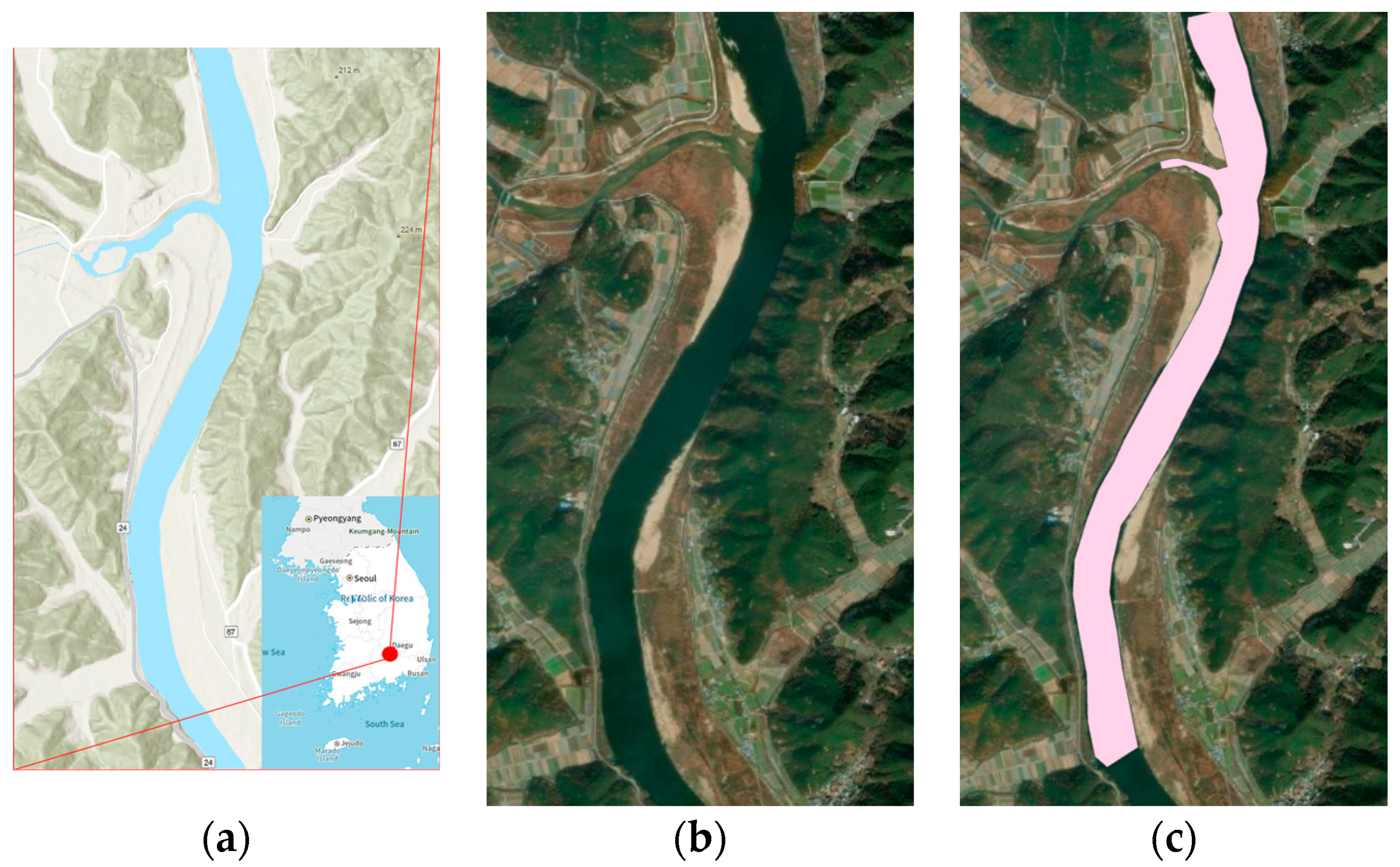
As the target research area, we selected the section from a point 200 m downstream of Hapcheon Changnyeongbo, located in Jangcheon-ri, Ibang-myeon, Changnyeong-gun, South Korea, to another point approximately 300 m upstream of Jeokpo Bridge, passing through the confluence of the Hwang River with the first tributary of the Nakdong River. The target area, where the Hwang River joins the tributary, has complex topographical characteristics, causing the riverbed in this section to fluctuate severely (Figure 1). The main geographical features of the Hwang River confluence are as follows: the Hapcheon Dam is located upstream of the Hwang River, and, hence, the instream flow is determined by the dam’s discharge; furthermore, Hapcheon Changnyeongbo is located upstream of the confluence. The Hwang River watershed mostly consists of agricultural complexes, leading to a high stocking density. The hydrological features are as follows: a riverbed maintenance structure is installed on Cheongdeok Bridge, approximately 1.5 km upstream, to stabilize the flow and riverbeds of the Nakdong River mainstream and Hwang River tributaries; it is a sand-bed river.
The river comprises several tributaries. The mixing pattern at the confluence, where the mainstream and tributaries converge, influences the long-term water quality and mixing characteristics, affecting the water quality characteristics in the downstream section of the confluence. To identify the mixing pattern at the river confluence, it is necessary to perform high-resolution measurements of the confluence section and certain sections of the different water bodies.
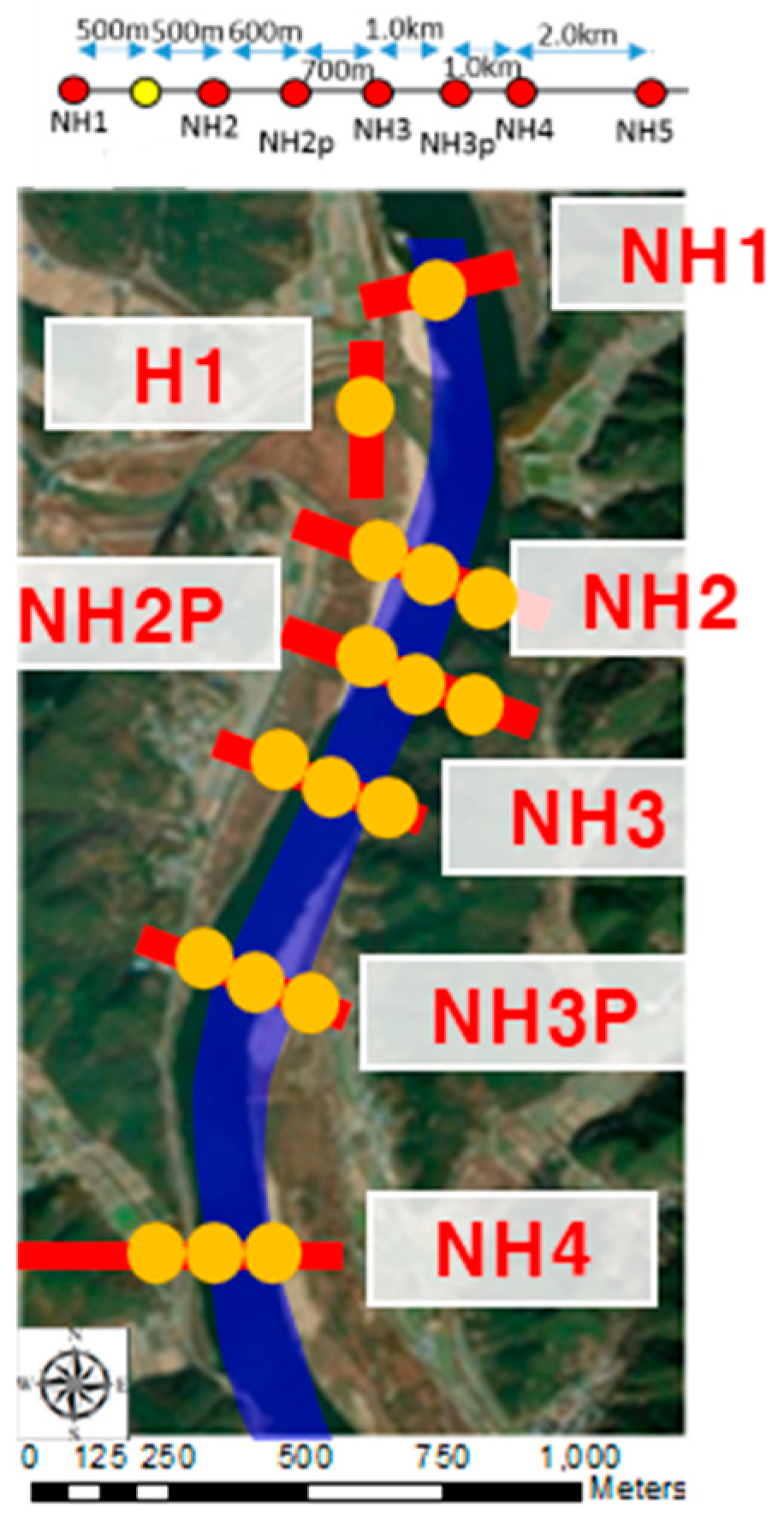
3.2. Measurement Data Acquisition Method and Measurement Routes
Hydrological and water quality data were acquired for the target area using an ADCP and YSI-6600 sensor (Figure 2). The water quality survey of the target section was conducted as follows. Using the YSI-6600 water quality measurement sensor, the survey lines were selected without installing any additional equipment, after which a boat was used to move in the direction perpendicular to the flow while measuring the concentration in real-time. After recording the locations along the selected survey lines via GPS, the hydrologic data and concentration at each survey line were collected, and the vertical distribution of the water quality was measured at the designated points in the river width direction for each cross-section. The ADCP (M9 from SonTek) was installed on the side of the boat on a loading platform, and the hydrologic data were measured under a low-speed operation. The hydrologic data were collected from moving and fixed measurements. In this study, the ADCP was used for the moving measurement method. The hydrologic data were acquired from the upstream and downstream sections of the Nakdong River, Hwang River, and Geumho River, and the confluence of the Nakdong River, Geumho River, and Hwang River. In addition, changes in the flow characteristics of the Nakdong River due to the confluence of the Geumho River and Hwang River were analyzed.
Additionally, the boat was stopped during the cross-sectional movement, and the fixed method employing the YSI-6600 sensor was used to measure the 3D data in the vertical direction of the river. Thus, we used high-resolution 2D surface data and low-resolution vertical data and obtained comprehensive river data via complex monitoring. However, acquiring high-resolution data is tedious, and the measurement time and area are limited; however, if the resolution is reduced, an appropriate interpolation method must be selected to acquire a wide range of data.
Accordingly, an interpolation method was configured to perform a spatial interpolation of the measurement data in the target area. Several interpolation techniques are available, such as the polygon method and IDW [11]. In these deterministic methods, distance is simply used as a factor, and it is not easy to reflect topographical statistical characteristics. In contrast, Kriging is a statistical spatial interpolation technique that quantifies weights based on variograms and considers the spatial autocorrelation between direction, distance, and mathematical functions [12]. It offers the advantages of improved similarity and reliability of spatial interpolation. Moreover, the predictions for each position in the region can be made with greater precision by using the spatial arrangement and variograms, resulting in a more detailed output than those of other interpolation techniques in terms of the visualization data.
In this study, spatial interpolation was performed using each interpolation technique and the same measurements. Based on the 2D spatial interpolation results, it examined the applicability of spatial interpolation to the water quality and surface data at the target area, i.e., the Hwang River confluence.
Kriging was applied using Esri’s ArcGIS Pro software. First, the conditions were configured before generating each layer. The cell sizes of the output data were all set at 3; for extraction, the cell size and projection method were set at the maximum input value and the unit conversion, respectively, and the mask was output and extracted according to the previously set target range. For the natural neighbor technique, because it is impossible to apply the configured conditions and perform the extraction directly in the set range, extraction was performed in the set range by using the “Extract by Mask” technique. Interpolation was performed using Empirical Bayesian Kriging analysis using “Geostatistical Wizard”, a model for the measurement results was selected, and spatial interpolation was performed through numerical optimization of the variogram models described previously.
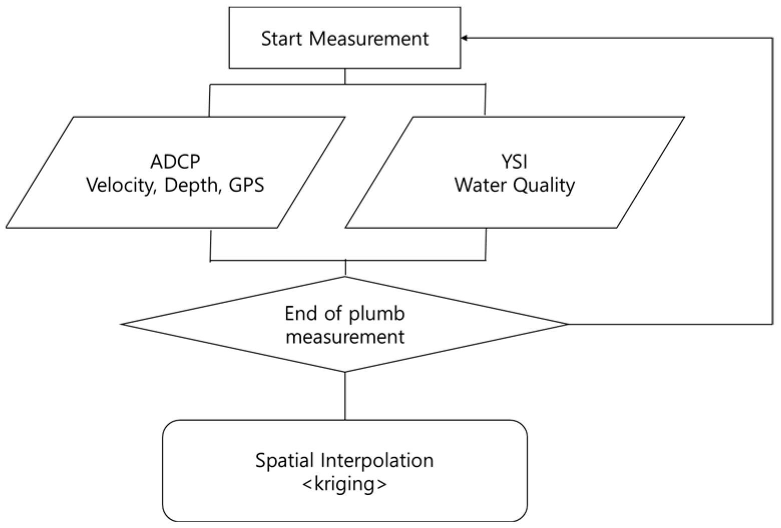
To summarize, it can be organized through a flowchart, as shown in Figure 3. Hydraulic-water quality information is obtained through vertical measurement. Afterwards, interpolation proceeds through the result value obtained through measurement at the next point. During interpolation, interpolation is performed using the Kriging technique mentioned above.
4. Experimental Results
4.1. Three-Dimensional Interpolation through the Selection of the Kriging Technique According to Quantitative Evaluation
In this study, the resolution results of the 3D interpolation of the 2D measurement values were compared. However, because Kriging yielded excellent results for the river confluence for two dimensions, it was not necessary to compare other interpolation techniques to quantify the 3D interpolation. Although the measurement data can be collected at a low resolution, we investigated whether the same interpolation results were obtained for the 3D quantitative evaluation, even if the existing measurement section was deleted. We reduced the existing 3D measurement data and compared how the 2D surface data differed from the 3D cross-sectional z-axis data. The reliability of the Kriging technique was verified via theoretical, visual, and quantitative evaluations of the interpolation using the 2D surface data. We then attempted the 3D evaluation, for which we built the 3D data by interpolating in the z-axis direction from the 2D data.
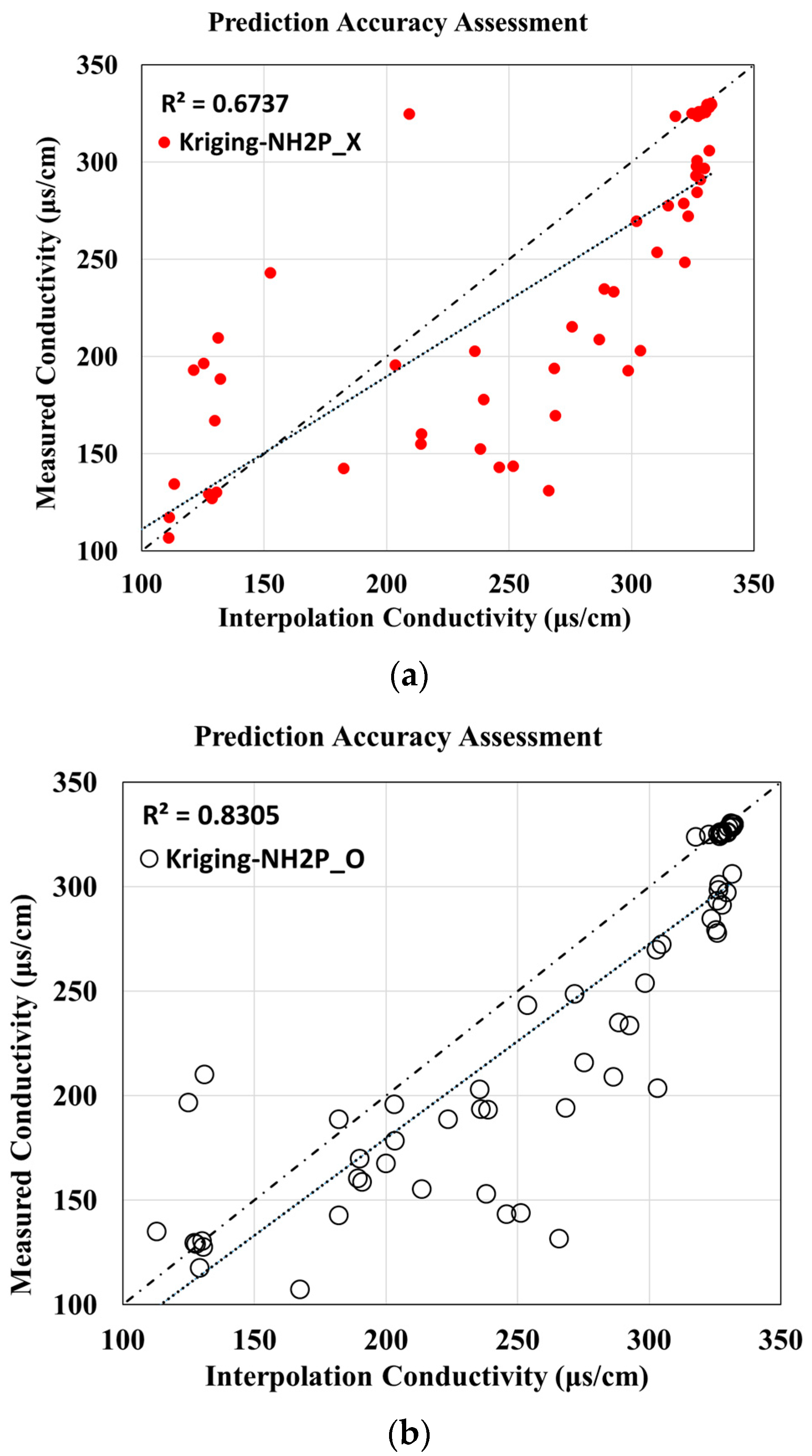
Based on Figure 4, when a comparative analysis was performed as shown in Figure 5, the results are shown in Table 1. Accordingly, the examination was necessary to determine whether the cross-sectional data (i.e., data in the z-axis direction) also have high similarity and correlation. The examination of the results for the high-resolution measurement data reveals an value of 0.8305; although this does not exceed the value for the surface data, it indicates excellent reliability. However, as described in Section 2, the difference in reliability from the surface data is unavoidable, owing to the clear difference in resolution between the hydrological and water quality data. Only 802 vertical data points were used for 8027 surface measurement points, causing the resolution differences. Nevertheless, high reliability and similarity were considered to be achieved based on the and RMSE for the above difference, as shown in Table 1.
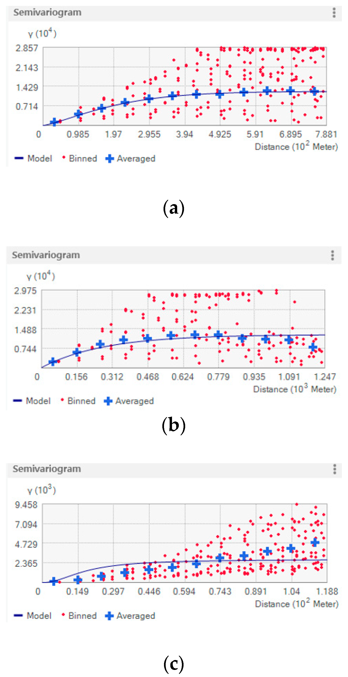
For the data analysis, we first configured the theoretical models using variograms to attempt a numerical optimization of the Kriging technique. Each model was compared and configured to improve the numerical optimization, correlation, and reliability. The “linear model” yielded the most suitable similarity and averages, confirming an even distribution.
Figure 6 shows which model can interpolate with the highest reliability before mapping the entire river. At this time, the variogram was verified by configuring a linear model in which the RMS nearly converges to unity, and the experimentally measured variograms and theoretical modeling results were compared; the condition that “similarity and correlation have high weights in each measurement value” was quantified. This implies that “the predictions of the visualized data are highly reliable”.
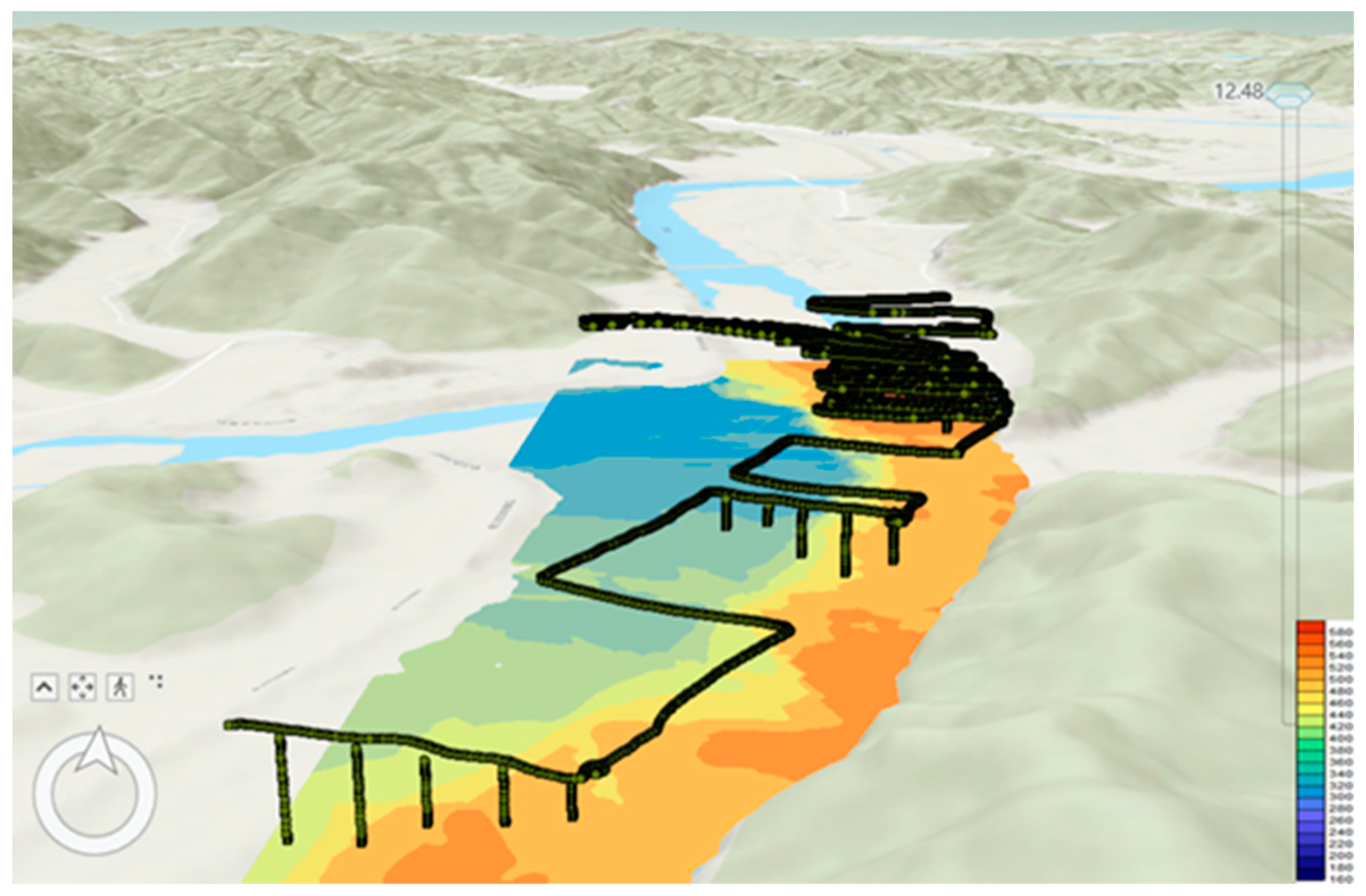
Next, the vertical data and surface data of the measurement points were acquired, as shown in Figure 7. A method that uses an absolute coordinate system and layer-by-layer interpolation may be applied for the 3D interpolation. We compared the methods to determine the one that could most accurately analyze the river confluence section.
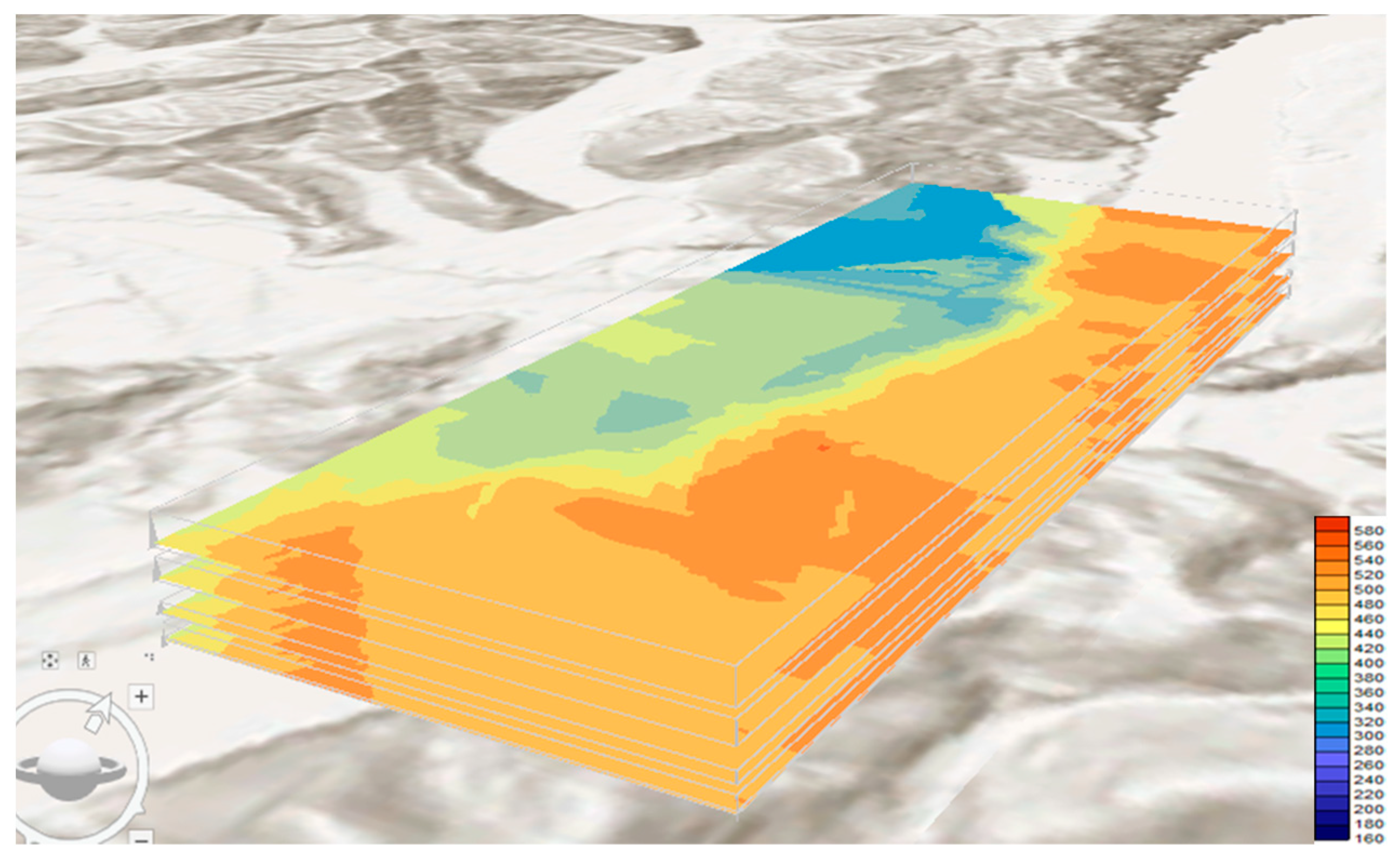
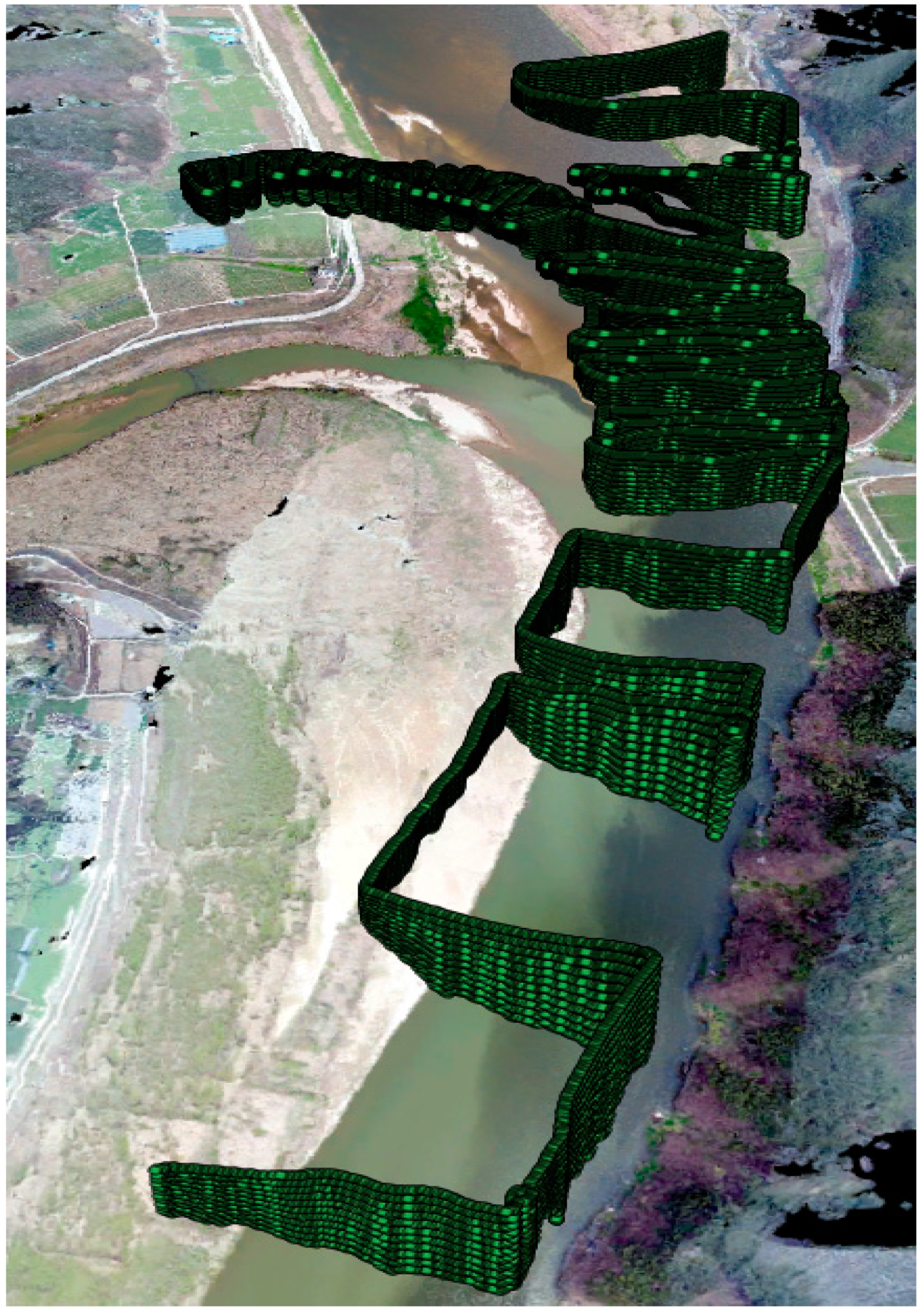
First, a layer for each depth was created, i.e., the layer that interpolates the river data using the absolute coordinates. When creating the layers, the coordinates for the 1 m point on the map were set, and interpolation was performed in the z-axis direction. Figure 8 shows the resulting generated layers. The layers were created at 0.5 m intervals from the surface point. According to the ADCP measurement, the depth of the bottom layer was 4.3 m, which was generated by interpolating 10 layers, including the surface data.
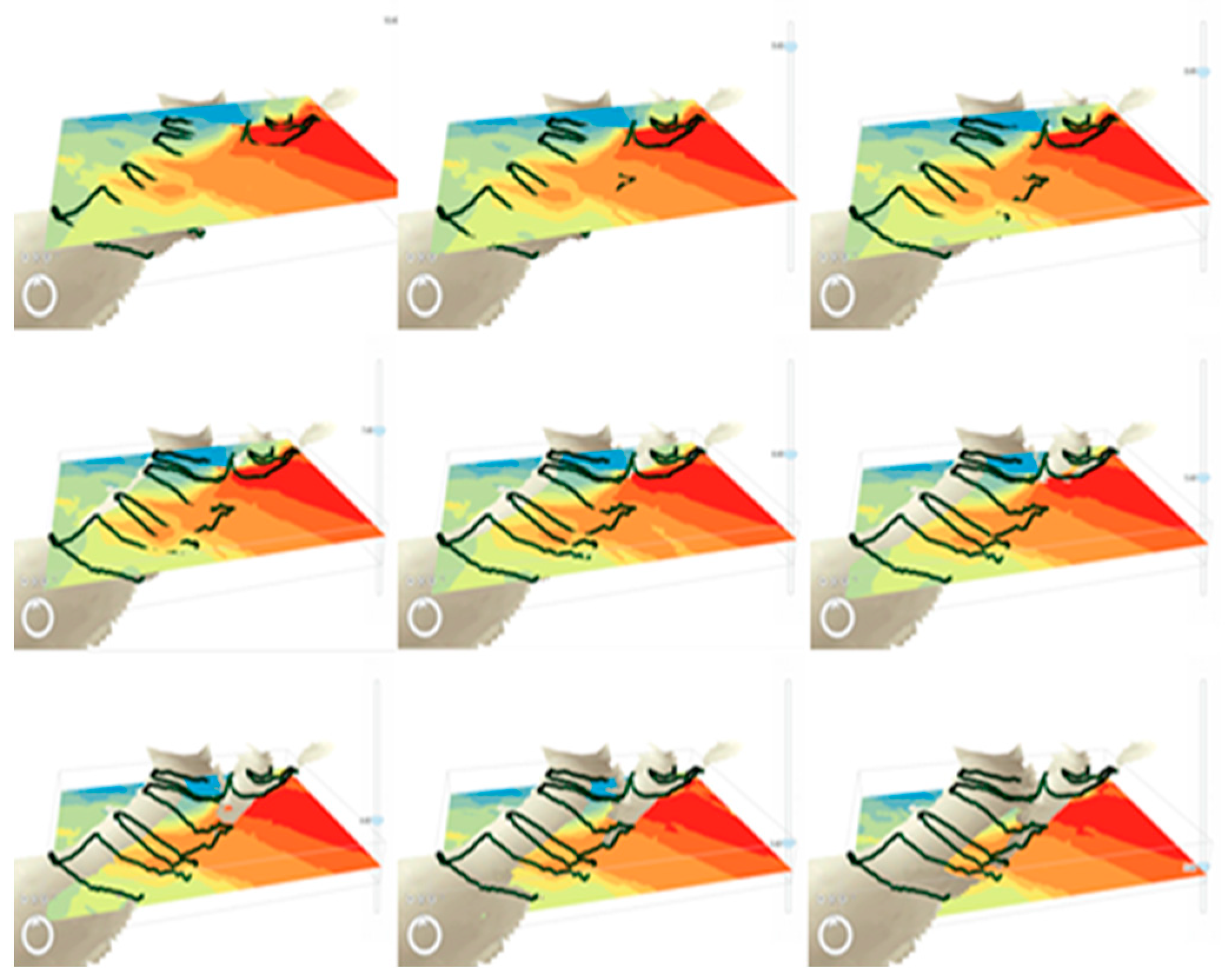
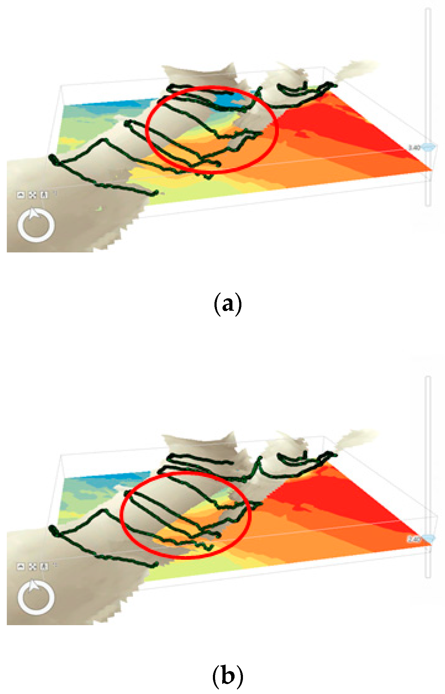
Confirmation was obtained that when the layers were generated for each depth, although continuous interpolations of the layers near the surface and upper water layers were achieved, the interpolation near the riverbed was discontinuous. The depth varies according to the river, and, owing to the characteristics of the confluence, the riverbed structure forms a “ㄱ” shape. However, the layers interpolated for each depth using the absolute coordinates were cut off near the riverbed, as shown in Figure 9 and Figure 10. However, this does not imply that the layers at each depth were interpolated incorrectly. During a study of two water bodies with different river depths by performing interpolation, the limitations of layer generation by depth resulted in discontinuous interpolation while acquiring measurements from the bottom layer of the riverbed, indicating that the layer interpolation direction should be configured differently. The water body depths differ because of the characteristics of the confluence where the tributaries converge with the river. Accordingly, each layer was analyzed separately, as shown in Figure 11.
Owing to the limitations of layer interpolation by depth, layer-by-layer interpolation was performed. Layers were generated for each water layer from the 0.1 m depth point to the 0.9 m depth point, including the surface data. Figure 12 shows the generated data.
After performing the Kriging interpolation from the generated point data, a data insertion procedure was used to insert three categories of water quality (pH, water temperature, and dissolved oxygen (DO)) for the corresponding coordinate points.
Using the created point data, a layer for each water layer was generated to examine the spatial distribution characteristics of the layers from the 0.1 m depth point to the 0.9 m depth point. The generated results were as follows.
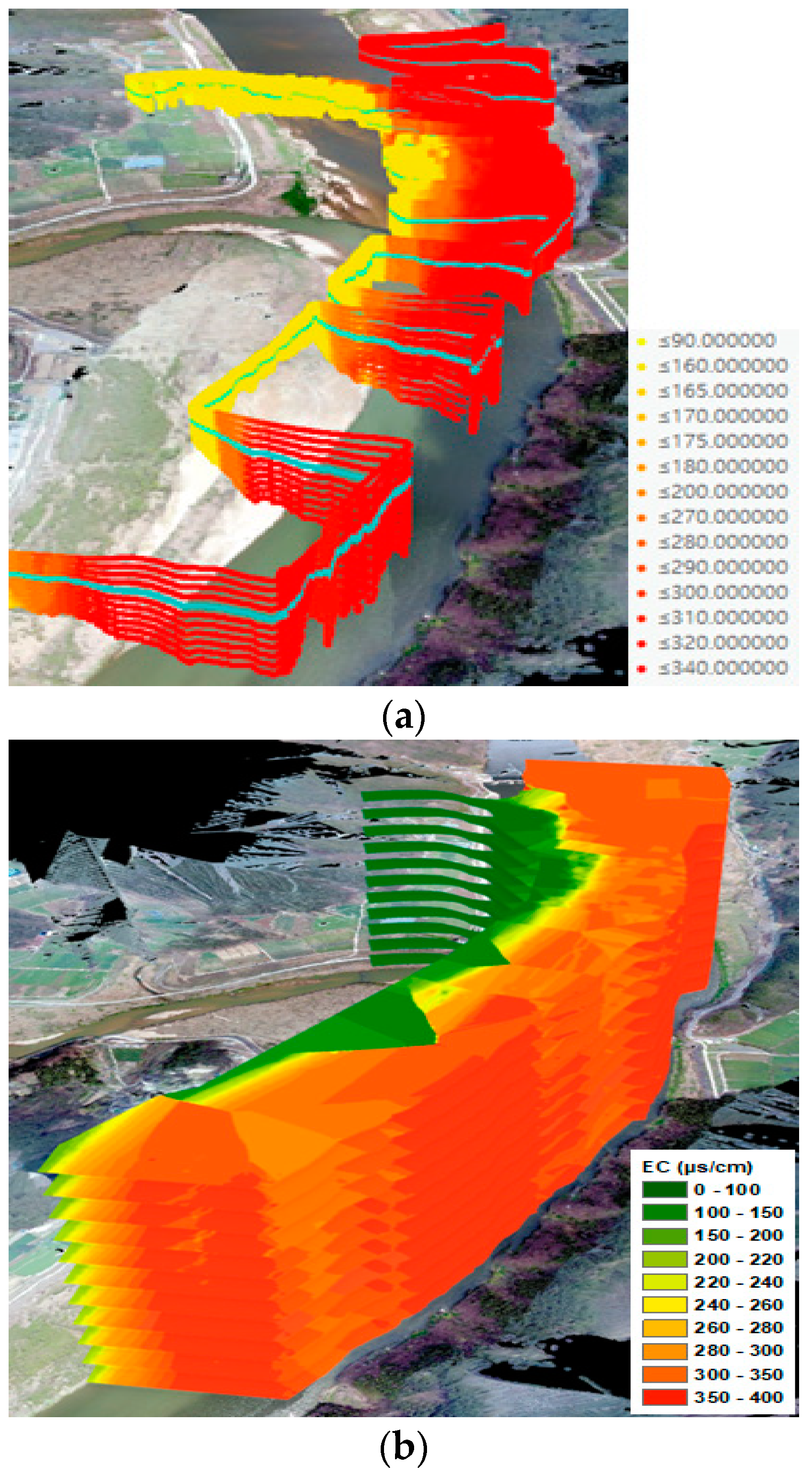
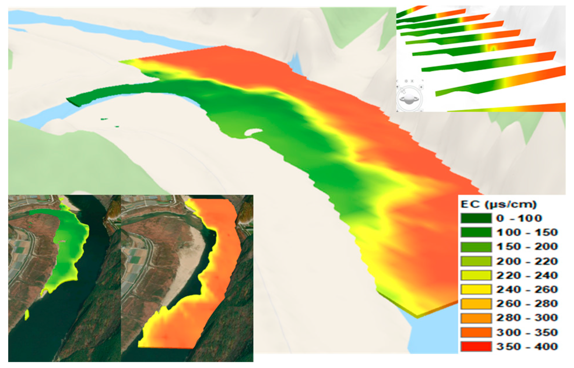
As shown in Figure 12, although point data were created to form the curves, the actual layer interpolation appeared as a flat plane. Because the curved surfaces were generated to appear flat, the discontinuous interpolation resulting from the absolute coordinate depth layers was not included. This indicates that in a section showing the confluence characteristics of different water bodies, it is more advantageous to create a layer for each water layer to efficiently examine the intermixing of the water bodies, which can also improve the reliability of the interpolation. The generated 3D data are shown in Figure 13.
4.2. Comparison of 3D Spatial Interpolation Cross-Sectional Data for Hydrology and Water Quality
In this study, the 3D mixing patterns at the river confluence were analyzed using the previously generated 3D spatial interpolation data.
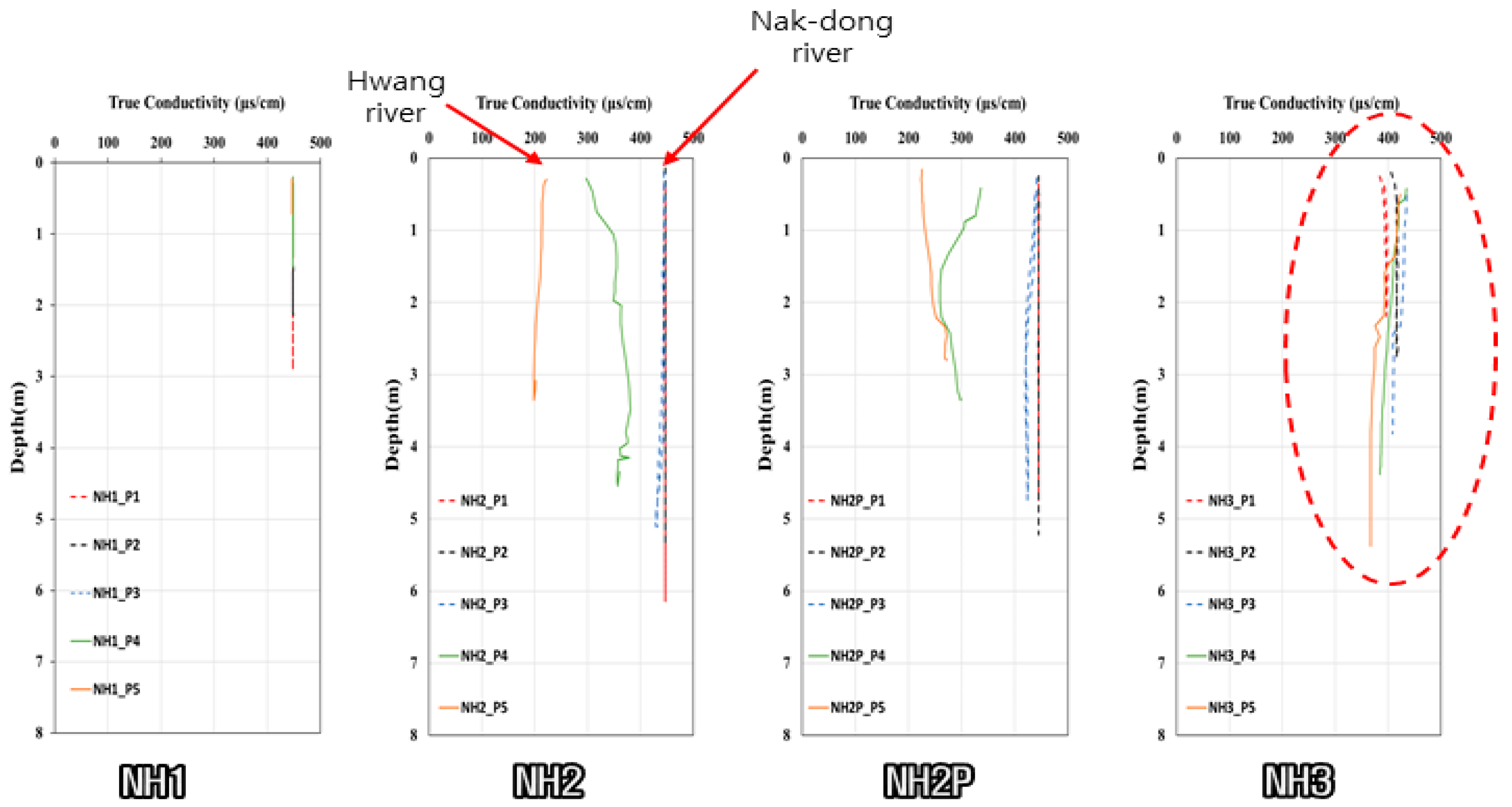
A river confluence is a region where two rivers meet. It is essential to understand the mixing mechanism of the six important sections of a confluence. It is also crucial to analyze the spatial changes that occur when a water body mixes with the main stream according to the various inflow conditions of the tributary. Most prior studies on 3D mixing sections, in which two water bodies mix at a confluence, conducted planar analyses and did not obtain the spatial distributions of the actual 3D mixing sections. Consequently, the data measured in the vertical direction were often analyzed in two dimensions. This 2D analysis resulted in a completely mixed pattern at point NH3 in Figure 14 at the measurement time. Therefore, we compared to determine whether mixing occurred at NH3 in the 3D interpolated data and attempted a 3D mixing analysis.
According to the analysis, the Hwang River converges at NH2. Mixing progresses up to NH2P, and complete mixing of the surface and vertical direction is observed at NH3. Accordingly, we extracted the cross-sectional data using the 3D interpolated data and analyzed whether a pattern similar to the 2D analysis results appeared, as shown in Figure 13.
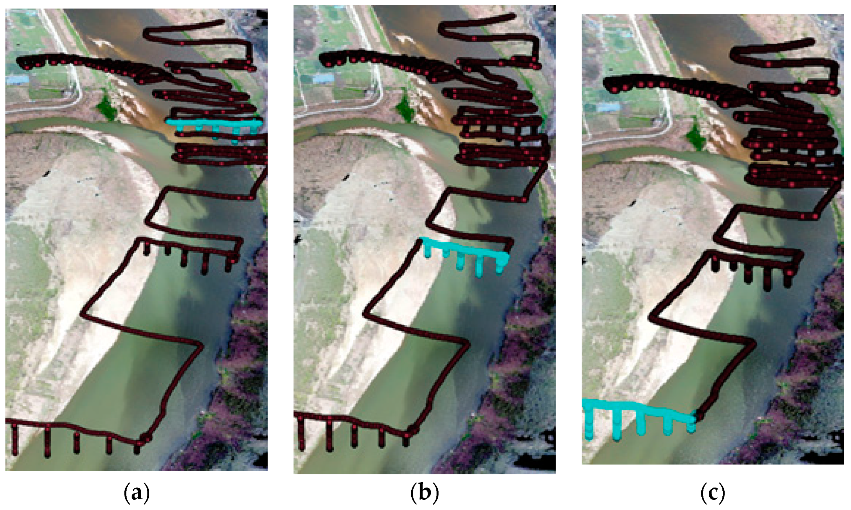
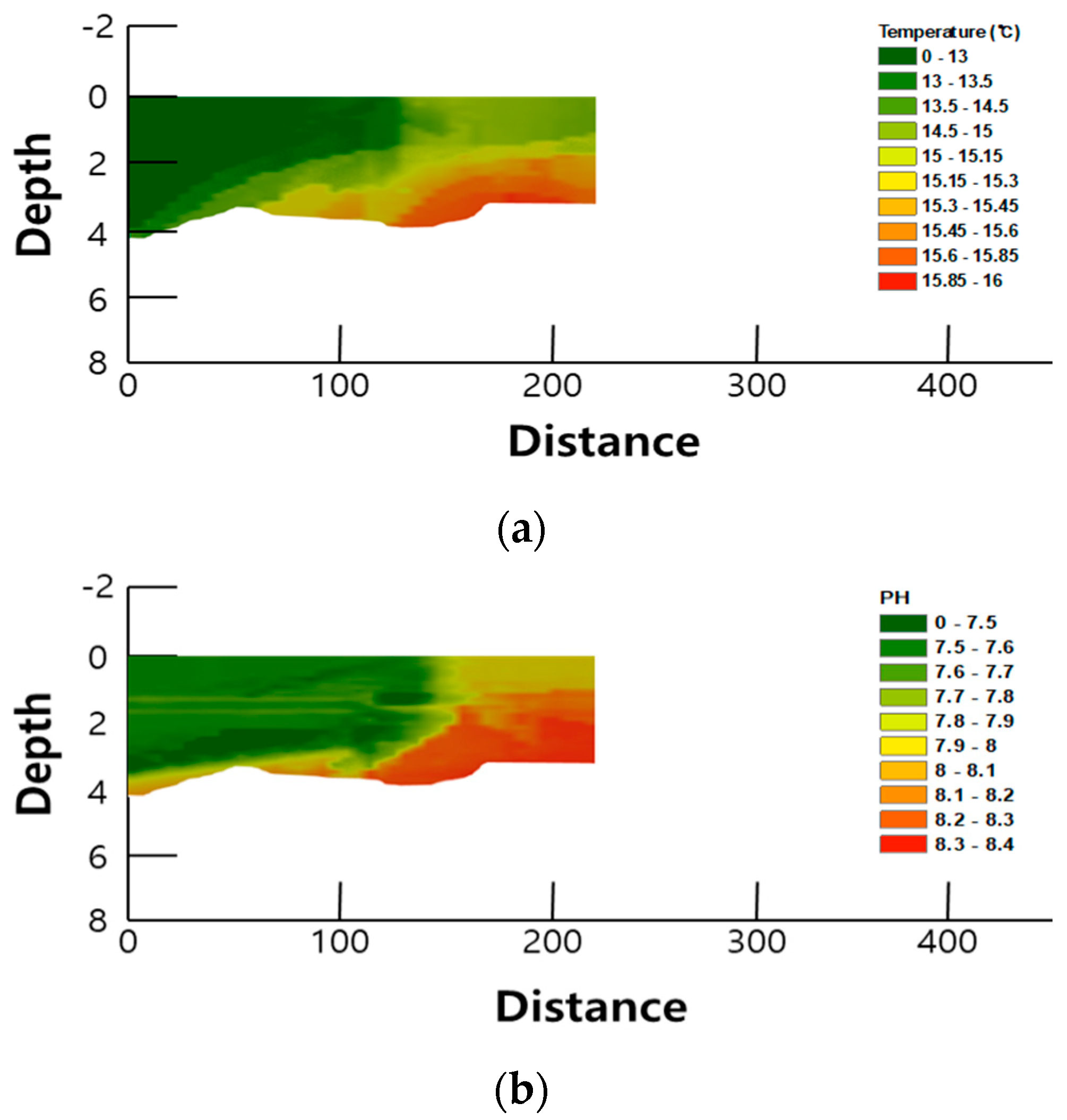
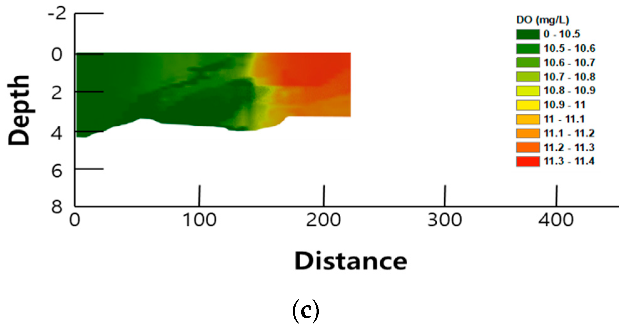
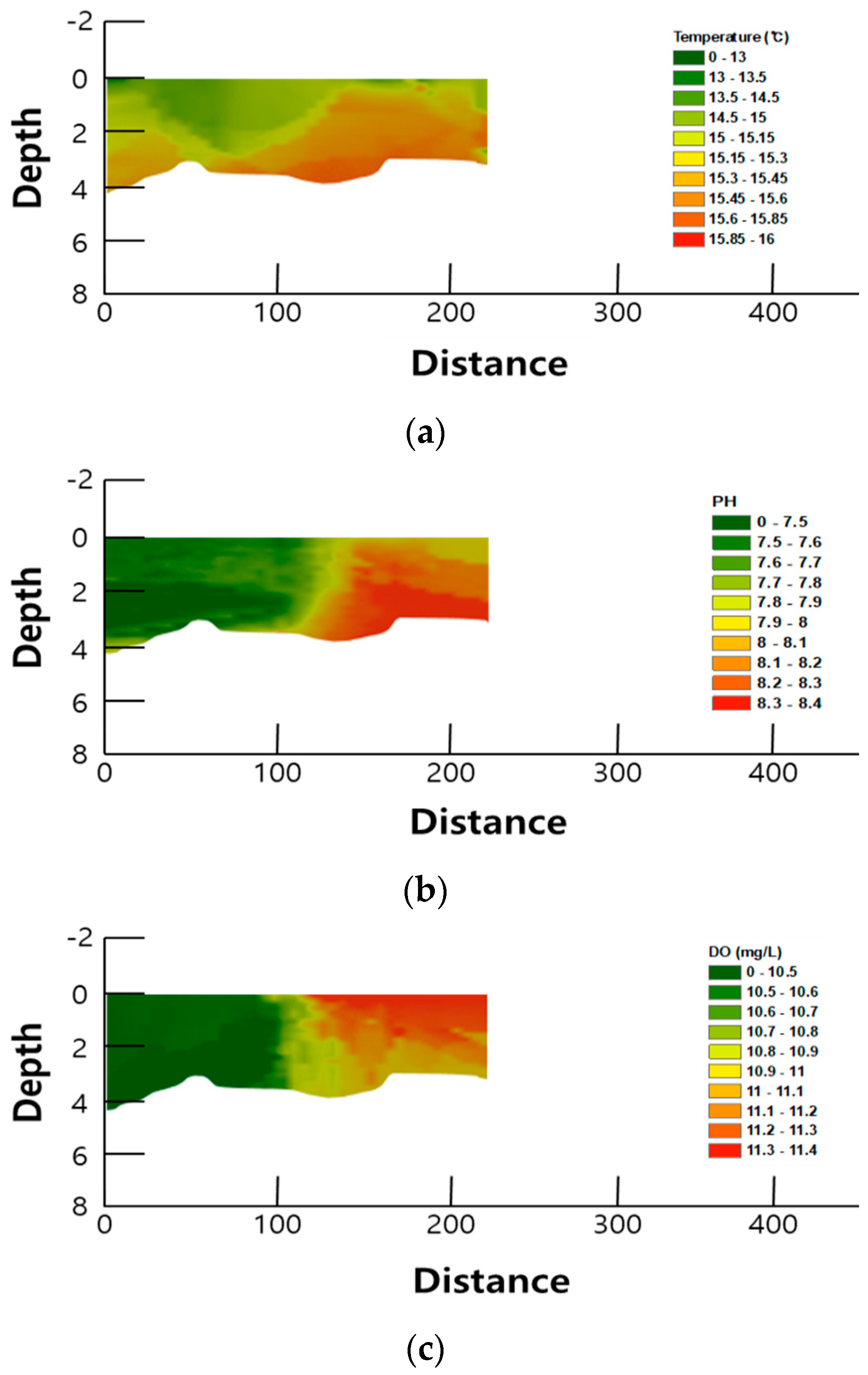
The cross-sectional data were extracted using the interpolated data to observe the hydrological and water quality mixing characteristics in various cross-sections. We randomly selected three survey lines and acquired the cross-sectional data based on the vertical data. The data in the vertical direction were identified to divide the points, and vertical points were set from upstream, as shown in Figure 15. These were acquired using the 3D data interpolated based on the measured data. The water temperature, pH, and DO (mg/L) data were used for the interpolated data analysis. First, the cross-sectional data were partially selected from the combined surface and vertical data. Figure 16, Figure 17 and Figure 18 show the selected vertical interpolation cross-sections at vertical points 1–3, respectively.
When examining the cross-sectional data for each category of water quality in survey line 1, we attempted to identify the mixing pattern using the cross-sectional data for the river width, length, and depth. Regarding water temperature, the influence of the Hwang River extended to approximately 150 m from the left bank to the right bank. It can be visually confirmed that the average water temperature of the Hwang River is approximately 13.5 °C. A water temperature of approximately 15.5 °C; was confirmed for the main stream of the Nakdong River. The pH and DO could also be visually confirmed. Thus, we could visually confirm the water body mixing patterns of the Nakdong River and Hwang River through interpolations of the cross-section of each category of water quality. The results for survey lines 1–3 are summarized in Table 2, Table 3 and Table 4, respectively. The data corresponding to survey lines 2 and 3 were further compared and analyzed.
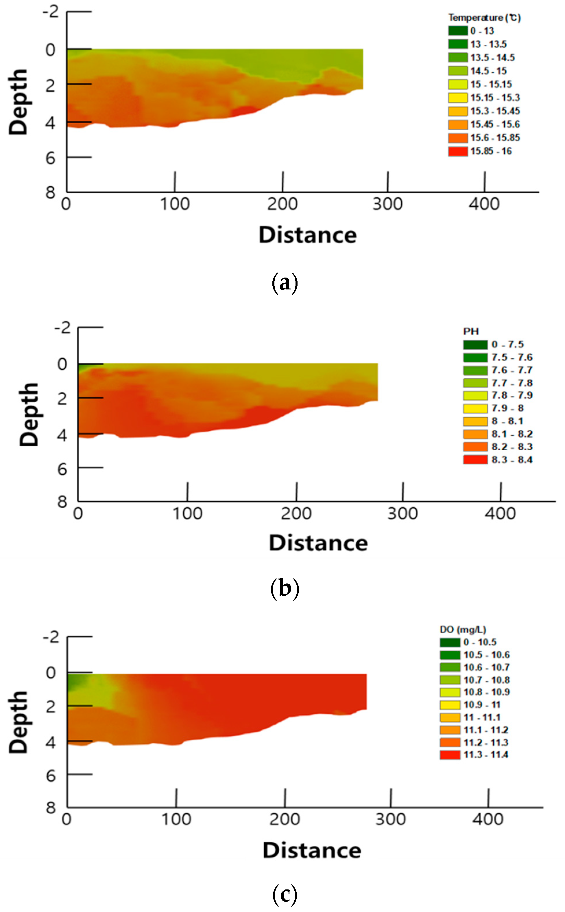
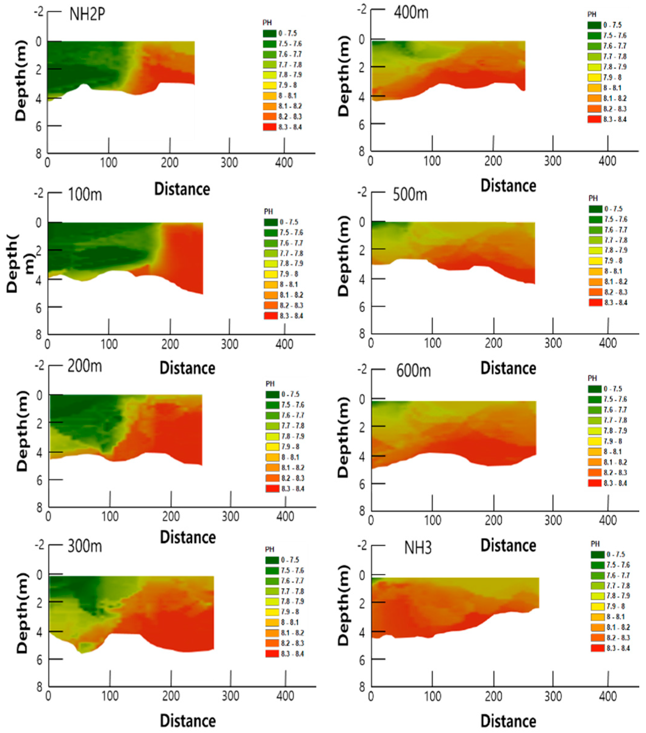
The analysis method applied for survey line 1 was used. We then attempted to extract the data at the cross-sections at 100 m intervals (points NH2P and NH3) if the mixing pattern was not observed before point 3. Approximately 300 m ahead of NH3, the water body gradually displayed a mixing pattern over the entire body, excluding the surface; however, mixing was observed throughout all water layers 100 m before reaching NH3.
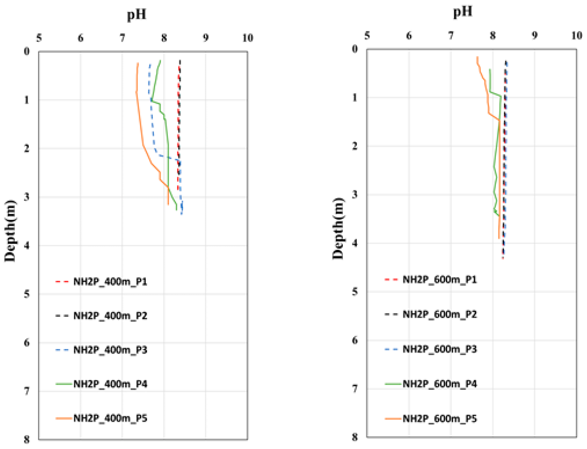
From the interpolated cross-sectional data, the interpolated data for locations corresponding to the vertical measurement points were extracted, and a 2D analysis was performed. As shown in Figure 19, the results were similar to those for the 3D cross-sections. This indicates that mixing water bodies with different properties began at 300 m in front of point NH3; subsequently, mixing occurred 100 m ahead of point NH3 in all vertical layers, excluding the surface.
When the 2D analysis was performed by extracting interpolation data about the measurement point in the vertical direction from the cross-sectional interpolation data, results similar to the 3D cross-section could be confirmed, as shown in Figure 20. At this time, it can also be confirmed that in front of the point about 300 m away from the NH3 point, the mixing of water bodies with different properties is observed and that mixing in the vertical direction occurs in all parts, except for the water surface, 100 m away from the NH3 point. If 3D interpolation data using 2D measurement data can be utilized and cross-sectional information about sidelines can be obtained by acquiring 2D planar data, a more intermediate interpretation may be carried out when understanding the mixing.
Thus, the 3D interpolation data based on 2D measurements enables a more detailed analysis when identifying mixing patterns, whereas only cross-sectional information about the survey line can be obtained using 2D planar data.
5. Conclusions
In this study, water quality measurements at the confluence of the Nakdong River and Hwang River were used to visualize the data based on a comparison of different interpolation techniques, and the corresponding theory and mapping results were obtained. The measurement results were acquired using ADCP and YSI-EXO data. When conducting spatial interpolation according to the flow characteristics of the rivers, the Kriging technique yielded the best performance for the river surface based on a comparison with other techniques. Moreover, applying the Kriging technique and visualizing the data through optimization of the theoretical variogram yielded the result with the “highest similarity” to the predicted value.
Based on the Hwang River measurements described previously, Kriging was used to perform spatial interpolation for the items measured through direct observation. By visualizing each directly observed parameter with Kriging interpolation, it was possible to confirm the formation of the flow of the Hwang River based on the water quality information.
Sensor-based measurements were obtained at the confluence through an integrated and complex monitoring technique. We then compared each interpolation method and conducted visualizations and a pattern analysis using the 3D interpolated data. According to the analytical results, the reliability of the interpolation technique was improved through correlation and similarity evaluation. Finally, we attempted to construct the 3D data through the optimal interpolation technique and illustrated the river mixing patterns.
First, various interpolation techniques were compared herein to determine the most appropriate technique for a section where the rivers converge, which is characterized by complex hydrological characteristics. The Kriging technique yielded excellent visual and quantitative results; hence, it was used to perform the 3D spatial interpolation. Comparing the layer interpolation by depth and layer interpolation by water layer revealed that the layers generated by the water layer in the confluence section were more suitable. Based on these results, voxel layers were created, and based on the cross-sectional 3D data, the river mixing patterns and cross-sectional data relating to hydrology and water quality were compared and analyzed.
Thus, we determined that it is possible to identify the river characteristics by visually confirming the mixing patterns of water bodies with different properties and utilizing the corresponding surface and cross-sectional data.
By mapping the overall hydrological and water quality characteristics of a river through spatial interpolation with consideration of the river flow characteristics, it is possible to examine the factors affecting the water quality, which can be directly observed from the monitoring data. This information contributes to the river design and basic data related to the overall flow of the river.
If it is assumed that the river is steady considering the flow characteristics of the river, the concentration of the confluent river will be constant, and accordingly, when you want to know the starting point at which the river is mixed, you can interpolate into a 3D rather than a 2D measurement result. Based on the results, you can more easily identify the target location. In particular, it is possible to calculate the mixing distance of a river or analyze the mixing behavior through 3D interpolation.
Finally, although 2D data can be interpreted by analyzing only the cross-sectional measurement data, the mixing behavior can be analyzed in greater detail using 3D interpolation data. The 3D interpolation data can be used in various studies by employing various spatial interpolation analysis methods and hydro-engineering, such as identifying aquatic ecological health and mixing patterns. In addition, we suggest river route setting as a research topic for future studies.
Author Contributions
Conceptualization, C.H.L., Y.D.K. and D.S.K.; methodology, S.L. and Y.D.K.; software, C.H.L. and K.D.K.; validation, C.H.L. and K.D.K.; formal analysis, C.H.L. and K.D.K.; investigation, C.H.L. and K.D.K.; resources, C.H.L. and K.D.K.; data curation, S.L., D.S.K. and Y.D.K.; writing—original draft preparation, C.H.L. and Y.D.K.; writing—review and editing, C.H.L. and Y.D.K.; visualization, C.H.L. and K.D.K. All authors have read and agreed to the published version of the manuscript.
Funding
This research was funded by the research fund of the aquatic ecological health technology development project of the Ministry of Environment, grant number 2021003030005.
Data Availability Statement
Software name: ArcGIs Pro 3.0. Developer: ESRI. First-year available: 2022. Hardware requirements: PC. Software requirements: Window. Program language: Python. Program Size: 32 GB. Availability: https://www.esri.com/. License: ArcGIS Pro Educational Academic Departmental Medium Single Use Annual Subscription. Archive with data from benchmarking: None. Size of archive: None.
Conflicts of Interest
The authors declare no conflict of interest.
References
- Park, Y.; Cho, K.; Cho, C. Seasonal variation of water temperature and dissolved oxygen in the Youngsan Reservoir. J. Korean Soc. Water Environ. 2008, 24, 44–53. [Google Scholar]
- Song, E.S.; Cho, K.A.; Shin, Y.S. Exploring the dynamics of dissolved oxygen and vertical density structure of water column in the Youngsan Lake. J. Environ. Sci. Int. 2015, 24, 163–174. [Google Scholar] [CrossRef] [Green Version]
- Baek, S.; Seong, C.; Choe, S.; Park, Y.; Kim, M. Mobile water quality monitoring system using ion-selective-electrodes. J. Inst. Electron. Inf. Eng. 2018, 55, 29–38. [Google Scholar]
- Lee, J.; Kim, Y. Location suitability assessment on marine afforestation using habitat evaluation procedure (HEP) and 3D kriging: A Case Study on Jeju, Korea. J. Econ. Geog. Soc. Korea 2014, 17, 771–785. [Google Scholar]
- Koo, H.D.; Chung, D.K.; Yoo, H.H. Analysis of 3D data structuring and processing techniques for 3D GIS, Korean Society of Surveying. Geod. Photogramm. Cartogr. 2004, 39, 375–382. [Google Scholar]
- Lee, J.O.; Park, U.Y.; Yang, Y.B.; Kim, Y.S. 3D modelling shape embodiment and efficiency analysis of reservoir that using RTK-GPS and E/S. J. Korean Soc. Geospat. Inf. Sci. 2005, 13, 11–17. [Google Scholar]
- Parsons, D.R.; Best, J.L.; Lane, S.N.; Orfeo, O.; Hardy, R.J.; Kostaschuk, R. Form roughness and the absence of secondary flow in a large confluence-diffluence, Rio Paraná, Argentina. Earth Surf. Process. Landf. 2007, 32, 155–162. [Google Scholar] [CrossRef]
- Lee, H.E.; Lee, C.J.; Kim, Y.J.; Kim, W. Analysis of vertical velocity distribution in natural rivers with ADCPs. Proc. Korea Water Resour. Assoc. Conf. 2009, 5, 1865–1869. [Google Scholar]
- Hwang, K.S.; Park, D.S.; Jung, W.S. Spatial Reservoir Temperature monitoring using thermal line sensor. Proc. Korea Water Resour. Assoc. Conf. 2006, 13, 1002–1006. [Google Scholar]
- Lee, C.H.; Park, J.G.; Kim, K.D.; Lyu, S.W.; Kim, D.S.; Kim, Y.D. Two-dimensional spatial distribution analysis using water quality measurement results at river junctions. J. Korean Soc. Civ. Eng. 2022, 13, 11–179. [Google Scholar]
- Kim, D.H.; Lyu, D.W.; Choi, Y.M.; Lee, W.J. Application of Kriging and inverse distance weighting method for the estimation of geo-layer of Songdo Area in Incheon. J. Korean Geotechn. Soc. 2010, 26, 5–19. [Google Scholar]
- Cho, H.L.; Jeoung, J.C. A Study on spatial and temporal distribution characteristics of coastal water quality using GIS. Spatial Inf. Res. 2006, 14, 223–234. [Google Scholar]
Figure 1.
Target research area. (a) Description for the first panel. (b) Description for the middle panel. (c) Description for the last panel.
Figure 1.
Target research area. (a) Description for the first panel. (b) Description for the middle panel. (c) Description for the last panel.

Figure 2.
Measurement route and survey line selection configuration.

Figure 3.
Research method flow chart.

Figure 4.
Quantitative evaluation of the interpolation according to resolution differences (a) with and (b) without the measurement results.
Figure 4.
Quantitative evaluation of the interpolation according to resolution differences (a) with and (b) without the measurement results.

Figure 5.
Interpolation comparison according to resolution differences.

Figure 6.
Comparison of theoretical models using the Kriging technique. (a) Exponential, (b) spherical, and (c) Gaussian models.
Figure 6.
Comparison of theoretical models using the Kriging technique. (a) Exponential, (b) spherical, and (c) Gaussian models.

Figure 7.
Three-dimensional measurement path for the merged Hwang River junction.

Figure 8.
Layer generation by depth using absolute coordinates.

Figure 9.
Layers according to absolute coordinate depth.

Figure 10.
Layer discontinuity at (a) 4 and (b) 4.5 m.

Figure 11.
Three-dimensional point data generation according to grid.

Figure 12.
Layer discontinuity. (a) Three-dimensional point data generation; (b) layers interpolated by a water layer.
Figure 12.
Layer discontinuity. (a) Three-dimensional point data generation; (b) layers interpolated by a water layer.

Figure 13.
Generated 3D spatial data.

Figure 14.
Two-dimensional analysis results in the vertical direction for different measurement points.
Figure 14.
Two-dimensional analysis results in the vertical direction for different measurement points.

Figure 15.
Illustration of selected points along the research target area. (a–c) Vertical points 1–3, respectively.
Figure 15.
Illustration of selected points along the research target area. (a–c) Vertical points 1–3, respectively.

Figure 16.
Cross-sectional data of water quality at vertical point 1. (a) Water temperature (°C), (b) pH, and (c) DO (mg/L).
Figure 16.
Cross-sectional data of water quality at vertical point 1. (a) Water temperature (°C), (b) pH, and (c) DO (mg/L).


Figure 17.
Cross-sectional data of water quality at vertical point 2. (a) Water temperature (°C), (b) pH, and (c) DO (mg/L).
Figure 17.
Cross-sectional data of water quality at vertical point 2. (a) Water temperature (°C), (b) pH, and (c) DO (mg/L).

Figure 18.
Cross-sectional data of water quality at vertical point 3. (a) Water temperature (°C), (b) pH, and (c) DO (mg/L).
Figure 18.
Cross-sectional data of water quality at vertical point 3. (a) Water temperature (°C), (b) pH, and (c) DO (mg/L).

Figure 19.
Generation of 2D analysis data using 3D interpolation data.

Figure 20.
Extracted cross-sectional data at 100 m intervals using 3D interpolation data.


Table 1.
RMSE and R2 for each interpolation method.
| Kriging Method | |||
|---|---|---|---|
| NH2P-O | NH2P-X | ||
| R2 | RMSE | R2 | RMSE |
| 0.8305 | 19.7 | 0.6737 | 44.2 |
Table 2.
Cross-sectional comparison of water quality at survey line 1.
| Survey Line 1 | |||
|---|---|---|---|
| Range of influence of Hwang River | 150 m | 155 m | 153 m |
| Category | Water temperature (°C) | pH | DO (mg/L) |
| Hwang River | 13.5 | 7.6 | 10.55 |
| Nakdong River | 15.5 | 8.3 | 11.25 |
Table 3.
Cross-sectional comparison of water quality at survey line 2.
| Survey Line 2 | |||
|---|---|---|---|
| Range of influence of Hwang River | 130 m | 120 m | 105 m |
| Category | Water temperature (°C) | pH | DO (mg/L) |
| Hwang River | 14.75 | 7.65 | 10.55 |
| Nakdong River | 15.55 | 8.3 | 11.25 |
Table 4.
Cross-sectional comparison of water quality at survey line 3.
| Survey Line 3 | |||
|---|---|---|---|
| Range of influence of Hwang River | 20 m | 25 m | 25 m |
| Category | Water temperature (°C) | pH | DO (mg/L) |
| Hwang River | - | 7.5 | 10.6 |
| Nakdong River | 15.6 | 8.3 | 11.5 |
Disclaimer/Publisher’s Note: The statements, opinions and data contained in all publications are solely those of the individual author(s) and contributor(s) and not of MDPI and/or the editor(s). MDPI and/or the editor(s) disclaim responsibility for any injury to people or property resulting from any ideas, methods, instructions or products referred to in the content. |
© 2023 by the authors. Licensee MDPI, Basel, Switzerland. This article is an open access article distributed under the terms and conditions of the Creative Commons Attribution (CC BY) license (https://creativecommons.org/licenses/by/4.0/).
Share and Cite
MDPI and ACS Style
Lee, C.H.; Kim, K.D.; Lyu, S.; Kim, D.S.; Kim, Y.D. Analysis of Mixing Patterns of River Confluences through 3D Spatial Interpolation of Sensor Measurement Data. Water 2023, 15, 925. https://doi.org/10.3390/w15050925
AMA Style
Lee CH, Kim KD, Lyu S, Kim DS, Kim YD. Analysis of Mixing Patterns of River Confluences through 3D Spatial Interpolation of Sensor Measurement Data. Water. 2023; 15(5):925. https://doi.org/10.3390/w15050925
Chicago/Turabian StyleLee, Chang Hyun, Kyung Dong Kim, Siwan Lyu, Dong Su Kim, and Young Do Kim. 2023. "Analysis of Mixing Patterns of River Confluences through 3D Spatial Interpolation of Sensor Measurement Data" Water 15, no. 5: 925. https://doi.org/10.3390/w15050925
Note that from the first issue of 2016, this journal uses article numbers instead of page numbers. See further details here.