
A New Decision Support Tool for Evaluating the Impact of Stormwater Management Systems on Urban Runoff Pollution

Aquafin NV, Dijkstraat 8, B-2630 Aartselaar, Belgium
*
Author to whom correspondence should be addressed.
Water 2023, 15(5), 931; https://doi.org/10.3390/w15050931
Submission received: 16 January 2023
/
Revised: 10 February 2023
/
Accepted: 23 February 2023
/
Published: 28 February 2023
(This article belongs to the Special Issue Modeling and Simulation of Urban Drainage Systems)
Abstract
:Stormwater runoff is often discharged untreated into receiving waters, a process that is widely recognized as a threat to water quality. To protect water bodies, tools are needed to assess the risk of urban runoff pollution. In this work, a new tool is presented that can be used to model the concentration of the most frequent pollutants in urban runoff, i.e., Zn, Cu, Pb, PAH(1)6, TN, and TP, based not only on the surface type but also on other inputs such as the amount of traffic or the building type. The tool also includes a simple model to evaluate the impact of different SUDS types. The water quality model was evaluated by measurement campaigns in separate sewer systems of a few small catchments in Flanders. The model was able to reproduce the observed time-dependent spread in concentrations in a satisfactory manner. Furthermore, the model also allowed for the attribution of differences in heavy metal concentrations in catchments very similar to the building types. These are clear improvements compared to previous model approaches.
1. Introduction
Stormwater runoff is often discharged untreated into receiving waters, a process that is widely recognized as a threat to their water quality [1,2,3,4]. Urban runoff pollution is expected to worsen with climate change and an increasing population [4,5]. The European Union has already begun to adopt more stringent stormwater quality standards. Sustainable urban drainage systems (SUDS) are emerging as a promising strategy to reduce this pollution and other impacts of climate change, such as flooding and drought. To protect water bodies, tools are needed to assess urban runoff pollution and to evaluate the performance of different treatment strategies such as SUDS.
Urban runoff quality can be assessed by the current catchment modeling tools (e.g., SWMM, ICM, MIKE URBAN), which have also incorporated most types of SUDS as standard modules. Next to the standard software, several other tools have been developed to model urban runoff pollution and SUDS, e.g., MUSIC, P8-UCM, WinSLAMM, and GIFMOD [5,6].
In many tools such as SWMM, MIKE URBAN, or GIFMOD, urban runoff quality can be modeled by a deterministic approach, assuming pollutant build-up during dry weather and pollutant wash-off during storm events for different categories of land use. However, the parameters of the build-up and wash-off curves have to be defined by the user. Many studies have tried to estimate the build-up and wash-off dynamics for different types of surfaces, at both small and larger catchment scales, with varying levels of success [7]. Unfortunately, the ranges of the model parameters are very wide depending on the experimental study [7,8,9,10,11,12,13]. For small-scale studies, the wash-off is well predicted and mainly dependent on the rainfall characteristics. Although build-up is commonly understood to depend on the number of antecedent dry days, many researchers have noticed that the build-up rates and loads are site specific and dependent on factors such as the road surface condition and traffic volume [8,9,11]. Nevertheless, in many studies, the build-up parameters are determined by drainage surface type (e.g., roof, highway, road, residential), without taking into account these other factors. Other sources that have been reported to contribute to the pollution, such as atmospheric deposition or anthropogenic activities (e.g., pets and wildlife, gardening) [4], are ignored in these studies.
Other tools, such as WinSLAMM, P8-UCM, or StormTac [14], circumvent this problem by using a statistical approach to assess urban runoff quality. Here, an average pollutant concentration is assumed for different types of surfaces (roofs, streets) based on a large number of studies. Again, site-specific characteristics such as traffic volume are ignored. Further, these tools fail to predict peak emissions, which is important for assessing ecotoxicity on surface waters.
On the other hand, several tools have been developed to estimate pollutant loads (instead of concentrations) more accurately. The Australian model “Risk Assessment of road stormwater runoff” (RSS) predicts the copper and zinc loads from road runoff and other non-road (urban) sources, based on the annual vehicle kilometers travelled and the road level of service [15]. However, it is specifically designed for zinc and copper pollution on roads and does not include other pollutants or site-specific information from other sources.
Several EU member states have developed more complete webtools to comply with the mandatory inventory of emissions, losses, and discharges of priority hazardous substances at the EU level (Directive 2008/105/EC EQS) [16,17,18,19]. For instance, the Flemish WEISS and German MoRE are tools to assess the pollution load from different sources, such as industry, agriculture, traffic, and domestic sources to waterbodies as accurately as possible. The Flemish WEISS tool contains factors that predict the emissions of the most relevant pollution sources in urban runoff as described in [4], such as atmospheric deposition, traffic, or the corrosion of building materials [17,18,19]. Similar to the RSS model, WEISS calculates the pollution from roads based on the road type and traffic volume. Furthermore, the tool also uses site-specific information for other sources, such as building types, to assess the corrosion of building materials.
These tools predict pollutants loads, which can easily be converted into concentrations using rainfall data. In this way, the rain-dependent time dynamics of concentrations are included, which is a clear advantage compared to the common statistical approach. Furthermore, as no calibration is needed, the tools are easier to use than the build-up/wash-off models. Although the WEISS/MoRE tools are probably not capable of a very accurate prediction of the runoff quality in different storm events, they may be well fit to compare the pollution from different catchments for decision-making purposes. To the best of the authors’ knowledge, the approach has not yet been used or validated for this purpose.
In this contribution, we present an easy-to-use tool, aquaSens, in which the pollutant build-up for small catchments is calculated by the WEISS model, complemented with other publications to cover a wide range of the most common stormwater pollutants. The pollutant load is converted into a concentration using wash-off equations. This stormwater quality model is validated by measurements in four small Flemish catchments.
The aquaSens tool also includes a sedimentation model to evaluate the impact of SUDS. Different SUDS can be selected and modeled in one run, so that their impact (both hydrological and water quality) can easily be compared. Different dimensions or configurations of the SUDS can also be modeled and compared in one run.
The tool can be used by decision makers, for instance, to prioritize the surfaces that need to be treated before discharge to surface waters and to select treatment strategies such as SUDS.
The tool is designed to model small catchments. However, the water quality model is basically a build-up/wash-off model, so it can also be implemented in standard hydrological tools to model larger catchments.
2. Materials and Methods
2.1. Description of the aquaSens Tool
2.1.1. Model Input
The model requires the manual input of the project details, such as the areas of all streets, roofs and other impervious or pervious surfaces, the soil infiltration capacity, and the groundwater level. The tool calculates the runoff from the pervious and impervious areas of the project. Both the amount of runoff (Section 2.1.2) and the quality of the runoff (Section 2.1.3) are calculated.
Furthermore, the tool automatically returns a list of SUDS types that can be applied in the project to reduce the runoff and to improve the runoff quality. The following extended set of treatments is included: green roofs, rainwater harvesting tanks, storage tanks, infiltration wells, infiltration basins, bioswales, infiltration trenches, vertical and horizontal infiltration pipes, soakaway crates, infiltration street gullies, permeable paving, street trees, and a reduction in impervious surfaces.
A set of discrete default values for the dimensions of the SUDS are assumed, based on the inputs (for instance, the available space), local regulations, and standards of manufacturers. These values can also be adjusted by the user.
2.1.2. Runoff Calculation
For design purposes, precipitation (5 min) and evaporation (daily) data are provided by the Belgian Meterological Institute [20]. For validation of the water quality model, rainfall data from rain gauges was used.
The runoff is calculated by taking into account depression storage and a fixed runoff coefficient. The depression storage D of impervious surfaces is calculated from the terrain slope S by the following equation, which is also implemented in Infoworks ICM:
A runoff coefficient of 0.8 was assumed for all impervious surfaces. This value can be adjusted by the user.
No routing of the rainfall over the surface is included, so the tool can only be used for small catchments.
2.1.3. Runoff Quality Calculation
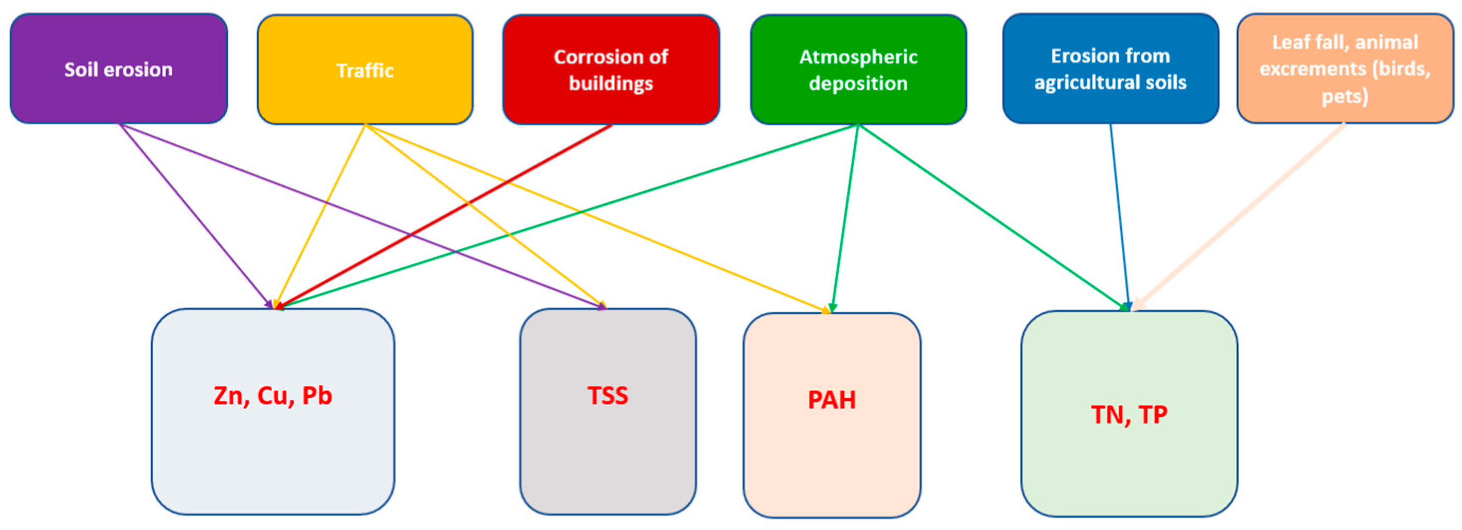
The pollutants and pollutant sources that are included in the aquaSens tool are shown in Figure 1. These cover the most common sources described in literature [4]. The pollution load from these sources is calculated by the Flemish Water Emission Inventory Support System (WEISS) [17,18,19] complemented with other publications, as explained further in this section.
Different sources, including industry, traffic, and agriculture, emit pollutants into the air, which eventually end up in urban runoff by wet and dry deposition. In WEISS, these contributions are all collected under the source “atmospheric deposition”. Details about the computation of this contribution can be found in [17,18,19].
The source “corrosion of building materials” contributes to zinc, copper, and lead pollution in urban runoff. In the WEISS tool, this contribution is calculated by emission factors that reflect the expected emissions for each building type (g/building/year) [21] (Table A2). These numbers are based on a questionnaire among Flemish building companies about the amount of zinc, copper, and lead that is typically used in different types of buildings [21]. The reported emission factors agree well with those reported in other studies [22,23]. TSS concentrations in roof runoff are reported to be very low [24,25] and are ignored in the tool. PAH leaching from roof materials is also ignored. Although PAH leaching from bituminous or EPDM roofing has been reported, street runoff was identified as the most significant contributor of PAHs in urban areas [26,27,28,29,30].
Runoff from roads is polluted with heavy metals and PAHs by road wear, tire wear, and oil leakage. In the WEISS tool, the emission factors for these contributions are defined by vehicle and road type (in g/vehicle km) [17,18,19] (Table A3). The emission of pollutants from traffic into the atmosphere is not included in these emission factors but is taken up in the source atmospheric deposition.
The pollutant TSS is not contained in the WEISS tool. Here, it is assumed that the main TSS pollution in road runoff is caused by tire and road wear, with the emission factors given in reference [31]. These agree well with other studies [32]. For pervious areas, such as agriculture or construction sites, typical TSS emission factors were taken from reference [33].
WEISS only includes the source “agriculture” for the occurrence of TN and TP in urban runoff. However, atmospheric deposition, leaf fall and animal fecal matter are also major contributions. The emission factors of these contributions (in g/ha/year) were taken from reference [34] and are shown in Table A4.
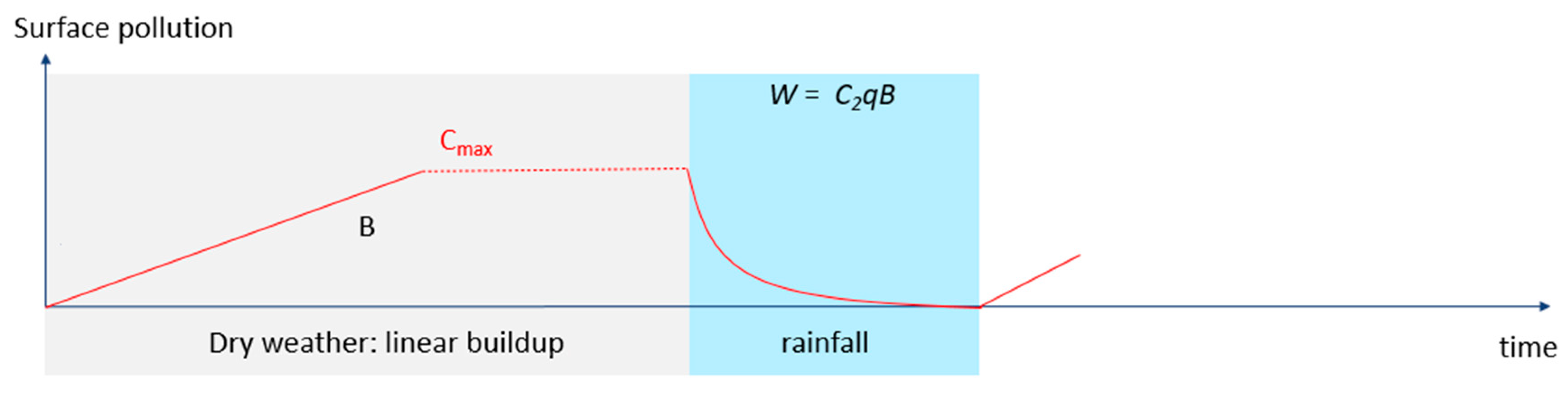
The WEISS method returns a total annual load in g/year. This load should be converted to a concentration. Pollutant build up occurs during dry weather, and the rate of build up is commonly known to decrease with antecedent dry days, which is often described by a power function [9,12]. However, for reasons of simplicity, this decreasing rate is neglected here, and the dry weather build-up is assumed to take place at a constant average rate, determined from the annual load (Figure 2).
As previously described in literature, build up on impermeable surfaces asymptotically approaches a maximum value [9]. When the build up exceeds this maximum, the pollutants may be dispersed to the receiving waters through other pathways, such as wind or vehicle-induced turbulence. This maximum value is somewhat influenced by pavement characteristics [9,13]. As the WEISS tool does not contain maximum build-up values, these were adopted from previous studies. In reference [13], maximum build-up values (in g/m2) are reported for Zn, Cu, Pb, and TSS on asphalt and concrete surfaces. These values are mentioned in Table A5. Here, the values for asphalt surfaces are used, as they complied best with the measurements. For simplicity, and in the absence of more accurate information, the same maximum values were used for all surface types. Further studies are needed to establish these maximum values more accurately.
For TN and TP, no maximum build-up values have yet been established in literature, to the best of our knowledge.
During storm events, the pollutants on the surface are washed off (Figure 2). Wash off is known to depend on the rainfall intensity and the amount of pollutants on the surface. In the aquaSens tool, wash off is modelled by the same exponential equation as in the SWMM software [13]:
where W is the wash-off rate (mg/h), q is the rainfall intensity (mm/h), and B is the remaining pollutant amount on the surface (mg). Figure 2 shows a scheme of the build-up/wash-off model.
W = C2·q·B,
The wash-off parameter C2 was taken from reference [13] (concrete surfaces) and is shown in Table A5. The same wash-off curve was used for all surface types. Other wash-off parameters were also tried, but this did not have much impact on the results.
For each time step in the simulation, the concentration of rainwater runoff is calculated as:
where C(t) is the concentration at time t, Δt is the timestep, and R(t) is the runoff volume at time t.
C(t) = W(t)·Δt/R(t),
2.1.4. SUDS
The aquaSens tool includes a sedimentation model to evaluate the impact of different SUDS.
Infiltration of stormwater in the SUDS is modeled by a fixed infiltration capacity of the soil. The influence of soil moisture on the infiltration capacity is neglected. For some SUDS, a monthly reuse or fixed throughput is added.
The aquaSens tool also calculates the effect of buffering and sedimentation in the SUDS on the water quality. First- or second-order decay processes (e.g., nitrification/denitrification) in the SUDS are currently ignored. A basic sedimentation model was used, where the removal efficiency η is given by:
Here, Q/A is the surface load, Vs is the sedimentation velocity, which can be calculated from the particle size by the Stokes law, and a is a factor taking into account the effect of turbulence.
Rietveld et al. found that this equation with a = 0.6 was well suited to describe sedimentation in street wells [35]. For some sedimentation devices, such as lamella or cyclone filters, the sedimentation is probably underestimated by this equation, as Boogaard et al. reported removal efficiencies close to the theoretical removal efficiency for these devices (a = 1 in Equation (3)) [36].
The water quality model of SUDS will be elaborated and validated in future work. The current work focusses on the validation of the runoff quality only.
2.1.5. Model Output
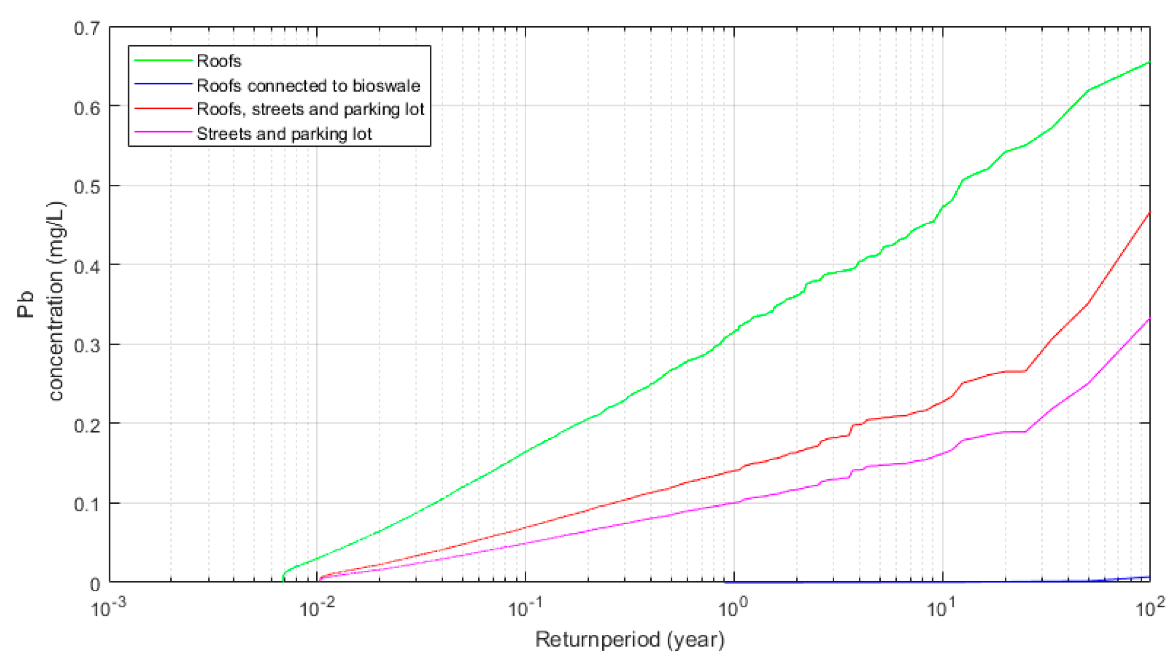
The tool returns the volumes of overflow, infiltration, and reuse or throughput water. The expected concentrations for different pollutants are also shown. The concentrations from different surface types in the project can be compared. The impact of different SUDS types can also be evaluated. An example of the output is shown in Figure 3.
2.2. Sampling Campaigns
The model for urban runoff pollution was validated by sampling campaigns in four separate sewer systems in Flanders, receiving storm water from small catchments. Details about the catchments are given in Table 1. A map showing the locations of the catchments is given in Figure A1, Figure A2, Figure A3 and Figure A4.
In the catchments Wilsele and Walem, samples were collected during different storm events by automatic samplers in a sewer manhole, where each sample was an average of samples taken every five minutes. In Wolvenberg and Mechelen, grab samples were collected manually in a sewer manhole during a few storm events.
All samples were cooled to 4 °C and analyzed using the standard methods in Table 2 for Zn, Cu, Pb, TSS, TN, and TP.
No rain gauges were available at the measurement sites, so the data of the closest public rain gauge [38] were used. The rainfall characteristics of the sampled storms are shown in Table A1. The building types were determined from Google Maps images.
To compare the model results with the samples, the average concentration for each storm event was calculated. As the catchments are small, it was assumed that no transformation of pollutants in the sewer pipe takes place. This could result in an overestimation of the sample concentrations.
3. Results
Table 3 shows the average concentrations measured in the four catchments. Clear differences between the catchments are apparent. The highest concentrations are found in the Wolvenberg catchment, which consists of a medium trafficked road. The heavy metal concentrations in the Walem catchment are also significantly higher than in the Mechelen and Wilsele catchments. For TN and TP, the concentrations vary less between the different catchments.
The measurements were compared with the StormTac database [14], which collects pollutant concentrations found in a large number of international storm water sampling campaigns and reports standard values for different types of land use.
The Wolvenberg catchment consists of a medium trafficked road with an average daily traffic (ADT) of 6500 vehicles and can be compared with road type 5 (ADT of 10,000) in the StormTac database. Nevertheless, the pollutant concentrations in Wolvenberg are significantly higher than in the database. Furthermore, the catchments Mechelen, Walem, and Wilsele can all be classified as residential or downtown areas, so the StormTac database is not able to explain the higher heavy metal concentrations in the Walem catchment.
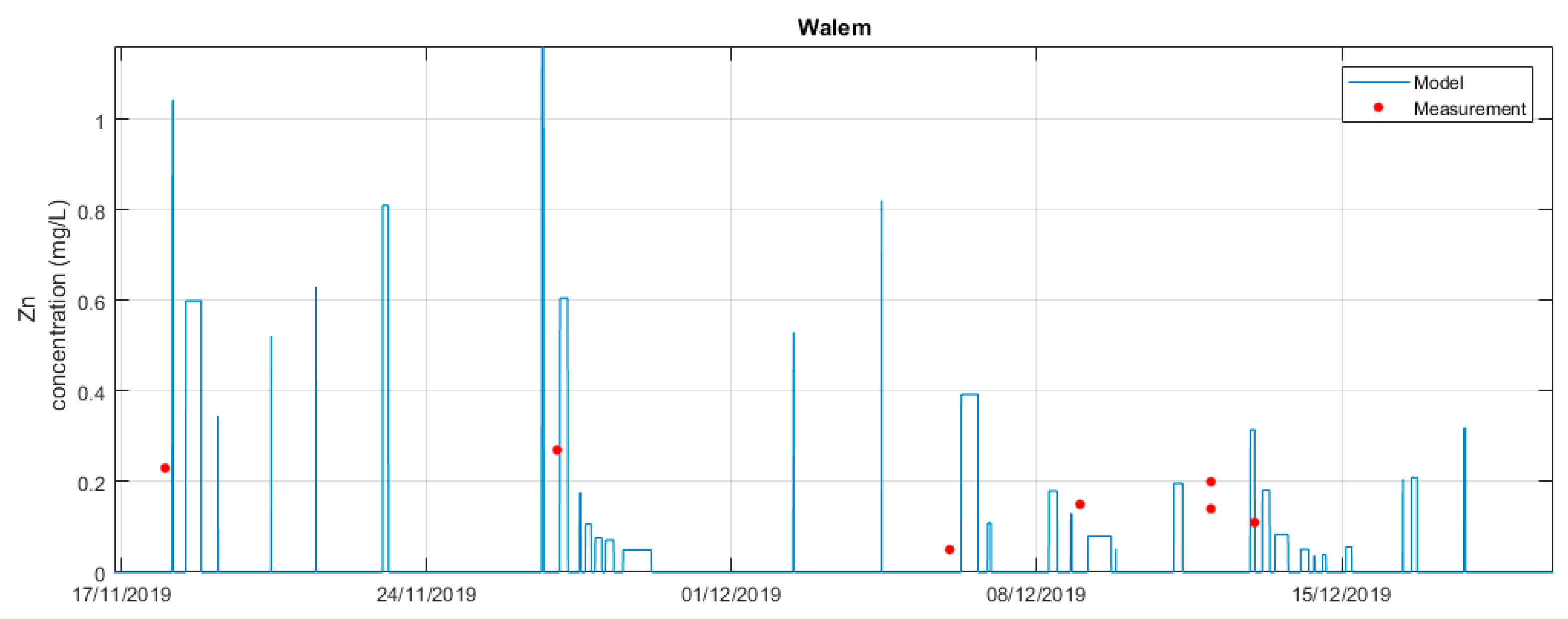
In Figure 4, Figure 5 and Figure 6, modelled concentrations (Equation (3)) are compared with measurements in four small Flemish catchments.
Figure 4 shows a part of the time series of the zinc concentration in the catchment Walem. As the rain gauge that was used as input for the model was 6.2 km away from the sampling location, the peaks of the rain events in the model do not always coincide with the sampled events.
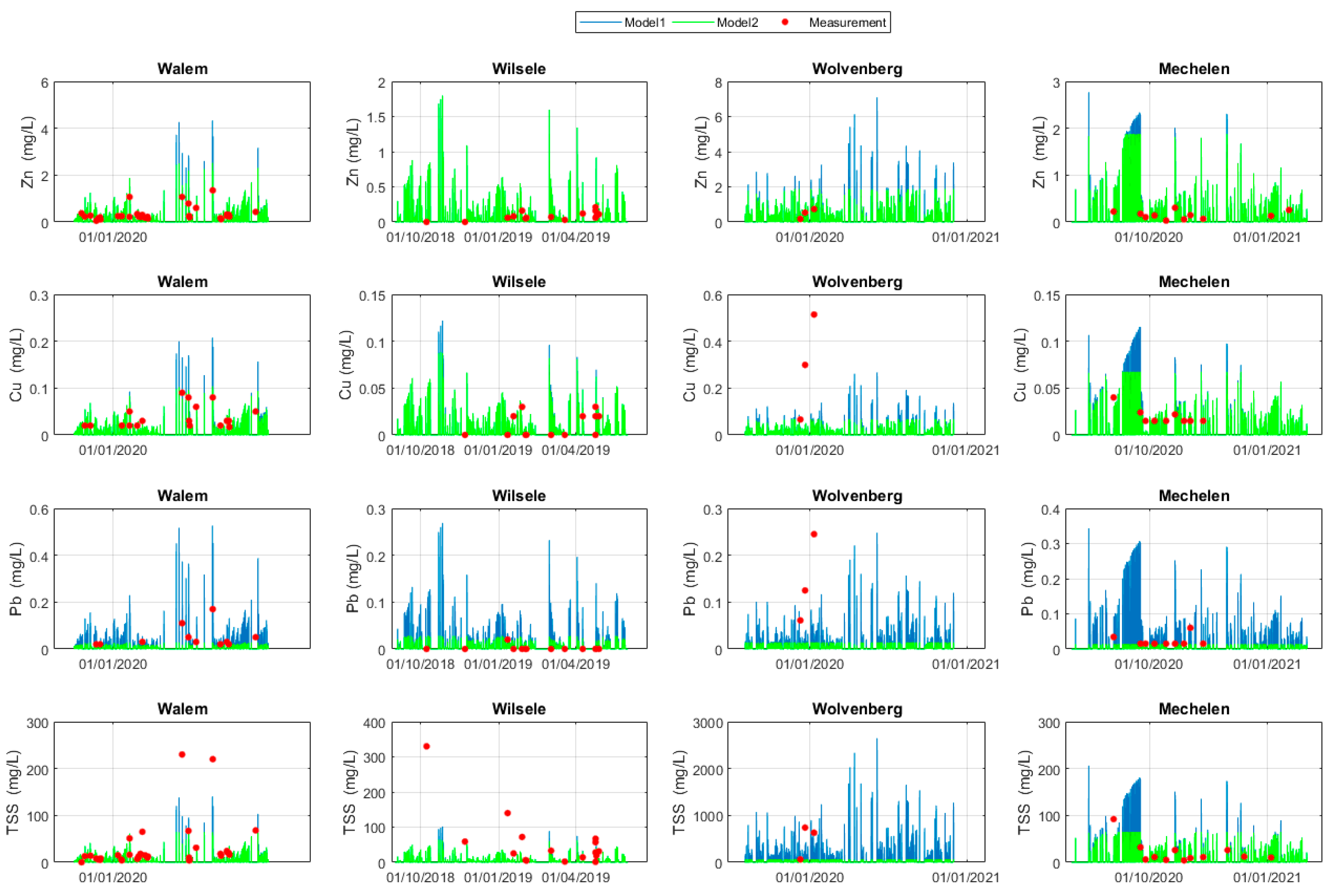
Figure 5 compares the measured and modeled heavy metal and TSS concentrations for all catchments (model 2 vs. measurement). For reasons of comparison, the model results without the maximum pollutant build-up value are also shown (model 1).
Overall, the model is able to reproduce the spread in concentrations and the differences between the catchments. There is a clear improvement compared to the use of a database with standard concentrations. The model correctly predicts larger heavy metal concentrations in the Walem catchment than in Wilsele and Mechelen, even though the catchments are very similar. For the catchment Wolvenberg, the modeled Cu and Pb concentrations are too low, but they are in the same order of the StormTac database. This is not related to the maximum build-up value, as the curves for model 1 and model 2 are very similar. For Wilsele, too, the results for Pb and Cu are poor. Here, the concentrations are close to the detection limits, which explains the large number of samples with zero concentration and the poor model performance. For Zn and Cu, the maximum build-up value slightly improved the model results but did not have much impact. For Pb and TSS, the maximum build-up value seems to underestimate the measured concentrations.
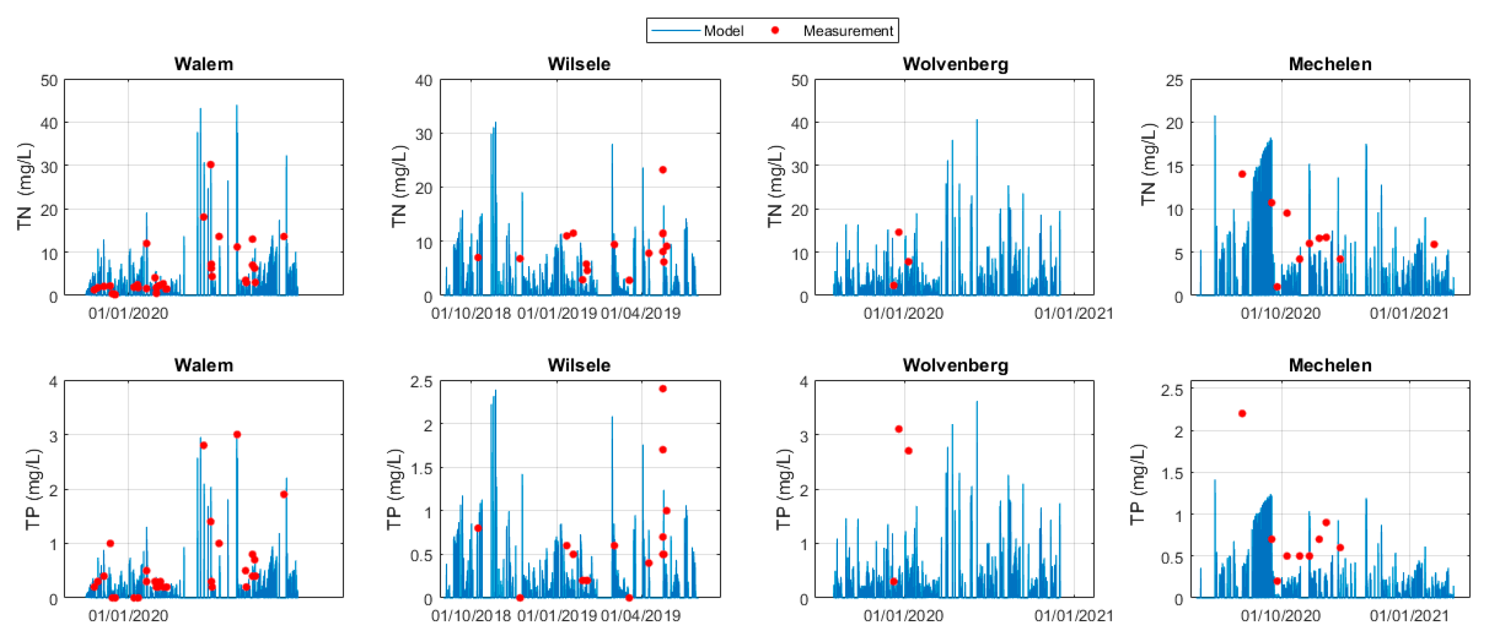
For TP and TN, no maximum build-up values were used. Nevertheless, the modeled results compare well with the measurements (Figure 6).
4. Discussion
A common approach to assessing the impact of urban runoff is to use average pollutant concentrations based on the type of land use. These concentrations are collected in databases such as StormTac. The first difficulty with this approach is finding the land use that fits best with the study area. For the Wolvenberg catchment, this is straightforward, as it consists of a single medium trafficked road section, with no roofs connected. Nevertheless, the observed concentrations are significantly higher than the ones in the database. Next to the surface type and traffic volume, rainfall characteristics also influence the pollutant concentrations, and these are not taken into account when average concentrations are used.
For the other catchments in this work, the land use fits best with a residential area. The concentrations in StormTac for this land use are indeed in the same order of magnitude as in this study. However, the database does not take into account differences in population density or building types, so the same concentrations for all residential areas are reported. Nevertheless, in this study, we found significantly higher heavy metal concentrations in the Walem catchment compared to Wilsele and Mechelen. There are some databases that differentiate residential areas based on their building density, such as USEPA. Still, this could not explain the observed differences, as the three residential areas in this study have comparable building densities (Table 1).
Furthermore, the use of average concentrations fails to predict the conditions under which peak concentrations are emitted, which is important in assessing ecotoxicity on surface waters.
The runoff model developed in this work tackles the issues described above, as (1) it turns loads into concentrations using local rainfall data that reproduces the time variation of the concentrations, and (2) it uses detailed site-specific information such as the exact location (atmospheric deposition), building types, building density, and traffic volume, which allows for better discernment between similar catchments. Another advantage of our model is that it does not need to be calibrated, contrary to the build-up/wash-off models that are also commonly used in other tools.
As expected, the aquaSens model was not capable of accurately reproducing the measured pollutant concentrations. In particular, the maximum build-up values still need to be better established, which may improve the performance of the model. However, the spread in the concentrations during different storm events was overall well reproduced. There is a clear improvement compared to a modeling approach with a constant average concentration. Furthermore, the model was able to reproduce the differences between the catchments, even though they are quite similar.
The model shows that the high TSS and Zn concentrations in Wolvenberg originate mainly from traffic emissions. The aquaSens runoff model approaches these concentrations much more closely than the stormTac database.
Although Wilsele, Walem, and Mechelen are all residential areas with a similar building density, the heavy metal concentrations are significantly higher in the Walem catchment, especially for Zn. Our model correctly predicts the higher concentrations in Walem. The heavy metals mainly originate from rooftops. The building types in Walem are different from the other catchments. A school and industrial building contribute to the higher concentrations. The contribution from atmospheric distribution is also larger in Walem than in Mechelen and Wilsele.
Note that the transformation of pollutants in the sewer systems, e.g., due to sedimentation, was not taken into account in the model. Perhaps the emission factors are somewhat underestimated, which compensates for the effect of sedimentation. The catchments are small, so the effect of sedimentation will still be limited. Further research is necessary to verify the ways in which this affects the concentrations in larger catchments.
5. Conclusions
In the current work, a new tool to model the concentration of different pollutants in urban runoff was presented. The model succeeds at explaining the time dependency of concentrations in urban runoff, which is a clear advantage compared to the common approach of using average land use-dependent concentrations. Furthermore, the model also predicted the higher heavy metal concentrations observed in the Walem residential area compared to two others residential areas, which could be attributed to different building types.
Given the promising results, the runoff quality model can be used by decision makers to assess the surfaces in a catchment that are in need of treatment before discharge to the receiving waters. One strategy could be to keep the most polluted surfaces connected to the combined sewer system and only discharge cleaner surfaces through separate sewer systems. Alternatively, runoff from polluted surfaces can be treated by SUDS or other stormwater treatment systems. The aquaSens tool can be used to determine the optimum SUDS type, and the dimensions of these systems are necessary to improve the water quality to predefined standards.
Figure 3 shows an example of the calculated runoff Pb concentration from a small catchment with one street, a parking lot, and 22 buildings. The model counterintuitively predicts that the runoff from the roofs is more polluted then the runoff from the road and parking lot, because there is not much traffic on the road. This example shows the need for a model-based approach. The Belgian groundwater environmental standard for lead amounts is 0.02 mg/L, which is frequently exceeded in this catchment for all surfaces. By connecting the roofs to a bioswale, a large part of the stormwater is infiltrated, which drastically improves the quality of overflow water, thereby protecting receiving waters.
Future research is needed to check whether the runoff quality model can also be used for larger catchments and whether it is applicable for estimating the concentrations of PAHs. Other emerging pollutants, such as PFAS, microplastics, or pesticides can also be included.
The SUDS model will be further elaborated and validated in future work. More SUDS types, such as sand filters or adsorption materials, will also be incorporated into the tool.
Author Contributions
Conceptualization, E.V. and E.L.; Methodology, E.V. and B.D.B.; Software E.V. and T.W.; Validation, E.V.; Formal Analysis, E.V.; Resources, E.V.; Writing—Original Draft Preparation, E.V.; Writing—Review and Editing: B.D.B., T.W. and R.D. All authors have read and agreed to the published version of the manuscript.
Funding
This research received no external funding.
Data Availability Statement
Data are contained within the article.
Acknowledgments
The authors wish to thank Idzi Hubrecht and Jurgen Meirlaen for explaining the WEISS tool.
Conflicts of Interest
The authors declare no conflict of interest.
Abbreviations
| ADT | Average daily traffic |
| RSS | Risk assessment of road stormwater runoff |
| SUDS | Sustainable urban drainage systems |
Appendix A
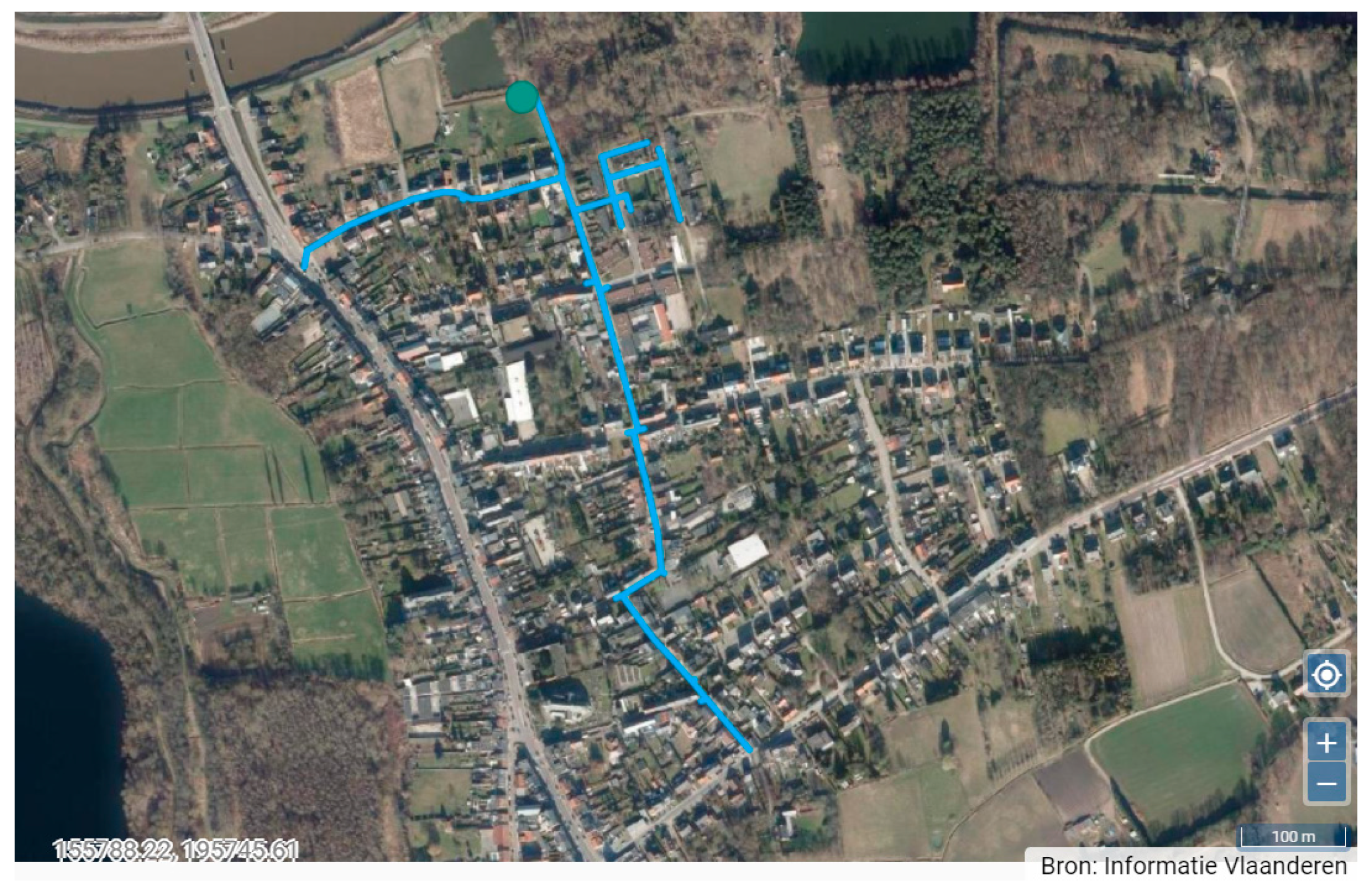
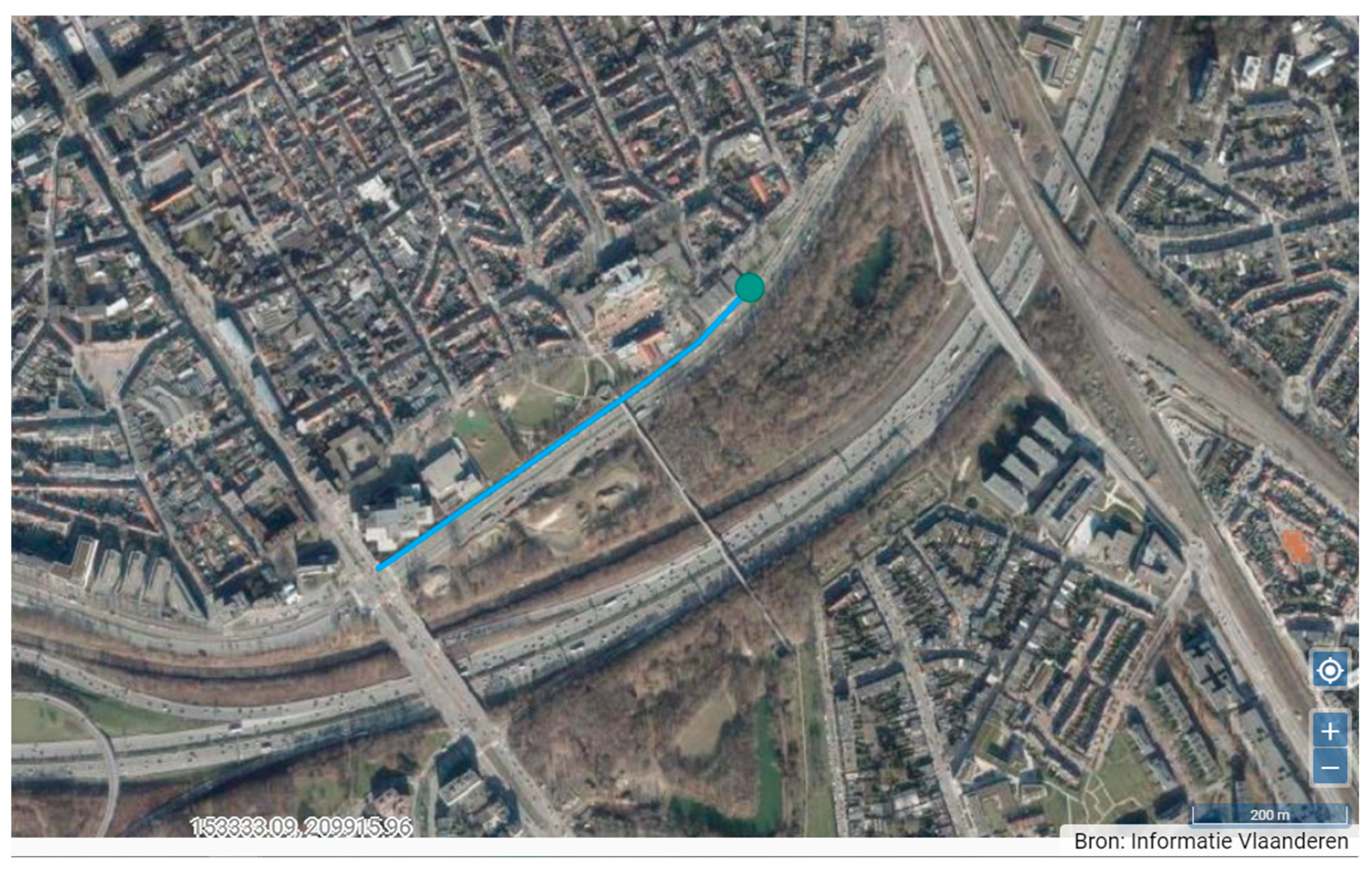
Figure A1.
Overview of the catchment in Wilsele. The green dot shows the inspection well where the samples were taken. The blue area is connected to this inspection well.
Figure A1.
Overview of the catchment in Wilsele. The green dot shows the inspection well where the samples were taken. The blue area is connected to this inspection well.

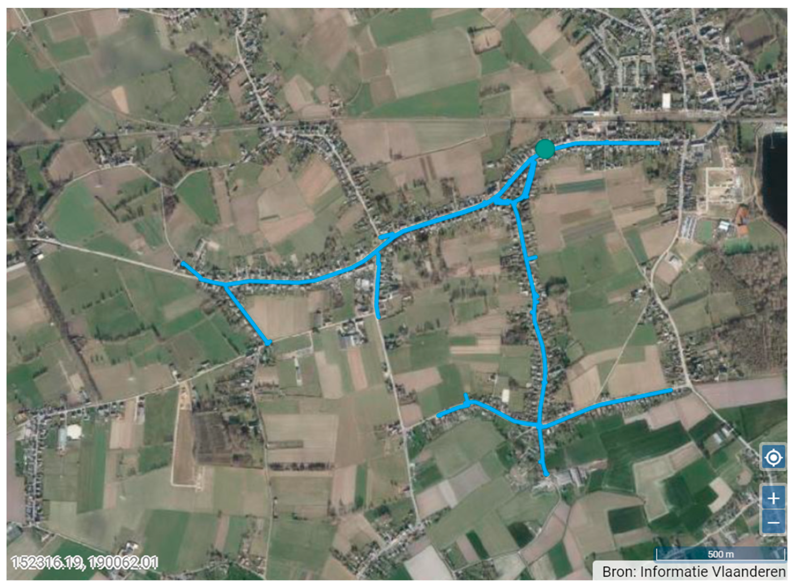
Figure A2.
Overview of the catchment in Wilsele. The green dot shows the inspection well where the samples were taken. The blue area is connected to the inspection well.
Figure A2.
Overview of the catchment in Wilsele. The green dot shows the inspection well where the samples were taken. The blue area is connected to the inspection well.

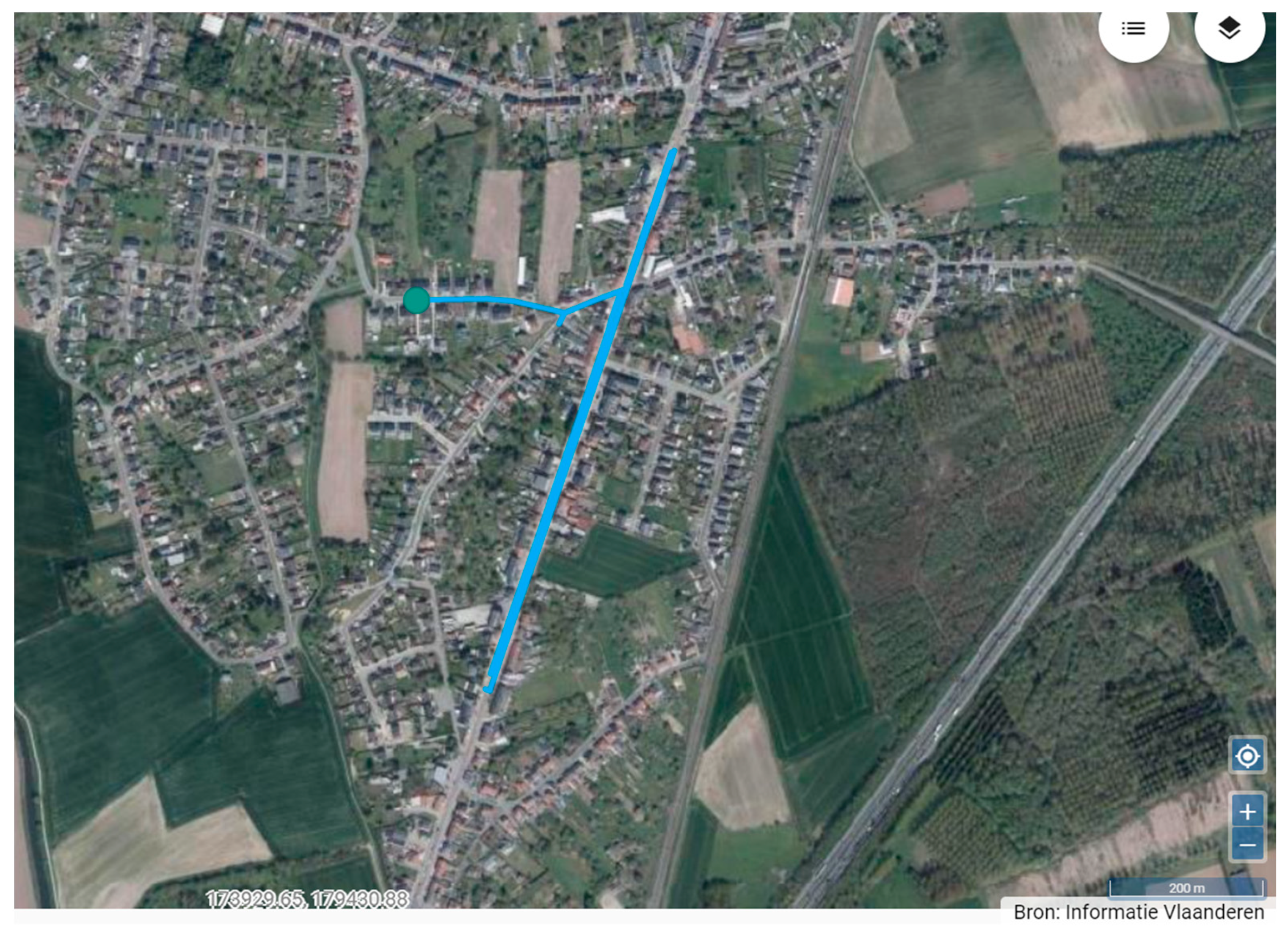
Figure A3.
Overview of the catchment in Wolvenberg. The green dot shows the inspection well where the samples were taken. The blue area is connected to this inspection well.
Figure A3.
Overview of the catchment in Wolvenberg. The green dot shows the inspection well where the samples were taken. The blue area is connected to this inspection well.

Figure A4.
Overview of the catchment in Mechelen. The green dot shows the inspection well where the samples were taken. The blue area is connected to this inspection well.
Figure A4.
Overview of the catchment in Mechelen. The green dot shows the inspection well where the samples were taken. The blue area is connected to this inspection well.

Appendix B

Table A1.
Rainfall characteristics of storms during sampling period. The resolution of the rain gauge was 1 min.
Table A1.
Rainfall characteristics of storms during sampling period. The resolution of the rain gauge was 1 min.
| Catchment | Storm Duration (h) | Mean Storm Intensity (mm/h) | Maximum Storm Intensity (mm/h) |
|---|---|---|---|
| Walem | 0–6.9 | 0.4–13.5 | 3.0–40.0 |
| Wilsele | 0–10.7 | 0.4–7.6 | 3.0–28.8 |
| Wolvenberg | 0–2.1 | 1.0–1.3 | 2.4–6.6 |
| Mechelen | 0–3.7 | 0.4–6.4 | 3.0–15.0 |
Appendix C
Table A2.
Emission factors for buildings (g/building/year) in WEISS.
| After 1970 | Before 1970 | |||||||
|---|---|---|---|---|---|---|---|---|
| Type of Building | Zn | Cu | Pb | Al | Zn | Cu | Pb | Al |
| Attached buildings | 21 | 1.36 | 3.6 | 0.007 | 26.5 | 1.54 | 4.361 | 0 |
| Semi-detached buildings | 19.3 | 1.33 | 3.6 | 0.009 | 39.6 | 1.81 | 4.388 | 0 |
| Detached building | 27.9 | 2.34 | 4.05 | 0.005 | 57.8 | 2.55 | 4.219 | 0 |
| Apartments | 164.521 | 1.843 | 1.52 | 0.019 | 241.89 | 1.928 | 0.048 | 0 |
| Side buildings | 8.8 | 0 | 0.63 | 0.016 | 14.61 | 0 | 0.68 | 0 |
| Offices | 164.521 | 1.843 | 1.52 | 0.019 | 241.89 | 1.928 | 0.048 | 0 |
| Industrial buildings | 260.622 | 0 | 17.64 | 6.879 | 720.245 | 0 | 31.752 | 6.882 |
| Commercial buildings | 27.9 | 2.34 | 4.05 | 0.005 | 57.8 | 2.55 | 4.219 | 0 |
| All ages | ||||||||
| Schools | 548.38 | 11.115 | 6 | 0.22 | ||||
| Churches | 118.319 | 75.51 | 0 | 0 | ||||
| Sports centers | 46.913 | 0 | 0 | 0 | ||||
| Stations | 136.13 | 0 | 1.375 | 0 | ||||
Table A3.
Emission factors for vehicles (g/million vehicle km) in WEISS.
| Source | Road Type | Voertuig | Zn | Cu | Pb | PAK16 |
|---|---|---|---|---|---|---|
| tyre wear | highway | van | 272 | 14 | 4.6 | 15.713 |
| tyre wear | highway | bus | 1051 | 54 | 18 | 40.402 |
| tyre wear | highway | motor | 417 | 21 | 7 | 5.613 |
| tyre wear | highway | passenger car | 190 | 9.8 | 3.2 | 11.226 |
| tyre wear | highway | special vehicle | 3990 | 205 | 67 | 41.525 |
| tyre wear | highway | truck | 1921 | 99 | 32 | 47.3172 |
| tyre wear | municipal road | van | 1631 | 84 | 27 | 31.424 |
| tyre wear | municipal road | bus | 7830 | 402 | 131 | 50.8003 |
| tyre wear | municipal road | motor | 417 | 21 | 7 | 11.226 |
| tyre wear | municipal road | passenger car | 1124 | 58 | 19 | 22.446 |
| tyre wear | municipal road | special vehicle | 2660 | 137 | 45 | 53.0483 |
| tyre wear | municipal road | truck | 14,350 | 737 | 241 | 64.6677 |
| tyre wear | regional road | van | 816 | 42 | 14 | 15.713 |
| tyre wear | regional road | bus | 3371 | 173 | 57 | 40.402 |
| tyre wear | regional road | motor | 417 | 21 | 7 | 5.613 |
| tyre wear | regional road | passenger car | 653 | 34 | 11 | 11.226 |
| tyre wear | regional road | special vehicle | 2660 | 137 | 45 | 41.525 |
| tyre wear | regional road | truck | 5347 | 275 | 90 | 47.3352 |
| wegdekslijtage | highway | van | 9.5 | 3.2 | 4.1 | 3.125 |
| road wear | highway | bus | 28 | 9.7 | 12 | 15.918 |
| road wear | highway | motor | 3.6 | 1.2 | 1.6 | 2.55 |
| road wear | highway | passenger car | 7.2 | 2.5 | 3.1 | 6.25 |
| road wear | highway | special vehicle | 34 | 12 | 14 | 19.042 |
| road wear | highway | truck | 39 | 13 | 17 | 15.918 |
| road wear | municipal road | van | 6.3 | 2.2 | 2.7 | 28.368 |
| road wear | municipal road | bus | 19 | 6.5 | 8.1 | 95.1155 |
| road wear | municipal road | motor | 2.4 | 0.83 | 1 | 11.608 |
| road wear | municipal road | passenger car | 4.8 | 1.7 | 2.1 | 28.368 |
| road wear | municipal road | special vehicle | 22 | 7.7 | 9.6 | 54.5443 |
| road wear | municipal road | truck | 26 | 8.9 | 11 | 95.1155 |
| road wear | regional road | van | 6.3 | 2.2 | 2.7 | 6.25 |
| road wear | regional road | bus | 19 | 6.5 | 8.1 | 31.835 |
| road wear | regional road | motor | 2.4 | 0.83 | 1 | 2.55 |
| road wear | regional road | passenger car | 4.8 | 1.7 | 2.1 | 6.249 |
| road wear | regional road | special vehicle | 22 | 7.7 | 9.6 | 19.042 |
| road wear | regional road | truck | 26 | 8.9 | 11 | 31.837 |
| leakage engine | highway | van | 183 | 2.6 | 2.5 | 8.1001 |
| leakage engine | highway | bus | 301 | 4.2 | 4.2 | 8.1001 |
| leakage engine | highway | motor | 8.1001 | |||
| leakage engine | highway | passenger car | 183 | 2.6 | 2.5 | 8.1001 |
| leakage engine | highway | special vehicle | 301 | 4.2 | 4.2 | 8.1001 |
| leakage engine | highway | truck | 301 | 4.2 | 4.2 | 8.1001 |
| leakage engine | municipal road | van | 183 | 2.6 | 2.5 | 32.4004 |
| leakage engine | municipal road | bus | 301 | 4.2 | 4.2 | 32.4004 |
| leakage engine | municipal road | motor | 32.4004 | |||
| leakage engine | municipal road | passenger car | 183 | 2.6 | 2.5 | 32.4004 |
| leakage engine | municipal road | special vehicle | 301 | 4.2 | 4.2 | 32.4004 |
| leakage engine | municipal road | truck | 301 | 4.2 | 4.2 | 32.4004 |
| leakage engine | regional road | van | 183 | 2.6 | 2.5 | 8.1001 |
| leakage engine | regional road | bus | 301 | 4.2 | 4.2 | 8.1001 |
| leakage engine | regional road | motor | 8.1001 | |||
| leakage engine | regional road | passenger car | 183 | 2.6 | 2.5 | 8.1001 |
| leakage engine | regional road | special vehicle | 301 | 4.2 | 4.2 | 8.1001 |
| leakage engine | regional road | truck | 301 | 4.2 | 4.2 | 8.1001 |
Table A4.
Emission factors for TN and TP, taken from reference [36].
Table A4.
Emission factors for TN and TP, taken from reference [36].
| Source | N (kg/ha/Year) | P (kg/ha/Year) |
|---|---|---|
| Atmospheric deposition (wet + dry) | 11 | 0.47 |
| Leaf fall | 3.2 | 0.32 |
| Erosion sand and soil | 0 | 0.08 |
| Urine and fecal matter from pets | 3.9 | 0.74 |
| Urine and fecal matter from birds | 0.045 | 0.015 |
| Total | 18 | 1.6 |
Table A5.
Maximum build-up values and wash-off rates for different pollutants, taken from reference [13].
Table A5.
Maximum build-up values and wash-off rates for different pollutants, taken from reference [13].
| Pollutant | Maximum Build Up (mg/m2) | Wash-Off Rate (−) |
|---|---|---|
| Zn | 4.7 | 0.32 |
| Cu | 0.27 | 0.20 |
| Pb | 0.039 | 0.29 |
| TSS | 173 | 0.24 |
| Other | Inf | 0.3 |
References
- Sartor, J.D.; Boyd, G.B. Water Pollution Aspects of Street Surface Contaminants; EPA-R2-72-081; US Environmental Protection Agency: Washington, DC, USA, 1972.
- Lee, H.; Swamikannu, X.; Radulescu, D.; Kim, S.; Stenstrom, M.K. Design of stormwater monitoring programs. Water Res. 2007, 41, 4186–4196. [Google Scholar] [CrossRef] [PubMed]
- Björklund, K.; Bondelind, M.; Karlsson, A.; Karlsson, D.; Sokolova, E. Hydrodynamic modelling of the influence of stormwater and combined sewer overflows on receiving water quality: Benzo(a)pyrene and copper risks to recreational water. J. Environ. Manag. 2018, 207, 32–42. [Google Scholar] [CrossRef] [PubMed] [Green Version]
- Müller, A.; Österlund, H.; Marsalek, J.; Viklander, M. The pollution conveyed by urban runoff: A review of sources. Sci. Total Environ. 2020, 709, 13612. [Google Scholar] [CrossRef] [PubMed]
- Zhou, Q. A review of sustainable urban drainage systems considering the climate change and urbanization impacts. Water 2014, 6, 976–992. [Google Scholar] [CrossRef] [Green Version]
- Jayasooriya, V.M.; Ng, A.W.M. Tools for Modeling of Stormwater Management and Economics of Green Infrastructure Practices: A Review. Water Air Soil Pollut. 2014, 225, 2055. [Google Scholar] [CrossRef] [Green Version]
- Bonhomme, C.; Petrucci, G. Should we trust build-up/wash-off water quality models at the scale of urban catchments? Water Res. 2017, 108, 422–431. [Google Scholar] [CrossRef]
- Egodawatta, P.; Goonetilleke, A. Characteristics of pollutants build-up on residential road surfaces. In Proceedings of the 7th International Conference on Hydroscience and Engineering, Philadelphia, PN, USA, 10–13 September 2006. [Google Scholar]
- Egodawatta, P. Translation of Small-Plot Scale Pollutant Build-Up and Wash-Off Measurements to Urban Catchment Scales; Faculty of Built Environment and Engineering, Queensland University of Technology: Brisbane City, Australia, 2007. [Google Scholar]
- Egodawatta, P.; Thomas, E.; Goonetilleke, A. Understanding the physical processes of pollutant build-up and wash-off on roof surfaces. Sci. Total Environ. 2009, 407, 1834–1841. [Google Scholar] [CrossRef] [PubMed] [Green Version]
- Liu, A.; Liu, L.; Li, D.; Guan, Y. Characterizing heavy metal build-up on urban road surfaces: Implication for stormwater reuse. Sci. Total Environ. 2015, 515–516, 20–29. [Google Scholar] [CrossRef] [PubMed]
- Hossain, I.; Imteaz, M.; Gato-Trinidad, S.; Shanableh, A. Development of a Catchment Water Quality Model for Continuous Simulations of Pollutants Build-up and Wash-off. Int. J. Environ. 2010, 4, 11–18. [Google Scholar]
- Wicke, D.; Cochrane, T.A.; O’Sullivan, O. Build-up dynamics of heavy metals deposited on impermeable urban surfaces. J. Environ. 2012, 113, 347–354. [Google Scholar] [CrossRef] [PubMed]
- StormTac Database. Stormwater, Baseflow, Surface Water and Wastewater Database, V.2022-10-27; StormTac Corporation: Stockholm, Sweden, 2022; Available online: www.stormtac.com (accessed on 15 January 2023).
- Gardinera, L.R.; Mooresb, J.; Osbornea, A.; Semadeni-Daviesb, A. Risk assessment of road stormwater runoff. In NZ Transport Agency Research Report; Australian Road Research Board (ARRB): Melbourne, Australia, 2016; Volume 585. Available online: https://www.nzta.govt.nz/assets/resources/research/reports/585/585-risk-assessment-of-road-stormwater-runoff.pdf (accessed on 15 January 2023).
- Common Implementation Strategy for the Water Framework Directive (2000/60/EC); Guidance Document No. 28; European Commission: Brussels, Belgium, 2012.
- WEISS Geoloket. Available online: https://weissgeoloket.marvin.vito.be/source (accessed on 15 January 2023).
- Van Esch, L.; Vos, G.; Janssen, L.; Engelen, G. The Emission Inventory Water: A Planning Support System for Reducing Pollution Emissions in the Surface Waters of Flanders. In Planning Support Systems Best Practice and New Methods; Geertman, S., Stillwell, J., Eds.; Springer: Berlin/Heidelberg, Germany, 2009; Volume 95, 490p. [Google Scholar]
- Van Esch, L.; Uljee, I.; Engelen, G.; Vos, G.; Hermans, G. The Water Emission Inventory planning Support System (WEISS): A quantification of environmental pressures following the path from the emission source to the surface water. In Proceedings of the International Congress on Environmental Modelling and Software Managing Resources of a Limited Planet, Leipzig, Germany, 1–5 July 2012. [Google Scholar]
- Willems, P. Compound IDF-relationships of extreme precipitation for two seasons and two storm types. J. Hydrol. 2000, 233, 189–205. [Google Scholar] [CrossRef]
- Engelen, G.; Van Esch, L. Evolutie van de Emissies in Water uit Corrosie van Bouwmaterialen aan de Hand van de Referentiejaren 1998, 2002 en 2005. Report 2007/IMS/R428 VITO, Mol. 2007. Available online: https://archief-algemeen.omgeving.vlaanderen.be/xmlui/handle/acd/762021 (accessed on 15 January 2023).
- Oosterhuis, M.; Korenromp, R.H.J. Verontreiniging van de Infiltratievoorziening. TNO Rapport R 2002/618. Available online: http://essay.utwente.nl/56954/1/Scriptie_van_Rens.pdf (accessed on 15 January 2023).
- van Rens, C.P.M. Zuiveren van Afstromend Regenwater? Beslismodel ter Ondersteuning van Keuze voor Bronmaatregelen en ‘End of Pipe’-Voorzieningen. Master’s Thesis, Universiteit Twente, Twente, The Netherlands, 2006. [Google Scholar]
- Brodie, I. Suspended Solids in Stormwater Runoff from Various Urban Surfaces; Report to Condamine Alliance; USQ: Darling Heights, Australia, 2005. [Google Scholar]
- Charters, F.J.; Cochrane, T.A.; O’Sullivan, A.D. Untreated runoff quality from roof and road surfaces in a low intensity rainfall climate. Sci. Total Environ. 2016, 550, 265–272. [Google Scholar] [CrossRef] [PubMed]
- De Buyck, P.J.; Van Hulle, S.W.H.; Dumoulin, A.; Rousseau, D.P.L. Roof runoff contamination: A review on pollutant nature, material leaching and deposition. Rev. Environ. Sci. Biotechnol. 2021, 20, 549–606. [Google Scholar] [CrossRef]
- Brown, J.N.; Peake, B.M. Sources of heavy metals and polycyclic aromatic hydrocarbons in urban stormwater runoff. Sci. Total Environ. 2006, 359, 145–155. [Google Scholar] [CrossRef] [PubMed]
- Lamprea, K.; Ruban, V. Characterization of atmospheric deposition and runoff water in a small suburban catchment. Environ. Technol. 2011, 32, 1141–1149. [Google Scholar] [CrossRef] [PubMed]
- Petrucci, G.; Gromaire, M.-C.; Shorshani, M.F.; Chebbo, G. Nonpoint source pollution of urban stormwater runoff: A methodology for source analysis. Environ. Sci. Pollut. Res. 2014, 21, 10225–10242. [Google Scholar] [CrossRef] [PubMed]
- Ali, S.A.; Debade, X.; Chebbo, G. Contribution of atmospheric dry deposition to stormwater loads for PAHs and trace metals in a small and highly trafficked urban road catchment. Environ. Sci. Pollut. Res. 2017, 24, 26497–26512. [Google Scholar] [CrossRef] [PubMed]
- Deltares, T. Emissieschattingen Diffuse Bronnen Emissieregistratie; Tyre Wear Wegverkeer; Rijkswaterstaat–WVL: Utrecht, The Netherlands, 2016. [Google Scholar]
- Baensch-Baltruschat, B.; Kocher, B.; Kochleus, C.; Stock, F.; Reifferscheid, G. Tyre and road wear particles—A calculation of generation, transport and release to water and soil with special regard to German roads. Sci. Total Environ. 2021, 752, 141939. [Google Scholar] [CrossRef] [PubMed]
- US EPA Nationwide Urban Runoff Program (NURP). 1983. Available online: https://www3.epa.gov/npdes/pubs// (accessed on 15 January 2023).
- Partners4Water. Afstroming van N en P. Internal Report. 2018. Available online: https://legacy.emissieregistratie.nl/erpubliek/documenten/06%20Water/01%20Factsheets/02%20Achtergronddocumenten%20bij%20de%20factsheets/P4UW_Achtergrondrapport_afspoeling_N_en_P_2018.pdf (accessed on 15 January 2023).
- Rietveld, M.; Clemens, F.; Langeveld, J. Solids dynamics in gully pots. Urban Water J. 2020, 17, 669–680. [Google Scholar] [CrossRef]
- Boogaard, F.C.; van de Ven, F.; Langeveld, J.G.; Kluck, J.; van de Giesen, N. Removal efficiency of storm water treatment techniques: Standardized full scale laboratory testing. Urban Water J. 2015, 14, 255–262. [Google Scholar] [CrossRef]
- Straatvinken. Available online: http://straatvinken.datylon.com/ (accessed on 15 January 2023).
- Waterinfo. Available online: www.waterinfo.be (accessed on 15 January 2023).
Figure 1.
Pollutant sources in the aquaSens tool.

Figure 2.
Scheme of the build-up/wash-off model.

Figure 3.
Example of the output of the aquaSens tool for the lead concentration in runoff water for a catchment with roofs, a street, and a parking lot.
Figure 3.
Example of the output of the aquaSens tool for the lead concentration in runoff water for a catchment with roofs, a street, and a parking lot.

Figure 4.
Detail of the modelled Zn concentrations in Walem.

Figure 5.
Modeled and measured heavy metals and TSS concentrations in different catchments. Model1 shows the concentrations derived by the WEISS method, without assuming a maximum build up, whereas in model 2, a maximum build up is incorporated.
Figure 5.
Modeled and measured heavy metals and TSS concentrations in different catchments. Model1 shows the concentrations derived by the WEISS method, without assuming a maximum build up, whereas in model 2, a maximum build up is incorporated.

Figure 6.
Modeled and measured TP and TN concentrations in different catchments.

Table 1.
Details of the catchments.
| Catchment Name | Road Area (m2) | Roof Area (m2) | Nr Buildings (/ha) | Traffic Volume (/u) 1 | Nr of Samples | Distance to Rain Gauge (km) |
|---|---|---|---|---|---|---|
| Walem | 3780 | 7880 | 53.9 | 30 | 34 | 6.2 |
| Wilsele | 27,000 | 26,000 | 100.0 | 105 | 15 | 5.9 |
| Wolvenberg | 5600 | 0 | 0 | 270 | 3 | 6.7 |
| Mechelen | 29,210 | 61,980 | 71.8 | 79 | 13 | 6.3 |
Note: 1 Data taken from the results of a citizen science project [37].
Table 2.
Analytical methods.
| Pollutant | Analytical Method |
|---|---|
| Zn | WAC/III/B/002 (digestion HNO3/HCl)–WAC/III/B/010 (ICP-AES) |
| Cu | WAC/III/B/002 (digestion HNO3/HCl)–WAC/III/B/010 (ICP-AES) |
| Pb | WAC/III/B/002 (digestion HNO3/HCl)–WAC/III/B/010 (ICP-AES) |
| TSS | WAC/III/D/002 (gravimetric) |
Table 3.
Average pollutant concentrations in the four catchments, compared with average concentrations in the StormTac database [14].
Table 3.
Average pollutant concentrations in the four catchments, compared with average concentrations in the StormTac database [14].
| Catchment Name | Zn (mg/L) | Cu (mg/L) | Pb (mg/L) | TSS (mg/L) | TN (mg/L) | TP (mg/L) |
|---|---|---|---|---|---|---|
| Walem | 0.34 | 0.04 | 0.05 | 30.94 | 5.30 | 0.66 |
| Wilsele | 0.08 | 0.02 | <0.02 | 55.58 | 8.69 | 0.74 |
| Wolvenberg | 0.48 | 0.29 | 0.14 | 477.00 | 8.23 | 2.03 |
| Mechelen | 0.15 | 0.02 | 0.02 | 20.33 | 6.88 | 1.50 |
| StormTac Road 5 | 0.14 | 0.032 | 0.014 | 81 | 1.8 | 0.15 |
| StormTac Residential Area * | 0.11 | 0.028 | 0.016 | 76 | 1.8 | 0.25 |
| StormTac downtown area | 0.16 | 0.032 | 0.018 | 100 | 1.9 | 0.29 |
Note: * indicates a lack of road ditches.
Disclaimer/Publisher’s Note: The statements, opinions and data contained in all publications are solely those of the individual author(s) and contributor(s) and not of MDPI and/or the editor(s). MDPI and/or the editor(s) disclaim responsibility for any injury to people or property resulting from any ideas, methods, instructions or products referred to in the content. |
© 2023 by the authors. Licensee MDPI, Basel, Switzerland. This article is an open access article distributed under the terms and conditions of the Creative Commons Attribution (CC BY) license (https://creativecommons.org/licenses/by/4.0/).
Share and Cite
MDPI and ACS Style
Vinck, E.; De Bock, B.; Wambecq, T.; Liekens, E.; Delgado, R. A New Decision Support Tool for Evaluating the Impact of Stormwater Management Systems on Urban Runoff Pollution. Water 2023, 15, 931. https://doi.org/10.3390/w15050931
AMA Style
Vinck E, De Bock B, Wambecq T, Liekens E, Delgado R. A New Decision Support Tool for Evaluating the Impact of Stormwater Management Systems on Urban Runoff Pollution. Water. 2023; 15(5):931. https://doi.org/10.3390/w15050931
Chicago/Turabian StyleVinck, Evi, Birgit De Bock, Tom Wambecq, Els Liekens, and Rosalia Delgado. 2023. "A New Decision Support Tool for Evaluating the Impact of Stormwater Management Systems on Urban Runoff Pollution" Water 15, no. 5: 931. https://doi.org/10.3390/w15050931
Note that from the first issue of 2016, this journal uses article numbers instead of page numbers. See further details here.