
Detection of the Bedload Movement with an Acoustic Sensor in the Yangtze River, China


1
School of River & Ocean Engineering, Chongqing Jiaotong University, Chongqing 400074, China
2
National Engineering Research Center for Inland Waterway Regulation, Chongqing Jiaotong University, Chongqing 400074, China
*
Author to whom correspondence should be addressed.
Water 2023, 15(5), 939; https://doi.org/10.3390/w15050939
Submission received: 29 December 2022
/
Revised: 16 February 2023
/
Accepted: 24 February 2023
/
Published: 28 February 2023
(This article belongs to the Section Soil and Water)
Abstract
:The acoustic method, which enables continuous monitoring with great temporal resolution, is an alternative technique for detecting bedload movement. In order to record the sound signals produced by the impacts between gravel particles and detect the bedload motion, in this study, a hydrophone is placed close to the riverbed at the upper Yangtze River. Three categories of raw audio signals—moving gravel particles, ship engines, and flow turbulence—are collected and investigated. Signal preprocessing is performed using spectral subtraction to reduce the noise of the background sound, and the sound signal characteristic parameters are then calculated. In this paper, we propose a novel method for detecting and extracting bedload motion parameters, including peak frequency, pitch frequency, and energy eigenvector. When a segment of a speech signal meets the indicators for all three feature parameters simultaneously, the segment signal is classified as a bedload motion sound signal. Further work will be conducted to investigate bedload transport using the extracted audio signal.
1. Introduction
Bedload transport is one of the basic problems in river dynamics for comprehending riverbed evolution, reservoir siltation, river regulation, and other issues [1]. The bedload movement appears to have obvious spatial and temporal variability and is even highly intermittent [2,3]. Bedload movement in mountain rivers has different transport characteristics, and there is mutual feedback and a complicated relationship between sediment transport characteristics and riverbed gradation, water, and sediment characteristics. Carrillo et al. [4] proposed a laboratory experimental model study to determine the bedload transport rate in steep channels. However, their study was limited to the flume scale. Kociuba [5] presented the effect of bedload transport on the development of an alluvial fan from a direct field measurement in a relatively small river.
The upper reaches of the Yangtze River are typical mountain rivers. As a result of cascade reservoir construction, which modifies downstream sediment movement and river flow, the initial natural equilibrium of the riverbed changed. These changes have a particularly large impact on navigation conditions, scouring and silting changes, and downstream channel-regulating measures. In addition to the bedload, suspended sediment transport can alter the riverbed, similar to that occurring in the ocean [6,7]. However, this study will focus on detecting gravel movement in the Yangtze River in order to assess the Yangtze River’s riverbed evolution mechanism.
In general, there are two types of bedload transport monitoring methods: direct measurement with samplers and indirect measurement by collecting relative physical parameters [8]. Bedload samplers [9,10] and sediment traps [11,12] are examples of direct methods. However, traditional bedload measurement techniques are only appropriate for a very limited range of hydraulic conditions because they are time consuming, expensive, and sometimes dangerous [13]. As a result, more effort has been invested in developing indirect bedload surrogate monitoring techniques over the last decade or so in order to overcome some of the limitations of the direct methods. The acoustic signal generated by the collision of bedload particles on the riverbed or with impact plates [14,15] or pipes [16,17,18,19] is the basis for this surrogate technique. In terms of robustness, spatial coverage, and temporal resolution, such surrogate techniques outperform traditional direct methods [20,21]. The acoustic method is a surrogate method for monitoring bedload motion and is classified into two types based on acoustic acquisition equipment: indirect recording and spontaneous recording. The indirect recording method involves using equipment to record the sound produced by the impact of sand and gravel on resonators, such as metal plates or metal pipes placed on the riverbed. The advantage of this approach is that it can continuously measure and locate gravel transport, i.e., the location of the resonator. The disadvantage is that the recorded acoustic data are related not only to the gravel bed load but also to the material, shape, and installation mode of the resonator. The spontaneous sound recording method involves the use of equipment to capture the acoustic signal produced by particle collisions on the riverbed. This method can be used continuously, and its main advantage is that it has little interference with the flow at the riverbed’s bottom because no resonator is required. The hydrophone, which is a spontaneous sound recording method device, has a small volume, and the non-invasive design of the prototype observation. As such, the disturbance impact of the measurement equipment on the riverbed can be largely reduced. This simplifies the equipment layout and recovery. Hydrophones were used in natural streams to monitor the bedload. Mühlhofer [22] was perhaps the first to use hydrophones to monitor gravel bedding movement. More recently, Barton and Barton et al. [23,24] used a hydrophone and a differential-pressure bed sampler to simultaneously detect the sediment transport rate. They discovered that the root mean square of the bedload sediment transport rate and sound power had a linear connection. Barriere et al. [15] observed bedload transport using a piezoelectric hydrophone system. They proposed the first arrival atomic decomposition as a new technique for processing the bedload transport acoustic signal. Their study demonstrated that hydrophones could be used as a stand-in monitoring method. Krein et al. [25] also applied the same method to observe bedload transport. They investigated the relationship between the bedload transport rate and the total power of the audio signal. This relationship, however, can only be used to estimate the mass of the bedload transport after a single flood and cannot be used to describe the variation in the bedload transport rate with time. Petrut et al. [26] used a hydrophone to measure the particle size of moving gravels in the Isère River in France and developed an inversion algorithm. The results of the tests revealed that hydrophone technology has potential as an independent approach for assessing sediment movement in rivers with high spatial and temporal resolutions. Tsutsumi et al. [17] developed a novel vertical pipe installation method to address the issue of undetected bedload particles silting around a pipe. Geay et al. [27] conducted 25 tests on 14 rivers from 2017 to 2018 using hydrophones and direct samplers and discovered that the sound power generated by bedload movement was related to the amount of bedload transport and the kinetic energy of moving particles. Le Guern et al. [28] applied hydrophones to a large sandy-gravel-bed river for the first time. They collected the observation results from a direct sampler, an acoustic Doppler current profiler, and the dune tracking method and developed an estimation formula for the sand sediment transport rate.
Previous studies have successfully used hydrophones to observe bedload movement, showing the feasibility of hydrophones for monitoring bedload transport. However, the majority of these observations were made in natural rivers with small flows, shallow water depths, and narrow river widths, which were relatively easily operated. To the best of the authors’ best knowledge, this method has not been applied to large mountainous gravel rivers like the Yangtze River. This motivates this study, in which a hydrophone is used to detect the bedload movement in the upper reach of the Yangtze river. The acoustic signal processing method is used to analyze and process the three main types of original audio signals, such as bedload movement, ship engines, and flow turbulence, based on field observation data. Finally, an advanced method of audio signal processing is proposed to recognize and extract the characteristic parameters of bedload movement in large natural rivers.
2. Materials and Methods
2.1. Study Area
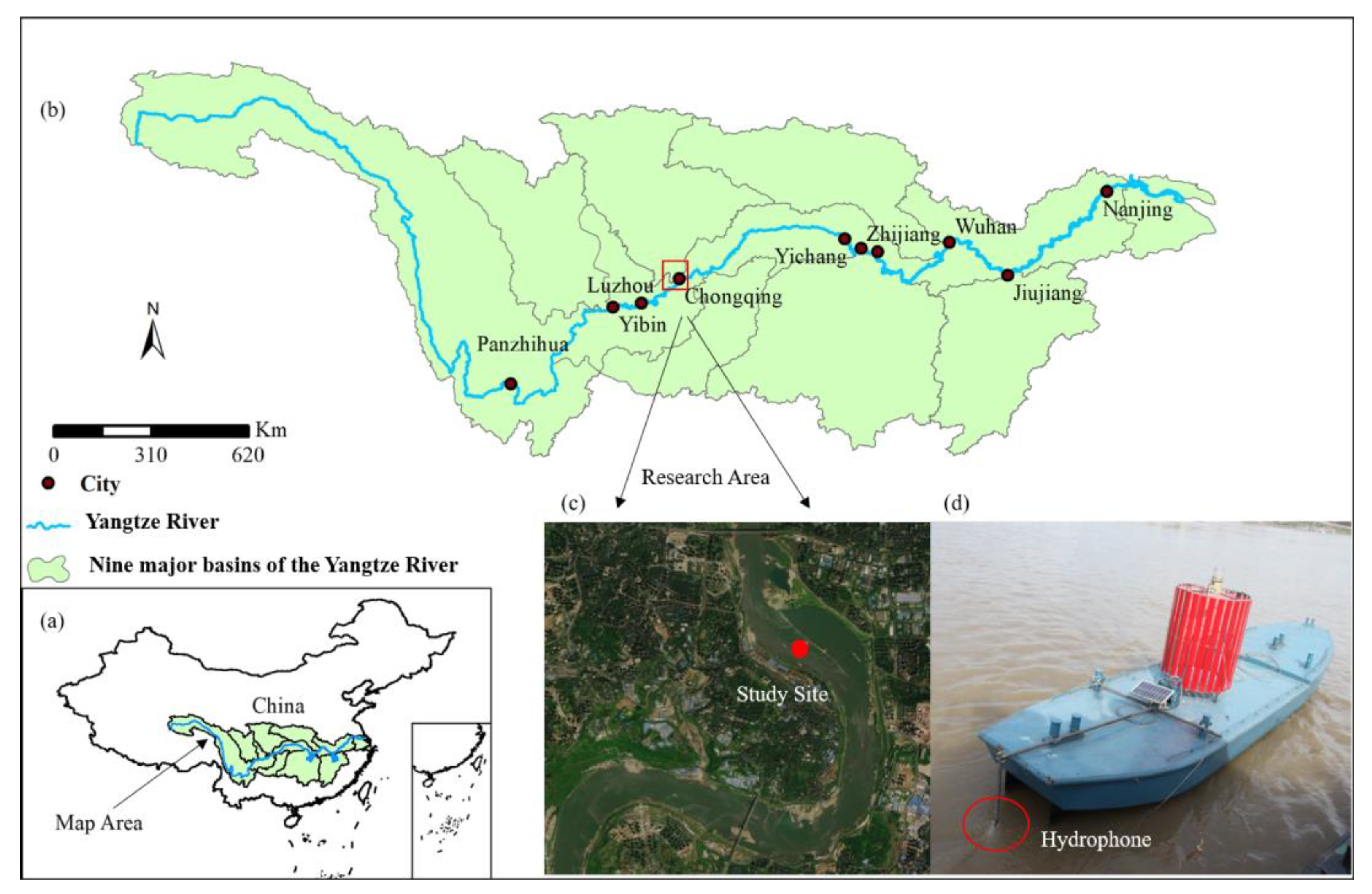
The Three Gorges Reservoir (TGR) backwater area is approximately 660 km long, stretching from Yichang to Chongqing, China, as shown in Figure 1b. The permanent backwater zone stretched from the dam to Fuling after the TGR pool level increased to 175 m in 2008, and the fluctuation backwater region extended to Jiangjin [29]. Since the TGR’s trial impoundment, some local sections of the fluctuation backwater area have experienced problems with gravels obstructing navigation, particularly on the triangular moraine in the upper reaches of the Yangtze River, as shown in Figure 1c. The channel’s minimum width is about 60 m, the water depth is about 3.0 m during low levels, and the bend radius of the main channel is only about 600 m during the dry season. It is extremely difficult to ship during the dry season, and it is prone to dangerous situations, such as stranding. It has been regarded as one of the most sinister waterways in Chongqing, with the characteristics of being bent, narrow, shallow, and dangerous. After the trial impoundment at the 175 m water level of the TGR, riverbed scour intensity decreased from 2012, while the main sediment discharge period was postponed to the pre-flood ebb and flow period [30].
The fluctuation backwater area returns to the natural channel in the dry season stage when the water level of the TGR drops from 175 m to 145 m (April to June). Meanwhile, with the rapid decrease in the water level along the reservoir, the increase in hydraulic power has generated a peak in bedload transport [29]. As a result, the sampling period was chosen every year, from April to June.
2.2. Acoustic Monitoring
The core of the acoustic instrumentation in this field observation is the Song Meter SM2M+ Marine Recorder (Wildlife Acoustics, Inc., Maynard, MA, USA), which features flexible scheduling, extremely low power consumption, and 16-bit digital recording in a cost-effective and easy-to-use package. The hydrophone is placed within a 79.4-cm-long, 16.5-cm-diameter PVC pipe, with the working depth reaching up to 150 m. It is equipped with two channels that can set output parameters (sampling frequency, gain, filter, etc.). The sensitivity of the hydrophone is calibrated to 1 dB resolution by the hydrophone manufacturer. The device allows sample rates from 4 kHz to 384 kHz. The recorded data can be stored on the SD card in WAV or WAC format, and the maximum storage capacity of the memory card is 128 G. The recorder is powered by 32 battery slots, and 32 alkaline batteries can be used for 600 h of recording time. The sampling frequency of 32 kHz is chosen based on the Nyquist sampling theorem and the results of Barton [23]. The operator can store cell batteries according to a specific case for long-term observation. The sound information recorded by the hydrophone is viewed in the Song Scope software, which is a data browser for the visual presentation of audio data. In addition, it provides a graph viewer with a powerful classification algorithm that can automatically scan the data for the target mode.
The experimental apparatus is mounted in a stainless-steel frame suspended from a boat. To avoid interference from flow resistance and floating objects, the frame is submerged 1 m underwater, as shown in Figure 1d.
2.3. Acoustic Signal Pretreatment
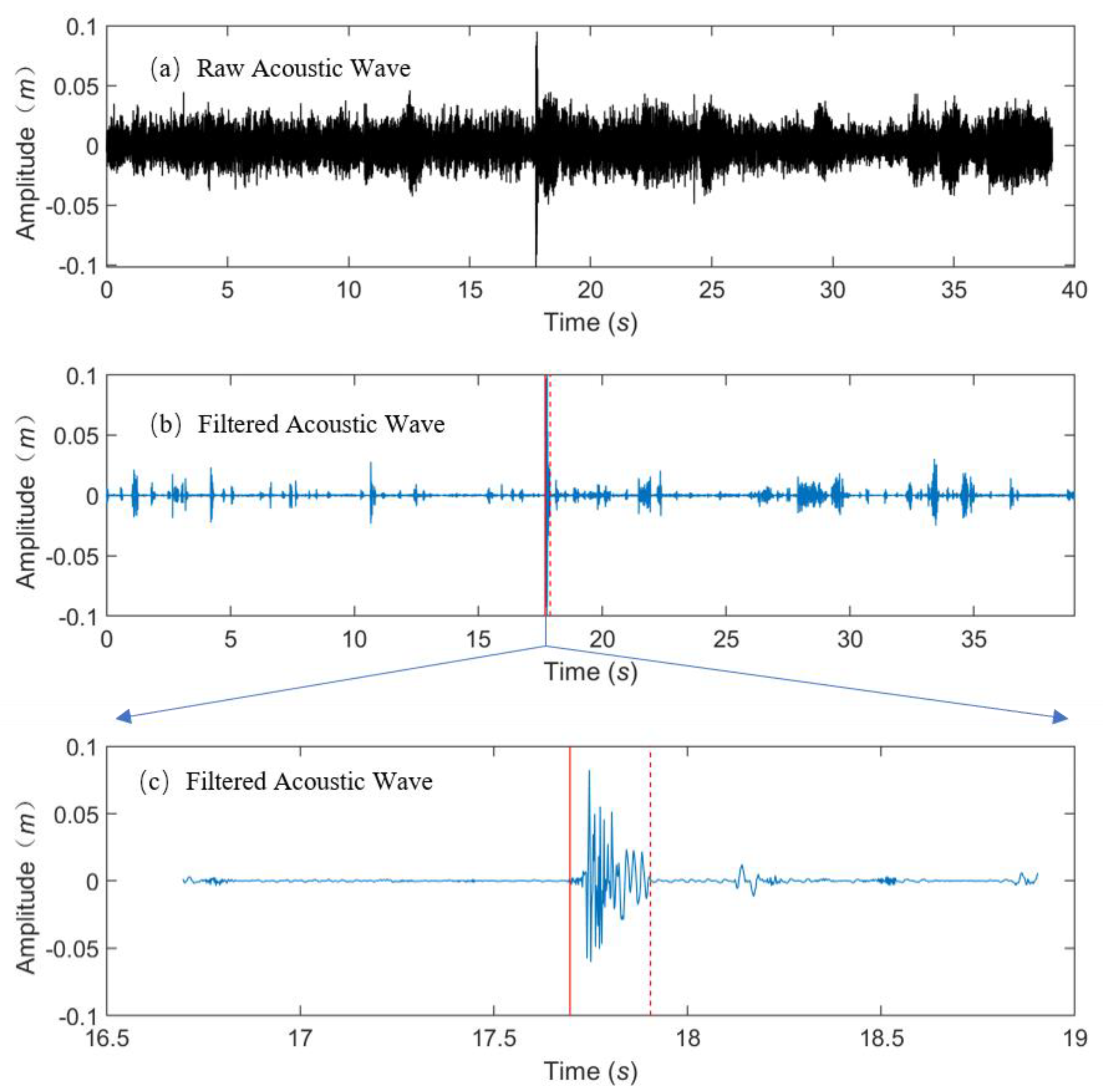
Hydrophones record the acoustic waves emitted by river environments, including sounds generated by moving bedload particles, ship engines, and flow turbulence, in which the sound of the moving bedload is the target signal that needs to be analyzed (see Figure 2a). If the target signal can be detected and extracted from the raw signal, it can greatly reduce the workload and improve the accuracy of the results. Preprocessing is the first key step in audio signal analysis. The preprocessing of the audio signal mainly includes the steps of framing, windowing, noise reduction, and endpoint detection [31,32]. The original audio signal has time-variation characteristics, but its characteristics are relatively stable in a short time range. Framing is the process of dividing the audio into several small segments with stable acoustic characteristics. Windowing can make the framed signal continuous. In this paper, the Hanning window was selected as the window function [33]. Signal noise reduction is essentially a process of target analysis and target signal extraction. Spectral subtraction is a sound signal enhancement method that uses the statistical stability of noise and is based on the fact that additional noise is irrelevant to the target sound [34,35]. The advantages of this method are that (i) it is easy to compute; (ii) it is easy to implement in real time; and (iii) the enhancement effect is obvious. In this paper, spectral subtraction is selected for noise reduction (see Figure 2b). The endpoint detection of an audio signal can distinguish between valid and invalid signal segments, extract the start point and end point of a valid signal segment in time [36,37], and can also be used to count the number of collisions between moving particles (see Figure 2c).
3. Results
3.1. Peak Frequency
The signal frequency characteristic is produced following the Fourier transform of the preprocessed acoustic signal. The distribution of the acoustic signal amplitude at each frequency can be seen in the frequency spectrum. The single collision acoustic signal is directly employed as a frame signal to calculate the two-dimensional frequency spectrum since its lifetime is very short (i.e., 5 ms–35 ms) and the frequency spectrum is constant within a very short time scale (i.e., 10 ms–30 ms). The peak frequency is recorded as , which is defined as the frequency that corresponds to the maximum power spectral density (PSD) [38]. Based on actual field observations, the main audio signals collected, in addition to the sound of moving bedload particles, are the sound of the ship engine and the flow turbulence. As a result, these three types of acoustic signals are chosen as analysis objects.
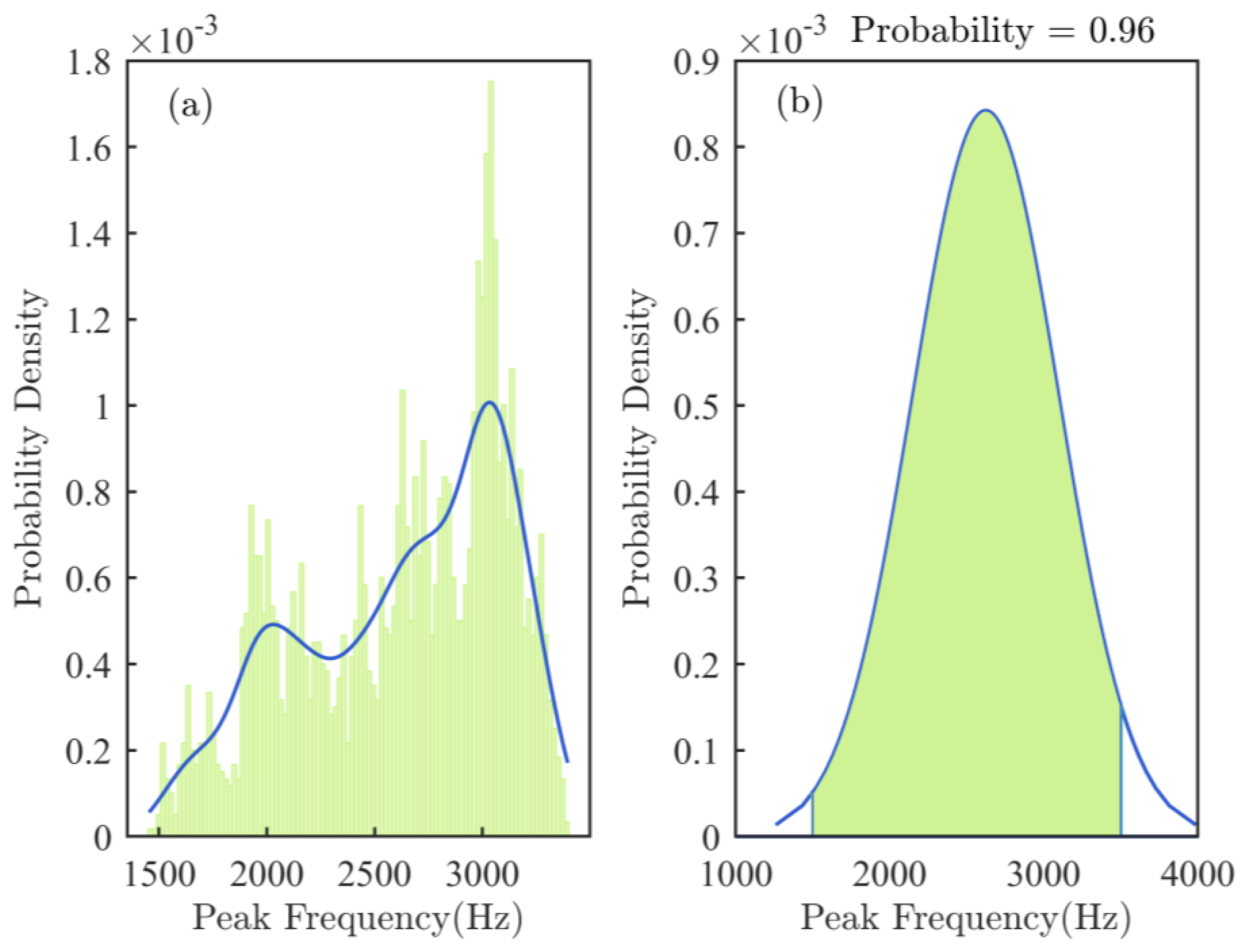
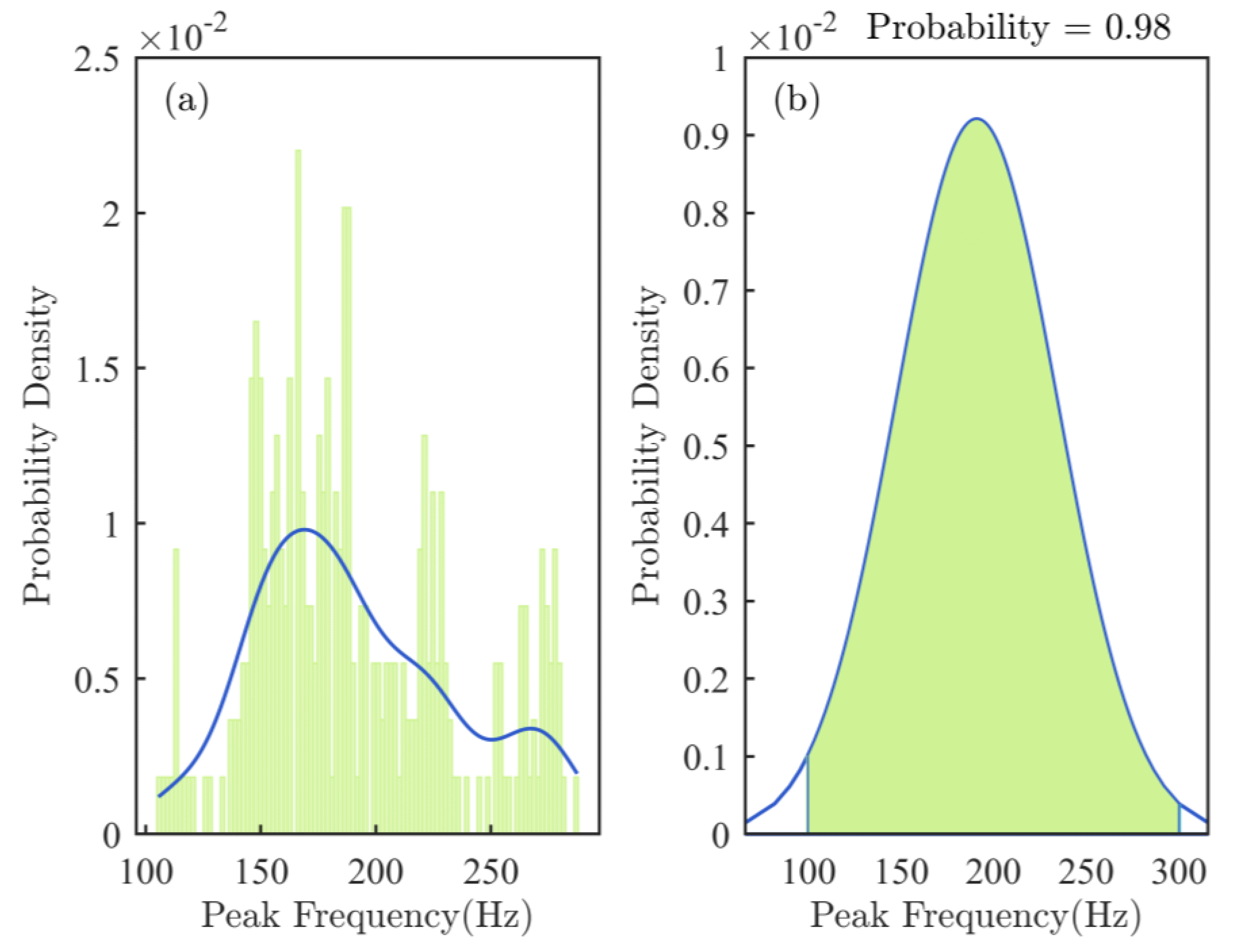
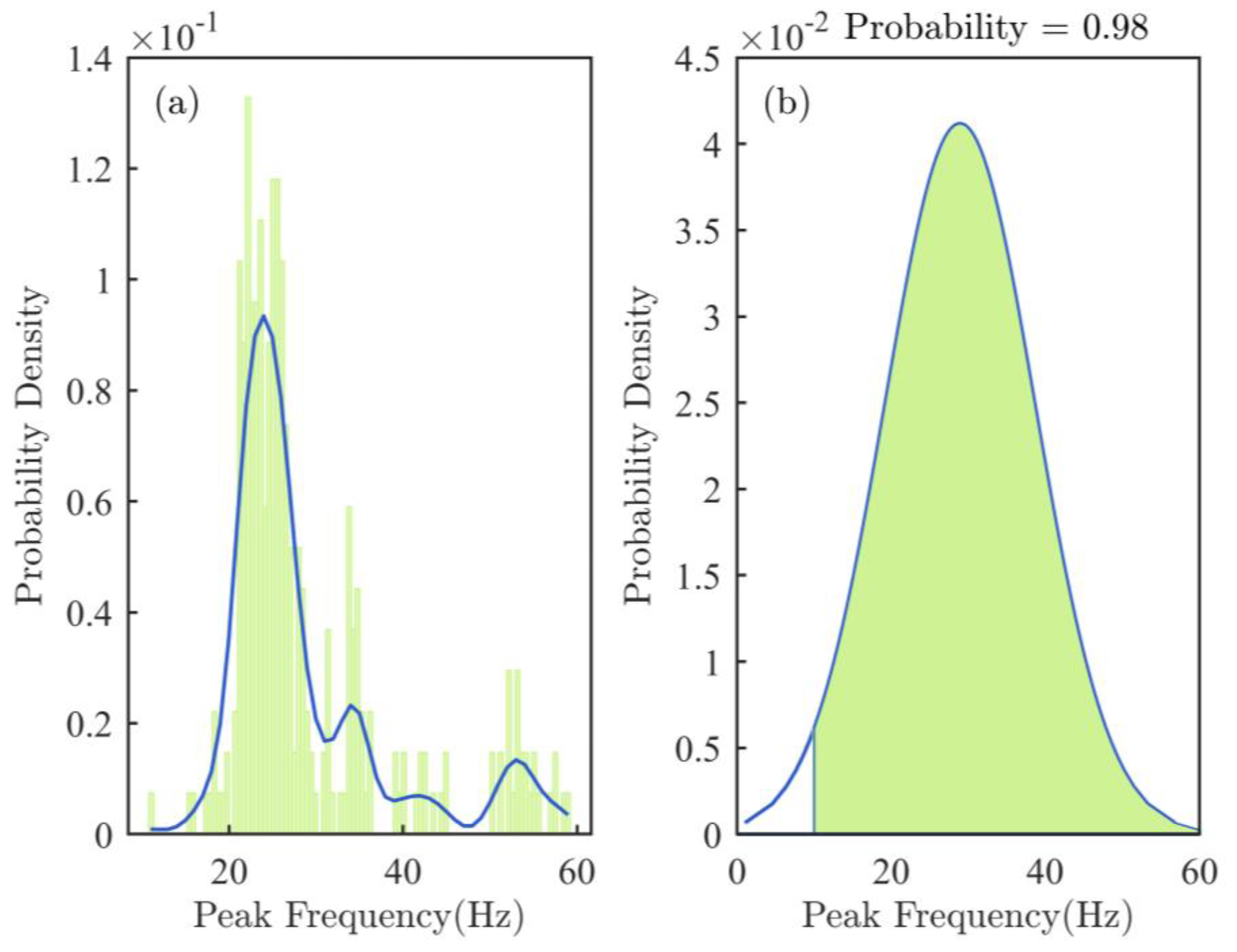
The hydrophone data from April to May 2015 and March to June 2016 are analyzed using autonomous programming in order to calculate the of the moving gravel particles, ship engines, and flow turbulence. Figure 3a shows a frequency histogram and probability distribution fitting curve for the moving gavel (denoted as ), and Figure 3b is an example of the probability, where the shaded area represents the probability value of falling within the range of 1500 and 3500 Hz with a value of 0.96. The probability distributions of ship engine () and flow turbulence (denoted as ) are shown in Figure 4 and Figure 5, respectively. Figure 4b displays a probability value of 0.98 for in the frequency range of 100–300 Hz, while Figure 5b displays a probability value of 0.97 for in the frequency range of 10–60 Hz.
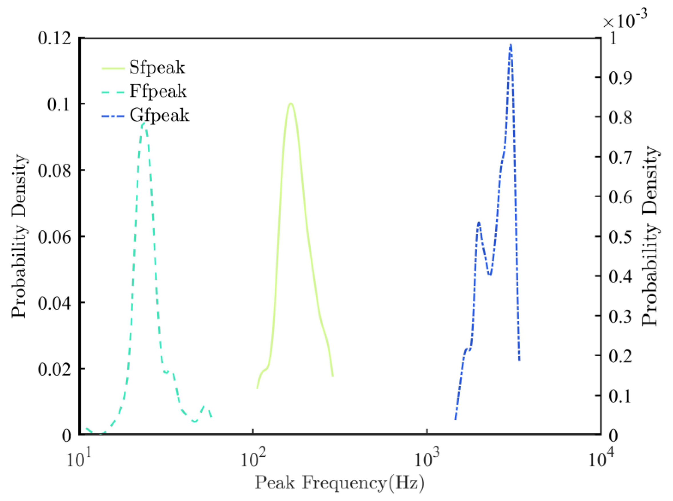
Figure 6 illustrates that the distribution differs significantly from that of the ship engine and flow turbulence. The frequency range of is 1500–3500 Hz and is influenced by particle size, shape, and material [39,40]. is primarily between 100 and 300 Hz and is influenced by the type of ship engine used. is primarily between 10 and 60 Hz and is simply influenced by flow conditions, exhibiting good stability. The can be utilized as a characteristic parameter to distinguish the sound of gravel movement in complicated audio signals during field observation due to the great differences between gravel particles, ship engines, and flow turbulence.
3.2. Pitch Frequency
The pitch period is the length of time it takes for the vocal folds to open and close during speech signals. The pitch period is the duration of the vocal folds’ vibration, and its inverse is known as the pitch frequency (). The characterizes an essential aspect of the speech excitation source and is a critical speech signal characteristic parameter. Pitch detection is the process of estimating the pitch period, and the ultimate goal is to identify the trajectory curve of the pitch period variation that most closely resembles the frequency of vocal fold vibration. Pitch detection is an essential component of many speech signal processing systems and is useful for a variety of applications, such as voice recognition, speech analysis and synthesis, articulatory organ disease diagnostics, language training for the hearing impaired, and many others [41,42]. Even though it differs from the audio signal produced by the vibration of a human vocal cord, the audio signal of a moving gravel collision has pitch characteristics. As a result, can be used to analyze the moving gravel audio signal as an acoustic feature parameter.
The auto correlation function (ACF), average amplitude difference function (AMDF), cepstrum method, wavelet transform method, and numerous other established methods are currently representative pitch detection methods. ACF has better performance and is more commonly used for noisy audio signals. The pitch period corresponds to the time delay at which the autocorrelation function exclusion point is at its greatest in the actual application, which typically calculates the autocorrelation function of the audio signal first. The entire computational process is implemented using autonomous programming. A statistical analysis of all the data is performed to determine the probability density distribution of the for the three different types of sound source signals—moving gravel particles, ship engines, and flow turbulence.
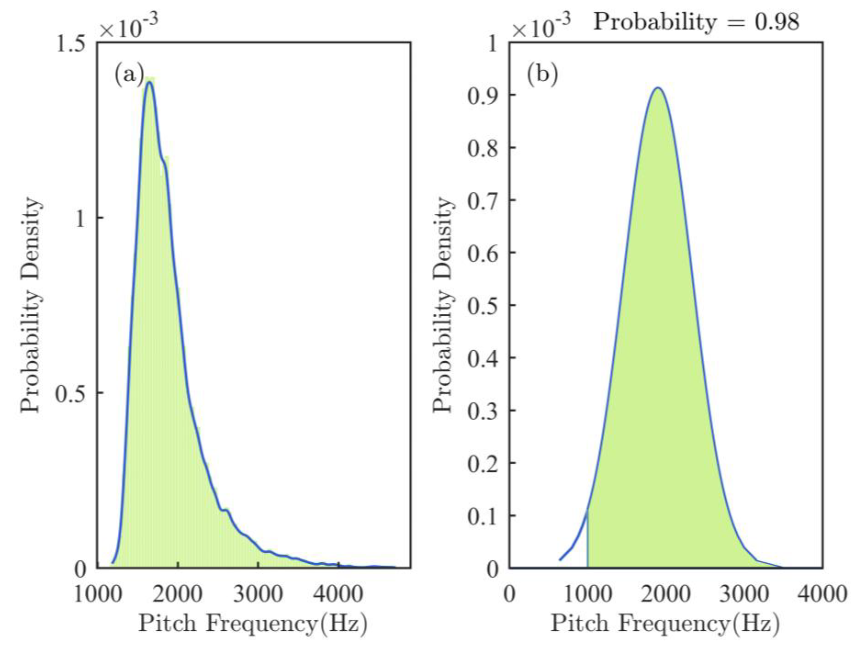
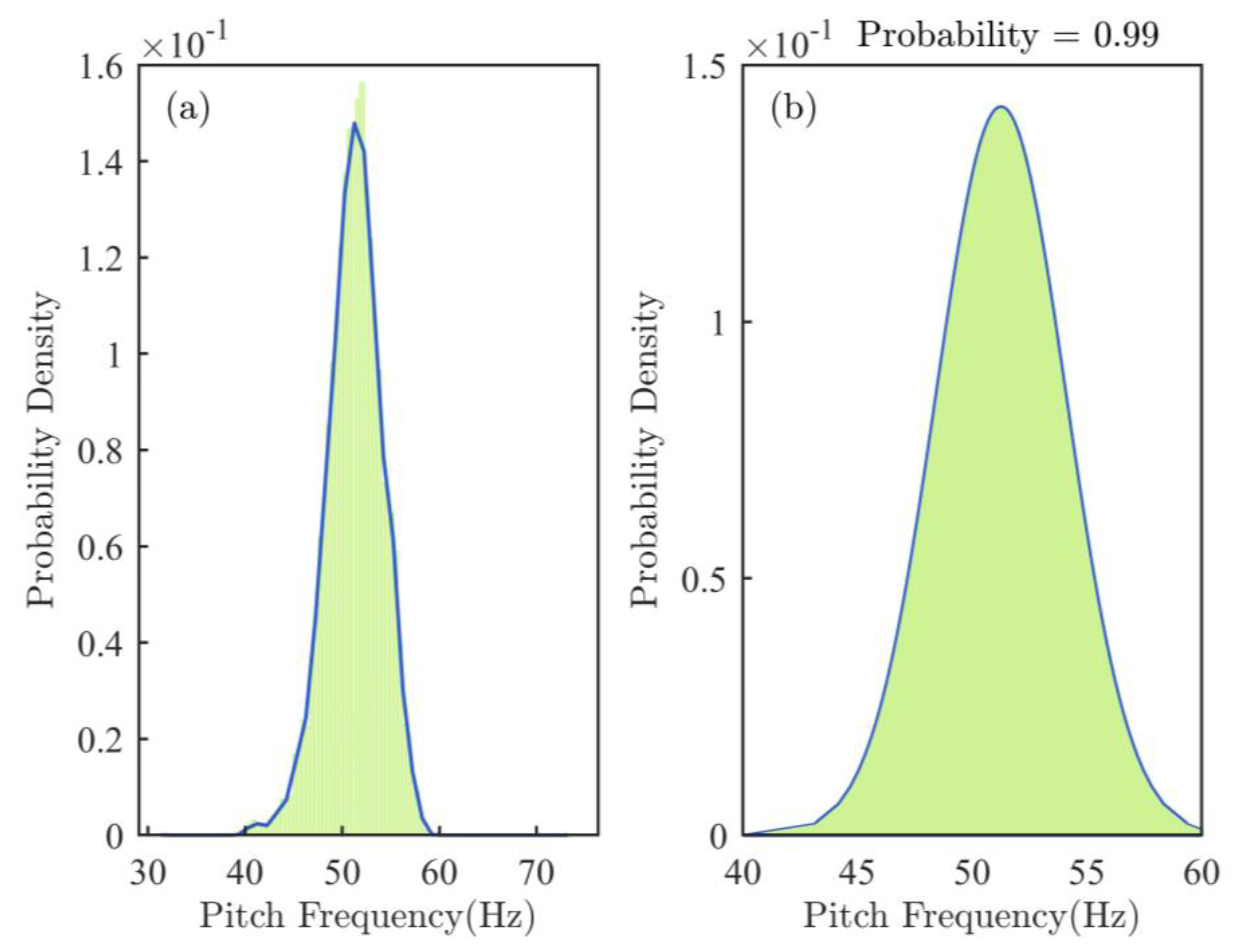
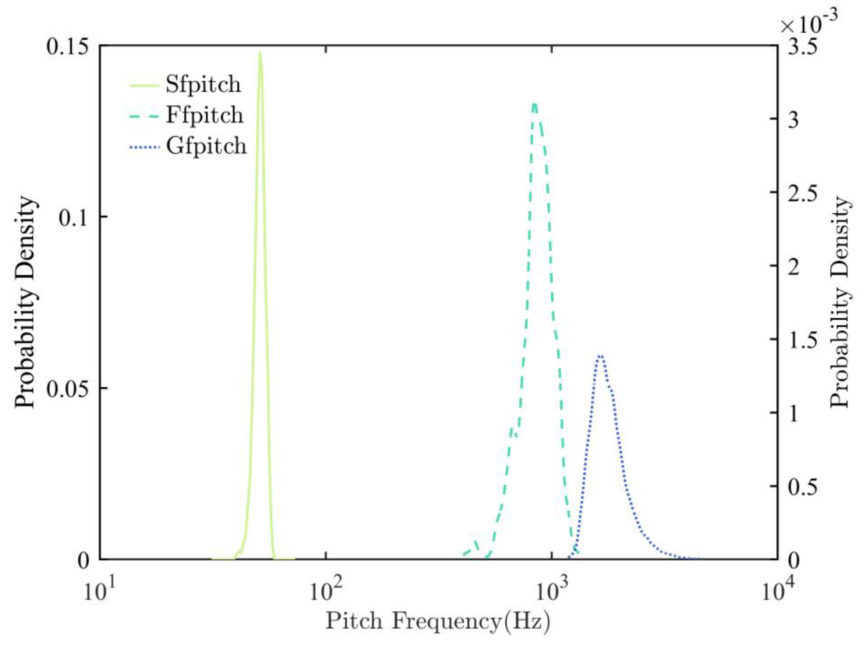
The probability density distribution of the moving gravel pitch frequency, denoted as , is shown in Figure 7. Figure 7a displays the frequency histogram and probability distribution fitting curve, while Figure 7b displays a sample probability plot produced by the capaplot function. The shaded area represents a probability of 0.97 that is between 1000 and 3500 Hz. Figure 8 and Figure 9 depict the probability distributions of the ship engine (denoted as ) and the flow turbulence (denoted as ), respectively. Figure 8b shows a probability value of 0.99 for at 400–1400 Hz, and Figure 9b shows a probability value of 0.99 for at 40–60 Hz. Figure 10 shows that the probability of the distribution of the pitch frequencies of gravel particles, ship engines, and flow turbulence varies significantly. Figure 10 shows that the gravel sediment signals have a that distinguishes them from the other two acoustic signals. As such, the can be used as a parameter to identify gravel particle sounds.
3.3. Energy Eigenvector
A wavelet transform can be used to pyramid decompose an audio signal, and a multi-level pyramid decomposition can be used to break the signal down into a collection of coefficients at different scales. Wavelet coefficients with larger values carry more signal energy, whereas those with smaller values carry less. What is important is the information about energy represented by these coefficients. Because of the large number of wavelet coefficients, it is impractical to use them directly as feature parameters. As a result, the total energy of the audio signal at each scale can be solved as an energy eigenvector for signal identification after wavelet transformation. If the audio signal is wavelet transformed in layers, the energy eigenvector is calculated by the following equation [43]:
where represents the set of the high-frequency coefficients of resolution level after wavelet decomposition, D represents the high-frequency, represents the low-frequency coefficients of the highest level after wavelet decomposition, A represents the low frequency, j and J represent the wavelet decomposition resolution level, k represents the kth wavelet coefficient at the jth resolution level, is the high-frequency wavelet energy at the jth level, d represents the high frequency as in D, is the highest-order low-frequency wavelet energy, and a represents the low-frequency.
E is the total energy of the high-frequency and low-frequency coefficients after the decomposition of J levels and is computed as follow [44]:
Finally, we define the normalized T, which represents the normalized energy eigenvector of the vector composed of and , for the resolution levels j = 1, 2,..., J.
The decomposition scale J is taken as 6, and the wavelet basis function is “db5” by comparing the computation outcomes of several groups. The energy eigenvectors of the audio signals of gravel particles, ship engines, and flow turbulence are generated by wavelet decomposition. Table 1, Table 2 and Table 3 list some typical results in which some values of parameters are displayed as 0 after rounding up/down the fifth digit number after the decimal point.
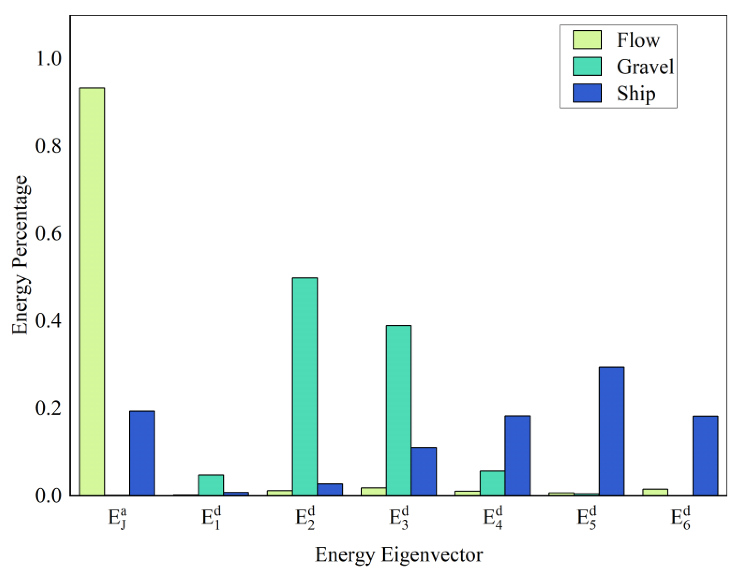
Table 1, Table 2 and Table 3 demonstrate that the energy eigenvector distributions of the three source signals differ significantly. It is seen from the tables that the gravel sound’s energy mostly spreads over the first-third order high frequency coefficients, accounting for more than 90% of the total energy. The ship engine’s energy concentrates on its low-frequency coefficients and its first four to six high-frequency coefficients. The low frequency coefficients, which distinguish the sound of the flow turbulence from the other two, have a significant concentration of energy (>90%). To compare the energy eigenvectors of gravel particles, ship engines, and flow turbulence sound signals, all samples collected are used to produce the average energy eigenvectors. The results of the calculated average energy eigenvectors for the grovel movement, ship engine, and flow turbulence are plotted in Figure 11. Figure 11 shows that the energy eigenvector differs depending on the distribution orders of the three signals. Such a difference makes it possible to use the energy eigenvector as a factor for detecting the sound of the bedload movement.
In conclusion, the distribution of , , and the energy eigenvector are determined by analyzing the sounds of gravel particles, ship engines, and flow turbulence. These feature characteristics must first undergo some quantitative processing in order to be made available for extracting the bedload movement signals from complicated acoustic sources. A confidence interval of 0.95 is chosen to obtain the range of 1500–3500 Hz and the range of 1000–3500 Hz. The total energy on the high-frequency coefficients of the 1st–3rd order, denoted as T, should satisfy the inequality 0.95 < T < 1. When an audio signal meets the requirements of these three characteristic parameters, namely is between 1500 and 3500 Hz, is between 1000 and 3500 Hz, and total energy with T of the energy eigenvector over the high frequency coefficients of order 1–3 satisfies 0.95 < T < 1, then an audio signal is thought to result from the collision of moving gravels.
4. Discussion
More than 90% of the of the gravels detected by the hydrophone in this field observation are concentrated in the range of 1500–3500 Hz, which coincides with the dominant frequency at 3300 Hz emitted by the gravel collisions monitored by Belleudy et al. [45] with a hydrophone in the Isère River. Though few studies have hypothesized that the sound produced by sediment particle impacts can be heard in the medium frequency range (300–2000 Hz) mixed with the flow turbulence noise caused by agitated water or turbulent eddies [46], most studies have found that the sound signal from gravel collisions occurs in the high-frequency region of the spectrum [27,38,47]. These studies show that the acoustic signal of gravel collisions is higher than 2000 Hz, while Tsubaki et al. [48] claimed that the signal frequency was between 3.5–10 kHz. Bassett et al. [49] used data from a hydrophone located in a tidal channel and found that is between 4 and 20 kHz for moving particles (4 to 170 mm), which is much larger than the frequency range found in this paper. By establishing the frequency vs. particle size relationship, it is possible to detect the bedload movement using the signal frequency. For uniform particle size, the Thorne-proposed and central frequency () versus particle size relationship is the most commonly used. Thorne found a nearly inverse relationship between these distinct frequencies and particle size D(m) [12,13,22]. For example, the of a particle with a diameter of 100 mm was determined to be around 1 kHz and approximately 10 kHz for a particle with a diameter of 10 mm [40].
As previously noted, the frequency content of the moving gravel acoustic signal is influenced by flow conditions, as well as the size of the gravel grains and propagation effects [50]. To distinguish the gravel movement signal from background noise, Geay et al. [46] proposed three frequency ranges: (1) 1000–60,000 Hz represented the bed load acoustic signal; (2) 100–1000 Hz represented the turbulence at low flow; and (3) bed load sound at high flow. The flow turbulence signal is influenced by the flow velocity of the channel, as well as by flow obstacles caused by various hydrogeomorphic characteristics [34]. The noise produced by surface waves decreases as the ratio of water depth to bed surface roughness increases, according to Tonolla et al. [51]. More than 90% of the frequency range of the sound signal produced by the flow turbulence is concentrated in the range of 10–60 Hz, according to the observation data from the upper sections of the Yangtze River. The observations made along three major European rivers, the Danube, Sava, and Tisa, are consistent with the findings of this study. The typical noise spectrum has a maximum level that fluctuates between 20 and 40 Hz [52]. Geay et al. [46], proposed similar findings, estimating that flow turbulence noise accounts for approximately 5–20% of all sound energy, varies with hydrological conditions, and disperses over a narrow frequency range (10–100 Hz).
The results of the field observations along several rivers revealed that each location’s flow turbulence and ship engines were distinct. Some studies showed that the flow turbulence sounds had a frequency ranging between 200 and 500 Hz [53,54], which included the frequency range below 300 Hz revealed by Wenz’s curves for self-induced flow turbulence noise [55]. Miyamoto et al. [56] presented research on flow turbulence noise in the Columbia River. They found that the noise spectrum peaks were less than 200 Hz. Because of the various monitoring situations, there is a wide range of frequencies; however, the majority do not exceed 1000 Hz [38,47,51,57].
Flow turbulence noise is the primary factor affecting the effectiveness of passive monitoring systems. Aside from flow turbulence, the ship engine is another main source of noise in monitoring data. More than 90% of is concentrated in the 100–300 Hz range, according to the monitoring data presented in this paper. This range corresponds to Wenz’s finding that the dominant frequencies for ship noise components are typically between 20 and 200 Hz [55]. Furthermore, the first two results are included in Marshall’s range of 25 to 500 Hz for the most common ship engine frequencies [58]. Ship noise is divided into two parts in terms of quality: that produced by propeller cavitation and that produced by internal machinery (engines, generators, pumps, etc.) [59,60]. As a result, the recorded frequency range of the ship engine is wide and even slightly overlaps with the frequency range of the flow turbulence. Several studies have linked the type of ship propulsion and horsepower to ship engines. The ship engine frequency is proportional to the size and speed of the ship [60,61,62,63]. In many places, the propellers and engines of commercial maritime vessels are the primary sources of low-frequency noise (20–200 Hz), and noise levels have been increasing [60,64]. In order to assess the ecologically relevant levels of the medium- and high-frequency ship engines, a broadband recording system was used to record different types of ships located by automatic identification systems in four Danish marine habitats. The findings showed that much of the noise from ship engine noise was over a wide frequency range, even in the ultrasonic range [65]. Low-frequency noise (below 1 kHz) was thought to be caused by spinning equipment and cavitation (bubble formation and bursting), whereas noise above 5 kHz was thought to be caused primarily by cavitation of the ship’s propellers or bubbles produced by jet engines [66]. Propeller spinning alone produces relatively few noise sources on a regular basis [67]. Ship engines with data below 1000 Hz account for the majority of monitoring results [68,69,70].
Traditionally is used by researchers to detect the gravel movement; however, using a single characteristic parameter to extract the gravel motion from sound signals is far from sufficient and is not accurate. In addition to the , the and the energy eigenvector are proposed in this study to improve the accuracy of the detection of gravel movement. Pitch detection has been a major research topic since the 1970s and is critical to many applications of speech signal processing. Several academics have proposed various pitch-detecting methods. Although progress is being made in the recognition of speech signals with noise, most studies have focused on the detection of clean audio signals [71,72,73]. Signal recognition is hampered by noise, which also reduces the accuracy of the pitch estimate [74,75,76]. Furthermore, as is employed as a feature parameter for the first time to detect gravel movement in this study, there are no previous studies for comparison. The results of this study demonstrates that could be employed as a feature parameter to detect the gravel movement.
The energy vector used in this paper is the time series of the original sound signal normalized by wavelet decomposition. The energy parameter is mainly used in signal analysis to establish a relationship with the bedload transport rate [24,77,78,79,80], and most of the vibration signal amplitude thresholds are used to identify whether the signal is a gravel collision signal. Such a threshold is set according to field observation [20,81,82,83,84,85]. However, this setting is not applicable to the extraction of pebble movement sounds in complex environmental noise. As such, this paper proposes to combine three characteristic parameters to improve the detection accuracy of gravel movement at the riverbed.
5. Conclusions
This field study demonstrates that hydrophones can be used to monitor bedload movement in large gravel rivers. The study shows that significant future work is required to develop a hydrophone array if the practical application is to be expanded to large mountain rivers, such as the upper Yangtze River. This is because field measurements are constrained by the placement of hydrophones. Nevertheless, the findings of this study show that acoustic methods can be used to monitor bedload movements in large gravel-bed rivers.
For the first time, three feature parameters, namely , , and energy eigenvector, are proposed in this paper to improve the accuracy of the detection of the gravel movement in large rivers. The , , and the energy eigenvector characteristics are determined through the processing of the field raw audio data. When the calculated is in the range of 1500–3500 Hz, the calculated is in the range of 1000–3500 Hz, and the total energy of the energy eigenvector on the 1st–3rd order high frequency coefficients is within 0.95–1 for the audio signal collected, it can almost be sure that the segment of the audio signal is produced by the gravel movement. Otherwise, the audio signal is just flow turbulence and ship engines. This finding would be significant for river management.
Author Contributions
Conceptualization, M.T. and S.Y.; methodology, M.T. and P.Z.; validation, M.T.; formal analysis, M.T. and P.Z.; re-sources, S.Y.; data curation, M.T.; writing—original draft preparation, M.T.; writ-ing—review and editing, M.T., S.Y. and P.Z.; project administration, S.Y.; funding acquisition, S.Y. All authors have read and agreed to the published version of the manuscript.
Funding
This research was funded by the Three Gorges Follow-up Scientific Research Project of China (Research and Application of the Prototype Observation Technology of Gravel Transport by the Pres-sure Method in the Fluctuating Backwater Area of the Three Gorges Reservoir, Project No.: 2017-31-1).
Data Availability Statement
The data presented in this study are available on request from the corresponding author.
Conflicts of Interest
The authors declare no conflict of interest.
References
- Rigby, J.R.; Wren, D.G.; Kuhnle, R.A. Passive Acoustic Monitoring of Bed Load for Fluvial Applications. J. Hydraul. Eng. 2016, 142, 02516003. [Google Scholar] [CrossRef]
- Wilcock, P.R. Entrainment, displacement and transport of tracer gravels. Earth Surf. Process. Landf. 1997, 22, 1125–1138. [Google Scholar] [CrossRef]
- Ancey, C.; Bohorquez, P.; Bardou, E. Sediment transport in mountain rivers. Ercoftac Bull. 2014, 100, 37–52. [Google Scholar]
- Carrillo, V.; Petrie, J.; Timbe, L.; Pacheco, E.; Astudillo, W.; Padilla, C.; Cisneros, F. Validation of an Experimental Procedure to Determine Bedload Transport Rates in Steep Channels with Coarse Sediment. Water 2021, 13, 672. [Google Scholar] [CrossRef]
- Kociuba, W. The Role of Bedload Transport in the Development of a Proglacial River Alluvial Fan (Case Study: Scott River, Southwest Svalbard). Hydrology 2021, 8, 173. [Google Scholar] [CrossRef]
- Tian, Z.; Liu, Y.; Zhang, X.; Zhang, Y.; Zhang, M. Formation Mechanisms and Characteristics of the Marine Nepheloid Layer: A Review. Water 2022, 14, 678. [Google Scholar] [CrossRef]
- Tian, Z.; Jia, Y.; Chen, J.; Liu, J.P.; Zhang, S.; Ji, C.; Liu, X.; Shan, H.; Shi, X.; Tian, J. Internal solitary waves induced deep-water nepheloid layers and seafloor geomorphic changes on the continental slope of the northern South China Sea. Phys. Fluids 2021, 33, 053312. [Google Scholar] [CrossRef]
- Habersack, H.; Kreisler, A.; Rindler, R.; Aigner, J.; Seitz, H.; Liedermann, M.; Laronne, J.B. Integrated automatic and continuous bedload monitoring in gravel bed rivers. Geomorphology 2017, 291, 80–93. [Google Scholar] [CrossRef]
- Ryan, S.E.; Bunte, K.; Potyondy, J.P. Breakout Session II, Bedload-Transport Measurement: Data Needs, Uncertainty, and New Technologies. In Proceedings of the Federal Interagency Sediment Monitoring Instrument and Analysis Workshop, Flagstaff, AZ, USA, 9–11 September 2005; p. 14. [Google Scholar]
- Rickenmann, D. Bed-Load Transport Measurements with Geophones and Other Passive Acoustic Methods. J. Hydraul. Eng. 2017, 143, 03117004. [Google Scholar] [CrossRef]
- Reid, I.; Layman, J.T.; Frostick, L.E. The Continuous Measurement Of Bedload Discharge. J. Hydraul. Res. 1980, 18, 243–249. [Google Scholar] [CrossRef]
- Nakaya, H. Bimodal analysis of sediment transport in mountain torrents using hydrophones and sediment traps. Int. J. Eros. Control. Eng. 2009, 2, 54–66. [Google Scholar] [CrossRef] [Green Version]
- Vázquez-Tarrío, D.; Menéndez-Duarte, R. Assessment of bedload equations using data obtained with tracers in two coarse-bed mountain streams (Narcea River basin, NW Spain). Geomorphology 2015, 238, 78–93. [Google Scholar] [CrossRef]
- Rickenmann, D.; McArdell, B.W. Continuous measurement of sediment transport in the Erlenbach stream using piezoelectric bedload impact sensors. Earth Surf. Process. Landf. 2007, 32, 1362–1378. [Google Scholar] [CrossRef]
- Barrière, J.; Krein, A.; Oth, A.; Schenkluhn, R. An advanced signal processing technique for deriving grain size information of bedload transport from impact plate vibration measurements. Earth Surf. Process. Landf. 2015, 40, 913–924. [Google Scholar] [CrossRef]
- Mao, L.; Carrillo, R.; Escauriaza, C.; Iroume, A. Flume and field-based calibration of surrogate sensors for monitoring bedload transport. Geomorphology 2016, 253, 10–21. [Google Scholar] [CrossRef] [Green Version]
- Tsutsumi, D.; Fujita, M.; Nonaka, M. Transport measurement with a horizontal and a vertical pipe microphone in a mountain stream: Taking account of particle saltation. Earth Surf. Process. Landf. 2018, 43, 1118–1132. [Google Scholar] [CrossRef]
- Uchida, T.; Sakurai, W.; Iuchi, T.; Izumiyama, H.; Borgatti, L.; Marcato, G.; Pasuto, A. Effects of episodic sediment supply on bedload transport rate in mountain rivers. Detecting debris flow activity using continuous monitoring. Geomorphology 2018, 306, 198–209. [Google Scholar] [CrossRef]
- Mizuyama, T. Measurement of bed load with the use of hydrophones in mountain torrents. IAHS Pulication 2003, 283, 222–227. [Google Scholar]
- Nicollier, T.; Rickenmann, D.; Hartlieb, A. Field and flume measurements with the impact plate: Effect of bedload grain-size distribution on signal response. Earth Surf. Process. Landf. 2021, 46, 1504–1520. [Google Scholar] [CrossRef]
- Gray, J.R.; Gartner, J.W.; Anderson, C.W.; Fisk, G.G.; Glysson, G.D.; Gooding, D.J.; Hornewer, N.J.; Larsen, M.C.; Macy, J.P.; Rasmussen, P.P.; et al. Surrogate Technologies for Monitoring Suspended-Sediment Transport in Rivers. In Sedimentology of Aqueous Systems; Poleto, C., Charlesworth, S., Eds.; Wiley-Blackwell: Oxford, UK, 2010; pp. 3–45. [Google Scholar]
- Mühlhofer, L. Untersuchungen über die Schwebstoff-und Geschiebeführung des Inn nächst Kirchbichl (Tirol). Die Wasserwirtsch. 1933, 1–6. [Google Scholar]
- Barton, J.S. Passive Acoustic Monitoring of Coarse Bedload in Mountain Streams. Ph.D. Thesis, The Pennsylvania State University, State College, PA, USA, 2006. [Google Scholar]
- Barton, J.S.; Slingerland, R.L.; Pittman, S.; Gabrielson, T.B. Monitoring Coarse Bedload Transport with Passive Acoustic Instrumentation: A Field Study. US Geol. Surv. Sci. Investig. Rep. 2010, 5091, 38–51. [Google Scholar]
- Krein, A.; Schenkluhn, R.; Kurtenbach, A.; Bierl, R.; Barrière, J. Listen to the sound of moving sediment in a small gravel-bed river. Int. J. Sediment Res. 2016, 31, 271–278. [Google Scholar] [CrossRef]
- Petrut, T.I.; Geay, T.; Gervaise, C.; Belleudy, P.; Zanker, S. Passive Acoustic Measurement of Bedload Grain Size Distribution using the Self-Generated Noise. Hydrol. Earth Syst. Sci. 2017, 22, 767–787. [Google Scholar] [CrossRef] [Green Version]
- Geay, T.; Zanker, S.; Misset, C.; Recking, A. Passive Acoustic Measurement of Bedload Transport: Toward a Global Calibration Curve? J. Geophys. Res. Earth Surf. 2020, 125, e2019JF005242. [Google Scholar] [CrossRef]
- Le Guern, J.; Rodrigues, S.; Geay, T.; Zanker, S.; Hauet, A.; Tassi, P.; Claude, N.; Jugé, P.; Duperray, A.; Vervynck, L. Relevance of acoustic methods to quantify bedload transport and bedform dynamics in a large sandy-gravel-bed river. Earth Surf. Dynam. 2021, 9, 423–444. [Google Scholar] [CrossRef]
- Xiao, Y.; Li, W.; Yang, S. Hydrodynamic-sediment transport response to waterway depth in the Three Gorges Reservoir, China. Arab. J. Geosci. 2021, 14, 775. [Google Scholar] [CrossRef]
- Lingling, Z.; Jun, L.; Jing, Y. Sediment Erosion and Deposition in the Tail Area of Three Gorges Reservoir. J. Yangtze River Sci. Res. Inst. 2018, 35, 142–146+156. [Google Scholar]
- Rabiner, L.R.; Schafer, R.W. Theory and Applications of Digital Speech Processing; Prentice Hall Press: Hoboken, NJ, USA, 2010; Volume 30, ISBN 978-0-13-603428-5. [Google Scholar]
- Ackroyd, M.H. Digital Processing of Speech Signals. Electron. Power UK 1979, 25, 290. [Google Scholar] [CrossRef]
- Huang, X.; Acero, A.; Hon, H.-W. Spoken Language Processing: A Guide to Theory, Algorithm and System Development; Prentice Hall PTR: Hoboken, NJ, USA, 2001. [Google Scholar]
- Boll, S. Suppression of acoustic noise in speech using spectral subtraction. IEEE Trans. Acoust. Speech Signal Process. 1979, 27, 113–120. [Google Scholar] [CrossRef] [Green Version]
- Zhang, C.; Dong, M. An improved speech endpoint detection based on adaptive sub-band selection spectral variance. In Proceedings of the 2016 35th Chinese Control Conference (CCC), Chengdu, China, 27–29 July 2016; pp. 5033–5037. [Google Scholar]
- Zhang, Y.; Wang, K.; Yan, B. Speech endpoint detection algorithm with low signal-to-noise based on improved conventional spectral entropy. In Proceedings of the 2016 12th World Congress on Intelligent Control and Automation (WCICA), Guilin, China, 12–15 June 2016; pp. 3307–3311. [Google Scholar]
- Zhang, T.; Shao, Y.; Wu, Y.; Geng, Y.; Fan, L. An overview of speech endpoint detection algorithms. Appl. Acoust. 2020, 160, 107133. [Google Scholar] [CrossRef]
- Geay, T.; Zanker, S.; Petrut, T.; Recking, A. Measuring bedload grain-size distributions with passive acoustic measurements. E3S Web Conf. 2018, 40, 04010. [Google Scholar] [CrossRef]
- Thorne, P.D.; Foden, D.J. Generation of underwater sound by colliding spheres. J. Acoust. Soc. Am. 1988, 84, 2144–2152. [Google Scholar] [CrossRef]
- Thorne, P.D. An overview of underwater sound generated by interparticle collisions and its application to the measurements of coarse sediment bedload transport. Earth Surf. Dyn. 2014, 12, 531–543. [Google Scholar] [CrossRef] [Green Version]
- Roy, S.K.; Molla, K.I.; Hirose, K.; Hasan, K. Harmonic modification and data adaptive filtering based approach to robust pitch estimation. Int. J. Speech Technol. 2011, 14, 339–349. [Google Scholar] [CrossRef]
- Ben Messaoud, M.A.; Bouzid, A. Pitch estimation of speech and music sound based on multi-scale product with auditory feature extraction. Int. J. Speech Technol. 2016, 19, 65–73. [Google Scholar] [CrossRef]
- Rosso, O.A.; Martin, M.T.; Figliola, A.; Keller, K.; Plastino, A. EEG analysis using wavelet-based information tools. J. Neurosci. Methods 2006, 153, 163–182. [Google Scholar] [CrossRef]
- Yen, G.G.; Lin, K.-C. Wavelet packet feature extraction for vibration monitoring. IEEE Trans. Ind. Electron. 2000, 47, 650–667. [Google Scholar] [CrossRef] [Green Version]
- Belleudy, P.; Valette, A.; Graff, B. Passive Hydrophone Monitoring of Bedload in River Beds: First Trials of Signal Spectral Analyses. River Flow 2010, 18, 67–84. [Google Scholar]
- Geay, T.; Belleudy, P.; Gervaise, C.; Habersack, H.; Aigner, J.; Kreisler, A.; Seitz, H.; Laronne, J.B. Passive acoustic monitoring of bed load discharge in a large gravel bed river. J. Geophys. Res. Earth Surf. 2017, 122, 528–545. [Google Scholar] [CrossRef]
- Tonolla, D.; Acuña, V.; Lorang, M.S.; Heutschi, K.; Tockner, K. A field-based investigation to examine underwater soundscapes of five common river habitats. Hydrol. Process. 2010, 24, 3146–3156. [Google Scholar] [CrossRef]
- Tsubaki, R.; Kawahara, Y.; Zhang, X.-H.; Tsuboshita, K. A new geophone device for understanding environmental impacts caused by gravel bedload during artificial floods. Water Resour. Res. 2017, 53, 1491–1508. [Google Scholar] [CrossRef]
- Bassett, C.; Thomson, J.; Polagye, B. Sediment-generated noise and bed stress in a tidal channel: SEDIMENT-GENERATED NOISE. J. Geophys. Res. Oceans 2013, 118, 2249–2265. [Google Scholar] [CrossRef]
- Medwin, H. Sounds in the Sea; Cambridge University Press: Cambridge, UK, 2005. [Google Scholar]
- Tonolla, D.; Lorang, M.S.; Heutschi, K.; Tockner, K. A flume experiment to examine underwater sound generation by flowing water. Aquat. Sci. 2009, 71, 449–462. [Google Scholar] [CrossRef] [Green Version]
- Vračar, M.S.; Mijić, M. Ambient noise in large rivers (L). J. Acoust. Soc. Am. 2011, 130, 1787–1791. [Google Scholar] [CrossRef] [PubMed]
- Bass, S.J.; Hay, A.E. Ambient noise in the natural surf zone: Wave-breaking frequencies. IEEE J. Oceanic Eng. 1997, 22, 411–424. [Google Scholar] [CrossRef]
- Lugli, M.; Yan, H.Y.; Fine, M.L. Acoustic communication in two freshwater gobies: The relationship between ambient noise, hearing thresholds and sound spectrum. J. Comp. Physiol. A 2003, 189, 309–320. [Google Scholar] [CrossRef]
- Wenz, G.M. Acoustic Ambient Noise in the Ocean: Spectra and Sources. J. Acoust. Soc. Am. 1962, 34, 1936–1956. [Google Scholar] [CrossRef]
- Miyamoto, R.T.; McConnell, S.O.; Anderson, J.J.; Feist, B.E. Underwater noise generated by Columbia River hydroelectric dams. J. Acoust. Soc. Am. 1989, 85, S127. [Google Scholar] [CrossRef]
- Mason, T.; Priestley, D.; Reeve, D.E. Monitoring near-shore shingle transport under waves using a passive acoustic technique. J. Acoust. Soc. Am. 2007, 122, 11. [Google Scholar] [CrossRef]
- Marshall, S.W. Depth dependence of ambient noise. IEEE J. Ocean. Eng. 2005, 30, 275–281. [Google Scholar] [CrossRef]
- Wales, S.C.; Heitmeyer, R.M. An ensemble source spectra model for merchant ship-radiated noise. J. Acoust. Soc. Am. 2002, 111, 1211–1231. [Google Scholar] [CrossRef] [PubMed]
- Hildebrand, J. Anthropogenic and natural sources of ambient noise in the ocean. Mar. Ecol. Prog. Ser. 2009, 395, 5–20. [Google Scholar] [CrossRef] [Green Version]
- Kipple, B.; Gabriele, C. Underwater Noise from Skiffs to Ships; Citeseer: Princeton, NJ, USA, 2004; pp. 172–175. [Google Scholar]
- Aguilar Soto, N.; Johnson, M.; Madsen, P.T.; Tyack, P.L.; Bocconcelli, A.; Fabrizio Borsani, J. Does intense ship noise disrupt foraging in deep-diving Cuvier’s beaked whales (Ziphius cavirostris)? Marine Mammal. Sci. 2006, 22, 690–699. [Google Scholar] [CrossRef]
- Jensen, F.H.; Bejder, L.; Wahlberg, M.; Soto, N.A.; Johnson, M.; Madsen, P.T. Vessel noise effects on delphinid communication. Mar. Ecol. Prog. Ser. 2009, 395, 161–175. [Google Scholar] [CrossRef]
- Rolland, R.M.; Parks, S.E.; Hunt, K.E.; Castellote, M.; Corkeron, P.J.; Nowacek, D.P.; Wasser, S.K.; Kraus, S.D. Evidence that ship noise increases stress in right whales. Proc. R. Soc. B. 2012, 279, 2363–2368. [Google Scholar] [CrossRef] [Green Version]
- Hermannsen, L.; Beedholm, K.; Tougaard, J.; Madsen, P.T. High frequency components of ship noise in shallow water with a discussion of implications for harbor porpoises (Phocoena phocoena). J. Acoust. Soc. Am. 2014, 136, 1640–1653. [Google Scholar] [CrossRef] [Green Version]
- Hildebrand, J.A.; Mcdonald, M.A.; Calambokidis, J.; Balcomb, K. Whale Watch Vessel Ambient Noise in the Haro Strait; Report on cooperative agreement NA17RJ1231; Joint Institute for Marine Observations: Silver Spring, MD, USA, 2006. [Google Scholar]
- Scholik, A.R.; Yan, H.Y. Effects of Boat Engine Noise on the Auditory Sensitivity of the Fathead Minnow, Pimephales promelas. Environ. Biol. Fishes 2002, 63, 203–209. [Google Scholar] [CrossRef]
- Urick, R.J. Principles of Underwater Sound; McGraw-Hill Book Company: New York, NY, USA, 1983. [Google Scholar]
- Scrimger, P.; Heitmeyer, R.M. Acoustic source-level measurements for a variety of merchant ships. J. Acoust. Soc. Am. 1991, 89, 691–699. [Google Scholar] [CrossRef]
- McKenna, M.F.; Wiggins, S.M.; Hildebrand, J.A. Relationship between container ship underwater noise levels and ship design, operational and oceanographic conditions. Sci. Rep. 2013, 3, 1760. [Google Scholar] [CrossRef] [Green Version]
- Shahnaz, C.; Zhu, W.-P.; Ahmad, M.O. A Robust Pitch Estimation Algorithm in Noise. In Proceedings of the 2007 IEEE International Conference on Acoustics, Speech and Signal Processing-ICASSP’07, Honolulu, HI, USA, 16–20 April 2007; IEEE: Piscataway, NJ, USA, 2007; pp. IV-1073–IV-1076. [Google Scholar]
- Shahnaz, C.; Zhu, W.-P.; Ahmad, M.O. A pitch extraction algorithm in noise based on temporal and spectral representations. In Proceedings of the 2008 IEEE International Conference on Acoustics, Speech and Signal Processing, Las Vegas, NV, USA, 31 March–4 April 2008; IEEE: Piscataway, NJ, USA, 2008; pp. 4477–4480. [Google Scholar]
- Verteletskaya, E.; Sakhnov, K.; Simak, B. Pitch Detection Algorithms and Voiced/Unvoiced Classification for Noisy Speech. In Proceedings of the 2009 16th International Conference on Systems, Signals and Image Processing, Chalkida, Greece, 18–20 June 2009; IEEE: Piscataway, NJ, USA, 2009; pp. 1–5. [Google Scholar]
- Molla, M.K.; Hirose, K.; Minematsu, N.; Hasan, M.K. Pitch estimation of noisy speech signals using empirical mode decomposition. In Proceedings of the Eighth Annual Conference of the International Speech Communication Association, Antwerp, Belgium, 27–31 August 2007; p. 1648. [Google Scholar]
- Zhong, T.; Wang, W.; Lu, S.; Dong, X.; Yang, B. RMCHN: A Residual Modular Cascaded Heterogeneous Network for Noise Suppression in DAS-VSP Records. IEEE Geosci. Remote Sens. Lett. 2022, 20, 1–5. [Google Scholar] [CrossRef]
- Fu, Q.; Si, L.; Liu, J.; Shi, H.; Li, Y. Design and experimental study of a polarization imaging optical system for oil spills on sea surfaces. Appl. Opt. 2022, 61, 6330–6338. [Google Scholar] [CrossRef]
- Bogen, J. Bed load measurements with a new passive. Erosion and sediment transport measurement in rivers: Technological and methodological advances. Acoust. Sens. 2003, 12, 181. [Google Scholar]
- Rickenmann, D.; Turowski, J.M.; Fritschi, B.; Wyss, C.; Laronne, J.; Barzilai, R.; Reid, I.; Kreisler, A.; Aigner, J.; Seitz, H.; et al. Bedload transport measurements with impact plate geophones: Comparison of sensor calibration in different gravel-bed streams: IMPACT PLATE GEOPHONE CALIBRATION. Earth Surf. Process. Landf. 2014, 39, 928–942. [Google Scholar] [CrossRef]
- Fu, Q.; Luo, K.; Song, Y.; Zhang, M.; Zhang, S.; Zhan, J.; Li, Y. Study of Sea Fog Environment Polarization Transmission Characteristics. Appl. Sci. 2022, 12, 8892. [Google Scholar] [CrossRef]
- Yuan, L.; Yang, D.; Wu, X.; He, W.; Kong, Y.; Ramsey, T.S.; Degefu, D.M. Development of multidimensional water poverty in the Yangtze River Economic Belt, China. J. Environ. Manag. 2023, 325, 116608. [Google Scholar] [CrossRef]
- Zhao, C.; Cheung, C.F.; Xu, P. High-efficiency sub-microscale uncertainty measurement method using pattern recognition. ISA Trans. 2020, 101, 503–514. [Google Scholar] [CrossRef]
- Liu, F.; Zhao, X.; Zhu, Z.; Zhai, Z.; Liu, Y. Dual-microphone active noise cancellation paved with Doppler assimilation for TADS. Mech. Syst. Signal Process. 2023, 184, 109727. [Google Scholar] [CrossRef]
- Turowski, J.M.; Rickenmann, D. Tools and cover effects in bedload transport observations in the Pitzbach, Austria. Earth Surf. Process. Landf. 2009, 34, 26–37. [Google Scholar] [CrossRef]
- Turowski, J.M.; Böckli, M.; Rickenmann, D.; Beer, A.R. Field measurements of the energy delivered to the channel bed by moving bed load and links to bedrock erosion. J. Geophys. Res. Earth Surf. 2013, 118, 2438–2450. [Google Scholar] [CrossRef] [Green Version]
- Turowski, J.M.; Wyss, C.R.; Beer, A.R. Grain size effects on energy delivery to the streambed and links to bedrock erosion. Geophys. Res. Lett. 2015, 42, 1775–1780. [Google Scholar] [CrossRef] [Green Version]
Figure 1.
(a) Map of the study region in the Yangtze River in China; (b) Zoom on the details of the Yangtze River; (c) Photo of study reach and sketch of the sampling site (red dot); (d) Photo of installation of a hydrophone in the river (red circle).
Figure 1.
(a) Map of the study region in the Yangtze River in China; (b) Zoom on the details of the Yangtze River; (c) Photo of study reach and sketch of the sampling site (red dot); (d) Photo of installation of a hydrophone in the river (red circle).

Figure 2.
An example of acoustic signal processing: (a) A recorded raw acoustic wave profile; (b) An acoustic wave after applying spectral subtraction noise reduction; (c) A close−up of the acoustic wave after applying noise reduction and endpoint detection.
Figure 2.
An example of acoustic signal processing: (a) A recorded raw acoustic wave profile; (b) An acoustic wave after applying spectral subtraction noise reduction; (c) A close−up of the acoustic wave after applying noise reduction and endpoint detection.

Figure 3.
Probability density distribution of the gravel peak frequency : (a) The vertical axis values of the histogram (green part) indicate the probability of the sample falling in each frequency interval, and the blue curve is the probability distribution fitting curve; (b) the probability value (shaded green area) calculated using autonomous programming.

Figure 4.
Probability density distribution of the ship engine peak frequency : (a) The vertical axis values of the histogram (green part) indicate the probability of the sample falling in each frequency interval, and the blue curve is the probability distribution fitting curve; (b) the probability value (shaded green area) calculated using autonomous programming.

Figure 5.
Probability density distribution of the flow turbulence peak frequency : (a) The vertical axis values of the histogram (green part) indicate the probability of the sample falling in each frequency interval, and the blue curve is the probability distribution fitting curve; (b) the probability value (shaded green area) calculated using autonomous programming.

Figure 6.
Probability density distribution curves of the peak frequency for three types of acoustic signals. Preliminary calculations were attained by randomly extracting audio signal fragments from the original audio signal to be used as analysis samples. The curves in the image were generated by smoothing the results of the preliminary calculations to concentrate the distribution.

Figure 7.
Probability density distribution of the gravel pitch frequency : (a) The vertical axis values of the histogram (green part) indicate the probability of the sample falling in each frequency interval, and the blue curve is the probability distribution fitting curve; (b) the probability value (shaded green area) calculated using autonomous programming.

Figure 8.
Probability density distribution of the ship engine pitch frequency : (a) The vertical axis values of the histogram (green part) indicate the probability of the sample falling in each frequency interval, and the blue curve is the probability distribution fitting curve; (b) the probability value (shaded green area) calculated using autonomous programming.

Figure 9.
Probability density distribution of the flow turbulence pitch frequency : (a) The vertical axis values of the histogram (green part) indicate the probability of the sample falling in each frequency interval, and the blue curve is the probability distribution fitting curve; (b) the probability value (shaded green area) calculated using autonomous programming.

Figure 10.
Probability density distribution curve of pitch frequency for three types of acoustic signals. (The preliminary calculations are obtained by randomly extracting the audio signal fragments from the original audio signal to use as analysis samples. The curves in the image are plotted by smoothing the results of the preliminary calculations to concentrate the distribution.)

Figure 11.
Energy eigenvector distribution characteristics of three kinds of acoustic signals.


Table 1.
Energy eigenvector of moving gravel particle acoustic signal.
| Sample | S1 | S2 | S3 | S4 | S5 | S6 | S7 | S8 | S9 | S10 |
|---|---|---|---|---|---|---|---|---|---|---|
| 0.0011 | 0.0002 | 0.0002 | 0.0006 | 0.0001 | 0.0002 | 0.0000 | 0.0000 | 0.0001 | 0.0000 | |
| 0.0481 | 0.0635 | 0.0439 | 0.1048 | 0.0228 | 0.0517 | 0.2493 | 0.0915 | 0.0840 | 0.0773 | |
| 0.4988 | 0.5776 | 0.5018 | 0.5846 | 0.3253 | 0.7196 | 0.6354 | 0.5356 | 0.6362 | 0.7652 | |
| 0.3897 | 0.3100 | 0.4165 | 0.2534 | 0.6163 | 0.1941 | 0.1133 | 0.3262 | 0.2410 | 0.1403 | |
| 0.0569 | 0.0451 | 0.0358 | 0.0522 | 0.0345 | 0.0326 | 0.0020 | 0.0459 | 0.0356 | 0.0165 | |
| 0.0046 | 0.0019 | 0.0017 | 0.0035 | 0.0008 | 0.0012 | 0.0001 | 0.0007 | 0.0024 | 0.0006 | |
| 0.0009 | 0.0017 | 0.0002 | 0.0010 | 0.0003 | 0.0006 | 0.0000 | 0.0001 | 0.0007 | 0.0000 |
Table 2.
Energy eigenvector of ship engine acoustic signal.
| Sample | S1 | S2 | S3 | S4 | S5 | S6 | S7 | S8 | S9 | S10 |
|---|---|---|---|---|---|---|---|---|---|---|
| 0.5641 | 0.2158 | 0.4248 | 0.4410 | 0.3811 | 0.5584 | 0.2951 | 0.3432 | 0.4438 | 0.4935 | |
| 0.0089 | 0.0035 | 0.0026 | 0.0033 | 0.0027 | 0.0032 | 0.0019 | 0.0009 | 0.0016 | 0.0017 | |
| 0.0281 | 0.0327 | 0.0304 | 0.0219 | 0.0260 | 0.0249 | 0.0149 | 0.0121 | 0.0122 | 0.0238 | |
| 0.0490 | 0.0672 | 0.0644 | 0.0493 | 0.0892 | 0.0701 | 0.0397 | 0.0521 | 0.0360 | 0.0654 | |
| 0.1059 | 0.1787 | 0.0924 | 0.0713 | 0.1707 | 0.1078 | 0.0621 | 0.0854 | 0.0541 | 0.0980 | |
| 0.1347 | 0.0496 | 0.1479 | 0.0858 | 0.1229 | 0.0936 | 0.1306 | 0.1514 | 0.1106 | 0.1549 | |
| 0.1091 | 0.4525 | 0.2375 | 0.3274 | 0.2073 | 0.1421 | 0.4557 | 0.3549 | 0.3417 | 0.1627 |
Table 3.
Energy eigenvector of flow turbulence acoustic signal.
| Sample | S1 | S2 | S3 | S4 | S5 | S6 | S7 | S8 | S9 | S10 |
|---|---|---|---|---|---|---|---|---|---|---|
| 0.9432 | 0.9490 | 0.9217 | 0.9337 | 0.9551 | 0.9394 | 0.9352 | 0.9608 | 0.9389 | 0.9501 | |
| 0.0002 | 0.0002 | 0.0002 | 0.0004 | 0.0002 | 0.0004 | 0.0005 | 0.0006 | 0.0001 | 0.0003 | |
| 0.0028 | 0.0028 | 0.0017 | 0.0025 | 0.0016 | 0.0038 | 0.0038 | 0.0041 | 0.0017 | 0.0023 | |
| 0.0121 | 0.0111 | 0.0144 | 0.0131 | 0.0055 | 0.0123 | 0.0123 | 0.0067 | 0.0113 | 0.0100 | |
| 0.0093 | 0.0080 | 0.0218 | 0.0132 | 0.0087 | 0.0117 | 0.0154 | 0.0065 | 0.0140 | 0.0100 | |
| 0.0199 | 0.0151 | 0.0250 | 0.0208 | 0.0147 | 0.0167 | 0.0184 | 0.0096 | 0.0173 | 0.0114 | |
| 0.0125 | 0.0138 | 0.0153 | 0.0163 | 0.0143 | 0.0157 | 0.0143 | 0.0116 | 0.0167 | 0.0159 |
Disclaimer/Publisher’s Note: The statements, opinions and data contained in all publications are solely those of the individual author(s) and contributor(s) and not of MDPI and/or the editor(s). MDPI and/or the editor(s) disclaim responsibility for any injury to people or property resulting from any ideas, methods, instructions or products referred to in the content. |
© 2023 by the authors. Licensee MDPI, Basel, Switzerland. This article is an open access article distributed under the terms and conditions of the Creative Commons Attribution (CC BY) license (https://creativecommons.org/licenses/by/4.0/).
Share and Cite
MDPI and ACS Style
Tian, M.; Yang, S.; Zhang, P. Detection of the Bedload Movement with an Acoustic Sensor in the Yangtze River, China. Water 2023, 15, 939. https://doi.org/10.3390/w15050939
AMA Style
Tian M, Yang S, Zhang P. Detection of the Bedload Movement with an Acoustic Sensor in the Yangtze River, China. Water. 2023; 15(5):939. https://doi.org/10.3390/w15050939
Chicago/Turabian StyleTian, Mi, Shengfa Yang, and Peng Zhang. 2023. "Detection of the Bedload Movement with an Acoustic Sensor in the Yangtze River, China" Water 15, no. 5: 939. https://doi.org/10.3390/w15050939
Note that from the first issue of 2016, this journal uses article numbers instead of page numbers. See further details here.