
Streamflow Estimation in a Mediterranean Watershed Using Neural Network Models: A Detailed Description of the Implementation and Optimization

Centro de Ciência e Tecnologia do Ambiente e do Mar (MARETEC-LARSyS), Instituto Superior Técnico, Universidade de Lisboa, Av. Rovisco Pais, 1, 1049-001 Lisboa, Portugal
*
Author to whom correspondence should be addressed.
Water 2023, 15(5), 947; https://doi.org/10.3390/w15050947
Submission received: 8 February 2023
/
Revised: 21 February 2023
/
Accepted: 24 February 2023
/
Published: 1 March 2023
(This article belongs to the Section Hydrology)
Abstract
:This study compares the performance of three different neural network models to estimate daily streamflow in a watershed under a natural flow regime. Based on existing and public tools, different types of NN models were developed, namely, multi-layer perceptron, long short-term memory, and convolutional neural network. Precipitation was either considered an input variable on its own or combined with air temperature as another input variable. Different periods of accumulation, average, and/or delay were considered. The models’ structures were optimized and automatically showed that CNN performed best, reaching, for example, a Nash–Sutcliffe efficiency of 0.86 and a root mean square error of 4.2 m3 s−1. This solution considers a 1D convolutional layer and a dense layer as the input and output layers, respectively. Between those layers, two 1D convolutional layers are considered. As input variables, the best performance was reached when the accumulated precipitation values were 1 to 5, and 10 days and delayed by 1 to 7 days.
1. Introduction
Accurate knowledge of streamflow is essential in a wide range of applications and studies, including the development of flood warning systems, hydroelectric reservoir operation, hydraulic structure design, fish production and survival, nutrient transport and water quality assessment, evaluation of long-term climate or land use change impacts, and the definition of water management policies [1,2]. Humphrey et al. [3] also state that an accurate and reliable streamflow forecast is crucial for the proper management and allocation of water resources, especially in areas with highly variable climate conditions and where there is not enough available data to adequately support decision-making.
According to Besaw et al. [4], streamflow estimation in gauged and/or ungauged areas can be performed based on conceptual, metric, physics-based, and data-driven methods. Conceptual methods only consider simplified conceptualizations of hydrological processes [5]. Methods classified as metric are based on the unit hydrograph theory, without considering hydrological features or processes [6]. Physically based models, also known as process-based models, rely on physical principles and, consequently, are suitable to provide insights into physical processes. However, these models often incorporate many simplifying assumptions and have requirements for large sets of data, with their calibration and validation processes being particularly laborious [7,8]. Finally, data-driven methods are empirical, are developed based on historical observations, and do not require information on physical processes [9]. Multiple linear regression (MLR) variations of autoregressive moving average (ARMA) or artificial neural networks (ANN) are examples of data-driven models.
Artificial neural networks are special types of machine-learning methods, which have been extensively used in streamflow estimation with promising results in the last decades because of the nonlinear nature of the rainfall–runoff relationship and the availability of long historical records [10]. In the review written by Maier et al. [11] of 210 published papers using ANN in the field of hydrology between 1999 and 2007, 90% were related to studies where the main goal was flow prediction (the other 10% were related to water quality variables). In the last few years, hydrologists have continued to investigate the ability of neural networks (NN) to predict river flow. For instance, Pham et al. [12] used a multilayer perceptron (MLP) neural network combined with the intelligent water drop algorithm, an advanced optimization algorithm for searching the global optima, to predict the streamflow in two stations on Vu Gia Thu Bon watershed, Vietnam. Hussain and Khan [13] tested a MLP, a support vector regression model, and a random forest model in forecasting the monthly streamflow in the Hunza river watershed, Pakistan. Sahoo et al. [14], Le et al. [15], Hauswirth et al. [16], and Althoff et al. [17] presented the application of recurrent neural networks (RNN) for streamflow forecasting. Sahoo et al. [14] assessed the applicability of RNN and the radial basis function network to forecast the daily streamflow in a hydrometric station placed in Mahanadi River watershed, India, while Le et al. [15] used a RNN model for flood peak discharge forecasting one, two, and three days ahead at Hoa Binh station in the Da River basin, Vietnam. Hauswirth et al. [16] tested five different data-driven models (multi-linear regression, lasso regression, decision trees, random forests, and RNN) on forecasting several hydrological variables, including observations on discharge and surface water levels, at a national scale and with consideration of a daily time step. Finally, Althoff et al. [17] applied a single regional hydrological RNN model to 411 watersheds in the Brazilian Cerrado biome to predict daily streamflow, assessing the model’s performance with consideration of different input configurations.
Differently, Shu et al. [18] stated that convolutional neural networks (CNN) are also being gradually applied in hydrological forecasting in the past few years. For example, Wang et al. [19] predicted water level values in the Yilan River, Taiwan. Hussain and Khan [13] applied CNN to predict daily, weekly, and monthly values of the streamflow in the Gilgit River, Pakistan. Barino et al. [20] used CNN to forecast river flow values several days ahead in the Madeira River, the Amazon’s largest and most important tributary. With all those authors making use of one-dimensional CNN models to predict streamflow, Shu et al. [18] presented a different approach based on a two-dimensional CNN model to forecast the inflow to the Huanren Reservoir and Xiangjiaba hydropower station, China.
There are also examples of the usage of model combinations, such as in the case of Anderson and Radić [21], who developed a convolutional long short-term memory (a type of RNN) model to predict the daily streamflow in 226 watersheds across southwestern Canada, with the main goal being to learn both spatial and temporal patterns.
Thus, the vast number of studies that can be found in the literature allow us to infer that these types of models are being increasingly used in the hydrological sciences, and represent promising tools for to be applied under the most varied conditions. However, the vast number of studies, the existence of different solutions, the often vague descriptions of the solutions in the literature, and the dispersion of the information, make the learning curve difficult and time-consuming. Consequently, the present study aims to develop, optimize, and compare the performance of different neural network models to predict the daily streamflow values in a natural watershed while focusing on all the essential information needed for their easy implementation.
The studied area contains a natural small watershed (665 km2) in southern Portugal. This watershed drains to Ponte Vila Formosa hydrometric station and represents 30% of the Maranhão reservoir watershed, which is one of the two reservoirs included in the collective irrigation system of the Sorraia Valley. With its high runoff variability throughout the year (45% of the total runoff occurs in December and January and 14% of that occurs between April and September [22]), and with it being responsible for supplying 54% of the irrigation needs to the system, tools that can help to optimize the amount of water used in irrigation [23] or that can predict water availability are essential for improving water management and supporting decision-makers.
The procedure adopted to create, develop, optimize, and tune the neural network that best fits the observed values of the modeled watershed is explored in this work. Due to the innumerous solutions found in the bibliography, the application of three different types of neural networks was tested: (i) the multi-layer perceptron (MLP) model; (ii) long short-term memory (LSTM) network, which is a type of recurrent neural network (RNN); (iii) convolutional neural network (CNN). The methodology presented here is based on a simplified approach that makes use of the potentialities of the Keras [24] package, on top of those of the TensorFlow [25] and KerasTuner [26] packages, to construct and optimize the models’ structures. The optimization was performed for the three different types of NN models, independently, and focused on several parameters and characteristics of these structures (e.g., number of nodes, number of hidden layers, etc.). Additionally, the use of accumulated daily precipitation solely as an input variable or combined with the average daily temperature as another input variable was also tested, as well as the length of the period (i.e., the number of days) to accumulate or average those meteorological properties. The models’ structures, parameters, and input variable combinations were optimized and tuned using training and validation datasets. However, to make a more reliable evaluation, neural networks were also tested with consideration of a test dataset, which was never presented to the models during the training and validation processes. Among the set of models developed, the one with the best performance was selected to represent the watershed dynamics.
Thus, this study compares the ability of different NN models to estimate the daily streamflow in a watershed under a natural flow regime. An easy-to-use approach using several tools that are already publicly available and require a regular level of programming skills is presented to encourage the development and implementation of NN models in other situations. The results of this study will undoubtedly contribute to improving the estimation of inflows to a reservoir used for the storage and supply of water to a collective irrigation district in southern Portugal, where scarcity issues prevail.
2. Materials and Methods
2.1. Description of the Study Area
The study area contains the watershed (665 km2) draining to Ponte Vila Formosa hydrometric station (39°12′57.6″ N, 7°47′02.4″ W), located in Raia River, Alter do Chão, southern Portugal (Figure 1).
The most representative weather stations in the study area are Aldeia da Mata (18K/01C); Alegrete (18N/02G); Alpalhão (17L/03UG); Alter do Chão (18L/01UG); Cabeço de Vide (19L/01UG); Campo Experimental Crato (Chança) (18K/01C); Castelo de Vide (17M/01G), Monforte (19M/01UG); Ribeira de Nisa (17M/04U); Vale do Peso (17L/02UG) (Figure 2) [22].
The set of stations presents an average annual precipitation of 385 mm, with Castelo de Vide and Monforte showing the maximum (824 mm) and the minimum (516 mm) average annual precipitation, respectively (Table 1).
Daily average air temperature values were available from Campo Experimental Crato (Chança) station only, with a sample of 3995 values between 21 February 2001 and 14 July 2021. This dataset presents minimum and maximum air temperature values of −0.1 °C and 36.1 °C, respectively, and an average daily air temperature of 15.3 °C. Thus, according to the Köppen–Geiger climate classification, the studied area is identified as having a Mediterranean hot summer climate (Csa) [27].
Based on the delineation preformed with QGIS tools and the Digital Elevation Model provided by the European Environment Agency (EU-DEM) [28], the watershed is characterized by minimum, average, and maximum altitudes of 140 m, 235 m, and 723 m, respectively. According to European Soil Data Centre [29], the main soil mapping units are regosols (60%) and luvisols (40%). The main land uses are in areas of agro-forestry (30%), broad-leaved forest (25%), and non-irrigated arable land (19%) [30].
Ponte Vila Formosa hydrometric station (18K/01H), placed on the outlet of the studied watershed, has records dating between 1 November 1979 and 30 May 2011. However, only the data in the period from 25 July 2001 until 31 December 2008 was considered because they cover the most recent period with enough continuous daily streamflow values to perform the model analysis. Table 2 shows the streamflow dataset characterization for both periods, including the minimum and maximum streamflow values as well as the average of those and the number of records.
The studied area is part of the watershed that drains to Maranhão reservoir, representing 30% of it. Together with Montargil reservoir, both were responsible for irrigating an area of 18,753.7 ha in Sorraia Irrigation District, in 2021 [31]. Additionally, this reservoir is one of the main recreative areas in the rural part of the Tagus River Basin District, where tourist and leisure activities have been growing in number [32]. Because of its relevance, and with some predictions pointing to an increase in the frequency and the severity of low flows in Southern Europe [33] and specifically in this area [34], tools that demonstrate a good ability and capacity to estimate streamflow are essential for improving water management.
2.2. Neural Network Models
2.2.1. Artificial Neural Networks
Artificial neural networks (ANNs) were born from the attempt of scientists to mimic, in a computational environment, the capacity of the human brain to identify complex patterns and perform difficult operations, even in situations where those patterns are distorted or have a high degree of noise [10]. Thus, ANNs are based on simplified models of the biological neuron system, making use of the parallel distributed processing computational capacity to store knowledge and make it available for use [35]. This capacity to identify given complex patterns makes ANNs able to solve large scale complex problems such as those of nonlinear modeling, classification, and control.
The attempt to reproduce the biological neuron system in ANNs models makes their structure composed of single elements, called nodes, units, cells, or neurons, where the information is processed. In each node, continuous linear or nonlinear transformation is applied as its net input. This transformation is called the activation function, and its result is the output signal of the node. The nodes are arranged in different layers, with each layer having the possibility to include a different number of neurons. The first layer of the ANN structure is named the input layer, while the last one is known as the output layer and consists of the model’s predicted values. Between them, there can be one or more layers called hidden layers (Figure 3) [10,36].
All the nodes in a layer are connected to all the nodes in the previous and following layers through connection links which are responsible for passing signals between them, except for the input layer that receives the input variables instead of the output values of other neurons. Thus, the input layer only pretends to provide information to the network, which means that it can be considered a transparent layer. Each connection link is associated with a weight that represents its connection strength and modifies the activation function result, modifying, also, the output signal of each node that reaches the following neuron. Thus, after the ANN structure is defined, the output of the model can only be modified by changing the weights, which are adapted to correctly represent the desired output. The process of correcting or adapting the weights, to better represent the model’s output, is called the training process [10,36].
A detailed illustration of the general mth node is presented in Figure 4. The scheme considers an input vector I = (i1, i2, i3, …, in) where the subscript number indicates the node of the previous layer with which the connection is made. Each connection from the previous layer to the mth node has an associated weight, with this set of weights being represented by vector Wm = (w1m, w2m, w3m, …, wnm), where wnm represents the connection weight from the nth node in the preceding layer to the present node.
In each node, an activation function is applied. This function is generically represented by Equation (1):
where om is the output value of the mth node, fa is the activation function, and bm represents the threshold value for this node, also known as bias. The activation function applied to a node determines its response to the total input signal it receives [10]. In the Keras package, the user can define his own activation function, however, in the present work, the activation functions to be tested were selected from those already available in the package. Thus, the linear, exponential linear unit, rectified linear unit, softsign, and hyperbolic tangent functions were considered. Table 3 presents a summary of the characteristics of those functions according to the Keras webpage [37].
An ANN can be classified as single (Hopfield nets), bilayer (Carpenter/Grossberg adaptive resonance networks), or multilayer (mostly backpropagation networks) as a function of the number of layers present in its structure [10]. According to Dolling and Varas [36], a single-layer network is adequate for representing a linear model, while multiple-layer networks are more suitable for nonlinear models. On the other hand, the classification of an ANN can be based on the information and the processes’ flow direction. Thus, an ANN can be classified as a feedforward or a recurrent network. In the first case, the information and the processes’ flows only occur in one direction, starting from the first layer, the input layer, passing through one or more hidden layers, and ending in the final layer, the output layer. Here, the output of a node only depends on the received inputs and respective weights from previous layers. A recurrent network distinguishes itself from a feedforward network by having at least one feedback loop [38], i.e., the information passes through the nodes from the input layer to the output layer and vice versa. This process, with the information flowing in both directions, consists of the usage of the previous network outputs as current inputs [10]. According to Haykin [38], the feedback loops have a significative impact on the learning capacity and performance of these networks. Recurrent networks also involve the presence of unit delay elements which result in nonlinear dynamical behavior.
Multi-layer perceptron models. Multi-layer perceptron (MLP) models are a type of feedforward artificial neural network. Usually, MLP models have a back-propagation algorithm associated with the training process, which implies a feedforward phase and a backward phase [39]. During the first phase, the input data flows forward in the network structure to estimate the output values, while in the second phase the differences between the output values estimated by the network and the respective observed values force the adaptation of the connection weights [40]. Based on the architecture described before, MLP models are composed of three or more layers of artificial neurons, meaning that these types of models have one or more hidden layers [11].
Considering the terminology of the Keras package, MLP models are composed of dense layers, also known as fully connected layers. The implementation of one dense layer implies the definition of the number of neurons on that layer. Besides that, the layers’ activation functions are also defined by the user. However, more arguments can be set, such as bias (true by default) and its initial value (zero by default). Thus, in this study, an input layer and an output layer were considered, with the number of hidden layers being 0 (no hidden layer), 1, 2, 3, or 4. For the input layer, the number of neurons and the activation function were optimized, with the number of neurons tested varying between 1 and 6 or assuming the size of the number of input–output pairs of the set used to train the model (i.e., the training dataset, which will be elaborated further). The activation function for this layer was selected by taking into account the linear, exponential linear, and rectified linear unit functions. The option of adding a dropout layer, with a rate of 0.1 or 0.2, after the input dense layer was tested. The dropout layer is used to randomly set the input units with a frequency related to the defined rate [41]. This dropout layer only has an impact during the training process. For the hidden layers, the activation function was selected from a set including the softsign, linear, elu, and relu functions, and the number of neurons was defined with consideration of the same values presented for the input layer but independently of those. For these layers also, the existence (or not) of a dropout layer for each hidden layer in the structure was tested considering the same rate values. Finally, the output layer, with only one neuron, could assume a softsign or a linear function as an activation function. Table 4 presents a summary of the structure’s characteristics which were considered to optimize the MLP model.
Long short-term models. Long short-term models (LSTMs) are types of recurrent neural network (RNN) models. Although they are structurally similar to ANNs, i.e., they are composed of layers connected between them with cells representing neurons, RNNs have a recurrent hidden unit that allows the model to implicitly maintain historical information about all the past events of a sequence [42,43,44]. In each instance, the recurrent hidden unit receives as input the information corresponding to that instance but also to the previous instance [2]. This makes RNN very suitable for time-series data modelling [45,46,47], though a problem has already been identified which is related to the vanishing/exploding gradient during the learning process, which results in the loss of the ability of RNN to learn long-distance information. LSTM structure, proposed by Hochreiter et al. [46], emerged from the necessity to solve the vanishing/exploding gradient problem, and it has the capacity to learn long-term dependencies [48]. As described by Ni et al. [2], who cite LeCun et al. [43], the LSTM solution makes use of a memory cell working as a gated leaky neuron, since “it has a connection to itself at the next step that has a weight of one, but this self-connection is multiplicatively gated by another unit that learns to decide when to clear the content of the memory”. As referred to by Xu et al. [48], there are several applications demonstrating the potential of LSTM in watershed hydrological modeling, namely, in river flow prediction [49,50].
Using the Keras package, the structure of LSTM models is based on LSTM layers. Thus, in this study, the LSTM solution is composed of at least one input layer of the LSTM type and one output dense layer. For the input layer, the number of neurons was optimized with 4, 8, 16, or 32 units, while in the output layer the number of neurons was set to 1 and the activation function was defined as linear. The model’s structure was optimized with consideration of the existence of 0, 2, or 4 hidden LSTM layers between the input and output layers. If no hidden layer is added, the model is composed only of the input and the output layers, but when two hidden LSTM layers are considered, the number of neurons in the first hidden layer is double that in the input layer and the second hidden layer is equal to the input layer (e.g., input layer: 4 neurons; 1st hidden layer: 8 neurons; 2nd hidden layer: 4 neurons). When four hidden LSTM layers are considered, after the input layer, a LSTM layer with twice the number of neurons of the input layer is considered, followed by another LSTM layer composed by the triple of the number of neurons considered in the input layer. The third and the fourth hidden layers are composed of twice the number of neurons and the same number of neurons of the input layer, respectively (e.g., input layer: 4 neurons; 1st hidden layer: 8 neurons; 2nd hidden layer: 12 neurons; 3rd hidden layer: 8 neurons; 4th hidden layer: 4 neurons). All these LSTM layers were implemented with consideration of the activation function defined by the default for this type of layer in the Keras package, which is the hyperbolic tangent (tanh) function. Table 5 shows a summary of the characteristics optimized for the LSTM model.
2.2.2. Convolutional Neural Networks
Developed by LeCun et al. [51] to automatically identify handwritten digits, convolutional neural networks (CNNs) have origins in artificial neural networks but, instead of fully connected layers, CNNs have local connections, lending more importance to high correlations with nearby data [19]. This correlation with nearby data is achieved using convolutional filtering, which means that these networks work based on shared weights with filter coefficients being shared for all input positions [19,20,52]. As Chong et al. [52] state, knowing the number of filters and their values are essential for capturing the patterns present in the data. These characteristics make CNNs more suitable for identifying local patterns in images but also in time series data [53,54], in which a certain identified pattern in a time frame can be recognized in another one independently of the time when both happened [55]. On the other hand, one of the weaknesses of CNNs is the high time consumption needed for training [56].
According to Huang et al. [56] and Shu et al. [18], a CNN is usually composed of five layers, namely, the input, convolution, pooling, fully connected, and output layers. As the names suggest, and as in ANNs models, the input layer receives the input data, in a vector or matrix shape, while the output layer is responsible for generating the model’s outputs. After the input layer, there is a convolutional layer which is responsible for the convolutional operation which considers the weights of convolutional neurons (filter) and local regions. Following the convolutional operation, a linear or nonlinear transfer can be applied. The output of the convolutional layer is, after, sent to the pooling layer. This layer will divide the data received from the convolutional layer into sub-regions where a maximizing or an averaging operation is applied, followed by a size reduction and an improvement of the translation invariance. The pooling layer’s result is then passed to a fully connected layer that is the same as those described in ANNs models, and its output is sent to the output layer, which is also fully connected with the actual layer [56].
Since in the present study the predictions were made based on time series data, the CNN model was developed based on one-dimensional (1D) convolutional layers, also known as temporal convolutional layers. In this kind of layer, the user must set the number of filters and the kernel size, with filters being defined as the dimensionality of the output space, i.e., the number of output filters in the convolutional layer, and the kernel size being the value that specifies the length of the 1D convolutional window. The structure of the CNN model developed here has one input convolutional layer and one output dense layer. The output layer has just one neuron, and softsign, linear, elu, and relu functions were tested as activation functions. For the convolutional input layer, 8, 16, and 32 were the numbers of filters tested, and they were combined with a kernel size of 1, 5, or 10. The padding was defined as causal, which is usually applied in 1D convolutional layers and allows the addition of zeros at the start of the dataset. The activation function was not defined, which means that no activation function was considered. After the convolutional input layer, a pooling layer for one-dimensional data (MaxPooling1D layer) was added with a pool size of 1 or 2, according to the number of input variables. After the convolutional input layers, the model was tested to have none or 1 more convolutional layer followed by none, 1 or 2 dense layers. If the convolutional hidden layer existed, both the number of filters and the kernel size were tested as 8, 16, and 32. The padding was also set to causal, and no activation function was applied. After this layer, a MaxPooling1D layer was added with a pool size of 1 or 2, following the same criteria as in the input layer. Following the convolutional layers, a flatten layer was added. Thus, for each hidden dense layer, a dropout layer could be considered, with a rate of 0.1 or 0.2. The number of nodes in hidden dense layers was elected from the sets 3, 5, and 10, while softsign, linear, elu, and relu functions were tested as activation functions. Table 6 presents a summary of the optimization of the convolutional model’s structure.
2.2.3. Training Process
The training, or learning, process of a neural network aims to find the optimal values of the weights in artificial and recurrent neural networks and of the filters in convolutional neural networks [10,52]. This goal is reached by changing and adapting those values to optimize the model’s performance, minimizing the error function adopted in the study [10].
The adaptation of the weights and the filters is made with consideration of a continuous process, during which these values are changed by the stimulation of the environment in which the network is embedded. In Keras, and by default, the weights of all the types of layers used in this study erre initialized with the Glorot uniform initializer [57], while the bias values were initialized as zero. According to Haykin [38] and ASCE [10], the training process can be made by following different algorithms, with most of them being classified as supervised or unsupervised training. Unsupervised training is also known as learning without a teacher and is based on adapting the connection weights of the neural network using only an input dataset in a way that ensure that the neural network will group those input patterns into classes with similar properties. However, in this study, only supervised training, also known as learning with a teacher, was employed. The learning-with-a-teacher algorithm implies the existence of a teacher that knows the environment and is responsible for the training process guidance [10]. To perform this process, a set of input–output examples must exist, where the inputs are the forcing variables, and the outputs are the effect variables. The basis of this method is to expose the neural network to the input variables and to adapt weights and threshold values in each node to better mimic the output variables belonging to the teacher. Thus, the main goal relies on the minimization of an error function selected by the user, which represents the difference between the values generated by the neural network and the target values, represented by the output variables of the teacher. When the training process ends, the neural network should be able to generate good-quality results given the new sets of inputs.
In the present study, training algorithms were selected from the set made available by the Keras package, and their optimizers were named. Thus, six different optimizers were considered and tested: stochastic gradient descent (SGD), AdaGrad, RMSprop, Adam, AdaMax, and Nadam. All of them are based on the gradient descent algorithm, which has the main goals of minimizing an objective function (J(θ)) dependent on the parameters of a model (θ ∈ Rd) and adapting those parameters in the opposite direction of the gradient of the objective function (∇θJ(θ)) [58]. The changes in the parameters’ values are estimated according to a learning rate which determines the size of the steps to reach the minimum value of the objective function. A detailed description of the optimizers is given below.
To perform the training process with the Keras package, the constructed model needs to be compiled. It is in the compilation function where the arguments of the optimizer are set. Besides the optimizer parameters, the user must select the loss function and the metrics for model evaluation purposes. The loss function is responsible for describing what the user wants to minimize through the learning algorithms [59]. Thus, the choice of the loss function is extremely important for the good performance of the model during the training process. The metrics’ main goal is the follow-up of the selected criteria during and after the training process, which allows the user to prematurely detect the model’s problems and weaknesses [59]. In the present study, the mean square error was selected to be both the loss function and the metric.
The training process of a neural network, which includes a validation of the model, is followed by the testing process. For training, validation and testing tasks, a dataset should be defined, namely the training, validation, and test datasets [60]. Thus, as the name indicates, the training dataset is used to train the neural network during the training process, i.e., to optimize the model parameters. According to Wu et al. [61], the test set is also used during the training process to avoid over-fitting the model, while the validation set aims to assess the performance of the trained model independently. However, for Chong et al. [52] and in the documentation available on the Keras webpage for “Model training APIs” [62], the fit method considers an argument named “validation_data”, which is the data with which the trained model will be evaluated at the end of each epoch, allowing the over-fitting analysis. Thus, in this case, the test dataset is the one with which the user can assess the model’s performance after the training and validation processes are carried out. Consequently, the input dataset for the present study was divided into three different datasets following Keras website information, with the training set corresponding to 70% of the data, the validation set being 20% of the data, and the test set being the remaining 10%.
Stochastic gradient descent (SGD). The stochastic gradient descent (SGD) performs a parameter update for each training input–output example. Thus, the mathematical formulation for this method is:
where η is the learning rate and the x(i) and y(i) pair represents the input–output example. The SGD can be used to learn online. However, when its frequent updates occur with a high variance, it can cause the objective function to fluctuate drastically.
This method can present some difficulties in searching the exact minimum, jumping between local minima, but when the learning rate decreases slowly, this algorithm tends to find the local and global minimum for non-convex and convex optimization, respectively [58].
The mode of implementation available in the Keras package [24] allows the definition of three different arguments that can influence the algorithm’s behavior, namely, the learning rate and momentum values and the activation of the Nesterov momentum. As Ruder [58] describes, the momentum method helps the convergence of the SGD algorithm in areas where the surface curves of the objective function are more steeply in one dimension than in another, giving the algorithm the capacity to predict the next step of optimization and to avoid jumps that are too big between iterations, indicating a significant improvement in the algorithm’s performance. In the Keras package, the default value for momentum is 0.0, however, in this study, it was set to 0.9 [58]. Additionally, the Nesterov option is not used in Keras by default, but it was used in this study. Finally, the algorithm’s learning rate was tested as 1 × 10⁻⁴, 1 × 10⁻³, and 1 × 10⁻².
AdaGrad. The AdaGrad algorithm [63], i.e., the adaptive gradient algorithm, has as its main strength the capacity to adapt the learning rate to the parameters using larger updates for infrequent parameters and smaller updates for frequent parameters [58]. Thus, this algorithm does not require the manual tuning of the learning rate, with the most common value for this parameter being 0.01 according to Ruder [58]. However, the main limitation of this algorithm is the fact that the learning rate can become infinitesimally small to a point where the algorithm cannot improve the results, since that value is shrunk according to the accumulation of squared gradients.
In the implementation available in the Keras package, three main arguments can be defined for the AdaGrad algorithm, namely, the learning rate, the initial accumulator value, which is the starting value for the accumulators, and the epsilon, which is used to maintain numerical stability. Although the default values for those parameters are, respectively, 0.001, 0.1, and 1 × 10⁻⁷, in the present study, the learning rate was set to 0.01, while the epsilon was tested as 1 × 10⁻⁷ or 1 × 10⁻⁸.
RMSprop. The RMSprop algorithm was developed to overcome AdaGrad’s problem, which is related to the extremely rapid decrease in the learning rate. Thus, this algorithm divides the learning rate by an exponentially decaying average of squared gradients [58]. In the Keras package, the implementation of this algorithm involves five arguments: the learning rate, with a default value of 0.001; the discounting factor for the history/coming gradient, which is by default 0.9; the momentum value, set to 0.0; the epsilon, already defined in AdaGrad and with a default value of 1 × 10⁻⁷; the centered option, which allows the normalization of the gradients by the estimated variance of the gradient if it is activated. By default, this last option is deactivated, which makes the gradients normalized by the uncentered second moment. In the present study, the learning rate for RMSprop was set as 0.01, and the epsilon value was tested as 1 × 10⁻⁷ or 1 × 10⁻⁸.
Adam. The Adam optimizer, the name of which comes from adaptive moment estimation, adapts the learning rate value for each parameter, like the RMSprop optimizer. However, the Adam optimizer considers an exponentially decaying average of past gradients, similarly to the momentum method described for the SGD optimizer. According to Kingma and Ba [64], the Adam method is simple to implement, it is computationally efficient, its memory requirements are low, it is invariant to the diagonal rescaling of the gradients, and it has a good performance for noisy problems with large amounts of data. In the Keras package, the implementation of the optimizer referred to implies the definition of five arguments, namely, the learning rate, beta_1, beta_2, epsilon, and amsgrad, with default values of 0.001, 0.9, 0.999, 1 × 10⁻⁷, and deactivated, respectively. With the learning rate and the epsilon arguments already defined, beta_1 represents the decay rate for the 1st moment estimates, beta_2 represents the decay rate for the 2nd moment estimates, and the amsgrad option allows the user to use the AMSGrad variant of the Adam algorithm (more information can be found in Reddi et al. [65]). For Ruder [58], the beta_1, beta_2, and epsilon values should take the values 0.9, 0.999, and 1 × 10⁻⁸, respectively. Thus, in this study, the learning rate was optimized, taking into account the values 1 × 10⁻⁴, 1 × 10⁻³, and 1 × 10⁻², while the epsilon parameter took the value 1 × 10⁻⁷ or 1 × 10⁻⁸.
AdaMax. The AdaMax algorithm is an extension of Adam [64]. Thus, AdaMax improves the stability of the Adam optimizer based on the infinity norm. In the Keras package, the implementation of AdaMax involves the same arguments as that of Adam, and both the learning rate and epsilon were tested for the values already presented for the Adam algorithm.
Nadam. The Nesterov-accelerated adaptive moment estimation (Nadam) algorithm is the result of the combination of Adam and the Nesterov accelerate gradient (NAG) [58]. Nadam was developed due to the fact that Adam uses the regular momentum component, which has a lower performance than the NAG. Thus, Dozat [66] developed the Nadam optimizer and demonstrated that this optimizer can improve the speed of convergence and the quality of the learned models when compared to the Adam algorithm. In the Keras package, Nadam has the same arguments as the Adam optimizer. Thus, the learning rate and the epsilon were tested considering the same values presented for the Adam algorithm.
2.2.4. Input Variables
The dataset considered in this study is composed of the output variable and the forcing variables. As referred to before, the main goal of the neural network being developed was to estimate the daily streamflow in a cross-section of a river where the hydrometric station is located, so the output variable would be the daily streamflow at this point. On the other hand, it is necessary to define the input variables, with this task being referred to by several authors as crucial to reach in a successful model [10,11,36,61,67]. However, Maier and Dandy [60] indicate that most of the authors with studies in the field of prediction and forecasting water resources variables with ANN models give little attention to the former task, with input variables being determined on an ad hoc basis or by using a priori system knowledge. For predictions with a daily timestep, Cigizoglu [39], Nacar et al. [68], and Huang et al. [56] only used observed streamflow values from days previous to their study while considering different time lags. Besides the streamflow, Riad et al. [69] predicted the streamflow of a specific day considering daily precipitation values from previous. On the other hand, Besaw et al. [4] used only meteorological data, namely, total precipitation and average temperature, to predict streamflow. Ni et al. [2], Dolling and Varas [36], and Yang et al. [70] also considered runoff and/or different meteorological variables, such as precipitation, temperature, sunshine hours, snow water, relative humidity, potential evapotranspiration, and so on, as the forcing data to predict streamflow values with monthly or annual timesteps. In the present study, daily total precipitation data or the combined use of daily total precipitation and daily average temperature were considered forcing variables. The meteorological data were obtained from the ERA5-Reanalysis dataset [71], which is a gridded product with a resolution of 31 km and an hourly timestep. Thus, the date values belonging to the cells in which the center is within the watershed delineation were considered. The hourly total precipitation and the hourly average air temperature were collected, and both were averaged with consideration of the number of cells within the watershed. The watershed’s hourly total precipitation and hourly air temperature were then accumulated and averaged, respectively, considering a daily timestep. The meteorological data collected cover the same period as the one selected for the streamflow data, which corresponds to the period between 25 July 2001 and 31 December 2008. Since a meteorological model was input, no gaps existed in the precipitation and air temperature time series, with records totalizing 2718 values for each meteorological variable. Table 7 presents the time series statistical characterization for both variables. In contrast to other studies, in this work, the dependence of the forecasted streamflow on previous streamflow values was avoided. This decision was related to the fact that, if the neural network produced in this study was used to estimate streamflow values in periods without observed data, such as in climate change scenarios, or implemented as an operational tool to predict the streamflow a few days in advance, the input streamflow values would have been those values already estimated by the neural network itself, which would have contained a certain level of error and uncertainty and could have led to the exacerbation of errors and uncertainty in the estimations. Additionally, the use of forcing variables derived from observed data was avoided because it would have been impracticable to feed the trained neural network with that kind of data to predict future events. However, this did not invalidate the fact that an analysis of the controlling factors of the hydrological response could be performed to investigate if there were other factors that could have had a significant impact on the streamflow estimations.
The daily total precipitation and air temperature values were here aggregated with consideration of different periods (2, 3, 4, 5, and 10 days or 10, 30, and 60 days), with precipitation being accumulated and air temperature being averaged in those periods. The periods elected here were considered to better understand the impact of short and long-term intervals on the results. On the other hand, the delay (1, 2, 3, 4, 5, 6, and 7 days) of total precipitation and air temperature values was considered. Thus, the impact of the aggregation periods or the time lags, and the combination of both, was tested in this study, resulting in 6 different scenarios that were established for the usage of only the total precipitation or of the pair total precipitation plus air temperature. Table 8 presents the summary of the tested scenarios.
The input dataset was handled and prepared with the Pandas [72] and Scikit-learn [73] packages. Thus, with the Pandas package, all the accumulations, averages, and delays were performed, and days with data missing were excluded. The resulting dataset was then scaled using MinMaxScaler in the scikit-learn package to improve the learning process and avoid convergence problems. The range to scale each column of the dataset independently was set to [0,0.9] and the new values of the columns were calculated according to:
where vscaled is the new value in the range [0,0.9], v is the original value in the dataset, vmax and vmin are the maximum and minimum values present in the column being scaled, respectively, M is the maximum value of the range, and m is the minimum value of the range. The range was selected considering that the maximum streamflow in this section could not be represented in the period analyzed.
Finally, because of the different time lags and aggregation periods considered, the size of the input dataset varied, with the size of the training, validation, and test datasets also being different for the different scenarios. After removing the streamflow gaps, the size of those datasets for each scenario was presented in Table 8.
2.2.5. Tunning Parameters
Besides the optimization of the weights or the filters during the model’s training process, the structure of the model should also be optimized. The best structure may be considered the one that demonstrates the best performance in terms of error minimization and, at the same time, that presents its simplest form [10]. Usually, the definition of a neural network structure is accomplished by a trial and error procedure, which is used to define the number of hidden layers and their number of nodes and filters or their kernel size. The number of nodes in the input and output layers is problem-dependent and, consequently, they are not an optimization target [10,52].
To avoid all the effort involved in manual structure optimization, the KerasTuner package was used to discern the best structure for each type of model studied in this work (MLP, LSTM, and CNN) in a more efficient way. This package allows the user to define ranges or values to test different parameters in the model’s structure as well as the model’s structure itself by, for example, providing the possibility to vary the number of hidden layers in the model. The parameters that can be optimized by the user, and that are set before the model’s training process, are known as hyper-parameters. In this study, the hyper-parameters optimized included the number of nodes in each layer in the MLP and LSTM models and the number of filters and the kernel size in the CNN model. The model’s structure was optimized with consideration of the number of hidden layers and the activation functions of the hidden, input, and output layers. The optimized hyper-parameters and the structures’ composition were already discussed and are summarized in Table 4 for the MLP models, Table 5 for the LSTM models, and Table 6 for the CNN models. As referred to before, some hyper-parameters related to the training algorithms, such as the learning rate or the epsilon value, were further optimized using KerasTuner. Table 9 presents a summary of the hyper-parameters tuned for each training algorithm applied in this study.
The batch size and the number of epochs were also optimized using a tuner customized by the user and based on the Bayesian optimization in KerasTuner. The batch size here can take values from 10 to 50, in steps of 10, indicates the number of samples collected from the training dataset, and is used to make one update to the network parameters [74]. This means that the choice of batch size has an impact on the convergence time and the fitting performance during the training process, with smaller batch sizes conducting a faster computation but forcing more samples to be passed through the model to achieve the same error because the number of updates per training iteration is lower. On the other hand, the number of epochs represents the number of times that the entire dataset flows in the model [75,76]. In this study, it was possible to assume values for this parameter between 100 and 400 in steps of 50 and with a default value of 150. Finally, Bayesian optimization [77] is an algorithm developed to efficiently guide the search for the best combinations of hyper-parameters among the search space of a model, which is composed of different combinations of hyper-parameter values [78]. The usage of the KerasTuner package implies the definition of the maximum number of model configurations (trials) that should be tested, and this value was set to 500. From the entire set of trials, the tuner elects the model with the best performance, in terms of the resulting values of the validation dataset, as the best model, i.e., the model where the predicted values best fit the output variable.
Therefore, 12 different combinations of input variables (Table 8) were tested in combination with each one of the three types of neural networks considered in this study, namely, MLP, LSTM, and CNN. For each pair of input variables and each type of neural network, the hyper-parameters were optimized and the performance of six different training algorithms (SGD, AdaGrad, RMSprop, Adam, AdaMax, and Nadam) was tested. In total, the hyper-parameters of 216 solutions (72 for MLP, 72 for LSTM, and 72 for CNN) were tuned with a total of 500 trials for each solution. For better understanding, Figure 5 presents a schematic summary of how the tests were carried out.
2.3. Model Evaluation
According to ASCE [10], the performance of a neural network model can be evaluated by exposing the developed model to a new set of data containing values that had never been used during the model training process. Thus, in this study, the best solution for each combination of input variables, type of model and training algorithm was evaluated by considering the test dataset defined before. This means that each solution was run with consideration of the input variables present in the test dataset. The performance of each run was then evaluated by comparing the model results with the observed flow values. This comparison included a visual analysis and the calculation of four statistical parameters, namely, the coefficient of determination (R2), the percent bias (PBIAS), the root mean square error (RMSE), and the Nash–Sutcliffe efficiency (NSE), which were computed, respectively as follows:
where Qiobs and Qisim are the flow values observed and estimated by the model on day i, respectively. Qmeanobs and Qmeansim are the average flow values, which consider the observed and modeled values in the period comprehended in the test dataset, and p is the total number of days/values in this period. According to Moriasi et al. [79], the model’s performance is considered satisfactory when NSE > 0.5, PBIAS ± 25%, and R2 > 0.5. The RMSE represents the standard deviation of the residuals (the difference between the predictions and the observed values) and, consequently, lower values mean better model performance.
The model solution which combines the best statistics and the best visual fit between the modeled and observed values was elected as the one with a higher probability of better representing the watershed in the case study (Figure 5).
3. Results
The distribution of the values of the statistical parameterss for the scenarios of each neural network considered (multi-layer perceptron, long sort-term model, and convolutional neural network) are presented in Figure 6. The dispersion of the markers presented in those graphs is a consequence of testing different optimizers, with most of the scenarios presenting a maximum of 6 markers, corresponding to the 6 optimizers tested. However, in some scenarios of optimizer–NN model combinations, the training process did not converge, and so the respective marker is not represented in the graph. In Supplementary Material, Table S1, the statistical parameters are presented in detail for each scenario and each tested optimizer according to the NN model considered.
Considering the calculated statistical parameters and the range of values suggested by Moriasi et al. [79], 24% (17 out of 72) of the combinations tested in the multi-layer perceptron models showed satisfactory performance in reproducing river flow. The long short-term memory models and convolutional models each presented satisfactory behavior for 18 of the combinations tested, corresponding to 25% of the tests performed.
The best solution for the multi-layer perceptron models presented a NSE of 0.8, an R2 of 0.85, a PBIAS of −17.3%, and a RMSE of 5.0 m3 s−1. This solution was obtained for the TP5 input scenario (Figure 7) with the Adamax optimizer.
In the case of LSTM models, the best solution was also reached for the TP5 scenario and the Adamax optimizer (Figure 8a), resulting in NSE, R2, PBIAS, and RMSE values of 0.75, 0.83, 15.8%, and 5.6 m3 s−1, respectively. However, the scenario in which TP3 was combined with the RMSprop optimizer (Figure 8b) showed a very similar performance, presenting a NSE of 0.74, R2 of 0.76, PBIAS of 13.6%, and RMSE of 5.8 m3 s−1. As shown in Figure 8, both models predicted negative flow values, which was considered a non-acceptable result.
The best LSTM solution without negative predicted values resulted from the combination of scenario TP3 and the SGD optimizer (Figure 9). This solution returned acceptable indicators, with a NSE of 0.59, an R2 of 0.61, a PBIAS of −20.0%, and a RMSE of 7.2 m3 s−1. However, when compared with the best solution for the multi-layer perceptron model, the performance of this solution was substantially worse.
Finally, for the convolutional models, the four best solutions were obtained for scenario TP5, and all of them have a NSE and R2 higher than 0.82 and 0.83, respectively, with the PBIAS laying in the range of −14 to 11%, and the RMSE varying between 4.2 and 4.9 m3 s−1 (Figure 10). From this set, the combination of the TP5 scenario with the Nadam optimizer is the one with the best performance, with the NSE, R2, PBIAS, and RMSE values being 0.86, 0.87, 10.5%, and 4.2 m3 s−1, respectively.
The structure of the best solution is composed of one input 1D convolutional layer with the number of filters and the kernel size being 16 and 1, respectively, and one output dense layer with a linear function as the activation function. Between them, two more convolutional 1D layers were placed, with both having 32 filters and a kernel size of 8. After each 1D convolutional layer, a MaxPooling1D layer with a pool size of 2 was set. Finally, the learning rate and the ε of the optimizer took the values 1 × 10⁻³ and 1 × 10⁻⁸, respectively, with the batch size being defined as 20 while the optimum number of epochs was 200.
4. Discussion
In general, results show that convolutional neural networks seem better able to predict the river flow one day ahead than LSTM and MLP models. These results are in accordance with Huang et al. [56], who compared the capability of a MLP model, a generic CNN model, and a CNN model trained with a transfer learning procedure to predict the river flow one day ahead in four different locations in the United Kingdom. For each location, the authors considered as inputs the river flow time series of neighboring sites. The results of both CNN models (average mean absolute percentage errors (MAPE): generic CNN = 27.09%; CNN with transfer learning = 22.85%) were substantially better than those presented for the MLP model (average MAPE = 31.65%). Shu et al. [18] tested the prediction of the monthly river flow of two basins in China: the Huaren Reservoir basin, with a drained area of 10,400 km2 and an average annual streamflow of 142 m3 s−1, and the Xiangjiaba Hydropower Station basin, where the average annual streamflow is 3810 m3 s−1. The authors considered 68 variables as candidate inputs, from which rainfall and streamflow were the only ones specified; all others were not given. They compared the performance of a CNN model, an ANN model of the MLP type, and an extreme learning machine (ELM) model with a different number of inputs, with the first model presenting the best performance for both watersheds and most of the number of inputs tested. They concluded that the performance of the models does not improve or worsen clearly with the inclusion of more inputs, but they also did not provide the candidate variables that reached the best performances. Barino et al. [20] also compared the performance of four different models, including a MLP model and two CNN models, to predict the river flow in a river section of Madeira River, a tributary of the Amazon River, Brazil. The input variable of the MLP model and one of the CNN models was the river flow of the previous days, while the other CNN model had the river flow and the turbidity in previous days as input variables. The authors concluded that CNN models were the best models for predicting the river flow, with an average NSE, R2, and MAPE of 0.93, 0.93, and 22.44%, respectively, compared with the NSE of 0.93, R2 of 0.91, and MAPE of 33.60% for the MLP model. Finally, Duan et al. [80] used a CNN with past values of precipitation, temperature, and solar radiation as inputs to predict the long-term river flow, for Catchment Attributes for Large-Sample Studies watershed regions, in California, USA. The CNN model’s performance was compared with that of other machine learning models, with the authors concluding that ANNs have problems capturing some important temporal features when compared with CNNs and RNNs. Additionally, the CNN model was demonstrated to be faster and more stable during the training phase, producing better results for average and high-flow regimes, while the LSTM model was better at producing results for a low-flow regime.
However, there are several studies demonstrating that MLP and LSTM models can also predict river flow in some cases with acceptable results. Cigizoglu [39] tested the performance of a MLP model to forecast the river flow one and six days ahead, beyond the calibration range and using different time series with the model already trained in four flow stations on the rivers Göksu, Lamas, and Ermenek, Turkey. The author obtained an average R2 of 0.94. More recently, Darbandi and Pourhosseini [81] and Üneş [82] also used MLP algorithms to predict the river flow in the Ajichay watershed (with a drained area of 12 790 km2), East Azerbaijan, and in a station (with a drained area of 75 km2) of the Stilwater river, Worcester, Sterling, MA, USA, respectively. In the first case, the authors applied the MLP model to predict monthly river flow at three points of the watershed considering as input data the river flow values from the previous one, two, and three months. The average R2 (considering all the stations and all the input data scenarios) for the training period reached 0.86, while that of the test period was 0.78. In the second case, the authors predicted daily flow values using daily average temperature, precipitation, and lagged day flow values as input variables and obtained a Pearson’s correlation coefficient of 0.91. In both cases, MLP models were compared with other models, however, neither demonstrated the best performance. Ni et al. [2] used a MLP model and three LSTM models (one simple LSTM model, a convolutional LSTM model, CLSTM, and a wavelet-LSTM model, WLSTM) to predict the monthly streamflow volume one, three and six months ahead in Cuntan and Hankou stations, Yangtze River basin, China. They demonstrated that the MLP model was the one with the worst performance (average NSE = 0.72), while the simple LSTM model reached an average NSE of 0.76, and the WLSTM and CLSTM models had average NSEs of 0.78 and 0.79, respectively. According to the authors, WLSTM and CLSTM demonstrated better performance because both can be considered as having pre-processing methods based on the convolutional operation, both are based on filter usage, and both are responsible for extracting temporally local information from data. However, the CLSTM filters can be trained by data and, thus, they can learn, while the WLSTM model has pre-specified structured filters. Xu et al. [48] applied several models to predict the streamflow in two watersheds in China, namely, the Hun river basin, with a drained area of 14,800 km2, and the Yangtze river basin, with a drained area of 1,002,300 km2. Among the applied models, the authors considered the different structures of the LSTM models for each watershed with meteorological data from different stations in both basins being used as input variables. They concluded that, during the training period, the LSTM models had the best performance among all the models used in both watersheds, while during the verification period, LSTM performance decreased, becoming the second-best solution right after the hydrological model. Additionally, Hu et al. [83] used a LSTM model to predict stream flow 6 h ahead in one hydrological station placed in Tunxi, China. Using streamflow and precipitation data to feed the model, the authors found that the LSTM model performed better than a support vector regression and the MLP models, with the LSTM solution reaching an R2 of 0.97. On top of the good results, it is also important to note that Xu et al. [48] and Hu et al. [83] found some difficulties in predicting peak flow values when using LSTM models.
According to the analysis presented before, there seems to exist an agreement about CNN models having the best capacity to predict stream flow, which is frequently related to their ability to extract features and to perform a subsampling of the data gained with the usage of filters [2,18,56,84]. Additionally, Lee and Song [84] say that CNN models have a significant advantage over MLP models that is related to the number of parameters to estimate. This comes from the fact that CNNs share filters at different local regions of the input, visiting all parts of the input sequence and performing the same identical computation on it, thus considering several input features as one instead of considering each feature as different from the others, as is the case in MLP structures. Shu et al. [18] also says that a careful selection of the input variables for models like ANN and ELM is required, while CNN models can do this task themselves because of their capacity for feature extraction. Thus, in this study, the worse performance of the MLP and LSTM models can be partly explained by the fact that the input variables were not a target of exhaustive exploration since the authors wanted to limit them to precipitation and temperature. This imposed limitation comes from the fact that, when considering an operational system, the study of future scenarios, or even a hydrometric station with limited data availability, there are no measured river flow values available to feed the model. Thus, if the neural network is based on river flow values from past instances, in the situations referred to before, the model needs to be fed by its own outputs, which can significantly increase the uncertainty of the predicted values.
On the other hand, in the last few years, several authors have explored different models from those presented here with promising results. This is the case of Sit et al. [85] and Szczepanek [86]. Sit et al. [85] used a graphical convolutional GRU model to predict the next 36 h of streamflow, obtaining a NSE very close to 1 for the first hours and decreasing to 0.85 for the last predicted hours. Szczepanek [86] tested the prediction of daily streamflow in mountain catchments with the XGBoost, LightGBM, and CatBoost models. The authors found that, using the default model parameters, CatBoost obtained the best results (NSE = 0.78, MAE = 3.96), while for hyperparameter optimization, LightGBM obtained the best performance (NSE = 0.87, MAE = 2.70).
Finally, to improve the results of these types of data-driven models, Duan et al. [80] proposed the use of alternative designs that can explicitly include physically based conservation laws, which also allow the physical interpretation of model results. However, even without considering these types of modifications, these models still have several advantages. Humphrey et al. [3] suggest that the flexible model structure of neural network models allows them to capture the complex and nonlinear relationships between input and output values without taking into consideration the underlying processes. Besides the flexible structure, the advantages of ASCE [10] include the capacity of these models to work well even when training datasets contain noise and measurement errors, the fact that they can adapt to solutions over time to compensate for changes in the modeled system, and the fact that they are easy to use once they are trained. On the other hand, there are also several disadvantages associated with the use of neural network models. These models are highly dependent on the size and quality of the input dataset, and they have many more parameters to calibrate than typical rainfall–runoff models do, which can lead to an over-parameterization of NN models [3,10]. This over-parametrization substantially increases the risk of the model’s inability to make forecasts beyond the calibration process. The lack of a standardized way to select the network architecture is also a limitation of the usage of these models. The network structure, the training algorithm, and the definition of error result, most of the time, depend on the experience of the user.
5. Conclusions
The work presented here demonstrates that the implementation of neural network models based on tools already developed, namely, the Keras and KerasTuner packages, can constitute an easy-to-use and powerful solution to streamflow estimation with a daily time step.
Among the set of tests performed for simulating streamflow in the Ponte Vila Formosa hydrometric station, the best solution was reached with a CNN model composed of one input 1D convolutional layer with 16 filters and a kernel size equal to 1, followed by two other 1D convolutional layers, each having 32 filters and a kernel size of 8 and each being finalized with a dense layer activated by a linear function. After each 1D convolutional layer, a MaxPooling1D layer was imposed with a pool size of 2. The optimizer with the best performance was Nadam, with a learning rate of 1 × 10⁻³ and an ε of 1 × 10⁻⁸. The model obtained the best solution with a batch size of 20 and with 200 as the number of epochs. The input variables of the best solution included only the average daily precipitation values in the watershed accumulated in 1, 2, 3, 4, 5, and 10 days and delayed by 1, 2, 3, 4, 5, 6, and 7 days. This solution reached a NSE of 0.86 and an R2 of 0.87, with the PBIAS and RMSE being 10.5% and 4.2 m3 s−1, respectively. However, it is important to note that the worse performances of the LSTM and MLP models, when compared with solutions found in the literature, can be closely related to the choice and treatment of the input variables.
It is also important to note that the methodology presented here focused on easy predictive data, such as meteorological conditions. However, according to different studies already presented, it seems possible that the results obtained could be improved using other parameters that are historically related as forcing variables. Additionally, the case study in this work is of a watershed characterized by a small size and natural regime flow. Thus, the transference of the methodology presented here to other watersheds should be carried out carefully and could perhaps be the target of benchmark tests [87].
Although data-driven models are easy to implement and do not require knowledge about the physical processes involved in the generation of streamflow in a watershed, it is important to note that the application of these types of models relies on the fact that they are developed under a certain combination of watershed characteristics. When those characteristics change, for example, when the land use or the construction of a dam change, an already developed and trained model can no longer be representative of that watershed. To avoid these limitations, solutions for NN models that incorporate some information about the physical processes involved can be developed, which will be the topic of a subsequent study.
Supplementary Materials
The following supporting information can be downloaded at: https://www.mdpi.com/article/10.3390/w15050947/s1, Table S1: Statistical parameters for each considered input variable scenario (according to Table 8) and for each tested optimizer for MLP, LSTM, and convolutional models.
Author Contributions
Conceptualization, A.R.O.; methodology, A.R.O.; validation, A.R.O.; investigation, A.R.O.; resources, A.R.O.; writing—original draft preparation, A.R.O.; writing—review and editing, T.B.R. and R.N.; supervision, T.B.R. and R.N. All authors have read and agreed to the published version of the manuscript.
Funding
This research was funded by FCT/MCTES (PIDDAC) through project LARSyS–FCT pluriannual funding 2020–2023 (UIDB/50009/2020), and by Project FEMME (PCIF/MPG/0019/2017). T. B. Ramos was supported by a CEEC-FCT contract (CEECIND/01152/2017).
Data Availability Statement
The observed streamflow and meteorological data can be downloaded from the SNIRH website (https://snirh.apambiente.pt/ (accessed on 7 February 2021)). ERA5 meteorological data is available on Climate Data Store—Copernicus website (https://cds.climate.copernicus.eu/#!/home (accessed on 10 December 2020)). The python scripts developed to implement and tune the neural networks as well as the input data time series are available on the GitHub repository: https://github.com/anaioliveira/ArtificialNeuralNetwork/tree/main/PteVilaFormosa (accessed on 23 February 2023).
Conflicts of Interest
The authors declare no conflict of interest.
References
- Bourdin, D.R.; Fleming, S.W.; Stull, R.B. Streamflow modelling: A primer on applications, approaches and challenges. Atmos. Ocean 2012, 50, 507–536. [Google Scholar] [CrossRef] [Green Version]
- Ni, L.; Wang, D.; Singh, V.P.; Wu, J.; Wang, Y.; Tao, Y.; Zhang, J. Streamflow and rainfall forecasting by two long short-term memory-based models. J. Hydrol. 2020, 583, 124296. [Google Scholar] [CrossRef]
- Humphrey, G.B.; Gibbs, M.S.; Dandy, G.C.; Maier, H.R. A hybrid approach to monthly streamflow forecasting: Integrating hydrological model outputs into a bayesian artificial neural network. J. Hydrol. 2016, 540, 623–640. [Google Scholar] [CrossRef]
- Besaw, L.E.; Rizzo, D.M.; Bierman, P.R.; Hackett, W.R. Advances in ungauged streamflow prediction using artificial neural networks. J. Hydrol. 2010, 386, 27–37. [Google Scholar] [CrossRef]
- Chiew, F.; McMahon, T. Application of the daily rainfall-runoff model MODHYDROLOG to 28 Australian catchments. J. Hydrol. 1994, 153, 383–416. [Google Scholar] [CrossRef]
- Jakeman, A.J.; Littlewood, I.G.; Whitehead, P.G. Computation of the instantaneous unit hydrograph and identifiable component flows with application to two small upland catchments. J. Hydrol. 1990, 117, 275–300. [Google Scholar] [CrossRef]
- Mehr, A.D.; Kahya, E.; Olyaie, E. Streamflow prediction using linear genetic programming in comparison with a neuro-wavelet technique. J. Hydrol. 2013, 505, 240–249. [Google Scholar] [CrossRef]
- Zhang, X.; Peng, Y.; Zhang, C.; Wang, B. Are hybrid models integrated with data preprocessing techniques suitable for monthly streamflow forecasting? Some experiment evidences. J. Hydrol. 2015, 530, 137–152. [Google Scholar] [CrossRef]
- Liu, Z.; Zhou, P.; Chen, X.; Guan, Y. A multivariate conditional model for streamflow prediction and spatial precipitation refinement. J. Geophys. Res. 2015, 120, 10116–10129. [Google Scholar] [CrossRef] [Green Version]
- ASCE Task Committee on Application of Artificial Neural Networks in Hydrology. Artificial Neural Networks in Hydrology. I: Preliminary Concepts. J. Hydrol. Eng. 2000, 5, 115–123. [Google Scholar] [CrossRef]
- Maier, H.R.; Jain, A.; Dandy, G.C.; Sudheer, K.P. Methods used for the development of neural networks for the prediction of water resource variables in river systems: Current status and future directions. Environ. Model. Softw. 2010, 25, 891–909. [Google Scholar] [CrossRef]
- Pham, Q.B.; Afan, H.A.; Mohammadi, B.; Ahmed, A.N.; Linh, N.T.T.; Vo, N.D.; Moazenzadeh, R.; Yu, P.-S.; El-Shafie, A. Hybrid model to improve the river streamflow forecasting utilizing multi-layer perceptron-based intelligent water drop optimization algorithm. Soft. Comput. 2020, 24, 18039–18056. [Google Scholar] [CrossRef]
- Hussain, D.; Khan, A.A. Machine learning techniques for monthly river flow forecasting of Hunza River, Pakistan. Earth Sci. Inform. 2020, 13, 939–949. [Google Scholar] [CrossRef]
- Sahoo, A.; Samantaray, S.; Ghose, D.K. Stream flow forecasting in Mahanadi River Basin using artificial neural networks. Procedia Comput. Sci. 2019, 157, 168–174. [Google Scholar] [CrossRef]
- Le, X.-H.; Ho, H.V.; Lee, G.; Jung, S. Application of Long Short-Term Memory (LSTM) neural network for flood forecasting. Water 2019, 11, 1387. [Google Scholar] [CrossRef] [Green Version]
- Hauswirth, S.M.; Bierkens, M.F.P.; Beijk, V.; Wanders, N. The potential of data driven approaches for quantifying hydrological extremes. Adv. Water Resour. 2021, 155, 104017. [Google Scholar] [CrossRef]
- Althoff, D.; Rodrigues, L.N.; Silva, D.D. Addressing hydrological modeling in watersheds under land cover change with deep learning. Adv. Water Resour. 2021, 154, 103965. [Google Scholar] [CrossRef]
- Shu, X.; Ding, W.; Peng, Y.; Wang, Z.; Wu, J.; Li, M. Monthly streamflow forecasting using convolutional neural network. Water Resour. Manag. 2021, 35, 5089–5104. [Google Scholar] [CrossRef]
- Wang, J.-H.; Lin, G.-F.; Chang, M.-J.; Huang, I.-H.; Chen, Y.-R. Real-time water-level forecasting using dilated causal convolutional neural networks. Water Resour. Manag. 2019, 33, 3759–3780. [Google Scholar] [CrossRef]
- Barino, F.O.; Silva, V.N.H.; Lopez-Barbero, A.P.; De Mello Honorio, L.; Santos, A.B.D. Correlated time-series in multi-day-ahead streamflow forecasting using convolutional networks. IEEE Access 2020, 8, 215748–215757. [Google Scholar] [CrossRef]
- Anderson, S.; Radić, V. Evaluation and interpretation of convolutional long short-term memory networks for regional hydrological modelling. Hydrol. Earth Syst. Sci. 2022, 26, 795–825. [Google Scholar] [CrossRef]
- SNIRH, n.d. Sistema Nacional de Informação de Recursos Hídricos. Available online: https://snirh.apambiente.pt/index.php?idMain= (accessed on 7 February 2021).
- Simionesei, L.; Ramos, T.B.; Palma, J.; Oliveira, A.R.; Neves, R. IrrigaSys: A web-based irrigation decision support system based on open source data and technology. Comput. Electron. Agric. 2020, 178, 105822. [Google Scholar] [CrossRef]
- Keras. GitHub. Available online: https://github.com/fchollet/keras (accessed on 19 November 2020).
- Abadi, M.; Barham, P.; Chen, J.; Chen, Z.; Davis, A.; Dean, J.; Devin, M.; Ghemawat, S.; Irving, G.; Isard, M.; et al. Tensorflow: A system for large-scale machine learning. In Proceedings of the 12th USENIX Symposium on Operating Systems Design and Implementation (OSDI ’16), Savannah, GA, USA, 2–4 November 2016; pp. 265–283. [Google Scholar]
- O’Malley, T.; Bursztein, E.; Long, J.; Chollet, F.; Jin, H.; Invernizzi, L. Keras Tuner. Available online: https://github.com/keras-team/keras-tuner (accessed on 30 May 2021).
- Agencia Estatal de Meteorología (España). Atlas Climático Ibérico: Temperatura del Aire y Precipitación (1971–2000)=Atlas Climático Ibérico: Temperatura do ar e Precipitação (1971–2000)=Iberian Climate Atlas: Air Temperature and Precipitation (1971–2000); Instituto Nacional de Meteorología: Madrid, Spain, 2011. [Google Scholar]
- European Digital Elevation Model (EU-DEM), version 1.1., n.d. © European Union, Copernicus Land Monitoring Service 2019, European Environment Agency (EEA). Available online: https://land.copernicus.eu/pan-european/satellite-derived-products/eu-dem/eu-dem-v1.1/view (accessed on 15 May 2019).
- Panagos, P.; Van Liedekerke, M.; Jones, A.; Montanarella, L. European Soil Data Centre: Response to European policy support and public data requirements. Land Use Policy 2012, 29, 329–338. [Google Scholar] [CrossRef]
- Corine Land Cover 2012, n.d. © European Union, Copernicus Land Monitoring Service 2018, European Environment Agency (EEA). Available online: https://land.copernicus.eu/pan-european/corine-land-cover (accessed on 22 June 2019).
- ARBVS, n.d. Área Regada. Associação de Regantes e Beneficiários do Vale do Sorraia. Available online: https://www.arbvs.pt/index.php/culturas/area-regada (accessed on 18 October 2022).
- APA and ARH Tejo, 2012. Agência Portguesa do Ambiente and Administração da Região Hidrográfica Tejo. Plano de gestão da região hidrográfica do Tejo—Relatório técnico (Síntese). Available online: https://apambiente.pt/agua/1o-ciclo-de-planeamento-2010-2015 (accessed on 6 September 2022).
- Pörtner, H.-O.; Roberts, D.C.; Tignor, M.; Poloczanska, E.S.; Mintenbeck, K.; Alegría, A.; Craig, M.; Langsdorf, S.; Löschke, S.; Möller, V.; et al. IPCC, 2022: Climate Change 2022: Impacts, Adaptation and Vulnerability. In Contribution of Working Group II to the Sixth Assessment Report of the Intergovernmental Panel on Climate Change; Cambridge University Press: Cambridge, UK, 2022; p. 3068. [Google Scholar] [CrossRef]
- Almeida, C.; Ramos, T.; Segurado, P.; Branco, P.; Neves, R.; Proença de Oliveira, R. Water Quantity and Quality under Future Climate and Societal Scenarios: A Basin-Wide Approach Applied to the Sorraia River, Portugal. Water 2018, 10, 1186. [Google Scholar] [CrossRef] [Green Version]
- Lohani, A.K.; Kumar, R.; Singh, R.D. Hydrological time series modeling: A comparison between adaptive neuro-fuzzy, neural network and autoregressive techniques. J. Hydrol. 2012, 442–443, 23–35. [Google Scholar] [CrossRef]
- Dolling, O.R.; Varas, E.A. Artificial neural networks for streamflow prediction. J. Hydraul. Res. 2002, 40, 547–554. [Google Scholar] [CrossRef]
- Keras Documentation: Layer Activation Functions, n.d. Available online: https://keras.io/api/layers/activations/ (accessed on 14 October 2022).
- Haykin, S. Neural Networks: A Comprehensive Foundation; Prentice Hall: Hoboken, NJ, USA, 1999. [Google Scholar]
- Cigizoglu, H.K. Estimation, forecasting and extrapolation of river flows by artificial neural networks. Hydrol. Sci. J. 2003, 48, 349–361. [Google Scholar] [CrossRef]
- Eberhart, R.C.; Dobbins, R.W. Neural Network PC Tools. A Practical Guide; Academic Press: Cambridge, MA, USA, 1990. [Google Scholar] [CrossRef]
- Keras Documentation: Dropout Layer, n.d. Available online: https://keras.io/api/layers/regularization_layers/dropout/ (accessed on 14 October 2022).
- Elman, J.L. Finding structure in Time. Cogn. Sci. 1990, 14, 179–211. [Google Scholar] [CrossRef]
- LeCun, Y.; Bengio, Y.; Hinton, G. Deep learning. Nature 2015, 521, 436–444. [Google Scholar] [CrossRef]
- Lipton, Z.C.; Berkowitz, J.; Elkan, C. A critical review of recurrent neural networks for sequence learning. arXiv 2015. Available online: https://arxiv.org/abs/1506.00019 (accessed on 8 February 2023).
- Bengio, Y.; Simard, P.; Frasconi, P. Learning long-term dependencies with gradient descent is difficult. IEEE Trans. Neural. Netw. 1994, 5, 157–166. [Google Scholar] [CrossRef] [PubMed]
- Hochreiter, S.; Schmidhuber, J. Long short-term memory. Neural. Comput. 1997, 9, 1735–1780. [Google Scholar] [CrossRef] [PubMed]
- Saon, G.; Picheny, M. Recent advances in conversational speech recognition using convolutional and recurrent neural networks. IBM J. Res. Dev. 2017, 61, 1:1–1:10. [Google Scholar] [CrossRef]
- Xu, W.; Jiang, Y.; Zhang, X.; Li, Y.; Zhang, R.; Fu, G. Using long short-term memory networks for river flow prediction. Hydrol. Res. 2020, 51, 1358–1376. [Google Scholar] [CrossRef]
- Shen, C. A transdisciplinary review of deep learning research and its relevance for water resources scientists. Water Resour. Res. 2018, 54, 8558–8593. [Google Scholar] [CrossRef]
- Kratzert, F.; Klotz, D.; Brenner, C.; Schulz, K.; Herrnegger, M. Rainfall–runoff modelling using Long Short-Term Memory (LSTM) networks. Hydrol. Earth Syst. Sci. 2018, 22, 6005–6022. [Google Scholar] [CrossRef] [Green Version]
- LeCun, Y.; Bengio, Y. Convolutional networks for images, speech, and time-series. In The Handbook of Brain Theory and Neural Networks; Arbib, M.A., Ed.; MIT Press: Cambridge, MA, USA, 1995. [Google Scholar]
- Chong, K.L.; Lai, S.H.; Yao, Y.; Ahmed, A.N.; Jaafar, W.Z.W.; El-Shafie, A. Performance enhancement model for rainfall forecasting utilizing integrated wavelet-convolutional neural network. Water Resour. Manag. 2020, 34, 2371–2387. [Google Scholar] [CrossRef]
- Bengio, Y. Learning Deep Architectures for AI. Found. Trends Mach. Learn. 2009, 2, 1–127. [Google Scholar] [CrossRef]
- Deng, L. A Tutorial Survey of Architectures, Algorithms, and Applications for Deep Learning. APSIPA Trans. Signal Inf. Process. 2014, 3, E2. [Google Scholar] [CrossRef] [Green Version]
- Tao, Q.; Liu, F.; Li, Y.; Sidorov, D. Air pollution forecasting using a deep learning model based on 1D convnets and bidirectional GRU. IEEE Access 2019, 7, 76690–76698. [Google Scholar] [CrossRef]
- Huang, C.; Zhang, J.; Cao, L.; Wang, L.; Luo, X.; Wang, J.-H.; Bensoussan, A. Robust forecasting of river-flow based on convolutional neural network. IEEE Trans. Sustain. Comput. 2020, 5, 594–600. [Google Scholar] [CrossRef]
- Keras Documentation: Layer Weight Initializers, n.d. Available online: https://keras.io/api/layers/initializers/ (accessed on 2 December 2022).
- Ruder, S. An overview of gradient descent optimization algorithms. arXiv 2017. Available online: https://arxiv.org/abs/1609.04747 (accessed on 8 February 2023).
- Ebert-Uphoff, I.; Lagerquist, R.; Hilburn, K.; Lee, Y.; Haynes, K.; Stock, J.; Kumler, C.; Stewart, J.Q. CIRA guide to custom loss functions for neural networks in environmental sciences—Version 1. arXiv 2021. Available online: https://arxiv.org/abs/2106.09757 (accessed on 8 February 2023).
- Maier, H.R.; Dandy, G.C. Neural networks for the prediction and forecasting of water resources variables: A review of modelling issues and applications. Environ. Model. Softw. 2000, 15, 101–124. [Google Scholar] [CrossRef]
- Wu, W.; Dandy, G.C.; Maier, H.R. Protocol for developing ANN models and its application to the assessment of the quality of the ANN model development process in drinking water quality modelling. Environ. Model. Softw. 2014, 54, 108–127. [Google Scholar] [CrossRef]
- Keras Documentation: Model Training APIs, n.d. Available online: https://keras.io/api/models/model_training_apis/ (accessed on 14 October 2022).
- Duchi, J.; Hazan, E.; Singer, Y. Adaptive subgradient methods for online learning and stochastic optimization. J. Mach. Learn. Res. 2011, 12, 2121–2159. [Google Scholar]
- Kingma, D.P.; Ba, J. Adam: A method for stochastic pptimization. arXiv 2017. Available online: https://arxiv.org/abs/1412.6980 (accessed on 8 February 2023).
- Reddi, S.J.; Kale, S.; Kumar, S. On the convergence of adam and beyond. arXiv 2019. Available online: https://arxiv.org/abs/1904.09237 (accessed on 8 February 2023).
- Dozat, T. Incorporating Nesterov Momentum into Adam. In Proceedings of the ICLR 2016 Workshop, San Juan, Puerto Rico, India, 2–4 May 2016. [Google Scholar]
- Juan, C.; Genxu, W.; Tianxu, M.; Xiangyang, S. ANN Model-based simulation of the runoff variation in response to climate change on the Qinghai-Tibet Plateau, China. Adv. Meteorol. 2017, 2017, 1–13. [Google Scholar] [CrossRef] [Green Version]
- Nacar, S.; Hınıs, M.A.; Kankal, M. Forecasting daily streamflow discharges using various neural network models and training algorithms. KSCE J. Civ. Eng. 2018, 22, 3676–3685. [Google Scholar] [CrossRef]
- Riad, S.; Mania, J.; Bouchaou, L.; Najjar, Y. Rainfall-runoff model usingan artificial neural network approach. Math. Comput. Model. 2004, 40, 839–846. [Google Scholar] [CrossRef]
- Yang, S.; Yang, D.; Chen, J.; Zhao, B. Real-time reservoir operation using recurrent neural networks and inflow forecast from a distributed hydrological model. J. Hydrol. 2019, 579, 124229. [Google Scholar] [CrossRef]
- Hersbach, H.; Bell, B.; Berrisford, P.; Hirahara, S.; Horanyi, A.; Muñoz-Sabater, J.; Nicolas, J.; Peubey, C.; Radu, R.; Schepers, D.; et al. The ERA5 global reanalysis. Q. J. R. Meteorol. Soc. 2020, 146, 1999–2049. [Google Scholar] [CrossRef]
- McKinney, W. Data structures for statistical computing in Python. In Proceedings of the 9th Python in Science Conference 2010, Austin, TX, USA, 28 June–3 July 2010; pp. 56–61. [Google Scholar] [CrossRef] [Green Version]
- Pedregosa, F.; Varoquaux, G.; Gramfort, A.; Michel, V.; Thirion, B.; Grisel, O.; Blondel, M.; Prettenhofer, P.; Weiss, R.; Dubourg, V.; et al. Scikit-learn: Machine learning in Python. J. Mach. Learn. Res. 2011, 12, 2825–2830. [Google Scholar]
- Radiuk, P.M. Impact of training set batch size on the performance of convolutional neural networks for diverse datasets. Inf. Technol. Manag. 2017, 20, 20–24. [Google Scholar] [CrossRef]
- Airola, R.; Hager, K. Image Classification, Deep Learning and Convolutional Neural Networks: A Comparative Study of Machine Learning Frameworks. 2017. Thesis (BSc). Available online: https://www.diva-portal.org/smash/record.jsf?pid=diva2%3A1111144&dswid=341 (accessed on 16 October 2022).
- Afaq, S.; Rao, S. Significance of epochs on training a neural network. Int. J. Sci. Res. Sci. Eng. 2020, 9, 485–488. [Google Scholar]
- Snoek, J.; Larochelle, H.; Adams, R.P. Practical bayesian optimization of machine learning algorithms. arXiv 2012. Available online: https://arxiv.org/abs/1206.2944 (accessed on 8 February 2023).
- Jin, Y.-F.; Yin, Z.-Y.; Zhou, W.-H.; Shao, J.-F. Bayesian model selection for sand with generalization ability evaluation. Int. J. Numer. Anal. Methods Geomech. 2019, 43, 2305–2327. [Google Scholar] [CrossRef]
- Moriasi, D.N.; Arnold, J.G.; Liew, M.W.V.; Bingner, R.L.; Harmel, R.D.; Veith, T.L. Model Evaluation guidelines for systematic quantification of accuracy in watershed simulations. Trans. ASABE 2007, 50, 885–900. [Google Scholar] [CrossRef]
- Duan, S.; Ullrich, P.; Shu, L. Using convolutional neural networks for streamflow projection in California. Front. Water 2020, 2, 28. [Google Scholar] [CrossRef]
- Darbandi, S.; Pourhosseini, F.A. River flow simulation using a multilayer perceptron-firefly algorithm model. Appl. Water Sci. 2018, 8, 85. [Google Scholar] [CrossRef] [Green Version]
- Üneş, F.; Demirci, M.; Zelenakova, M.; Çalışıcı, M.; Taşar, B.; Vranay, F.; Kaya, Y.Z. River flow estimation using artificial intelligence and fuzzy techniques. Water 2020, 12, 2427. [Google Scholar] [CrossRef]
- Hu, Y.; Yan, L.; Hang, T.; Feng, J. Stream-flow forecasting of small rivers based on LSTM. arXiv 2020. Available online: https://arxiv.org/abs/2001.05681 (accessed on 8 February 2023).
- Lee, H.; Song, J. Introduction to convolutional neural network using Keras; an understanding from a statistician. Commun. Stat. Appl. Methods 2019, 26, 591–610. [Google Scholar] [CrossRef] [Green Version]
- Sit, M.; Demiray, B.; Demir, I. Short-Term Hourly Streamflow Prediction with Graph Convolutional GRU Networks. arXiv 2021. Available online: https://arxiv.org/abs/2107.07039 (accessed on 8 February 2023).
- Szczepanek, R. Daily Streamflow Forecasting in Mountainous Catchment Using XGBoost, LightGBM and CatBoost. Hydrology 2022, 9, 226. [Google Scholar] [CrossRef]
- Demir, I.; Xiang, Z.; Demiray, B.; Sit, M. WaterBench-Iowa: A large-scale benchmark dataset for data-driven streamflow forecasting. Earth Syst. Sci. Data 2022, 14, 5605–5616. [Google Scholar] [CrossRef]
Figure 1.
Location of the studied watershed, its delineation details, elevation, main rivers, and Ponte Vila Formosa hydrometric station.
Figure 1.
Location of the studied watershed, its delineation details, elevation, main rivers, and Ponte Vila Formosa hydrometric station.

Figure 2.
Most representative meteorological stations in the study area.

Figure 3.
General structure of an artificial neural network.

Figure 4.
Node details (Reproduced with permission from ASCE [10]).
Figure 4.
Node details (Reproduced with permission from ASCE [10]).

Figure 5.
Schematic summary of the tests performed.

Figure 6.
Distribution of values of statistical parameters (NSE, R2, PBIAS, and RMSE) for each scenario in each type of neural network tested.
Figure 6.
Distribution of values of statistical parameters (NSE, R2, PBIAS, and RMSE) for each scenario in each type of neural network tested.

Figure 7.
Best solution for multi-layer perceptron model (TP5 scenario with Adamax optimizer).

Figure 8.
Best solutions for long short-term memory model: (a) TP5 scenario with Adamax optimizer; (b) TP3 with RMSprop optimizer.
Figure 8.
Best solutions for long short-term memory model: (a) TP5 scenario with Adamax optimizer; (b) TP3 with RMSprop optimizer.

Figure 9.
Best solution for long short-term memory model without negative predicted values.

Figure 10.
Best solutions for convolutional model: (a) TP5 scenario with Nadam optimizer; (b) TP5 with Adam optimizer; (c) TP5 with Adagrad optimizer; (d) TP5 with RMSprop scenario.
Figure 10.
Best solutions for convolutional model: (a) TP5 scenario with Nadam optimizer; (b) TP5 with Adam optimizer; (c) TP5 with Adagrad optimizer; (d) TP5 with RMSprop scenario.


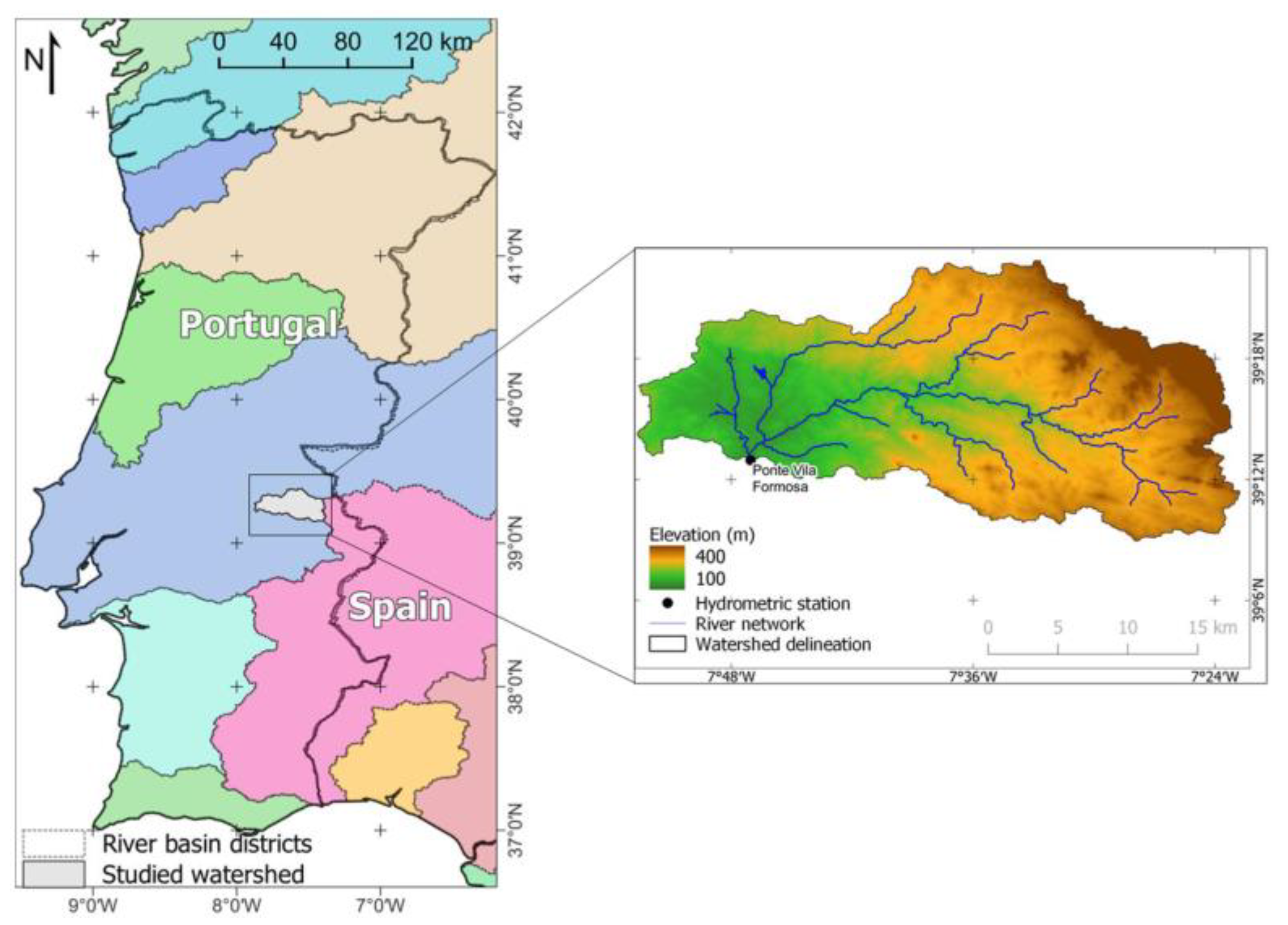
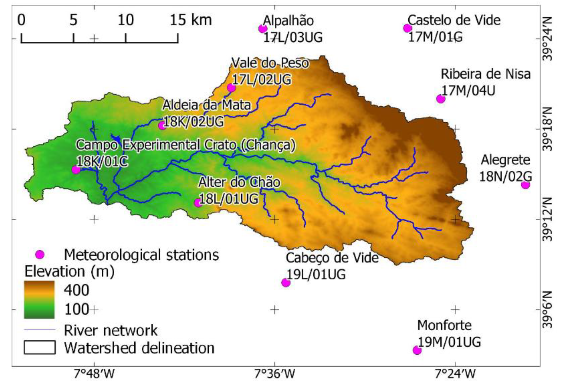
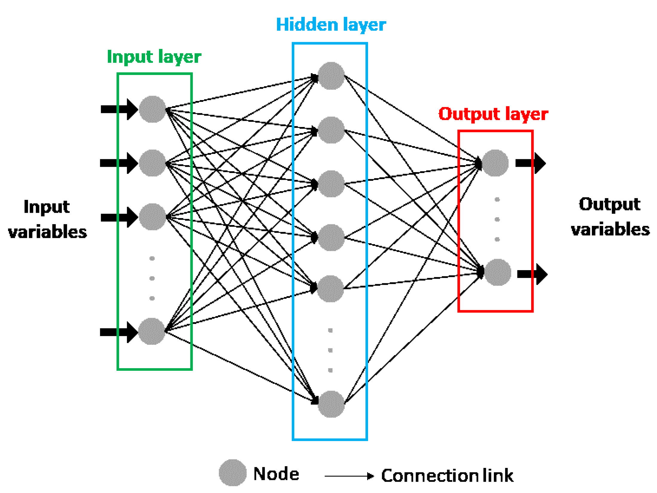
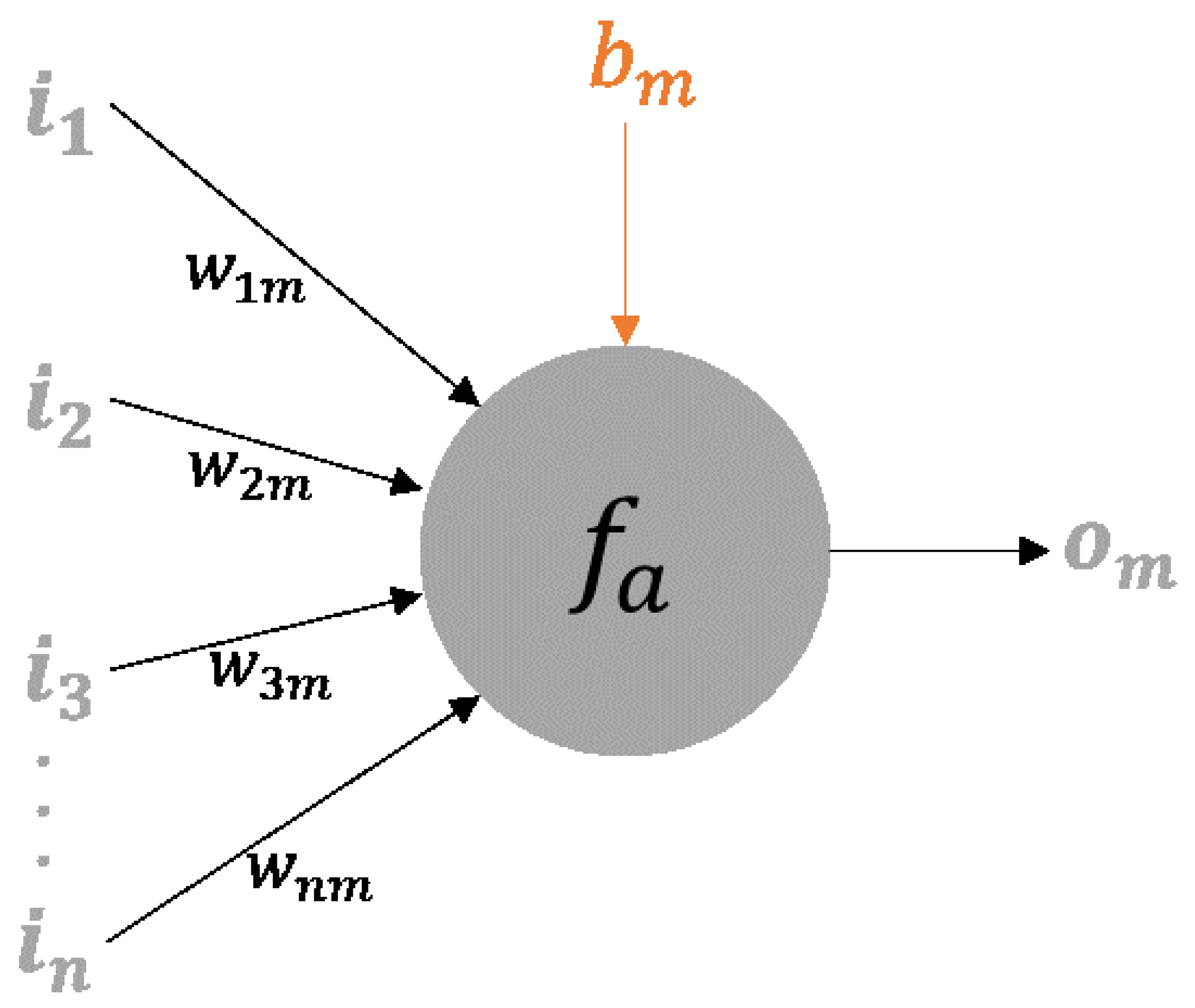
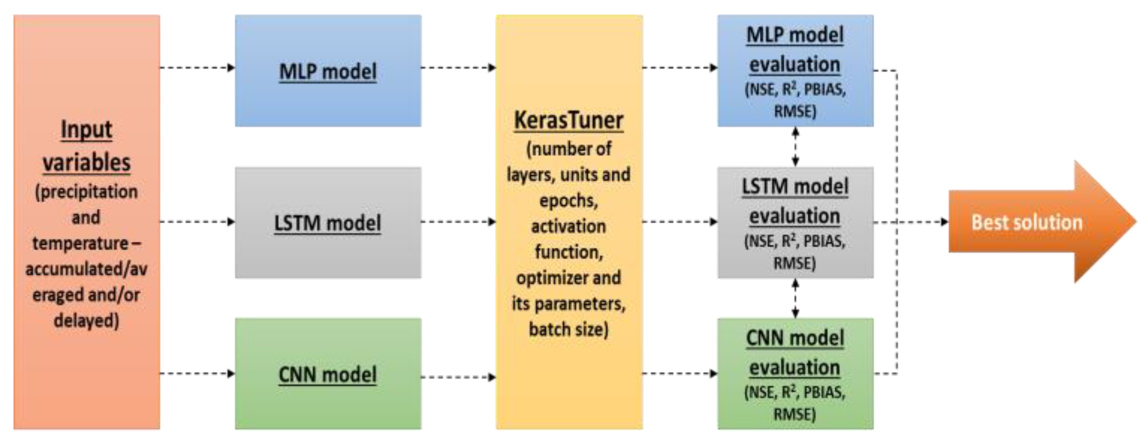
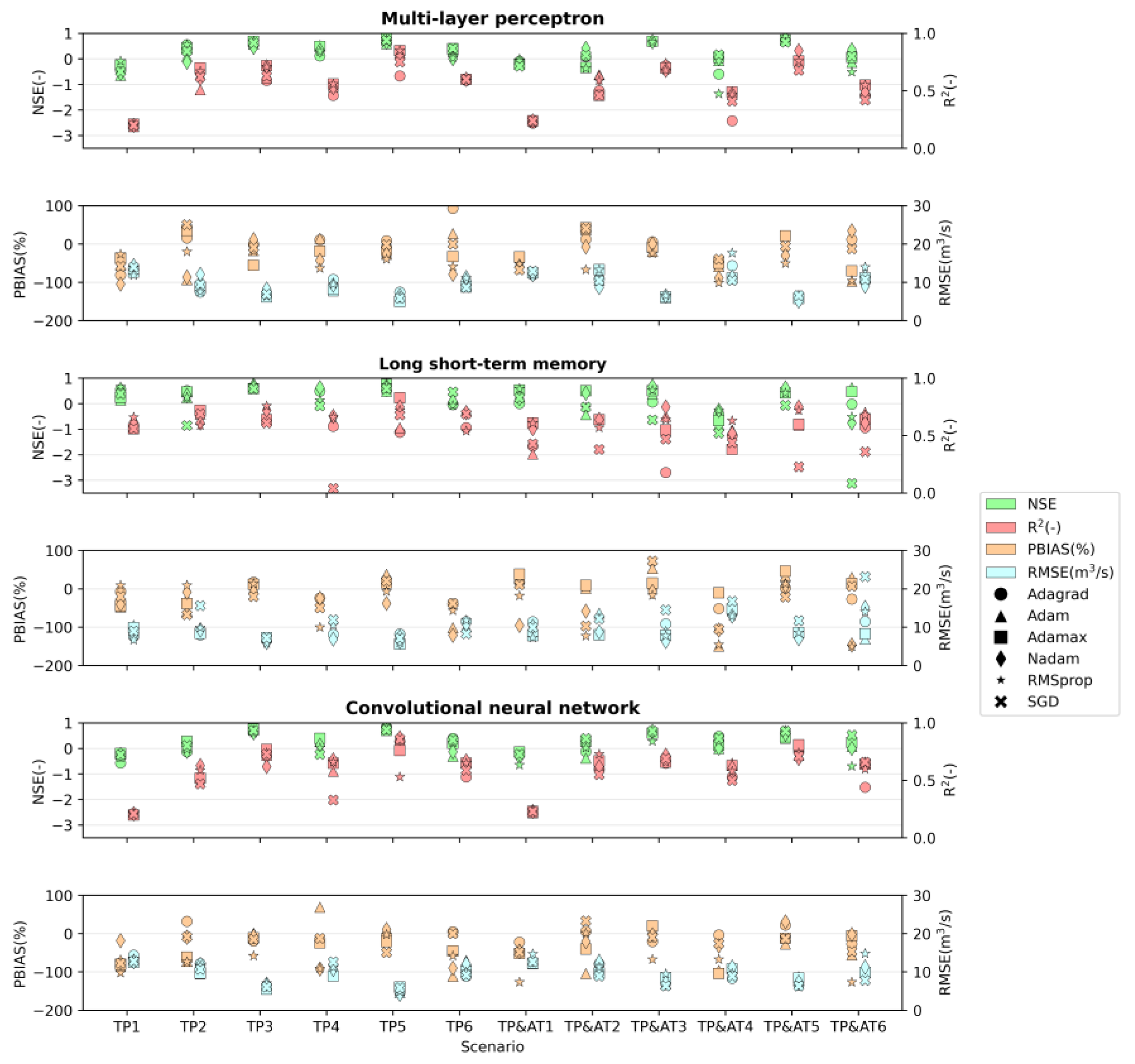
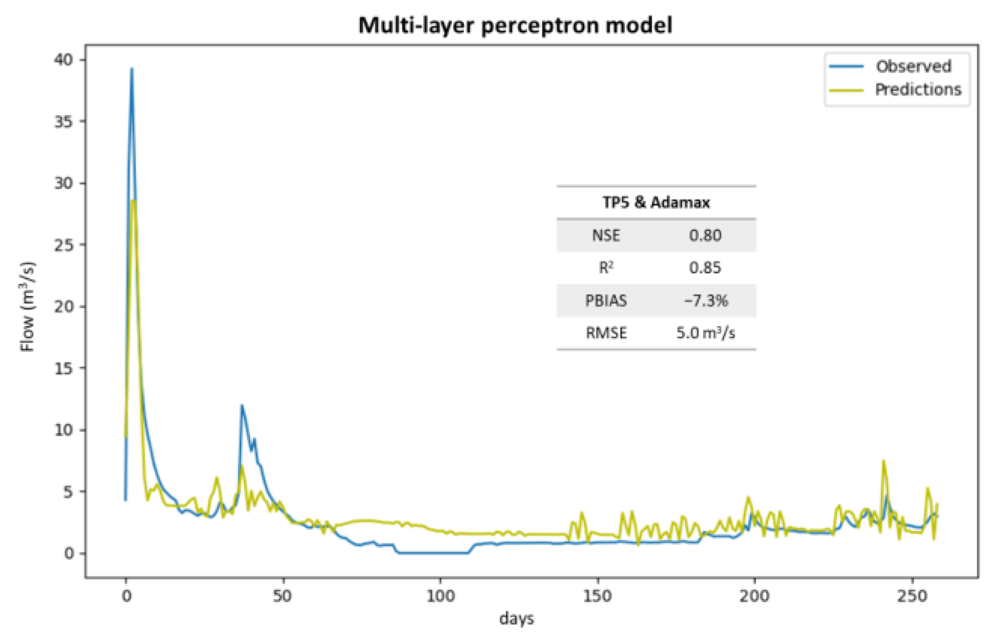
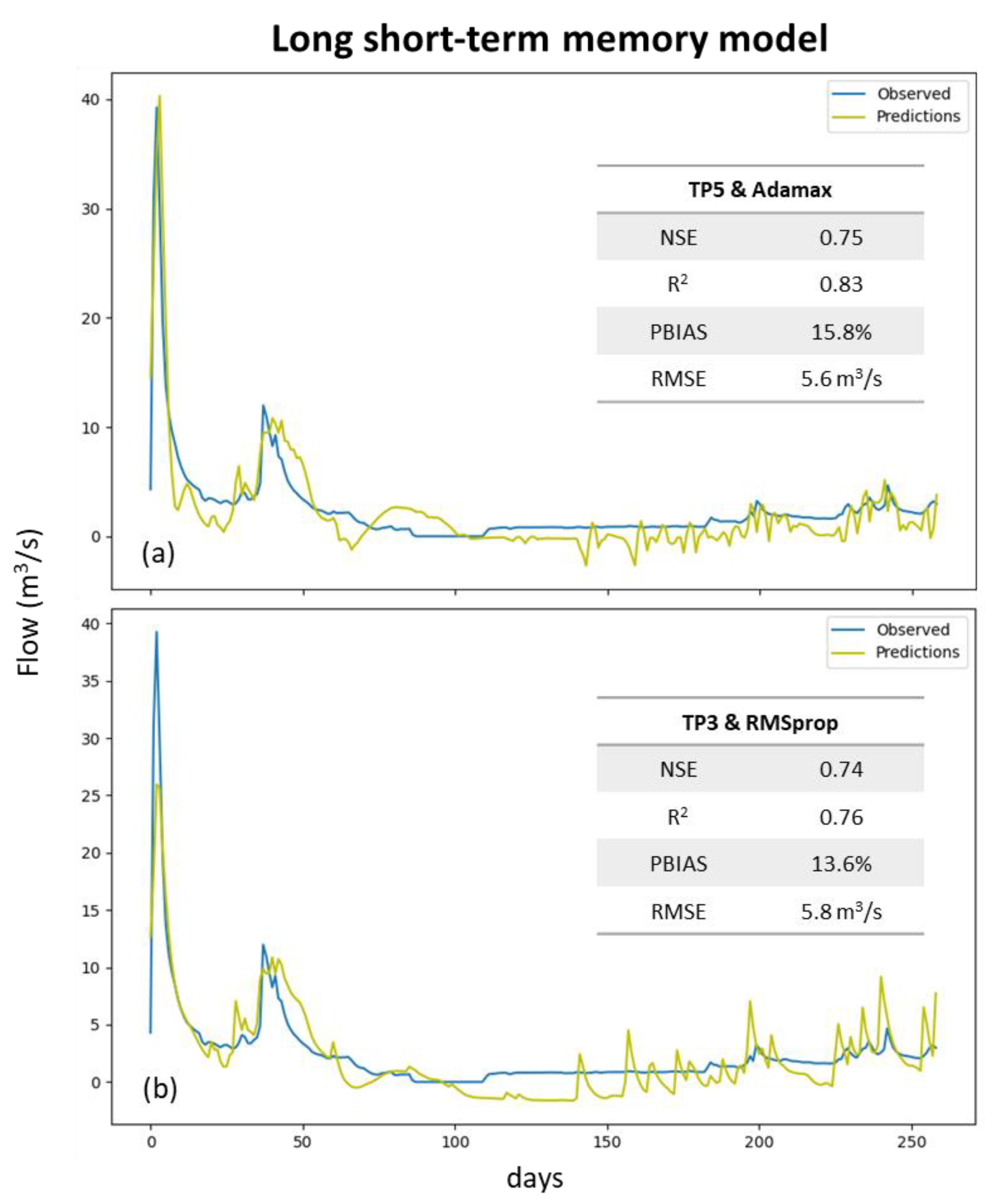
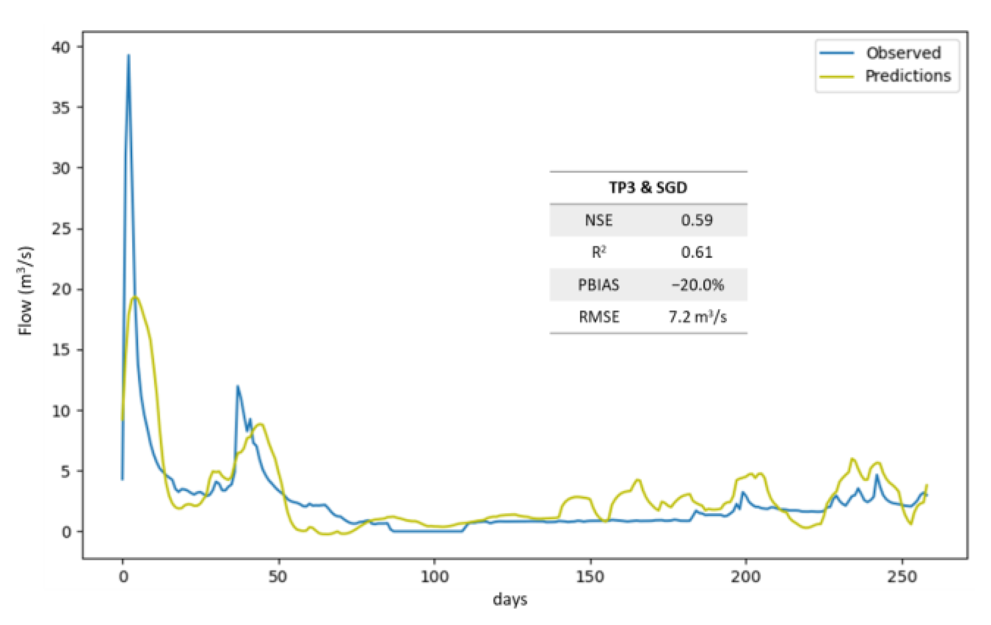
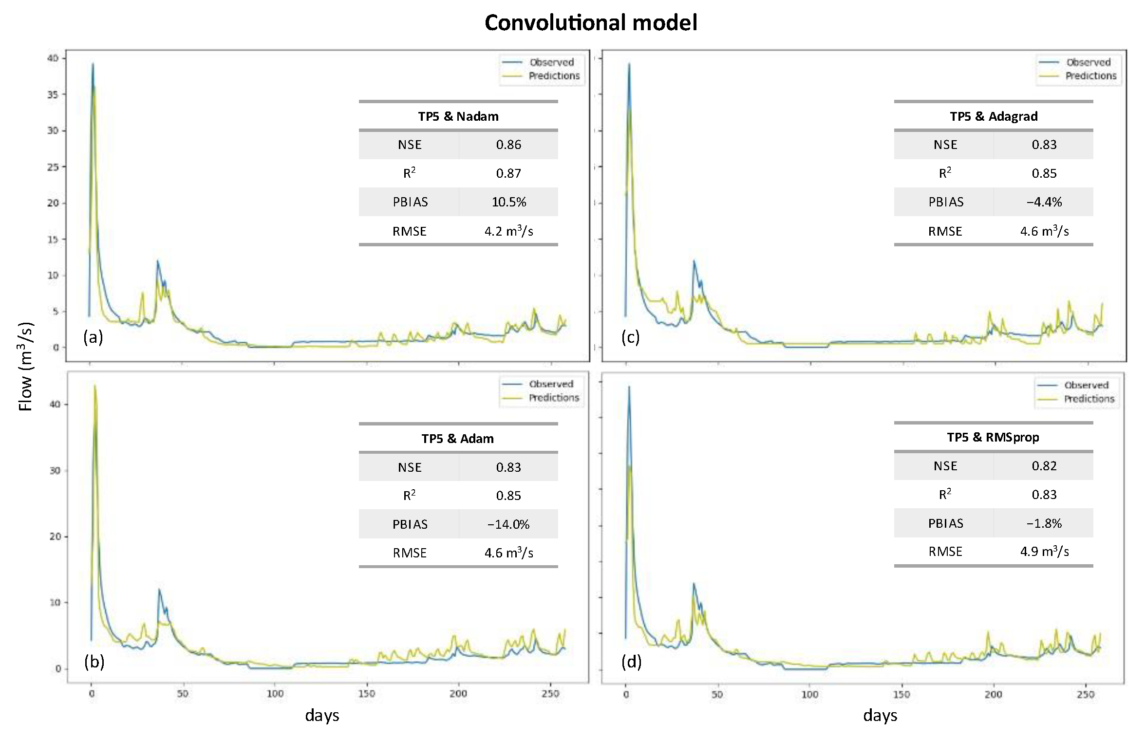
Table 1.
Average, minimum and maximum values, and number of completed years (total of daily values equals the number of days in the year) of annual precipitation registered in meteorological stations.
Table 1.
Average, minimum and maximum values, and number of completed years (total of daily values equals the number of days in the year) of annual precipitation registered in meteorological stations.
| Station | Period | Annual Precipitation | |||
|---|---|---|---|---|---|
| Average (mm) | Minimum (mm) | Maximum (mm) | Number of Completed Years | ||
| Aldeia da Mata | 1979–2021 | 621 | 374 | 1056 | 26 |
| Alegrete | 1980–2021 | 794 | 457 | 1269 | 17 |
| Alpalhão | 1979–2021 | 717 | 365 | 1224 | 26 |
| Alter do Chão | 2011–2021 | 614 | 101 | 1081 | 90 |
| Cabeço de Vide | 1931–2021 | 668 | 352 | 1184 | 68 |
| Campo Experimental Crato (Chança) | 1971–2021 | 662 | 323 | 973 | 29 |
| Castelo de Vide | 1931–2021 | 824 | 46 | 1555 | 76 |
| Monforte | 1911–2020 | 516 | 256 | 1030 | 88 |
| Ribeira de Nisa | 1979–1985 | 673 | 452 | 962 | 5 |
| Vale do Peso | 1931–2021 | 757 | 401 | 1324 | 77 |
Table 2.
Characterization of the streamflow dataset (average, minimum, maximum, and standard deviation values, and number of records) of Ponte Vila Formosa hydrometric station between 1 January 1979 and 30 May 2011 (entire dataset) and 25 July 2001 and 31 December 2008 (studied period) (source: SNIRH [22]).
| Period | Streamflow | ||||
|---|---|---|---|---|---|
| Average (m3 s−1) | Minimum (m3 s−1) | Maximum (m3 s−1) | Std. Deviation (m3 s−1) | Number of Records | |
| 1 November 1979–6 March 2019 | 3.8 | 0 | 272.8 | 12.7 | 7703 |
| 25 July 2001–31 December 2008 | 3.8 | 0 | 160.1 | 9.0 | 2645 |
Table 3.
Summary of Keras activation functions considered in the study.
| Long Name | Activation Name | Equation |
|---|---|---|
| Linear | linear | |
| Exponential linear unit | elu | |
| Rectified linear unit | relu | |
| Softsign | softsign | |
| Hyperbolic tangent | tanh |
Table 4.
Structure characteristics tested for MLP model.
| Layers | Number of Layers | Number of Neurons | Activation Function | Dropout after Dense | Dropout Rate |
|---|---|---|---|---|---|
| Input dense | 1 | 1, 2, 3, 4, 5, 6 or training set size | Linear, elu or relu | Yes/No | 0.1 or 0.2 |
| Hidden dense | 0, 1, 2, 3 or 4 | 1, 2, 3, 4, 5, 6 or training set size | Softsign, linear, elu or relu | Yes/No (one by each hidden layer) | 0.1 or 0.2 |
| Output dense | 1 | 1 | Softsign or linear | - | - |
Table 5.
Structure characteristics tested for the LSTM model, with ninput representing the number of neurons in the input layer.
Table 5.
Structure characteristics tested for the LSTM model, with ninput representing the number of neurons in the input layer.
| Layers | Number of Layers | Number of Neurons | Activation Function |
|---|---|---|---|
| Input LSTM | 1 | 4, 8, 16 or 32 | tanh (by default) |
| Hidden LSTM | 0, 2 or 4 | If hidden layers = 2: 1st layer: 2 × ninput 2nd layer: ninput If hidden layers = 4: 1st layer: 2 × ninput 2nd layer: 3 × ninput 3rd layer: 2 × ninput 4th layer: ninput | tanh (by default) |
| Output dense | 1 | 1 | linear |
Table 6.
Structure characteristics tested for the convolutional model.
| Layers | N. of Layers | N. of Filters | Kernel Size | Pooling Size | N. of Neurons | Activation Function | Dropout after Dense | Dropout Rate |
|---|---|---|---|---|---|---|---|---|
| Input convolutional | 1 | 8, 16, or 32 | 1, 5, or 10 | - | - | None (by default) | - | - |
| MaxPooling1D | 1 | - | - | 1 or 2 | - | - | - | - |
| Hidden convolutional | 0 or 1 | 8, 16, or 32 | 8, 16, or 32 | - | - | None (by default) | - | - |
| MaxPooling1D | 1 | - | - | 1 or 2 | - | - | - | - |
| Flatten | 1 | - | - | - | - | - | - | - |
| Hidden dense | 0, 1, or 2 | - | - | - | 3, 5, or 10 | softsign, linear, elu, or relu | Yes/No (one by each hidden layer) | 0.1 or 0.2 |
| Output dense | 1 | - | - | - | 1 | softsign, linear, elu, or relu | - | - |
Table 7.
Meteorological input data characterization (precipitation and air temperature, period 25 July 2001–31 December 2008).
Table 7.
Meteorological input data characterization (precipitation and air temperature, period 25 July 2001–31 December 2008).
| Meteorological Variable | Average | Minimum | Maximum | Std. Deviation |
|---|---|---|---|---|
| Daily total precipitation (mm) | 1.59 | 0 | 45.50 | 4.24 |
| Daily air temperature (°C) | 16.09 | 1.77 | 34.74 | 6.46 |
Table 8.
Tested scenarios and dataset dimensions (Acc. TP—accumulated days of total precipitation; Ave. AT—averaged days of air temperature).
Table 8.
Tested scenarios and dataset dimensions (Acc. TP—accumulated days of total precipitation; Ave. AT—averaged days of air temperature).
| Scenario | Total Precipitation (TP) or Total Precipitation + Air Temperature (TP&AT) | |||||
|---|---|---|---|---|---|---|
| Time Lag (Days) | Acc. TP (Days) | Ave. AT (Days) | Training Set Size | Validation Set Size | Test Set Size | |
| TP1 | - | 1 | - | 1851 | 529 | 265 |
| TP2 | - | 1,2,3,4,5,10 | - | 1845 | 527 | 264 |
| TP3 | - | 10,30,60 | - | 1810 | 517 | 259 |
| TP4 | 1,2,3,4,5,6,7 | - | - | 1846 | 527 | 265 |
| TP5 | 1,2,3,4,5,6,7 | 1,2,3,4,5,10 | - | 1810 | 517 | 259 |
| TP6 | 1,2,3,4,5,6,7 | 10,30,60 | - | 1845 | 527 | 264 |
| TP&AT1 | - | 1 | 1 | 1851 | 529 | 265 |
| TP&AT2 | - | 1,2,3,4,5,10 | 1,2,3,4,5,10 | 1845 | 527 | 264 |
| TP&AT3 | - | 10,30,60 | 10,30,60 | 1810 | 517 | 259 |
| TP&AT4 | 1,2,3,4,5,6,7 | - | - | 1846 | 527 | 265 |
| TP&AT5 | 1,2,3,4,5,6,7 | 1,2,3,4,5,10 | 1,2,3,4,5,10 | 1810 | 517 | 259 |
| TP&AT6 | 1,2,3,4,5,6,7 | 10,30,60 | 10,30,60 | 1845 | 527 | 264 |
Table 9.
Summary of hyper-parameters tuned for training algorithms.
| Training Algorithm | Hyper-Parameters Optimized | |
|---|---|---|
| Possible Values Tested for Learning Rate | Possible Values Tested for ε | |
| SGD | 1 × 10⁻⁴, 1 × 10⁻³ or 1 × 10⁻² | - |
| AdaGrad | - | 1 × 10⁻⁷ or 1 × 10⁻⁸ |
| RMSprop | - | |
| Adam | 1 × 10⁻⁴, 1 × 10⁻³ or 1 × 10⁻² | |
| AdaMax | ||
| Nadam | ||
Disclaimer/Publisher’s Note: The statements, opinions and data contained in all publications are solely those of the individual author(s) and contributor(s) and not of MDPI and/or the editor(s). MDPI and/or the editor(s) disclaim responsibility for any injury to people or property resulting from any ideas, methods, instructions or products referred to in the content. |
© 2023 by the authors. Licensee MDPI, Basel, Switzerland. This article is an open access article distributed under the terms and conditions of the Creative Commons Attribution (CC BY) license (https://creativecommons.org/licenses/by/4.0/).
Share and Cite
MDPI and ACS Style
Oliveira, A.R.; Ramos, T.B.; Neves, R. Streamflow Estimation in a Mediterranean Watershed Using Neural Network Models: A Detailed Description of the Implementation and Optimization. Water 2023, 15, 947. https://doi.org/10.3390/w15050947
AMA Style
Oliveira AR, Ramos TB, Neves R. Streamflow Estimation in a Mediterranean Watershed Using Neural Network Models: A Detailed Description of the Implementation and Optimization. Water. 2023; 15(5):947. https://doi.org/10.3390/w15050947
Chicago/Turabian StyleOliveira, Ana Ramos, Tiago Brito Ramos, and Ramiro Neves. 2023. "Streamflow Estimation in a Mediterranean Watershed Using Neural Network Models: A Detailed Description of the Implementation and Optimization" Water 15, no. 5: 947. https://doi.org/10.3390/w15050947
Note that from the first issue of 2016, this journal uses article numbers instead of page numbers. See further details here.