A Review of the Application of the Soil and Water Assessment Tool (SWAT) in Karst Watersheds

Abstract

Karst water resources represent a primary source of freshwater supply, accounting for nearly 25% of the global population water needs. Karst aquifers have complex recharge characteristics, storage patterns, and flow dynamics. They also face a looming stress of depletion and quality degradation due to natural and anthropogenic pressures. This prompted hydrogeologists to apply innovative numerical approaches to better understand the functioning of karst watersheds and support karst water resources management. The Soil and Water Assessment Tool (SWAT) is a semi-distributed hydrological model that has been used to simulate flow and water pollutant transport, among other applications, in basins including karst watersheds. Its source code has also been modified by adding distinctive karst features and subsurface hydrology models to more accurately represent the karst aquifer discharge components. This review summarizes and discusses the findings of 75 SWAT-based studies in watersheds that are at least partially characterized by karst geology, with a primary focus on the hydrological assessment in modified SWAT models. Different karst processes were successfully implemented in SWAT, including the recharge in the epikarst, flows of the conduit and matrix systems, interbasin groundwater flow, and allogenic recharge from sinkholes and sinking streams. Nonetheless, additional improvements to the existing SWAT codes are still needed to better reproduce the heterogeneity and non-linearity of karst flow and storage mechanisms in future research.

1. Introduction

Karst aquifers are an abundant source of water in many regions across the globe, providing freshwater supply to 20–25% of the world population [1] and upwards of 50% of the total drinking water supply in some countries [2]. They cover nearly 15.2% of Earth’s continental surface [3] and form by chemical dissolution of soluble carbonate rocks (i.e., limestone, dolomite, marble or evaporates) exerted by water enriched with carbon dioxide (CO₂) from the atmosphere or soil zone [4]. Depending on the degree of karstification, distinctive karst features can develop, including sinkholes and dolines, losing streams, springs, and vast networks of subsurface and hydrologically connected cracks, fissures, conduits, and caves [5].

1.1. Characteristics of Karst Systems

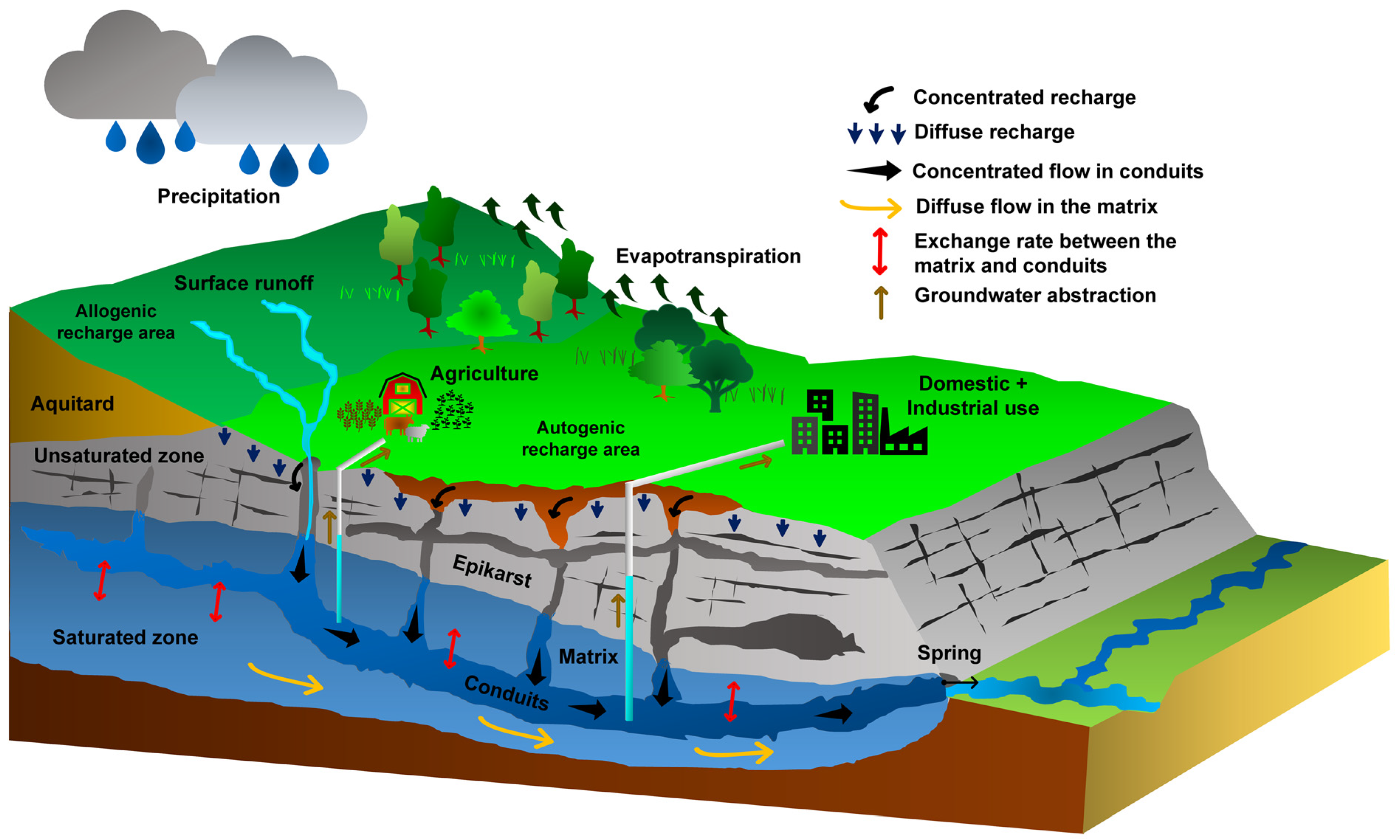
A karst system is generally composed of four main water-bearing mediums with distinct geomorphology, hydrodynamic properties, storage, and flow patterns: (1) the soil and non-karstic zone, (2) the epikarst, (3) the transmission zone—the latter three forming the unsaturated zone, and (4) the saturated zone [6]. These contrasting layers, which are interactively connected by water flow and solute transport, form the karstic critical zone [7,8].

Figure 1 shows a schematic model of a typical karst aquifer, including the surface hydrological processes and flow mechanisms of the underground karst subsystems. The epikarst represents a weathered horizon of a few meters above the vadose zone, with high permeability and porosity driven by the large supply of CO₂ that increases dissolution of carbonate rocks near the land surface. The epikarst, together with the soil cover, controls water infiltration, storage, temporal delay of recharge, and mixing processes. On the other hand, seasonal changes in surface temperature and vegetation cover substantially alter evapotranspiration and recharge, thus intensifying the variability of spring discharge and affecting the quality of the underground water resources [9,10,11]. Two recharge mechanisms are generally observed in a karst system: (1) diffuse recharge by slow percolation of infiltrated water from the epikarst to the saturated zone through low permeability small fissures in the vadose zone and (2) concentrated recharge via highly conductive karst features (enlarged fractures, sinkholes), allowing a fast transit of flow through the vadose zone to the saturated zone [12]. The transmission zone connects and transfers recharge water from the epikarst to the saturated zone where highly permeable karst conduits drain the fissured rock matrix, generating a flow to the groundwater discharge. Karst systems thus exhibit a duality of the storage and subsurface flow fields with (1) prolonged groundwater storage and low flow velocity/laminar flow in the matrix, and (2) low groundwater storage with rapid flow velocity/non-linear (turbulent) flow in the conduits. Dual discharge patterns to the aquifer outlet are also observed with (1) slow and continuous flow from the matrix during dry periods and (2) fast flow from the conduits during heavy rainfall events [6,13,14,15]. There is also limited karst hydrogeological research on the flow exchange mechanism between the conduit and the matrix, which primarily depends on the conduit properties and hydraulic head differences between the two mediums [16]. Internal runoff and infiltration provide autogenic recharge, whereas external runoff and sinking streams represent allogenic recharge from the neighboring areas [13]. Moreover, many karst watersheds are non-conservative (losing or gaining watersheds) due to interbasin groundwater flow (IGF) through their topographic divides. IGF may represent a substantial component of the streamflow where rivers traverse karst areas, thus affecting the catchment annual water balance. IGF is also not explicitly measurable, requiring the application of hydrogeochemical approaches based on major dissolved elements, isotopes, electrical conductivity, and water temperature monitoring or hydrogeological studies of groundwater flow paths [17].

Due to their intrinsic properties and complex hydrodynamic behavior, karst aquifers are vulnerable to contamination, overexploitation, and climate change [18,19]. In well-developed karst systems, natural processes such as absorption, degradation, and filtration are inefficient due to low storage capacity, fast water movement, short residence time, and limited interaction with the material of the aquifer. Contaminants can rapidly reach the groundwater table by concentrated recharge and propagate easily through karst conduits over large distances [20,21]. Moreover, climate change could result in more frequent and extended periods of high/transit or low groundwater levels [22]. Therefore, anticipating the impacts of climate change and anthropogenic hazards, and understanding the functioning of the karst aquifer water bearing components are compulsory tasks to safeguard these dwindling water supplies and set effective management schemes for karst water resources [23,24].

1.2. Numerical Modeling Approaches in Karst Hydrology

Hydrological models have become robust tools to simulate karst aquifer processes for a wide range of applications, which include integrated hydrodynamic analysis, modeling of karst hydrology, and forecasting of karst water resources availability under climate change [25]. These models can be classified into the following categories: the black box models, lumped models, and semi-distributed to distributed models.

Black box models use mathematical transfer functions or neural networks to relate the input rainfall signal to the output spring discharge without spatial information or an explicit representation of the watershed physical processes [26]. Thus, they may not be adequate to estimate future karst water resources over long time periods [23].

Lumped models conceptualize the physical processes at the scale of the entire hydrological system. They are generally used by modelers facing data scarcity problems [27]. Most lumped groundwater models adopt a series of linear or non-linear reservoirs to simulate the storage and flow components of the karst aquifer mediums, with parameters that represent the spatially averaged characteristics of the system [23].

In comparison to lumped models, the semi-distributed and distributed models explicitly represent the spatial variability of the watershed land and subsurface characteristics, boundary conditions, inputs, and hydrological processes [27]. Semi-distributed models could divide the catchment into hydrological response units (HRUs) and simulate the various hydrological processes in each HRU, use conceptual reservoirs to model areal recharge processes that lack spatial resolution, or represent the internal structure of a karst aquifer using pipe networks as conduit domains. On the other hand, fully-distributed models represent processes by discretizing the system in two- or three-dimensional grids and assigning parameters to each grid cell. In terms of karst hydrological modeling, the distributed karst models are subdivided into three categories: (1) the fully equivalent porous media approach, which uses average hydraulic properties over the aquifer area (concentrated fast flows and diffuse slow flows are not explicitly simulated), (2) the double continuum approach, which represents the matrix and karst conduits as two interacting continua with their hydraulic attributes, and (3) the combined discrete-continuum approach in which the karst conduits are embedded as discrete elements inside the matrix [26,27]. The use of distributed parameters models remains a challenge due to the complexity of karst aquifer mechanisms and the need for extensive hydrological and hydrogeological investigations to define the characteristics of the karst system (i.e., aquifer geometry, conduits network geometry and location, hydraulic properties and interactions between the matrix and conduits) [23,26].

1.3. Rationale of This Review of Karst Hydrological Modeling with SWAT

Improving the management and sustainability of karst groundwater resources remains a challenge. This is due to the limited understanding of the critical zone processes in karst watersheds across space and time, as well as the lack of research that characterizes the influence of vegetation cover, climate change, and anthropogenic activities on these processes [8,9]. Jeannin et al. [28] recently tested 13 karst numerical models in a karst watershed. The models consisted of lumped neural networks, reservoir models, and semi- to fully distributed models, and were compared for their performance efficiency in simulating groundwater recharge and karst spring hydrographs. The impact of the spatial distribution of recharge (land use, vegetation, precipitation) on the discharge was found to be low, as the semi- and fully distributed models had a comparable performance to the lumped reservoir models. The modelers stated, however, that the relative significance of the spatial distribution of the recharge function depends on the watershed characteristics. Other studies showed the substantial impact of vegetation and soil parameters (e.g., leaf area index, root depth, soil hydraulic conductivity and moisture content at saturation) on the evapotranspiration/infiltration and recharge functions in karst watersheds [29]. Sarrazin et al. [30] have found that karst recharge is not only sensitive to climatic factors but also to changes in land cover, using the large scale semi-distributed karst recharge model V2Karst V1.1. Bittner et al. [31] successfully simulated spring discharge in a karst watershed using the semi-distributed model Land use change modeling in KARSt systems (LuKARS). They validated the impact of land-use change on the spring water supply. Different techniques have also been developed to estimate evapotranspiration from remote sensing data and estimate groundwater recharge based on the reconstruction of distributed models of precipitation and evapotranspiration. These approaches were classified into four categories, namely: (1) the empirical direct methods, (2) the residual methods of the energy budget, (3) the deterministic methods, and (4) the vegetation index methods [32]. Ollivier et al. [33] established that incorporating the remote sensing-driven evapotranspiration model Simple Crop coefficient for Evapotranspiration (SimpKcET) into the grid-based distributed Karst Recharge and discharge Model (KaRaMel) improved the karst spring discharge simulations in low, intermediate, and high flow seasons, as well as the correlation between recharge events and recharge volumes. Yang et al. [34] also concluded that accounting for the heterogeneous spatial distribution of land cover and karst geological properties in a conceptually-based distributed karst hydrological model, referred to as the distributed karst Xinanjiang (DK-XAJ) model, improved the runoff simulation and the separation of groundwater recharge into rapid conduit flow and slow matrix flow.

As the need to predict future karst water resources under climate change projections and scenarios of land-use change increased, the use of the Soil and Water Assessment Tool (SWAT) in karst hydrological studies has gradually gained popularity. SWAT is a time-continuous, semi-distributed, process-based model that is widely used to simulate the spatial and temporal evolution of a catchment hydrological cycle, soil erosion and water quality, as well as the effects of land-use change and climate variability on catchment processes by dividing the watershed into subbasins and further into HRUs based on the land use, soil characteristics, and slope [35]. Numerous studies have directly applied the standard SWAT in karst basins, while others have modified its source code to improve the representation of karst hydrology by considering different karst flow regimes and features (e.g., sinkholes, springs, and IGF) [36]. Therefore, there exists a need for a comprehensive review on the applications of SWAT in karst watersheds in order to: (a) identify the areas of research in the water resource field in which SWAT was implemented in karstified watersheds, (b) investigate the different approaches in which karst processes were incorporated into SWAT, and (c) evaluate the modified SWAT models performance and adequacy in representing the heterogeneous and non-linear karst flow mechanisms.

1.4. Overview of Previous SWAT Applications and Modifications for Karst Modeling

The earliest SWAT studies in karst watersheds (a total of 4 articles) have been reported by Gassman et al. [37] as part of a full range review of research findings and methods for different application categories with SWAT (e.g., discharge, hydrological analyses, sensitivity analyses and calibration techniques, climate change impacts on hydrology, pollutant transport and fate). Their review was based on more than 250 SWAT articles identified in the literature up to the year 2007. Since then, the use of SWAT has seen a tremendous growth globally for a wide range of scales and complex environmental studies, with more than 5000 articles currently published in peer-reviewed journals [38]. The number of SWAT review studies has also expanded to cover a variety of applications, such as: SWAT developments in landscape representation, stream routing, and soil phosphorus dynamics [39], SWAT improvements in addressing environmental issues [40], quantification of ecosystem services [41], runoff simulation, hydrological impacts under changing environment, and non-point source pollution [42], SWAT limitations in simulating subdaily processes [43], methods used to develop a SWAT model at field-scale [44], SWAT simulations of hydro-climatic extremes [45], and SWAT applications in Mediterranean catchments [46], to name a few.

Despite these advancements, the numerical simulation of karst watersheds and their processes in SWAT is still underway. In fact, a recent research study by Eini et al. [36] cited only 36 articles describing SWAT-based applications in partially karstified and karst dominated watersheds, with just 13 studies featuring a modified SWAT code. To note, Eini et al. [36] did not provide a detailed overview of the karst modeling approaches adopted in articles that they cited but rather an introductory synopsis prior to presenting two modified SWAT codes that they developed and applied in a karst watershed. Therefore, our paper is the first—to our best knowledge—to present an in-depth review of the studies conducted with SWAT in karst watersheds, building on the selected list of publications by Eini et al. [36] and extending to the full range of studies between the years 2000–2022. The objectives of our present review are to: (a) describe the SWAT subroutines that correspond to the different processes driving the flow of water in the critical zone (i.e., surface runoff, evapotranspiration, infiltration, interflow, recharge, baseflow), (b) summarize and discuss the research methods and findings for the standard and modified SWAT models in karst influenced watersheds, (c) identify potential constraints of the existing SWAT modeling approaches in representing the heterogeneous and non-linear flow mechanisms in karst aquifers, and (d) propose future research directions in order to enhance the applicability of SWAT in karst watersheds and the reliability assessment of karst water resources for future management and planning.

This review will present the different applications of SWAT (i.e., water quantity and quality, land-use and climate change, erosion processes, ecohydrological assessment, and water resources management) in karst influenced and karst dominated watersheds. However, the primary focus of the discussion will be the hydrological assessment in the SWAT applications that featured SWAT coupling with other hydrological models or modifications to the SWAT recharge and groundwater flow equations. These studies aimed to improve the representation of karst features, baseflow, and peak flows in SWAT prior to simulating other watershed processes, such as sediment or pollutant transport.

2. Equations in SWAT for Hydrological Simulation

SWAT is a continuous-time semi-distributed agro-eco-hydrological model developed by the United States Department of Agriculture (USDA) [47]. The model has been successfully applied to monitor and predict the impacts of environmental and anthropogenic changes on the physical processes in watersheds at small, regional, and subcontinental scales (e.g., [48,49,50,51,52,53,54,55,56,57]). SWAT uses meteorological data, i.e., precipitation, air temperature, relative humidity, wind speed, and solar radiation, in addition to topography, soil properties, and land-use data, to simulate the watershed water balance components at different time steps (subdaily to annual). It can also model water quality and soil erosion [43,58]. The watershed is first disaggregated into subbasins connected through a stream channel and further into HRUs that represent areas of homogenous land use, soil, and slope properties [59]. The definition of HRUs is performed using a geographic information system (GIS), such as the ArcSWAT interface of ArcGIS or the QSWAT plugin of QGIS, coupled to the SWAT model to integrate the topographic, soil, and land-use inputs [60]. The simulated catchment processes in SWAT include surface runoff, infiltration, evapotranspiration, lateral flow, tile drainage, percolation, water stored in the soil profile, return flow from unconfined aquifers, consumptive water use through pumping (if any), recharge from surface water bodies, and in-stream processes, such as channel routing (main and tributary) and transformation of nutrients and pesticides [61]. These components are represented in each HRU by five storage volumes, namely the canopy interception, snow pack, soil profile, shallow aquifer, and deep aquifer [62].

Watershed hydrology in SWAT is represented by a land phase and a routing phase, whereby runoff, sediments, and agricultural chemical yields from all subbasin HRUs are aggregated to the main reach of the subbasin and routed rough the channel network to the outlet(s) of the main catchment [63]. The fundamental daily water balance equation used in SWAT to represent the land phase of the hydrological cycle is given as follows [64]:

$$S{W}_t-S{W}_0={{\displaystyle \sum }}_{i=1}^t\left(P_{day}-Q_{surf}-E{T}_a-W_{seep}-Q_{gw}\right)$$

(1)

where $S{W}_0$ and $S{W}_t$ are the initial and final soil water content of the entire soil profile for the simulation period, respectively, $P_{day}$, $Q_{surf}$, $E{T}_a$, $W_{seep}$, and $Q_{gw}$ are precipitation, surface runoff, actual evapotranspiration, percolation and bypass flow exiting the soil bottom to the vadose zone, and return flow, respectively (all variables are expressed in mm H₂O.day⁻¹).

SWAT offers different options to simulate scheduled irrigation and auto-irrigation of crops. The auto-irrigation approach is generally used when irrigation scheduling data are lacking. Auto-irrigation is triggered by two stress identifiers: (1) plant water stress, whereby irrigation is applied to meet the plant water demand if the ratio of actual transpiration to potential transpiration falls below a user-specified threshold, and (2) soil water deficit, whereby irrigation is applied if the water content in the soil profile drops below field capacity by more than a user-defined soil water depletion threshold [65]. Sources of irrigation include river reaches, reservoirs, shallow and deep aquifers, or a source from outside the watershed, and irrigation demand is met based on the source water availability [66]. When irrigation is applied, the SWAT water balance is adjusted as follows:

$$S{W}_t-S{W}_0={{\displaystyle \sum }}_{i=1}^t\left(P+Irr\right)-{{\displaystyle \sum }}_{i=1}^t\left(Q_{surf}-E{T}_a-W_{seep}-Q_{gw}\right)$$

(2)

where $S{W}_0$ and $S{W}_t$ are the initial and the final soil water content of the entire soil profile for the simulation period, $P$, $Irr$, $Q_{surf}$, $E{T}_a$, $W_{seep}$, and $Q_{gw}$ represent precipitation, irrigation, surface runoff, actual evapotranspiration, percolation and bypass flow exiting the soil bottom to the vadose zone, and return flow, respectively (all variables are expressed in mm H₂O.day⁻¹).

Water routed through channels to the main watershed outlets is generated from direct surface runoff, lateral soil flow, baseflow from groundwater storage, and tile flow [67]. These flow components contribute to the catchment water yield, which is considered a critical parameter in the sustainable management of water resources [68]. Hence, water yield is defined as the net water volume leaving the HRU and entering a reach at the subbasin level into the main channel, as follows:

$$WYLD=Q_{surf}+Q_{lat}+Q_{gw}+Q_{tile}-T_{loss}$$

(3)

where $WYLD$ is the water yield, $Q_{surf}$, $Q_{lat}$, and $Q_{gw}$ are the surface runoff, soil lateral flow, and return flow from the shallow aquifer to the main channel, respectively, $Q_{tile}$ is the tile flow, and $T_{loss}$ represents the losses from the tributary in the HRU via transmission through the riverbed (all variables are expressed in mm H₂O.day⁻¹).

The governing equations of the watershed hydrological components are presented thoroughly in the theoretical documentation of SWAT [69]. Hence, the primary focus in Section 2.1 and Section 2.2 below was devoted to flow processes in the critical zone that directly impact streamflow simulation in standard SWAT. These processes were grouped under: (1) surface water hydrology (Section 2.1) and (2) subsurface water hydrology (Section 2.2). A set of equations that are fundamental in hydrological modeling with SWAT were provided in each subsection, with a corresponding list of SWAT variables in Appendix A (

Table A1. List of SWAT Variables in the Main Text.

Variable	Definition
$SW$	Soil water content
$P$	Precipitation
$Q_{surf}$	Surface runoff
$PET$	Potential evapotranspiration
$E{T}_a$	Actual evapotranspiration
$W_{seep}$	Percolation and bypass flow drained from the soil profile
$Q_{gw}$	Return flow
$Q_{lat}$	Soil lateral flow
$Q_{tile}$	Tile flow
$T_{loss}$	Channel transmission losses
$WYLD$	Water yield
$Irr$	Irrigation
$LAI$	Lead area index
$\lambda$	Latent heat of vaporization
$E$	Depth rate evaporation
$\mathrm{\Delta }$	Slope of the saturation vapor pressure–temperature curve
$H_{net}$	Net radiation
$G$	Heat flux density to the ground
${\rho }_{air}$	Air density
$c_p$	Specific heat at constant pressure
$e_z^0$	Saturation vapor pressure of air at height z
$e_z$	Water vapor pressure of air at height z
$\gamma$	Psychometric constant
$r_c$	Plant canopy resistance
$r_a$	Aerodynamic resistance
$S$	Soil moisture retention parameter
$CN$	Curve number
$I_a$	Initial water abstraction prior to runoff
$I\left(t\right)$	Infiltration
$I_{acc}\left(t\right)$	Cumulative infiltration after ponding
$\psi$	Wetting front matric potential
$\mathrm{\Delta }\theta$	Change in soil moisture content
$K_e$	Effective hydraulic conductivity
$q_{peak}$	Peak runoff rate
${\alpha }_{tc}$	Fraction of daily rainfall during the time of concentration
$A$	Subbasin area
$t_{conc}$	Time of concentration for the subbasin
$K_{ch}$	Effective hydraulic conductivity of the channel alluvium
$L_{ch }$	Channel length
$P_{ch}$	Wetted perimeter in the channel
$TT$	Flow travel time
$K_{sat}$	Saturated hydraulic conductivity
$SAT$	Saturation water content
$FC$	Field capacity water content
$W_{perc,ly}$	Water percolation to an underlying soil layer
$W_{perc,ly=n}$	Water percolating out of the lowest soil layer
$S{W}_{ly,excess}$	Drainable volume of water in the soil layer
$T{T}_{perc}$	Travel time through the soil layer
$W_{crk,btm}$	Crack flow past the lower boundary of the soil profile
$crk$	Total crack volume for the soil profile
$cr{k}_{ly=nn}$	Crack volume for the deepest soil layer
$dept{h}_{ly=nn}$	Depth of the deepest soil layer
$slp$	Increase in elevation per unit distance
${\varnothing }_d$	Drainable (residual) porosity of the soil layer
$L_{hill}$	Hillslope length
$E_{e,ly}$	Evaporation drawn from the soil layer
$E_{t,ly}$	Transpiration drawn from the soil layer
${\delta }_{gw}$	Delay time for recharge to reach the aquifers
$W_{rchrg}$	Recharge to the aquifers
$W_{rchrg,sh}$	Recharge to the shallow aquifer
$W_{rchrg,dp}$	Recharge to the deep aquifer
$Q_{gw,sh}$	Return flow from the shallow aquifer
$Q_{gw,dp}$	Groundwater flow from the deep aquifer
${\alpha }_{gw,sh}$	Groundwater recession constant of the shallow aquifer
${\alpha }_{gw,dp}$	Groundwater recession constant of the deep aquifer
${\beta }_{dp}$	Coefficient of percolation to the deep aquifer
$a{q}_{sh}$	Water level in the shallow aquifer
$a{q}_{shthr,q}$	Threshold water level in the shallow aquifer for return flow
$E{T}_{rvp}$	Actual groundwater evapotranspiration by plant uptake/capillary rise
$E{T}_{rvp,max}$	Maximum water removed from the shallow aquifer
${\beta }_{rvp}$	Groundwater evaporation coefficient
$a{q}_{shthr,rvp}$	Threshold water level in the shallow aquifer for groundwater evaporation to occur
$Q_{pump,sh}$	Water withdrawn by pumping from the shallow aquifer
$V_{seep}$	Seepage from the pond or wetland
$A_{wet}$	Water surface area of the pond or wetland
$V_{seep,pot}$	Seepage from a pothole
$SA$	Pothole surface area

). These equations serve to help the reader understand the methods used in SWAT to simulate surface and groundwater flows, prior to discussing the modifications made to the SWAT source code for the different applications in the realm of karst hydrology (Section 4 of the review).

2.1. Surface Water Hydrology

2.1.1. Evapotranspiration

SWAT provides three methods to simulate daily potential evapotranspiration (PET) at the HRU scale, namely the Penman-Monteith [70], the Priestley-Taylor [71], and the Hargreaves methods [72]. Between the three approaches, the Penman-Monteith equation is considered the most suited to estimate PET, as it explicitly separates the effects of climate and land cover properties on each of the evapotranspiration components [30,33]. This method is represented with Equation (4), as follows [69]:

$$\lambda E=\frac{\mathrm{\Delta }\left(H_{net}-G\right)+{\rho }_{air}\times c_p\left(e_z^0-e_z\right)/r_a}{\mathrm{\Delta }+\gamma \left(1+r_c/r_a\right)}$$

(4)

where $\lambda E$ is the latent heat flux density (MJ.m⁻².day⁻¹), $\lambda$ is the latent heat of vaporization (MJ.kg⁻¹), $E$ is the depth rate evaporation (mm.day⁻¹), $\mathrm{\Delta }$ is the slope of the saturation vapor pressure–temperature curve (de/dT) (kPa.°C⁻¹), $H_{net}$ is the net radiation (MJ.m⁻².day⁻¹), $G$ is the heat flux density to the ground (MJ.m⁻².day⁻¹), ${\rho }_{air}$ is the air density (kg.m⁻³), $c_p$ is the specific heat at constant pressure (MJ.kg⁻¹.C⁻¹), $e_z^0$is the saturation vapor pressure of air at height z (kPa), $e_z$is the water vapor pressure of air at height z (kPa), $\gamma$ is the psychometric constant (kPa.°C⁻¹), $r_c$is the plant canopy resistance (s.m⁻¹), and $r_a$ is the diffusion resistance of the air layer (aerodynamic resistance) (s.m⁻¹).

PET in SWAT depends on plant growth, which considers canopy resistance expressed as a function of the minimum effective stomatal resistance for a single leaf and the leaf area index (LAI). The LAI, defined as one half the total leaf area per unit ground area, reflects the structural characteristics of the plant canopy and defines the size of the interface for energy and mass exchanges between the vegetation surface and the atmosphere [73]. Evapotranspiration is also related to the canopy height required to determine the aerodynamic resistance parameter [69].

SWAT uses the LAI in conjunction with a simplified version of the Environmental Policy Integrated Climate (EPIC) plant growth model to simulate the phenological development of plants and estimate evapotranspiration [74]. In addition to the LAI development, the plant growth module of SWAT includes the simulation of the light interception and the conversion of intercepted light into biomass, assuming a plant species-specific radiation-use efficiency [75]. Plant development is primarily dependent on the base temperature for growth derived from minimum, maximum, and optimum temperature requirements. The plants heat unit requirements are quantified and related to the time of planting and maturity [76]. The LAI is incremented daily based on the accumulated potential heat units. It first increases to a crop-specific maximum value, remains constant until the senescence stage, then decreases linearly to zero at harvest. Similarly, the canopy height increases until a crop-specific maximum is achieved and stays at this height through the remainder of the growing season [77]. The potential crop leaf growth and biomass are first computed under optimal conditions and further adjusted for actual growth under stress factors such as water, temperature, and nutrients [78]. SWAT also uses dormancy in function of day length and latitude to repeat the annual growth cycle for trees and perennials [73].

After estimating potential evapotranspiration, SWAT calculates actual evapotranspiration (ETa), which includes four components: the canopy evaporation, the plant transpiration, the sublimation and soil surface evaporation, and the groundwater evapotranspiration [79]. The model first evaporates any precipitation intercepted by the plant canopy. Then, actual plant transpiration is estimated as a function of the potential transpiration adjusted for the wet canopy storage, root depth, soil water content, and the leaf area index, which depends on the plant developmental stage. Soil evaporation is modeled as a function of potential evapotranspiration adjusted for canopy evaporation and the rate of shading. If snow is present in the HRUs, sublimation takes place until evaporation from soil could occur after snow melting. Subsequently, SWAT proceeds to adjust the maximum possible soil evaporation for plant water use and partitions the evaporative demand between the different soil layers, in order to estimate the actual evaporation at each layer based on the soil water content [74,79,80].

2.1.2. Surface Runoff and Infiltration

In SWAT, soil surface runoff and infiltration are estimated from precipitation by one of the following two approaches: (1) the modified Soil Conservation Service Curve Number (SCS-CN) procedure and (2) the Green and Ampt Mein Larson (GAML) excess rainfall method. The SCS-CN approach simulates cumulative surface runoff based on cumulative precipitation and soil retention properties for daily time step, whereas the GAML approach simulates surface runoff for subdaily time step applications using subdaily precipitation input data [45,81,82].

Surface runoff is estimated with the SCN-CN procedure as follows [66]:

$$Q_{surf}=\frac{{\left(P-I_a\right)}^2}{\left(P-I_a\right)+S}\hspace{1em}when P>I_a; else Q_{surf}=0$$

(5)

where $Q_{surf}$ is the accumulated runoff, $P$ is the total precipitation, $I_a$ is the initial water abstraction prior to runoff due to surface storage interception and infiltration (generally approximated as $0.2S$, but can vary with the soil type), and S is the soil moisture retention parameter (all variables are expressed in mm H₂O.day⁻¹).

The soil retention parameter (S) varies temporally with the changes in moisture content, and spatially in function of the soil type, land use, and management practices. It can also be assumed to vary with the accumulated plant evapotranspiration. The retention parameter is expressed as a function of the daily curve number (CN) of the Antecedent Moisture Condition-II (AMC-II) for a given land use/cover and hydrological soil group as follows [66]:

$$S=\frac{25,400}{CN}-254$$

(6)

The SCS approach defines three antecedent moisture conditions, namely AMC-I for dry/wilting point condition, AMC-II for average moisture, and AMC-III wet/field capacity, represented by curve numbers CN1, CN2 and CN3, respectively. CN1 and CN3 are computed as a function of CN2 as follows:

$$CN1=CN2-\frac{20\left(100-CN2\right)}{\left(100-CN2+e^{2.533-0.0636\left(100-CN2\right)}\right)}$$

(7)

$$CN3=CN2\times e^{0.000673\left(100-\mathrm{CN}2\right)}$$

(8)

Infiltration rate is calculated using the GAML equation as follows [83]:

$$I\left(t\right)=K_e\left(1+\frac{\psi \times \mathrm{\Delta }\theta }{I_{acc}\left(t\right)}\right)$$

(9)

where $I\left(t\right)$ is the infiltration rate (mm H₂O) at the simulation time step $t$ (subdaily), $K_e$ is the effective hydraulic conductivity, which considers soil water content and land-use impact as a function of CN (mm.h⁻¹), $\psi$ is the wetting front matric potential (mm), $\mathrm{\Delta }\theta$ is the change in soil moisture content (mm.mm⁻¹), and $I_{acc}\left(t\right)$ is the cumulative infiltration after ponding (mm H₂O.hour⁻¹). The cumulative depth of water infiltration $I_{acc}\left(t\right)$ is computed as follows:

$$I_{acc}\left(t\right)=I_{acc}\left(t-1\right)+K_e\times \mathrm{\Delta }\mathrm{t}-\psi \times \mathrm{\Delta }\theta \times ln\left[\frac{I_{acc}\left(t\right)+\psi \times \mathrm{\Delta }\theta }{I_{acc}\left(t-1\right)+\psi \times \mathrm{\Delta }\theta }\right]$$

(10)

where $t-1$ is the previous simulation time step. Equation (10) is solved using a successive substitution technique. Subsequently, the infiltration rate is calculated using Equation (9) for each time step. Surface runoff is generated when the rainfall intensity exceeds infiltration rate. Otherwise, the total rainfall volume during the time step infiltrates into the soil.

2.1.3. Channel Flow and Flow Routing

For stream channel routing, Manning’s equation is used to calculate the rate and velocity of flow in the reach of each subbasin when the streamflow is less than the bankfull discharge rate, computed as a function of the bankfull channel width and depth. SWAT incorporates floodplain inundation geometry into the channel routing simulation if the streamflow is greater than bankfull flow [84].

The peak runoff rate, reached when all the subbasins are contributing to flow at the outlet, is estimated using the modified rational method, as follows [85]:

$$q_{peak}=\frac{{\alpha }_{tc}\times Q_{surf}\times A}{3.6\times t_{conc}}$$

(11)

where $q_{peak}$ is the peak runoff rate (m³.s⁻¹), ${\alpha }_{tc}$ is the fraction of daily rainfall that occurs during the time of concentration, $Q_{surf}$ is the surface runoff (mm H₂O.day⁻¹), $A$ is the subbasin area (km²), and $t_{conc}$ is the time of concentration for the subbasin (hours), calculated as the sum of the overland flow time and channel flow time. Water is routed through the channel network using either the Muskingum routing method (based on the continuity and empirical linear storage equations) [86] or the variable storage routing method (based on the continuity equation) [87,88].

Water transmission losses can occur through the side and bottom of the river channels and enter the bank storage or the deep aquifer. Transmission losses are estimated as follows [89]:

$$T_{loss}=K_{ch}\times L_{ch }\times P_{ch}\times TT$$

(12)

where $T_{loss}$ represents the channel transmission losses (m³ H₂O), $K_{ch}$ is the effective hydraulic conductivity of the channel alluvium (mm.h⁻¹), $L_{ch }$is the channel length (km), $P_{ch}$ is the wetted perimeter in the channel (m), and $TT$ is the flow travel time (hours).

2.2. Subsurface Water Hydrology

2.2.1. Soil Water Percolation and Lateral Flow

The water percolation component in SWAT redistributes infiltrated water in the soil profile using a storage routing method combined with an optional crack-flow routine. Percolation is simulated when the water content of a soil layer exceeds its field capacity defined as the sum of the available soil water content and permanent wilting point. Percolated water moves to the subsequent layer unless it is saturated, frozen, or impervious [90,91,92]. Water percolation is estimated as follows:

$$W_{perc,ly}=S{W}_{ly,excess}\left(1-e^{\frac{-\mathrm{\Delta }t}{T{T}_{perc,ly}}}\right)$$

(13)

where $W_{perc,ly}$ is the water percolating from soil layer ($ly$) to the underlying soil layer (mm H₂O.day⁻¹), $S{W}_{ly,excess}$ is the drainable volume of water in the soil layer ($ly$) on a given day (computed as the difference between the water content of the soil layer and field capacity, in mm H₂O.day⁻¹), $\mathrm{\Delta }t$ is the length of the time step (hours), and $T{T}_{perc,ly}$ is the travel time through the soil layer (hours), calculated as follows:

$$T{T}_{perc,ly}=\frac{SA{T}_{ly}-F{C}_{ly}}{K_{sat,ly}}$$

(14)

where $K_{sat,ly}$(mm.h⁻¹), $SA{T}_{ly}$ (mm H₂O), and $F{C}_{ly}$ (mm H₂O) represent the saturated hydraulic conductivity, saturation water content, and field capacity water content of the soil layer $\left(ly\right)$, respectively.

SWAT incorporates a crack flow module that can be used to simulate bypass (crack) or preferential flow in the soil. The use of the crack flow approach to increase infiltration rates from the surface is optional and requires the activation of a crack flow code by the user [36]. Crack volume for each soil layer is modeled in the dry seasons, which allows infiltrated rainwater to move rapidly through the soil profile along vertical cracks, and disappears in wet conditions [93]. Bypass flow from the bottom of the soil profile to the saturated zone is computed using Equation (15), and excess water that leaves the bottom of the soil profile through the vadose zone is calculated by combining percolation and bypass flow, as shown in Equation (16) [69]:

$$W_{crk,btm}=0.5\times crk\left(\frac{ cr{k}_{ly=nn}}{ dept{h}_{ly=nn}}\right)$$

(15)

$$W_{seep}=W_{perc,ly=n}+W_{crk,btm}$$

(16)

where $W_{perc,ly=n}$ is the water percolating out of the lowest soil layer,$W_{crk,btm}$ is the crack flow past the lower boundary of the soil profile (mm H₂O.day⁻¹), $crk$ is the total crack volume for the soil profile on a given day (mm), $cr{k}_{ly=nn}$ is the crack volume for the deepest soil layer on a given day (mm), $dept{h}_{ly=nn}$is the depth of the deepest soil layer (mm), and $W_{seep}$ is the total volume of water drained from the bottom of the soil profile (mm H₂O.day⁻¹).

Lateral flow (soil interflow) along a steep hillslope is computed simultaneously with percolation when the soil water content exceeds its field capacity. It is simulated using a kinematic storage routing method (Equation (17)) that is based the on slope, slope length, and saturated conductivity of each soil layer [63,92], as follows:

$$Q_{lat}=0.024\left(\frac{2\times S{W}_{ly,excess}\times K_{sat}\times slp}{{\varnothing }_d\times L_{hill}}\right)$$

(17)

where $Q_{lat}$ is the daily water flux from the hillslope outlet (mm H₂O.day⁻¹), $S{W}_{ly,excess}$ is the drainable volume of water stored in the saturated zone of the hillslope per unit area (mm H₂O), $K_{sat}$ is the saturated hydraulic conductivity of the soil (mm.h⁻¹), $slp$ is the increase in elevation per unit distance, ${\varnothing }_d$ is the drainable (residual) porosity of the soil layer (mm/mm), and $L_{hill}$ is the hillslope length (m).

The daily water balance for each soil layer is expressed using Equation (18), as follows [94]:

$$\mathrm{\Delta }S{W}_{ly}=W_{perc,ly-1}-W_{perc,ly}-Q_{lat,ly}-E_{e,ly}-E_{t,ly}$$

(18)

where $\mathrm{\Delta }S{W}_{ly}$ is the change of soil water content at soil layer $\left(ly\right)$, $W_{perc,ly-1}$ is the percolation received from layer $\left(ly-1\right)$, $W_{perc,ly}$ and $Q_{lat,ly}$ are the percolation and lateral flow generated from soil layer $\left(ly\right)$, respectively, and $E_{e,ly}$ and $E_{t,ly}$ are the evaporation and transpiration drawn from the soil layer $\left(ly\right)$, respectively (all variables are expressed in mm H₂O.day⁻¹).

2.2.2. Groundwater Flow and Baseflow to the Stream

The groundwater module of SWAT comprises a system of two aquifers in each subbasin: (1) a shallow unconfined aquifer that generates baseflow into the stream and (2) a deep confined aquifer contributing to streamflow outside of the watershed (flow lost from the system) [95]. Recharge from the unsaturated soil profile to the aquifers on a given day is calculated using an exponential decay weighting function that accounts for the time delay of the recharge mechanism, as follows [67]:

$$W_{rchrg,i}=\left(1-e^{-\frac{1}{{\delta }_{gw}}}\right)W_{seep,i}+\left(e^{-\frac{1}{{\delta }_{gw}}}\right)W_{rchrg,i-1}$$

(19)

where $W_{rchrg,i}$ and$W_{rchrg,i-1}$ represent the recharge to the aquifers (shallow and deep) at days $i$ and $i-1$ (mm H₂O.day⁻¹), respectively, $W_{seep,i}$ is the water drained from the bottom of the soil profile (mm H₂O.day⁻¹), and ${\delta }_{gw}$ is the delay time required for recharge to reach the aquifers (days).

Recharge components routed to the shallow (unconfined) aquifer and the deep (confined) aquifer are computed using Equations (20) and (21), respectively, as follows:

$$W_{rchrg,sh,i}=\left(1-{\beta }_{dp}\right)W_{rchrg,i}$$

(20)

$$W_{rchrg,dp,i}={\beta }_{dp}{W}_{rchrg,i}$$

(21)

where $W_{rchrg,sh,i}$ and $W_{rchrg,dp,i}$ represent the water diverted to the shallow and deep aquifers (mm H₂O.day⁻¹), respectively, and ${\beta }_{dp}$ is a coefficient of percolation to the deep aquifer.

The shallow aquifer contributes to the streamflow if water stored in the aquifer exceeds a user-specified threshold. Otherwise, return flow is set to zero. The daily groundwater flow to the main river channel is computed using an exponential storage-discharge relationship, which incorporates the recharge from the shallow aquifer and a baseflow recession constant, as follows:

$$Q_{gw,sh,i}=\left\{\begin{array}{c}{W}_{rchrg,sh,i}\left(1-e^{-{\alpha }_{gw,sh}\times \mathrm{\Delta }t}\right)+Q_{gw,sh,i-1}\left(e^{-{\alpha }_{gw,sh}\times \mathrm{\Delta }t}\right), a{q}_{sh}>a{q}_{shthr,q}\\ 0, a{q}_{sh}\le a{q}_{shthr,q}\end{array}\right.$$

(22)

where $Q_{gw,sh,i}$ is the baseflow from the shallow aquifer to the main stream channel (mm H₂O.day⁻¹), ${\alpha }_{gw,sh}$ is the groundwater recession constant of shallow aquifer (days⁻¹), $a{q}_{sh}$ is the amount of water stored in the shallow aquifer (mm H₂O.day⁻¹), Δt is the time step (1 day), and $a{q}_{shthr,q}$ is the threshold water level in the shallow aquifer for return flow to occur (mm H₂O).

The groundwater flow from the deep aquifer is represented by Equation (23), as follows:

$$Q_{gw,dp,i}=W_{rchrg,dp,i}\left(1-e^{-{\alpha }_{gw,dp}\times \mathrm{\Delta }t}\right)+Q_{gw,dp,i-1}\left(e^{-{\alpha }_{gw,dp}\times \mathrm{\Delta }t}\right)$$

(23)

where $Q_{gw,sh,i}$ is the groundwater flow from confined aquifer (mm H₂O.day⁻¹), Δt is the time step (1 day), and ${\alpha }_{gw,dp}$ is the groundwater recession constant of the deep aquifer (days⁻¹).

In dry periods, water in the shallow aquifers may be removed by evaporation to the partially saturated overlaying soil through the capillary fringe that separates the saturated and vadose zones. Water can also be directly absorbed by deep rooted plants through transpiration [96]. SWAT accounts for this phenomenon via a process defined as revap, which occurs when water storage in the shallow aquifer exceeds a user-defined threshold. The amount of water that can be potentially consumed by revap is calculated as follows [97]:

$$E{T}_{rvp-max}={\beta }_{rvp}\times PET$$

(24)

where $E{T}_{rvp,max}$ is the maximum amount of water that can be removed from the shallow aquifer (mm H₂O.day⁻¹), ${\beta }_{rvp}$ is the groundwater evaporation coefficient, and $PET$ is the potential evapotranspiration (mm H₂O.day⁻¹). The actual groundwater evapotranspiration $E{T}_{rvp}$ is subsequently calculated based on water availability in the shallow aquifer, considering the following cases [69]:

$$E{T}_{rvp}=\left\{\begin{array}{c}0, a{q}_{sh}\le a{q}_{shthr,rvp}\\ E{T}_{rvp,max}-a{q}_{shthr,rvp}, a{q}_{shthr,rvp}<a{q}_{sh}<\left(a{q}_{shthr,rvp}+E{T}_{rvp,max}\right)\\ E{T}_{rvp,max}, a{q}_{sh}\ge \left(a{q}_{shthr,rvp}+E{T}_{rvp,max}\right)\end{array}\right.$$

(25)

where $a{q}_{sh}$ is the water stored in the shallow aquifer at the beginning of day $i$(mm H₂O.day⁻¹) and $a{q}_{shthr,rvp}$ is the threshold water level in the shallow aquifer for groundwater evaporation to occur.

The volumetric water balance for the shallow aquifer is represented as follows [98]:

$$a{q}_{sh,i}=a{q}_{sh,i-1}+W_{rchrg,sh,i}-Q_{gw,sh,i}-E{T}_{rvp,i}-Q_{pump,sh,i}$$

(26)

where $a{q}_{sh,i}$ and $a{q}_{sh,i-1}$ represent water stored in the shallow aquifer on days $i$ and $i-1$, respectively, $E{T}_{rvp,i}$ is the volume of water that moves upward by capillary rise, and $Q_{pump,sh,i}$ is the water withdrawn by pumping from the shallow aquifer (all variables are expressed in mm H₂O.day⁻¹).

SWAT also simulates other types of water bodies, including wetlands, ponds, and depressions or potholes. These water bodies are modeled within the subbasins of the main stream channel and are fed by runoff originating from the subbasin in which they are located [99]. They can also contribute to seepage and groundwater recharge, adding to the recharge from soil water percolation [100].

The downward daily seepage from the pond or wetland $V_{seep}$ (m³ H₂O.day⁻¹) is estimated using Equation (27) [69]:

$$V_{seep}=240\times K_{sat}\times A_{wet}$$

(27)

where $K_{sat}$ is the saturated hydraulic conductivity of the pond or wetland bottom (mm.h⁻¹) and $A_{wet}$ is the water surface area of the pond or wetland (hectares).

Daily seepage from the pothole/depression is computed as a function of soil water content, as follows [101]:

$$V_{seep,pot}=\left\{\begin{array}{c}\hspace{1em}\hspace{1em} 240K_{sat}\times SA, SW<0.5FC\\ 240\left(1-\frac{SW}{FC}\right)\times K_{sat}\times SA, 0.5FC\le SW<FC\\ \hspace{1em}\hspace{1em}\hspace{1em}\hspace{1em}\hspace{1em}\hspace{1em}\hspace{1em}0, SW\ge FC\end{array}\right.$$

(28)

where $V_{seep,pot}$ is the seepage from a pothole (m³ H₂O.day⁻¹), $K_{sat}$ is the saturated hydraulic conductivity of the top soil layer (mm.h⁻¹), $SA$ is the pothole surface area (hectares), $SW$ is the daily soil water content of the profile (mm H₂O), and FC is the field capacity moisture content (mm H₂O).

3. SWAT Studies in Karst Watersheds: Selection and Classification Methods

We used the SWAT Literature Database (CARD) [38] and Google Scholar engine to identify SWAT research studies in karst watersheds, published between the years 2000 (the year that the first SWAT study in a karst watershed was published) and 2022. Searching priority was initially accorded to the 5400+ articles available in CARD and grouped by specific application categories. All SWAT code iterations (standard and modified) were included in the search and selection process of the articles, based on the keywords “hydrologic”, “hydrologic and pollutants”, and “karst”. Consequently, 17 articles were identified in CARD. Then, multiple searches were performed using Google Scholar to identify the studies that have not been included in CARD, considering the above-mentioned criteria terms in combination with the term “SWAT”. Only peer-reviewed articles and published thesis reports in Google Scholar were selected for further assessment, whereas technical reports, abstracts/conference papers, and non-English articles were excluded. Combining both literature databases, a total of 75 studies related to SWAT simulations in karstic and partially karstified watersheds were identified. We classified these studies into two main categories: (1) the standard SWAT model applications (category I) and (2) the coupled/modified SWAT model applications (category II). Subsequently, 25 studies reporting an application of a modified SWAT or SWAT coupled with a karstic flow model fell under category II, while the remaining 50 studies fell under the first category I.

In this paper, we grouped the articles under category I by region (North and Latin America, Europe, Asia, and Africa) and study scope (i.e., hydrological or water quality modeling, climate or land-use change impacts) (Table 1). For the sake of paper length, we discussed the studies under category I that presented a novel simulation approach or a complex application of the standard SWAT in karst watersheds. Next, we subdivided the articles under category II based upon: (1) the conceptual models/algorithms coupled with SWAT or used to modify the SWAT source code, (2) the studied karst processes/features (e.g., matrix, conduits, springs, sinkholes), and (3) the simulation scope (e.g., hydrological or water quality modeling, climate or land-use change impacts) (Table 2). Then, we thoroughly presented the core methodology and major findings of the SWAT studies of category II, which focused primarily on hydrological simulation. Appendix A, Appendix B, Appendix C, Appendix D, Appendix E, Appendix F, Appendix G, Appendix H, Appendix I, Appendix J and Appendix K summarize the equations of the karstic models coupled with SWAT and used in the different modified variants of the code. Finally, we identified potential constraints of the modified SWAT models so that they can so that they can be considered in developing future SWAT models adapted to karst hydrology.

The accuracy of the SWAT models’ outputs was reported in their respective studies using different statistical indicators, such as the Nash-Sutcliffe Efficiency (NSE), the coefficient of determination (R²), the percent of bias (PBIAS%), the root mean square error observations standard deviation ratio (RSR), and the Kling-Gupta Efficiency (KGE) [102,103]. In this review, the overall trends of the hydrological models’ performance were examined using NSE, being the most commonly applied statistical indicator across all the reported studies. NSE is a measure of the relative magnitude of the residual variance against the observed data variance. It is used to assess the goodness of fit of the plot of observed versus simulated data, and is computed as follows [102]:

$$NSE=1-\frac{{{\displaystyle \sum }}_{i=1}^n{\left(O_i-S_i\right)}^2}{{{\displaystyle \sum }}_{i=1}^n{\left(O_i-\overline{O}\right)}^2}$$

(29)

where $O_i$and $S_i$ represent the ith value of the observed and simulated data, respectively, $\overline{O}$ is the mean of the observed and simulated data, and $n$ is the total number of observations. NSE values can vary between −$\infty$ and 1. In particular, watershed streamflow simulation at the daily, monthly, and annual scales is judged as satisfactory if 0.5 ˂ NSE ≤ 0.7, good if 0.7 ˂ NSE ≤ 0.8, and very good for NSE ≥ 0.8. Conversely it is unsatisfactory if NSE ≤ 0.5, while negative NSE values indicate an unacceptable model performance [102].

Table 1. Reference, basin description, and application of the standard SWAT studies in karst watersheds (category I).

Region	Reference	Basin Name (Country, Size in km2)	Application
North and Latin America	Spruill et al. [104]	University of KY Research Site (USA; 5.5)	Simulation of streamflow
	Coffey et al. [105]	(University of KY Research Site (USA; 5.5)	Simulation of streamflow
	Benham et al. [106]	Shoal Creek (USA; 367)	Simulation of streamflow and bacteria fate and transport
	Amatya and Jha [107]	Chapel Branch Creek (USA; 15.55)	Simulation of streamflow in a watershed with a flooded embayment outlet draining to a lake
	Amatya and Jha [108]	Chapel Branch Creek (USA; 15.55)	Simulation of streamflow and phosphorus loads and concentrations in karst watershed tributaries and downstream a reservoir-like embayment outlet
	Williams et al. [109]	Chapel Branch Creek (USA; 15.55)	Simulation of streamflow, nitrogen loads, and phosphorus loads in a karst watershed draining to a lake via a reservoir-like embayment
	Wilson et al. [110]	South Branch, Root River (USA; 301.8)	Impacts of traditional and alternative conservation management practices on water quality (sediments and phosphorus)
	Jain et al. [111]	Nueces River Headwaters (USA; 2126)	Impacts of land-use/cover change on watershed hydrology
	Sunde et al. [112]	Hinkson Creek (USA; 231)	Impacts of future urban development on watershed hydrology
	Sunde et al. [113]	Hinkson Creek (USA; 231)	Impacts of climate change on watershed hydrological processes
	Sunde et al. [114]	Hinkson Creek (USA; 231)	Impacts of future urbanization and climate change on watershed hydrology
	Sarkar et al. [115]	Conestoga River (USA; 1230)	Simulation of flow, sediment loads from upland watershed sources, flow routing, and sediment processes using a coupled SWAT-HSPF model
	Merriman et al. [116]	Upper East River (USA; 375.3)	Impacts of agricultural best management practices on flow, sediment loads, and nutrient loads
	Sullivan et al. [117]	Edwards aquifer overlain by Cibolo Creek watershed (USA; 707) and Dry Comal Creek watershed (USA; 337)	Simulation of nitrate concentration inputs to MODFLOW CFPv2 and CMT3D models used to assess nitrate transport in an aquifer
	Chen et al. [118]	Blanco River (N/A)	Multi-model projections of hydrological drought characteristics under climate change
	Zeiger et al. [5]	James River (USA; 3770)	Impacts of climate and land use on streamflow, sediment, and nutrient loads, and identification of critical source areas of non-point source pollution
	Al Aamery et al. [119]	Cane Run-Royal Spring (58)	Simulation of surface runoff, surface routing, and soil water percolation inputs for a fluviokarst-specific combined discrete continuum numerical model
	Karki et al. [120]	Apalachicola-Chattahoochee-Flint River (USA; 12,000)	Simulation of groundwater areal recharge input for a MODFLOW-NWT aquifer model
Europe	Salerno and Tartari [121]	Subbasin of the Lake Pusiano watershed (Italy, 52.5)	Simulation of discharge using SWAT supported by wavelet analysis to assess the contribution of external flow component to streamflow
	Vale and Holman [122]	Bosherston Lakes (UK; N/A)	Quantitative assessment of the hydrological processes controlling water levels and groundwater–surface water interactions in a lake system
	Tzoraki et al. [123]	Evrotas (Greece; 2050)	Simulation and analysis of flood events characteristics
	Palazón and Navas [124]	Linsoles River (Spain; 284)	Simulation of surface runoff and sediment yield
	Palazón and Navas [125]	The Barasona reservoir catchment (Spain; 1509)	Simulation of erosion and sediment yield
	Sellami et al. [126]	Thau catchment (France; 280)	Assessment of SWAT model accuracy in predicting discharge at gauged and ungauged catchments within an uncertainty framework
	Gamvroudis et al. [127]	Evrotas River (Greece; 1348)	Simulation of watershed water budget and spatial distribution of runoff and sediment transport
	Malagò et al. [128]	Scandanavian Peninsula (106); Iberian Peninsula (556,000)	Hydrological simulation, sensitivity analysis, multi-variable calibration, and regionalization of the calibrated parameters for the identification of dominant hydrological processes in each region
	Mehdi et al. [62]	Altmühl River (Germany; 980)	Impacts of climate and land-use changes on streamflow and nutrients loads
	Sellami et al. [129]	Thau catchment (France; 280)	Impacts of climate change on watershed hydrology
	Palazón and Navas [130]	The Barasona reservoir catchment (Spain; 1509)	Simulation of streamflow under different precipitation characterization scenarios
	Vigiak et al. [131]	Danube River (800,000)	Simulation of sediment fluxes under soil conservation measures and identification of sediment budget knowledge gaps
	Efthimiou [132]	Kalamas River (Greece; 1899.25)	Simulation of watershed hydrological budget
	Martínez-Salvador and Conesa-García [133]	Upper Argos River (Spain; 510)	Simulation of streamflow and sediment load
	Senent-Aparicio et al. [134]	Castril River (Spain; 120)	Simulation of streamflow using SWAT supported by chloride mass balance to estimate IGF contribution to streamflow
	Busico et al. [135]	Anthemountas (Greece; 374)	Assessment of groundwater recharge variations and their relationship with other hydrological parameters under climate change
	Sánchez-Gómez et al. [136]	Henares River (Spain; 4070)	Optimization of SWAT streamflow simulation by incorporating watershed geological properties in model calibration
Asia	Jiang et al. [137]	Shibetsu River (Japan; 672)	Simulation of streamflow and external flow contribution to discharge from the water balance equation, using measured data
	Tian et al. [138]	Shibantang River (China; 2248)	Assessment of trade-offs and synergic relationships between ecosystem services (water yield, sediment yield, and net primary productivity)
	Bucak et al. [139]	Lake Beyşehir catchment (Turkey; 4704)	Impacts of climate and land-use changes on the hydrological balance of a lake catchment and water levels
	Hou and Gao [140]	Sancha River (China, 4068) 1	Simulation of the spatial variability of streamflow, surface runoff, and groundwater runoff, and analysis of their spatial correlation with environmental factors
	Jakada and Chen [141]	Miaogou subbasin of Gaolan River Basin (China; 45)	Simulation of watershed hydrology using SWAT supported by a geological survey and a tracer test
	Mo et al. [142]	Xiajia River (China; 799.2)	Simulation of watershed runoff under different precipitation input data
	Hou et al. [143]	Guizhou Province (China 4681)	Analysis of the factors affecting streamflow, surface runoff, and groundwater, and their interactions for different geomorphic types
	Gao et al. [144]	Sancha River (China, 7061) 1	Assessment of trade-offs and synergic relationships between ecosystem services (sediment yield and surface/slope runoff, water yield, and slope runoff) and main factors affecting their relationships, for different geomorphic types
	Jiang et al. [145]	Sancha River (China, 7061) 1	Simulation of the spatial distributions of rainfall erosivity and runoff erosivity, and identification of the dominant factors and their interactions affecting the spatial distributions of rainfall/runoff erosivity, for different geomorphic types
	Chang et al. [146]	Nanpan River (China; 43,200)	Simulation of soil moisture using SWAT and development of a methodology for a comprehensive drought index based on the watershed hydrological processes (precipitation, runoff, and soil moisture)
	Zhang et al. [147]	Lijiang River (China, 5444)	Simulation of streamflow and water quality using SWAT and HSPF models driven by different precipitation input data, and impacts of best management practices on non-point-source pollution reduction
	Mo et al. [148]	Chengbi River (China; 2087)	Simulation of runoff under different calibration methods and precipitation input data
	Yuan et al. [149]	Gaoche catchment area of the Dabang River basin (China; 1877.20)	Assessment of trade-offs and synergic relationships between ecosystem services (surface/underground runoff and surface sediment yield) and driving factors affecting their variation
Africa	Zettam et al. [150]	Tafna watershed (Algeria; 7245)	Simulation of watershed hydrological processes and assessment of the impacts of dam construction on water balance and sediment flux
	Zaibak and Meddi [151]	Cheliff basin (Algeria; 43,750)	Simulation of streamflow at watershed dam-feeding subbasins and outlet

¹ There is a variation in the area of the Sancha River basin reported by Hou and Gao [140] compared to Gao et al. [144] and Jiang et al. [145].

Table 1. Reference, basin description, and application of the standard SWAT studies in karst watersheds (category I).

Region	Reference	Basin Name (Country, Size in km2)	Application
North and Latin America	Spruill et al. [104]	University of KY Research Site (USA; 5.5)	Simulation of streamflow
	Coffey et al. [105]	(University of KY Research Site (USA; 5.5)	Simulation of streamflow
	Benham et al. [106]	Shoal Creek (USA; 367)	Simulation of streamflow and bacteria fate and transport
	Amatya and Jha [107]	Chapel Branch Creek (USA; 15.55)	Simulation of streamflow in a watershed with a flooded embayment outlet draining to a lake
	Amatya and Jha [108]	Chapel Branch Creek (USA; 15.55)	Simulation of streamflow and phosphorus loads and concentrations in karst watershed tributaries and downstream a reservoir-like embayment outlet
	Williams et al. [109]	Chapel Branch Creek (USA; 15.55)	Simulation of streamflow, nitrogen loads, and phosphorus loads in a karst watershed draining to a lake via a reservoir-like embayment
	Wilson et al. [110]	South Branch, Root River (USA; 301.8)	Impacts of traditional and alternative conservation management practices on water quality (sediments and phosphorus)
	Jain et al. [111]	Nueces River Headwaters (USA; 2126)	Impacts of land-use/cover change on watershed hydrology
	Sunde et al. [112]	Hinkson Creek (USA; 231)	Impacts of future urban development on watershed hydrology
	Sunde et al. [113]	Hinkson Creek (USA; 231)	Impacts of climate change on watershed hydrological processes
	Sunde et al. [114]	Hinkson Creek (USA; 231)	Impacts of future urbanization and climate change on watershed hydrology
	Sarkar et al. [115]	Conestoga River (USA; 1230)	Simulation of flow, sediment loads from upland watershed sources, flow routing, and sediment processes using a coupled SWAT-HSPF model
	Merriman et al. [116]	Upper East River (USA; 375.3)	Impacts of agricultural best management practices on flow, sediment loads, and nutrient loads
	Sullivan et al. [117]	Edwards aquifer overlain by Cibolo Creek watershed (USA; 707) and Dry Comal Creek watershed (USA; 337)	Simulation of nitrate concentration inputs to MODFLOW CFPv2 and CMT3D models used to assess nitrate transport in an aquifer
	Chen et al. [118]	Blanco River (N/A)	Multi-model projections of hydrological drought characteristics under climate change
	Zeiger et al. [5]	James River (USA; 3770)	Impacts of climate and land use on streamflow, sediment, and nutrient loads, and identification of critical source areas of non-point source pollution
	Al Aamery et al. [119]	Cane Run-Royal Spring (58)	Simulation of surface runoff, surface routing, and soil water percolation inputs for a fluviokarst-specific combined discrete continuum numerical model
	Karki et al. [120]	Apalachicola-Chattahoochee-Flint River (USA; 12,000)	Simulation of groundwater areal recharge input for a MODFLOW-NWT aquifer model
Europe	Salerno and Tartari [121]	Subbasin of the Lake Pusiano watershed (Italy, 52.5)	Simulation of discharge using SWAT supported by wavelet analysis to assess the contribution of external flow component to streamflow
	Vale and Holman [122]	Bosherston Lakes (UK; N/A)	Quantitative assessment of the hydrological processes controlling water levels and groundwater–surface water interactions in a lake system
	Tzoraki et al. [123]	Evrotas (Greece; 2050)	Simulation and analysis of flood events characteristics
	Palazón and Navas [124]	Linsoles River (Spain; 284)	Simulation of surface runoff and sediment yield
	Palazón and Navas [125]	The Barasona reservoir catchment (Spain; 1509)	Simulation of erosion and sediment yield
	Sellami et al. [126]	Thau catchment (France; 280)	Assessment of SWAT model accuracy in predicting discharge at gauged and ungauged catchments within an uncertainty framework
	Gamvroudis et al. [127]	Evrotas River (Greece; 1348)	Simulation of watershed water budget and spatial distribution of runoff and sediment transport
	Malagò et al. [128]	Scandanavian Peninsula (106); Iberian Peninsula (556,000)	Hydrological simulation, sensitivity analysis, multi-variable calibration, and regionalization of the calibrated parameters for the identification of dominant hydrological processes in each region
	Mehdi et al. [62]	Altmühl River (Germany; 980)	Impacts of climate and land-use changes on streamflow and nutrients loads
	Sellami et al. [129]	Thau catchment (France; 280)	Impacts of climate change on watershed hydrology
	Palazón and Navas [130]	The Barasona reservoir catchment (Spain; 1509)	Simulation of streamflow under different precipitation characterization scenarios
	Vigiak et al. [131]	Danube River (800,000)	Simulation of sediment fluxes under soil conservation measures and identification of sediment budget knowledge gaps
	Efthimiou [132]	Kalamas River (Greece; 1899.25)	Simulation of watershed hydrological budget
	Martínez-Salvador and Conesa-García [133]	Upper Argos River (Spain; 510)	Simulation of streamflow and sediment load
	Senent-Aparicio et al. [134]	Castril River (Spain; 120)	Simulation of streamflow using SWAT supported by chloride mass balance to estimate IGF contribution to streamflow
	Busico et al. [135]	Anthemountas (Greece; 374)	Assessment of groundwater recharge variations and their relationship with other hydrological parameters under climate change
	Sánchez-Gómez et al. [136]	Henares River (Spain; 4070)	Optimization of SWAT streamflow simulation by incorporating watershed geological properties in model calibration
Asia	Jiang et al. [137]	Shibetsu River (Japan; 672)	Simulation of streamflow and external flow contribution to discharge from the water balance equation, using measured data
	Tian et al. [138]	Shibantang River (China; 2248)	Assessment of trade-offs and synergic relationships between ecosystem services (water yield, sediment yield, and net primary productivity)
	Bucak et al. [139]	Lake Beyşehir catchment (Turkey; 4704)	Impacts of climate and land-use changes on the hydrological balance of a lake catchment and water levels
	Hou and Gao [140]	Sancha River (China, 4068) 1	Simulation of the spatial variability of streamflow, surface runoff, and groundwater runoff, and analysis of their spatial correlation with environmental factors
	Jakada and Chen [141]	Miaogou subbasin of Gaolan River Basin (China; 45)	Simulation of watershed hydrology using SWAT supported by a geological survey and a tracer test
	Mo et al. [142]	Xiajia River (China; 799.2)	Simulation of watershed runoff under different precipitation input data
	Hou et al. [143]	Guizhou Province (China 4681)	Analysis of the factors affecting streamflow, surface runoff, and groundwater, and their interactions for different geomorphic types
	Gao et al. [144]	Sancha River (China, 7061) 1	Assessment of trade-offs and synergic relationships between ecosystem services (sediment yield and surface/slope runoff, water yield, and slope runoff) and main factors affecting their relationships, for different geomorphic types
	Jiang et al. [145]	Sancha River (China, 7061) 1	Simulation of the spatial distributions of rainfall erosivity and runoff erosivity, and identification of the dominant factors and their interactions affecting the spatial distributions of rainfall/runoff erosivity, for different geomorphic types
	Chang et al. [146]	Nanpan River (China; 43,200)	Simulation of soil moisture using SWAT and development of a methodology for a comprehensive drought index based on the watershed hydrological processes (precipitation, runoff, and soil moisture)
	Zhang et al. [147]	Lijiang River (China, 5444)	Simulation of streamflow and water quality using SWAT and HSPF models driven by different precipitation input data, and impacts of best management practices on non-point-source pollution reduction
	Mo et al. [148]	Chengbi River (China; 2087)	Simulation of runoff under different calibration methods and precipitation input data
	Yuan et al. [149]	Gaoche catchment area of the Dabang River basin (China; 1877.20)	Assessment of trade-offs and synergic relationships between ecosystem services (surface/underground runoff and surface sediment yield) and driving factors affecting their variation
Africa	Zettam et al. [150]	Tafna watershed (Algeria; 7245)	Simulation of watershed hydrological processes and assessment of the impacts of dam construction on water balance and sediment flux
	Zaibak and Meddi [151]	Cheliff basin (Algeria; 43,750)	Simulation of streamflow at watershed dam-feeding subbasins and outlet

¹ There is a variation in the area of the Sancha River basin reported by Hou and Gao [140] compared to Gao et al. [144] and Jiang et al. [145].

Table 2. Groundwater modeling approach, reference, basin description and application of the modified SWAT codes in karst studies (category II).

Groundwater Modeling Approach	Reference	Basin Name (Region; Size in km2)	Application—Modified SWAT Name (When Applicable)
Conceptual linear one-reservoir groundwater model	Afinowicz et al. [152]	North Fork, Upper Guadalupe River (Texas-USA; 360)	Simulation of streamflow and water budget, and assessment crop management impacts on water budget
	Baffaut and Benson [153] 1	James River (Missouri, USA; 3600)	Simulation of streamflow and pollutant transport (in-stream phosphorous loads and fecal coliform concentrations)—Adapted SWAT/SWAT-B&B
	Yactayo [154] 1	Opequon Creek (Virginia, USA; 890.2)	Simulation of streamflow and nitrate transport through the sinkholes in a karstic watershed—SWAT-karst
	Palanisamy and Workman [155] 1	Cane Run Creek (Kentucky, USA; 115.6)	Simulation of streamflow through sinkholes in the streambed—KarstSWAT
	Zhou et al. [156] 1	South and North Panjiang River (China; 2762)	Simulation of streamflow through sinkholes in the watershed
Conceptual linear two-reservoir groundwater model	Nikolaidis et al. [157]	Koiliaris River (Crete, Greece; 132)	Simulation of water budget and in-stream nitrate concentrations, and assessment of climate change impacts on hydrology and water quality—Karst-SWAT
	Nerantzaki et al. [158] 2	Koiliaris River (Crete, Greece; 130)	Simulation of suspended sediment transport, and assessment of climate change impacts on flow, soil erosion, and sediment transport
	Tapoglou et al. [159] 2	Crete Island (Greece; 8337)	Assessment of climate change impacts on extreme hydrometeorological events
	Demetropoulou et al. [160] 2	Geropotamos (Crete, Greece; 525 km2)	Methodology for the prioritization of a Program of Measures for water quantity and quality protection
	Nerantzaki et al. [161] 2	Crete Island (Greece; 8265)	Assessment of climate change impacts on hydrology
	Lilli et al. [162] 2	Koiliaris River (Crete, Greece; 130)	Development of erosion and flood protection nature-based solutions
	Nerantzaki et al. [163] 2	Koiliaris River (Crete, Greece; 130)	Uncertainty analysis of flow simulation due to the parameter uncertainty of the SWAT and Karst-SWAT models and internal variability of climate scenarios
	Lilli et al. [164] 2	Koiliaris River (Crete, Greece; 132)	Analysis of hydrological and geochemical processes
	Malagò et al. [165]	Crete Island (Greece; 8336)	Simulation of hydrological water balance—KSWAT
	Nguyen et al. [166]	Area in southwest Harz Mountains and southern Harz rim (Lower Saxony; Germany; 384)	Streamflow simulation, including IGF—SWAT_IGF
Conceptual linear three-reservoir groundwater model	Wang et al. [167] 1	Xianghualing River (Hunan, China; 26.8)	Streamflow simulation
	Geng et al. [168] 1	Daotian River (Guizhou, China; 99.21)	Simulation of flow (including IGF) and water budget
Conceptual non-linear one-reservoir groundwater model	Wang and Brubaker [169] 1	Shenandoah River of the Potomac River Basin (USA; 7607)	Streamflow simulation
Modified crack flow module; conceptual linear one-reservoir groundwater model	Eini et al. [36] 1	Maharlu Lake (Province of Fars, Iran; 4270)	Simulation of crack/preferential flow, discharge, and water budget—SWAT-ML and SWAT-CF
Variable source area hydrology; conceptual linear one-reservoir groundwater model	Amin et al. [170] 1	Spring Creek (Pennsylvania, USA; 370)	Simulation of streamflow, nutrient loads, and sediment loads for different agricultural management practices—Topo-SWAT
	Amin et al. [171] 3	Spring Creek (Pennsylvania, USA; 370)	Impact of dairy cropping practices on nutrient and sediment loads
	Amin et al. [172] 3	Spring Creek (Pennsylvania, USA; 370)	Impact of agricultural best management practices on nutrient and sediment loads
	Gunn et al. [173] 3	Spring Creek (Pennsylvania, USA; 370)	Impact of climate change with increasing atmospheric CO2 on watershed hydrology—SWAT-VSA_CO2 and SWAT-VSA_CO2+Plant
SWAT + Water Accounting Plus (WA+) framework	Delavar et al. [174]	Tashk-Bakhtegan (Iran; 27,520)	Assessment of water consumption and supply trends under different water management strategies—SWAT-FARS
	Delavar et al. [175]	Karkheh River (Iran; 42,267)	Assessment of water supply and demand conditions in wet and dry periods, based on the water resources, consumption, and withdrawal indicators of the WA+ framewor—kSWAT-Karkheh

¹.These studies reported applications of both a standard SWAT model and a modified SWAT model. ² These studies used the Karst-SWAT version of SWAT developed by Nikolaidis et al. [157] without making any additional modifications to the model. ³ These studies used the Topo-SWAT version of SWAT developed by Amin et al. [170].

Table 2. Groundwater modeling approach, reference, basin description and application of the modified SWAT codes in karst studies (category II).

Groundwater Modeling Approach	Reference	Basin Name (Region; Size in km2)	Application—Modified SWAT Name (When Applicable)
Conceptual linear one-reservoir groundwater model	Afinowicz et al. [152]	North Fork, Upper Guadalupe River (Texas-USA; 360)	Simulation of streamflow and water budget, and assessment crop management impacts on water budget
	Baffaut and Benson [153] 1	James River (Missouri, USA; 3600)	Simulation of streamflow and pollutant transport (in-stream phosphorous loads and fecal coliform concentrations)—Adapted SWAT/SWAT-B&B
	Yactayo [154] 1	Opequon Creek (Virginia, USA; 890.2)	Simulation of streamflow and nitrate transport through the sinkholes in a karstic watershed—SWAT-karst
	Palanisamy and Workman [155] 1	Cane Run Creek (Kentucky, USA; 115.6)	Simulation of streamflow through sinkholes in the streambed—KarstSWAT
	Zhou et al. [156] 1	South and North Panjiang River (China; 2762)	Simulation of streamflow through sinkholes in the watershed
Conceptual linear two-reservoir groundwater model	Nikolaidis et al. [157]	Koiliaris River (Crete, Greece; 132)	Simulation of water budget and in-stream nitrate concentrations, and assessment of climate change impacts on hydrology and water quality—Karst-SWAT
	Nerantzaki et al. [158] 2	Koiliaris River (Crete, Greece; 130)	Simulation of suspended sediment transport, and assessment of climate change impacts on flow, soil erosion, and sediment transport
	Tapoglou et al. [159] 2	Crete Island (Greece; 8337)	Assessment of climate change impacts on extreme hydrometeorological events
	Demetropoulou et al. [160] 2	Geropotamos (Crete, Greece; 525 km2)	Methodology for the prioritization of a Program of Measures for water quantity and quality protection
	Nerantzaki et al. [161] 2	Crete Island (Greece; 8265)	Assessment of climate change impacts on hydrology
	Lilli et al. [162] 2	Koiliaris River (Crete, Greece; 130)	Development of erosion and flood protection nature-based solutions
	Nerantzaki et al. [163] 2	Koiliaris River (Crete, Greece; 130)	Uncertainty analysis of flow simulation due to the parameter uncertainty of the SWAT and Karst-SWAT models and internal variability of climate scenarios
	Lilli et al. [164] 2	Koiliaris River (Crete, Greece; 132)	Analysis of hydrological and geochemical processes
	Malagò et al. [165]	Crete Island (Greece; 8336)	Simulation of hydrological water balance—KSWAT
	Nguyen et al. [166]	Area in southwest Harz Mountains and southern Harz rim (Lower Saxony; Germany; 384)	Streamflow simulation, including IGF—SWAT_IGF
Conceptual linear three-reservoir groundwater model	Wang et al. [167] 1	Xianghualing River (Hunan, China; 26.8)	Streamflow simulation
	Geng et al. [168] 1	Daotian River (Guizhou, China; 99.21)	Simulation of flow (including IGF) and water budget
Conceptual non-linear one-reservoir groundwater model	Wang and Brubaker [169] 1	Shenandoah River of the Potomac River Basin (USA; 7607)	Streamflow simulation
Modified crack flow module; conceptual linear one-reservoir groundwater model	Eini et al. [36] 1	Maharlu Lake (Province of Fars, Iran; 4270)	Simulation of crack/preferential flow, discharge, and water budget—SWAT-ML and SWAT-CF
Variable source area hydrology; conceptual linear one-reservoir groundwater model	Amin et al. [170] 1	Spring Creek (Pennsylvania, USA; 370)	Simulation of streamflow, nutrient loads, and sediment loads for different agricultural management practices—Topo-SWAT
	Amin et al. [171] 3	Spring Creek (Pennsylvania, USA; 370)	Impact of dairy cropping practices on nutrient and sediment loads
	Amin et al. [172] 3	Spring Creek (Pennsylvania, USA; 370)	Impact of agricultural best management practices on nutrient and sediment loads
	Gunn et al. [173] 3	Spring Creek (Pennsylvania, USA; 370)	Impact of climate change with increasing atmospheric CO2 on watershed hydrology—SWAT-VSA_CO2 and SWAT-VSA_CO2+Plant
SWAT + Water Accounting Plus (WA+) framework	Delavar et al. [174]	Tashk-Bakhtegan (Iran; 27,520)	Assessment of water consumption and supply trends under different water management strategies—SWAT-FARS
	Delavar et al. [175]	Karkheh River (Iran; 42,267)	Assessment of water supply and demand conditions in wet and dry periods, based on the water resources, consumption, and withdrawal indicators of the WA+ framewor—kSWAT-Karkheh

¹.These studies reported applications of both a standard SWAT model and a modified SWAT model. ² These studies used the Karst-SWAT version of SWAT developed by Nikolaidis et al. [157] without making any additional modifications to the model. ³ These studies used the Topo-SWAT version of SWAT developed by Amin et al. [170].

4. Results and Discussion

4.1. Applications of Standard SWAT in Karst Watersheds

4.1.1. Research Areas Covered in Standard SWAT Applications

The studies that reported an application of standard SWAT in a karst watershed (Table 1) were mainly conducted in the USA (18 articles; 36%), followed by Europe (17 articles; 34%), and Asia (13 articles; 26%). In contrast, only two studies (4%) were identified in Africa.

Different versions of SWAT have been developed over the years to meet the growing need for water resources modeling and management tools, the latest being SWAT+. SWAT+ is a completely restructured version of SWAT that offers an enhanced flexibility in watershed configuration and spatial representation of landscape processes [176,177]. The identified studies in this review were conducted using the previous SWAT versions, including SWAT v2000, v2005, v2009, and v2012. Noticeably, SWAT+ has not yet been implemented in karst regions.

The standard SWAT model has been applied to a wide range of karst dominated and karst influenced watershed scales to assess the hydrological cycle and simulate streamflow [104,105,107,132,150], flood events [123], erosion processes and sediment yield [124,125,133], as well as pollutant (nutrients and pathogens) transport [108,109,127]. The model was also used to compare water quality impacts between scenarios of different crop types and agricultural management practices [110,116].

Several studies evaluated climate change impacts on watershed hydrology based on historical climate patterns and climate projections [113,118,129,135], as well as the effects of land-use change on the water budget [111]. Other studies assessed the combined impacts of land-use and climatic changes on watershed hydrology and or water quality [62,139], including the influence of future urbanization and impervious surface growth [114], and other anthropogenic factors, such as wastewater treatment [5].

In other applications, SWAT was used to simulate the spatial and temporal evolution of runoff, groundwater, erosivity, and surface sediment yield in karst watersheds, considering various climatic and land features. These studies identified the driving factors affecting the variation of ecosystem services and analyzed the trade-offs and synergic relationships between them for rocky desertification containment and ecological protection [138,140,143,144,145,149].

Additionally, SWAT has been coupled with other models to expand the assessment of flow and water quality. For instance, Sarkar et al. [115] linked SWAT with the Hydrological Simulation Program-FORTRAN (HSPF) to simulate flow and sediment loading from upland agricultural areas in a karstified watershed using SWAT, followed by in-stream sediment processes in HSPF. Sullivan et al. [117] applied SWAT to model recharge nitrate concentrations from natural and anthropogenic sources in a karst watershed. Then, the recharge output from SWAT was incorporated into the Modular Three-Dimensional Finite-Difference Groundwater Flow Model Conduit Flow Process version 2 (MODFLOW CFPv2) and the Conduit Modular 3-Dimensional Transport (CMT3D) model to predict groundwater flow and nitrate transport and levels in the aquifer. Similarly, Karki et al. [120] estimated groundwater recharge in a karst watershed using SWAT, then integrated the recharge output from SWAT into a MODFLOW model with Newton-Raphson formulation (MODFLOW-NWT) to evaluate the impacts of irrigation withdrawals on groundwater levels and the stream-aquifer fluxes. Al Aamery et al. [119] also simulated surface runoff, surface routing, and soil water percolation in SWAT as inputs for a combined discrete-continuum fluviokarst numerical model.

Moreover, the performance of SWAT for karst watersheds hydrological and water quality simulations was evaluated under different precipitation input data [130,142,147] and with respect to various calibration approaches, such as multi-site calibration [148] and zonal calibration that incorporates the basin geological properties [136].

4.1.2. Overall Performance of Standard SWAT Models

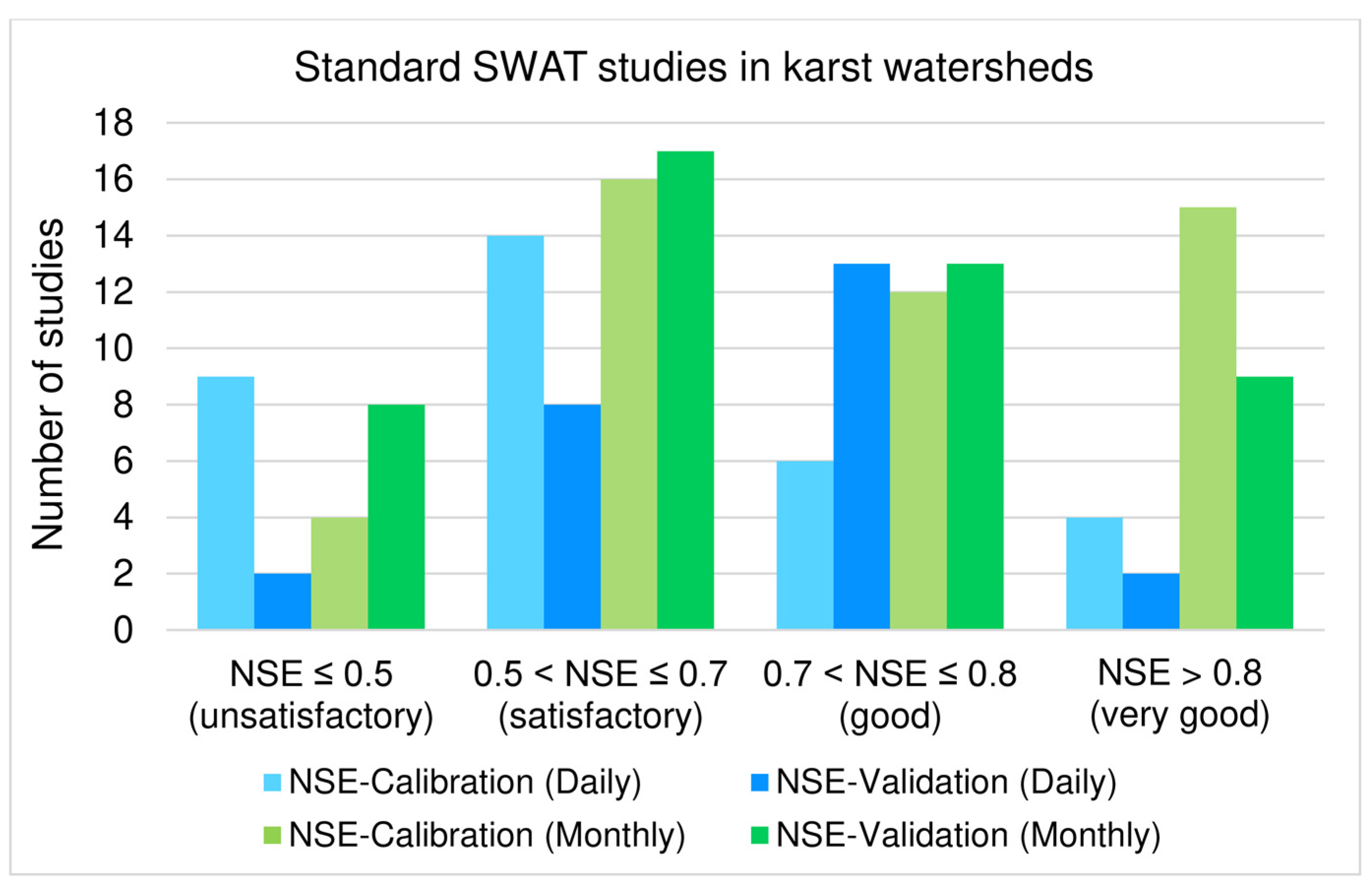
More than 70% of the studies that used NSE to assess the performance of SWAT hydrological models with daily time series calibration scored NSE values greater than 0.5, and over 90% reported NSE values greater than 0.5 for the daily time series validation. In comparison, more than 90% of the studies scored NSE values higher than 0.5 with monthly calibrated models, while upwards of 80% reported NSE values higher than 0.5 with monthly validation (Figure 2). These results indicate a satisfactory performance, with numerous applications meeting the criteria of a “good” flow simulation, as proposed by Moriasi et al. [102].

However, some applications conducted in complex karst watersheds scored poor NSE statistics. The studies conducted by Spruill et al. [104] and Coffey et al. [105] in the small experimental watershed of Kentucky revealed that SWAT failed to accurately reproduce peak and low flows. The observed and simulated daily hydrographs were asynchronous, with SWAT often underestimating the peak discharge rates and generating recessions that are faster than the observed data curves. The monthly runoff volumes at the watershed outlet were also underpredicted, which was attributed to the lack of explicit representation of karst geology in SWAT. A similar finding was reached by Benham et al. [106] who concluded that SWAT inability to reproduce the flows sustained by karst features reduced the prediction efficiency of streamflow in their study watershed. At a larger scale, the studies undertaken in the Scandinavian and Iberian peninsulas of 10⁶ km² and 556,000 km² [128], respectively, and in the Danube River basin of 800,000 km² [131] revealed that the performance of SWAT was lower in karst dominated regions in comparison to non-karst areas, due to the model misrepresentation of baseflow in karst streams. Martinez-Salvador and Conesa-Garcia [133] also emphasized on the need to improve the representation of extreme hydrological events (e.g., low flow and peak flow periods) in SWAT.

Furthermore, several studies underlined the need to account for external and interbasin groundwater flows to improve the discharge simulation in SWAT [104,121,124,127,134,137,141]. The hydrological simulations performed by Spruill et al. [104] confirmed the dye tracing results from sinkholes surrounding the study site that an area larger than the watershed topographic boundaries contributes to streamflow. Amatya et al. [107] underlined the need to couple SWAT with a subsurface hydrology model to accurately characterize the dynamics of the karst groundwater flow contribution to the surface drainage network. Gamvroudis et al. [127] estimated that around 33% of the water balance was lost via deep groundwater flow to areas outside their study watershed due to karst formations, while Palazón and Navas [124] simulated the discharge losses by underground flow through swallow holes in the upper part of the study basin. On the other hand, Jakada and Chen [141] confirmed the absence of runoff losses by subterranean flow diversion from their study watershed prior to conducting a hydrological simulation in SWAT. Their finding was based on the results of tracer tests conducted through the sinkholes in the watershed and monitoring of the springs within and outside the basin.

In more complex applications, Salerno and Tartari [121] coupled wavelet analysis with hydrological modeling in SWAT to identify the streamflow components in a non-conservative karst subbasin. After excluding the possibility of an incorrect assessment of the precipitation data, streamflow measurements, and evapotranspiration estimates, a series of continuous wavelet transform, cross wavelet transform, wavelet coherence, and phase difference analyses were applied to precipitation, groundwater levels, observed streamflow, and the time series constructed by the difference between the observed daily discharge and the streamflow simulated by a calibrated SWAT model of the study site. Based on the ensemble of correlations, it was established that the external water contribution to the river discharge was primarily due to groundwater seepage from a hydrogeological catchment that is larger than the surface watershed. The daily time series of the external water contribution was generated by multiplying the SWAT-simulated groundwater inflow by a yearly coefficient. This coefficient was adjusted to match the external contribution time series with the groundwater fluctuations simulated by SWAT and have the annual simulated flows equal to the observed flows. The additional water component improved the prediction efficiency of daily streamflow at the watershed outlet, with NSE increasing from 0.61–0.56 in the calibration and validation periods to 0.66–0.62, and R² increasing from 0.71–0.69 to 0.74–0.72. The mean absolute error of streamflow underestimation was also reduced from 47 to 33%.

Jian et al. [137] simulated discharge in a non-conservative karst watershed with an initial average discrepancy of 47% between the observed and measured water balances. After ruling out the possibility of invalid precipitation, evapotranspiration, and discharge measurements, the external contribution of the underground flow to streamflow was added as a point source discharge in SWAT, adopting the mean value of the difference in the annual water budget. The hydrological calibration and validation were carried out in a two-stage process. In the first step, the SWAT model and external flow value were calibrated using discharge data, while surface runoff, baseflow, and evapotranspiration were calibrated in the next step using available observational data. As a result, the baseflow component (excluding the external flow contribution) was calibrated in SWAT, and the inclusion of IGF reduced the underestimation bias of streamflow from nearly 50% to less than 3% at the monthly scale and 15% at the daily scale. NSE and R² values greater than 0.5 and 0.65, respectively, were also reached both in the calibration and validation periods.

More recently, Senent-Aparicio et al. [134] applied SWAT with the atmospheric Chloride Mass Balance (CMB) method to simulate streamflow of the Castril River basin (Spain). The study site is steep karst watershed fed by IGF from adjacent aquifers under steady conditions (i.e., no groundwater abstraction, evapotranspiration from shallow aquifers, or underflow to deep aquifers). The net aquifer discharge was equated to the baseflow component of streamflow, and the CMB approach was used to estimate the fraction of net aquifer recharge from the upstream areas as a proxy for the IGF contributing to additional baseflow. The corrected baseflow time series with IGF improved the SWAT model performance, reducing the underestimation bias of the streamflow simulations to less than 20% in both calibration and validation.

4.2. Applications of Modified SWAT in Karst Watersheds

4.2.1. Conceptual Linear One-Reservoir Model

This subsection describes the SWAT models with modified recharge functions and a linear one-reservoir groundwater module to simulate karst flows. These models include: the modified SWAT by [152], SWAT-B&B [153], SWAT-karst [154], KarstSWAT [155], and the modified SWAT by [156]. The latter four models can also represent karst watersheds dominated by flow through sinkholes.

Referring to Table 2, the first application of a modified SWAT code in a karst watershed was performed by Afinowicz et al. [152] to evaluate the impacts of woody plants management scenarios on the rangeland water cycle of the North Fork of the Upper Guadalupe River, Texas (USA). The watershed has an area of 360 km² and is covered by thin soils that overlie fractured limestone formations.

The return flow (baseflow) function of the groundwater module of SWAT (v2000) was modified to simulate rapid infiltration in karst areas into the deep aquifer. Therefore, the deep aquifer recharge component was deducted from the baseflow component of streamflow to allow a fraction of infiltrated water to bypass the shallow aquifer and enter the deep aquifer instead of flowing into the channel as baseflow, as shown in Equation (A1) of Appendix B.

The hydrological model was adjusted using daily streamflow data at the watershed outlet, with a 5-year warm-up period, a 5-year calibration period, and a 7-year validation period. The model scored monthly NSE values of 0.29 and 0.5 for the calibration and validation periods, respectively. It performed less efficiently at the daily scale, with NSE values of 0.4 and 0.09. It also failed to accurately reproduce all discharge trends at the daily scale, particularly high peak flows. The results of the hydrograph simulations were attributed to the nature of the surface runoff in the watershed, which is characterized by sustained low baseflow and very high flow that brings the soil water capacity to saturation.

Baffaut and Benson [153] modified the groundwater recharge equation of SWAT (v2005) to model fast infiltration from sinkholes and losing streams to the aquifer and groundwater flow contribution to surface water. The improved SWAT, known as SWAT-B&B/Adapted SWAT model, was applied to the 3600 km² James River basin in southwest Missouri (USA), characterized by losing streams, sinkholes, and springs.

In SWAT-B&B, recharge into the aquifer was partitioned to two components: (1) the infiltration from the soil bottom, representing slow flow to the porous matrix, and (2) the recharge from sinkholes and losing streams, representing fast flow to the conduits. Sinkholes in the study basin were modeled as ponds with a small drainage area and high hydraulic conductivity, while losing streams were represented by tributary channels with high streambed hydraulic conductivity. Thus, the soil and karst infiltration components were simulated using two recharge functions, each with a specific groundwater delay coefficient (see Equations (A2) and (A3) of Appendix C). Return flow was then modeled with the standard SWAT function, based on the groundwater flow of the previous day and the total aquifer recharge of that day (see Equation (A4) of Appendix C).

The hydrological model was calibrated for 8 years of daily streamflow records at 5 gauging stations and validated for 7 years. Streamflow biases were all less than 25%, ranging between 4% to 20% during the calibration period and −2% to −21% during validation. The percent of bias in surface runoff simulation were all around 10%, indicating a better representation of the baseflow component to streamflow. Moreover, NSE values of around 0.5 were reached for the calibration and validation periods in the main stem of the stream and at the outlet, but lower values close to 0.3 were obtained in the upstream small tributaries. Although a significant improvement in the NSE values could not be spotted by comparing both the standard and modified SWAT models, SWAT-B&B sustained more flows during the dry periods in comparison to SWAT.

The model was then used to estimate in-stream phosphorus loads and concentrations, and fecal coliform concentrations. Poor water quality simulation results were obtained in almost all observational river reaches of the basin, both in calibration and validation periods.

Yactayo [154] further modified the SWAT-B&B code to simulate fast aquifer recharge through sinkholes at the HRU scale by introducing a new parameter called sink to the HRU groundwater input file. This sinkhole partitioning coefficient represented the fraction of the runoff drained by a sinkhole to the unconfined aquifer. With this approach, a fraction of the surface runoff and lateral flow in the karst HRU was no longer included in the calculation of total streamflow in the main channel but allocated to the daily seepage from sinking streams and sinkholes. The transmissions losses from the surface runoff entering the sinkholes were also not simulated. Thus, the unconfined aquifer recharge in non-karst regions was calculated using Equation (A5) of Appendix D, whereas aquifer recharge in karst regions was computed using Equation (A6) of Appendix D.

The modified model known as SWAT-karst was applied in the 890.2 km² Opequon Creek watershed, located in the Potomac and Shenandoah River basin in Virginia. For SWAT-karst, a new land-use category was added to the land-use map so that sinkholes may be represented by HRUs, based on the area of the sinkhole regions and the land use where the sinkholes are located. Similar to SWAT-B&B, sinking streams were represented by tributary channels with high hydraulic conductivities.

SWAT-karst, SWAT-B&B and SWAT were run at the daily time step for a period of 11 years and compared in terms of their performance efficiency in simulating streamflow and other water balance components without any model calibration. All three models overestimated streamflow, and the values of the PBIAS, NSE, and RSR were unsatisfactory at all subbasin outlets and streamflow gages where discharge values were compared. Nonetheless, both SWAT-B&B and SWAT-karst performed better than SWAT in simulating karst discharge, and SWAT-karst had a more significant impact on the distribution of the water balance components, by simulating less runoff and more baseflow in karst regions with sinkholes. The authors noted that aquifer recharge diverted by sinkholes to regions outside the watershed could be a reason behind SWAT-karst overestimating discharge and failing to meet the acceptable performance criteria. However, they maintained that parameter sink values could be modified to control the depth of water that recharges the unconfined and confined aquifers (water lost from the watershed, see Equation (A7) of Appendix D). Yactayo [154] also modeled the nitrate loading that recharges the aquifers through the sinkhole as a function of: (1) the volume of surface runoff and lateral flow lost to sinkholes in karst regions, and (2) the nitrate aquifer recharge loading from the soil water percolation. Similar to the flow simulation results, the values of the in-stream nitrate concentrations calculated from aquifer recharge and nitrate in baseflow were unsatisfactory.

On the other hand, Palanisamy and Workman [155] incorporated an orifice flow transfer function and a successive summation routing algorithm (SSRA) into SWAT in order to simulate groundwater flow from sinkholes located in the streambed to a spring. The modified SWAT code, called KarstSWAT, was applied to the Cane Run watershed of 115.6 km² in Kentucky (USA), where numerous sinkholes found along the river streambed divert surface runoff through an underground conduit to the main watershed spring. The karst aquifers to which sinkholes drain the river flow largely overlap the Cane Run surface watershed, and runoff routing into the sinkholes depends on the incoming streamflow volume, the sinkhole size, and the capacity of the underground conduit.

To represent this unique hydrological setting, sinkholes were conceptualized as orifices and were modeled as outlets of the karst subbasins during watershed delineation in SWAT. The discharge capacity of the sinkholes was simulated using a head-discharge relationship (see Equation (A8) of Appendix E) as a function of a diameter range that corresponds to the size of the sinkholes. The discharge from the sinkholes and infiltration from the soil profile bottom were then added to the deep aquifer reservoir in SWAT, aggregated at HRU level, and transferred to the spring outlet using the SSRA algorithm with a maximum travel time of one day. The number of the subbasin in which the sinkholes are located and the diameter of the sinkholes were specified in an input file called sink.dat, while groundwater basins that drain the aquifer water to the spring were defined in a file called gw_flow.dat.

KarstSWAT was calibrated for 3 years using daily streamflow measurements at the Cane Run River, and validated for another 3 years using runoff data at the Cane Run River and spring outlet. Compared to the original SWAT model, KarstSWAT showed a better representation of the hydrological cycle in the karst watershed. The average annual surface runoff and recharge to shallow aquifer decreased by 65% and 91%, respectively, while deep aquifer recharge increased many folds as water was partially diverted through the sinkholes rather than the soil. The cumulative observed and simulated streamflow plots, with and without sinkholes, also demonstrated that KarstSWAT reduced channel flow during low flow and high flow periods. The modified model performance was further assessed against the original SWAT model under a multitude of runoff events during which at least 10 mm of peak rainfall was observed. Results showed that KarstSWAT improved the prediction of the peak flows and baseflow, with average the NSE and R² values increasing from 0.23 to 0.77 and 0.78 to 0.87, respectively. Moreover, the discrepancy between the observed and simulated spring flow was attributed to the capacity of the orifices to transfer flow, whereby the overestimation of streamflow by KarstSWAT resulted in the underestimation of spring discharge and vice versa. Nonetheless, discharge at the watershed spring was continuously simulated, showing a good agreement with the observed spring hydrographs at different time periods.

Zhou et al. [156] also modified SWAT (v2012) to simulate fast infiltration through karst sinkholes in the upper course of the South Panjiang River, Southwest China. The basin extends over an area of 2762 km² that is mainly covered by limestone and under the influence of a subtropical humid monsoon climate. Due to the karst effect, sinkholes have formed across the watershed subbasins as opposed to only in the streambed (the case of the study the Cane Run watershed [155]).

The authors used the pond module of SWAT to represent the sinkhole processes. While infiltration from the bottom of the soil profile in both karst and non-karst areas is modeled using the same delay time variable in the original SWAT, the recharge function was modified to simulate the rapid recharge of groundwater aquifer in sinkholes. Water leaving the ponds to the aquifer was separated from percolation with a delay time variable specific to pond leakage and set to 1/50 of its original value. Hence, recharge was divided into two components: leakage recharge of the soil profile and rapid recharge of the karst sinkholes (Equation (A9) in Appendix F). The pond module was added at the subbasin scale, and sinkholes were represented by one pond in each subbasin whereby a fraction of the subbasin area drains the surface flow into the pond. A high hydraulic conductivity value was set at the bottom of the ponds in order to maximize infiltration and groundwater recharge.

The SWAT model was adjusted using monthly streamflow data, with 2 years of warm-up, calibration, and validation each. The modified SWAT model improved the streamflow simulations: the values of the NSE and R² indicators increased from 0.35–0.66 (calibration-validation) and 0.7–0.76, respectively, in the original SWAT to 0.61–0.79 and 0.74–0.83 in the modified SWAT, with a higher prediction accuracy of the peak flow and baseflow at the daily time interval. The use of the pond module, with large hydraulic conductivity values and short recharge durations, also reduced the surface runoff and lateral flow in the subbasins with sinkholes and increased baseflow depth by rapidly diverting the surface water to the shallow aquifer.

4.2.2. Conceptual Linear Two-Reservoir Model

This subsection describes the modified SWAT models with a linear two-reservoir groundwater module to simulate flows of the matrix and conduits components in a karst system. These models are Karst-SWAT [157], KSWAT [165], and SWAT_IFG [166].

Nikolaidis et al. [157] interfaced SWAT with a spreadsheet version of the linear two-reservoir model proposed by Kourgialas et al. [178] to simulate discharge and nitrate transport in the Koiliaris River basin (132 km²) in Crete, Greece, under climate change. The modified SWAT model, known as Karst-SWAT, comprises an upper reservoir representative of the fast flow in the conduits and a lower reservoir for the slow flow in the matrix and narrow fractures. The model uses two proportionality coefficients to partition karst recharge between the two compartments and models another flow fraction from the upper to the lower reservoir. The sum of outflows from the matrix and conduit reservoirs forms the total discharge of the karstic area (see Equations (A10) to (A14) in Appendix G).

In the case of the Koiliaris River basin, the recharge area of the springs contributing to the total watershed flow extends at least 50 km² beyond its boundaries. Nikolaidis et al. [157] first used SWAT to model the surface hydrological processes (precipitation, evapotranspiration, infiltration, runoff) and route the percolated water to the deep groundwater aquifer. The extent of karst areas contributing to the emergence of springs from outside the watershed boundaries was established based on the geologic knowledge of the study site and a mass balance modeling approach. Then, the SWAT-simulated deep groundwater flow in karst areas was assigned to the karstic reservoir model in order to estimate the spring flow contribution to discharge. After calibration of the reservoir model parameters, the resultant karst flow time series were input to SWAT as a point source to simulate the overall watershed runoff.

The parameters of the karst flow reservoir and SWAT models were adjusted using high frequency flow measurements at the watershed outlet, surface runoff measurements at a major tributary of the river, and long-term monthly spring flow records. The overall model prediction efficiency of discharge was satisfactory. At the monthly time step, NSE values of 0.77–0.61, PBIAS of −22.1%; −11.8%, and RSR of 0.62–0.63 were reached during calibration and validation, respectively, whereas NSE of 0.62–0.43, PBIAS of (−22.3%; −11.6%), and RSR of 0.48–0.75 were achieved for the daily runoff simulations.

From the water quality perspective, Nikolaidis et al. [157] incorporated a nitrate mass balance model to the upper and lower reservoirs of the karst flow model, assuming that nitrate is conservative in karst. A karst factor was added to the nitrate mass balance equation of the lower reservoir to account for the extra dilution of the incoming nitrate loads by the permanent karst flow volume below the spring level. After calculating the nitrogen inputs in the watershed and the extended karst recharge area based on the local land-use practices, the hydrological and water quality modeling parameters were adjusted using nitrates grab sample data at a river tributary and groundwater wells, coupled with high frequency nitrate data, grab samples at the watershed outlet, and flow measurements. The simulated nitrate concentrations were adequate compared to the nitrate grab sample measurements.

The impact of climate change on the water budget of the Koiliaris River basin was also predicted up to the year 2050, using three climate change scenarios for a combination of general and regional circulation climate models. The results of the climatic projections suggested that precipitation, evapotranspiration, and runoff could decrease by 17%, 8%, and 22%, respectively, for the time horizon 2030–2050 compared to 2010–2029.

Nerantzaki et al. [158] later adopted the Karst-SWAT flow model by Nikolaidis et al. [157] to first simulate the hydrology and suspended sediment transport in the Koiliaris River basin then predict the impacts of climate change on discharge, soil erosion, and sediment transport. The concentration of suspended sediments in the karstic watershed was calculated using the same mass balance equations and deep karst factor adopted by Nikolaidis et al. [157] for nitrates. Four additional years of simulation were added to the validation period of the model previously calibrated by Nikolaidis et al. [157]. Next, climate change scenarios were run up the year 2090 after adjusting the most sensitive flow and water quality parameters. The results of the discharge simulations were adequate, with daily NSE, PBIAS, and RSR of 0.8, 25.3%, and 0.45, respectively, and monthly NSE, PBIAS, and RSR of 0.83, 23.4%, and 0.41, respectively. The suspended sediments calibration results were less adequate, with daily NSE of 0.7, PBIAS of 57%, and RSR of 0.55, suggesting an overestimation bias.

The results of the climate change scenarios showed that surface runoff and spring flow could decrease by nearly 70 to 77% between the time periods of 2010–2049 and 2050–2090. The erosion rate of the watershed main subbasin and surface sediments export were also expected to drop by 48% and 55%, respectively, whereas sediments emerging from the springs were not substantially affected by climate change.

Following an analysis of climate change impacts in the Crete Island using Karst-SWAT, Demetropoulou et al. [160] proposed a program of measures to improve water governance in the 525 km² Geropotamos basin located in central-southern part of the island. Nerantzaki et al. [161] also used Karst-SWAT to forecast the hydrological response of the Crete region under climate change scenarios up to the year 2098, considering different irrigation sources in SWAT. Moreover, Tapoglou et al. [159] applied Karst-SWAT to predict the impact of climate change on the hydrological cycle and the frequency of extreme hydrological and meteorological events in Crete. Nerantzaki et al. [163] further expanded the research work conducted in the Koiliaris River basin with Karst-SWAT by assessing: (1) the uncertainty of the watershed runoff and karstic flow simulations due to the parameter uncertainty in SWAT and Karst-SWAT, and (2) the impact of internal variability (or stochastic uncertainty) of the meteorological input data on the flow simulations for the reference period and under the climate change scenarios. The uncertainty of the flow models was estimated by combining the Sequential Uncertainty Fitting Version 2 (SUFI-2) in the SWAT Calibration and Uncertainty Program (SWAT-CUP) interface and the @RISK by PALISADE software, while the effect of input internal variability on the flow output was evaluate using Monte Carlo simulations.

Within the framework of studying the hydrological and geochemical processes in the Koiliaris European Critical Zone Observatory, Lilli et al. [164] used Karst-SWAT to simulate the hydrological budget of the Koiliaris River basin and gain insight on the hydrological pathways and response of the karst during extreme events. Additionally, Karst-SWAT was applied to simulate surface flow and spring flow in the Koiliaris River basin, which were required to determine the design flows and flood frequency within the framework of developing nature-based solutions for the riparian forest restoration and flood protection project at the Koiliaris Critical Zone Observatory [162].

Next, Malagò et al. [165] developed a two-reservoir modeling approach by linking SWAT-B&B [153] and Karst-SWAT [157]. The resultant hybrid model, called KSWAT, was used in conjunction with SWAT to simulate the water balance, spring flow, and total discharge in the Island of Crete in Greece. The study area extends over 8336 km² of which 2730 km² is karst.

A SWAT model of the Crete Island was set up and the modified model KSWAT was applied only in the karst subbasins of the region. The daily aquifer recharge from the karst subbasins was simulated using SWAT-B&B. The area of the subbasins contributing to the recharge of a particular spring or group of springs was identified based on the local geological maps and dominant karst soils. Recharge from the soil profile bottom, stream losses, and seepage from other water bodies to the deep aquifer were maximized by: (1) setting the deep aquifer percolation fraction and minimum groundwater delay to 1, (2) adjusting the groundwater coefficient of capillary rise to 0.1 to prevent the upward movement of water to the unsaturated zone, and (3) minimizing the return flow from the shallow and deep aquifers in SWAT. The deep aquifer recharge time series generated by SWAT-B&B were then input to Karst-SWAT in order to simulate and calibrate the discharge of the springs. The parameters of the Karst-SWAT model were adjusted based on daily spring discharge data from 47 gauging stations in Crete.

The hydrologic model in SWAT was adjusted using a step-wise calibration with monthly streamflow data at 15 stream gauging stations. Snow, surface runoff, lateral flow, and baseflow parameters were first calibrated separately in order to adjust the timing of the runoff signal and the discharge values (peak flow and baseflow). Then, the model was recalibrated based on the streamflow-related parameters combined with the adjusted variables of the other water budget components. The final near optimal parameter set of the calibrated subbasins was transferred to the ungauged subbasins using the hydrological similarity approach with the Partial Least Squares Regression, in order to identify similar subbasins based on the correlation between the watershed and discharge characteristics.

Subsequently, the calibrated spring discharge time series from Karst-SWAT were added to the Crete SWAT model as point sources in order to predict the total monthly runoff across the island, and a final calibration was performed to adjust discharge. The results of the performance indicators showed that only 40% of the calibrated gauging stations scored NSE values greater than 0.5, while 50% had R² values higher than 0.5 and 64% reached PBIAS lower than 25%.

Moreover, Nguyen et al. [166] added a two-reservoir karstic flow model to the original groundwater module of SWAT. The improved SWAT code, termed SWAT_IFG, consists of two conceptual groundwater models compiled in a single executable file: (1) the standard SWAT one-reservoir model applied to non-karst terrains, and (2) the modified two-reservoir model used in karst areas. The two-reservoir groundwater model of SWAT_IGF represents a variant of the Karst-flow model by Nikolaidis et al. [157]. In SWAT_IGF, the matrix reservoir receives diffuse recharge as a linear function of daily infiltration from the soil bottom, considering the time delay of flow in the unsaturated zone (Equations (A15) and (A16) of Appendix H). The conduit reservoir receives another fraction of the soil water seepage as concentrated recharge with infiltration losses from sinking streams. It is also fed by diffuse discharge from the matrix reservoir, which represents the flow exchange mechanism between the two karst domains (Equations (A18) and (A19) in Appendix H). Groundwater outflow from the matrix storage reservoir to the conduit is modeled using a linear storage-discharge equation with a matrix recession coefficient (Equation (A17) in Appendix H). Outflow from the conduit reservoir to the spring is also modeled via a linear storage-discharge relationship adjusted for the total recharge volume to the conduits and a conduit recession coefficient (Equation (A20) in Appendix H). The total discharge of the basin where the spring is located is then simulated as the sum of the direct runoff (surface runoff and lateral flow) and the outflow from the conduit reservoir to the spring (Equation (A21) in Appendix H). Consequently, SWAT_IGF can simulate surface runoff and subsurface flow in non-karst and karst areas. It can also account for the dual recharge and storage functions of the matrix and conduits. and model spring discharge in regions where the karst aquifer boundaries do not coincide with the surface subbasin areas.

SWAT_IGF was applied to simulate discharge in the drainage basin of the karst dominated southern Harz rim and non-karst southwest Harz Mountains in Northern Germany. The watershed covers an area of 384 km² and has one river outlet and a main spring outlet (the Rhume spring). The spring is mainly fed by allogenic recharge and river transmission losses from upstream subbasins via a connected network of losing streams in the area, with only 4% of the spring discharge originating from autogenic recharge and nearly 96% from IGF.

When applying SWAT_IGF, an aquifer classification map with information about the aquifer types and spring recharge area in the study site was incorporated into the model to delineate karst and non-karst HRUs. Subsequently, the suitable conceptual reservoir model could be assigned (the two-reservoir model for the karst HRUs and the one-reservoir model for the non-karst HRUs), and recharge from the extended karst area could be routed to the spring outlet.

SWAT_IGF was run for 14 years at the daily time step, with 3 years of warm-up, 6 years of calibration, and 5 years of validation. The model parameters were fitted based on multi-site daily streamflow data and satellite-derived actual evapotranspiration records (the Moderate Resolution Imaging Spectroradiometer MOD16 ETa). A multi-criteria NSE objective function was used to assess the overall performance of the model simulation, with equal weights allocated to the multi-gauge streamflow observations and evapotranspiration data. Results showed that the use of MOD16 ETa data in the calibration did not affect the model performance. The flow simulation at the spring outlet improved with multi-gauge calibration, as the NSE values varied from 0.75–0.48 (calibration-validation) with the single gauge calibration to 0.69–0.62 under the multi-site calibration. The model performance for all remaining streamflow gauging stations also improved with multi-site calibration, and NSE values of 0.54–0.91 and 0.6–0.91 were reached for the calibration and validation periods, respectively. Additionally, the model prediction uncertainty was reduced. The PBIAS values calculated at the different gages fell below 10%, while KGE values ranged between 0.68 and 0.91. Yet, the observed and simulated streamflow hydrographs showed that SWAT_IGF underestimated the high and low flows, which is a property inherited from the original SWAT model. Nonetheless, the model successfully simulated IGF and transmission losses from the rivers contributing to the spring discharge.

4.2.3. Conceptual Linear Three-Reservoir Model

This subsection describes the modified SWAT models with a linear three-reservoir groundwater module to simulate flows of the main karst aquifer components (i.e., epikarst, matrix and conduits). These models include the modified SWAT by [167,168].

Wang et al. [167] coupled SWAT (v2012) with a linear three-reservoir model. The modified model consists of: (1) an upper reservoir that reproduces the regulation and storage function of the epikarst and is recharged by percolation from the soil bottom, (2) a middle reservoir that represents the conduits system fed by infiltration from the epikarst, depressions, and avens, and (3) a lower reservoir corresponding to the matrix system recharged by the epikarst and conduit reservoirs. Daily infiltration to the upper reservoir is simulated as a function of the saturation moisture content in the epikarst system, its water-holding content, and saturated hydraulic conductivity (Equations (A22) and (A23) of Appendix I). To simulate the intercompartment fluxes, a proportionality coefficient (${\alpha }_1:$ 0.5–1) is introduced to separate the recharge from the epikarst reservoir between the quick flow and slow flow reservoirs, based on the degree of karstification of the watershed. Another coefficient (${\alpha }_2:$ 0.1–0.5) is used to split the discharge from the conduit reservoir between the slow flow reservoir and the basin outlet (Equations (A24) and (A25) of Appendix I). The outflows from the conduit and matrix reservoirs are modeled using the standard attenuation functions of SWAT (See Equations (A26) and (A27) of Appendix I). Finally, the total karst flow is calculated as the sum of the discharge components of the matrix and conduit reservoirs (Equation (A28) of Appendix I), which is then added to the surface runoff to simulate the total discharge at the watershed outlet.

The original and modified SWAT models were applied to predict daily runoff for a fully karstified watershed of 26.76 km² located in Hunan Province, China, with a calibration period of 180 days and a validation period of 100 days. The study area is primarily covered by Devonian and Carboniferous limestone and exhibits karst depressions, caves, and underground rivers. The SWAT three-reservoir model yielded a streamflow simulation that was significantly better than that obtained by the standard SWAT model in both calibration and validation, with NSE values increasing from 0.57–0.63 to 0.81–0.83 and R² values increasing from 0.58–0.62 to 0.82–0.84.

Geng et al. [168] later modified the SWAT model proposed by Wang et al. [167] in order to improve the simulation of rapid recharge to the epikarst reservoir through direct water percolation from the soil bottom without attenuation. The modelers also added a discharge component from the epikarst reservoir to the river channels. Three coefficients of proportionality were thus introduced to the three-reservoir groundwater model in order to separate the flow from the epikarst reservoir between a surface runoff component and two recharge components to the matrix and conduit reservoirs (See Equations (A29) to (A31) of Appendix J). Rapid infiltration through sinkholes, ponors, and fractures was also replaced by pond leakage with concentrated (fast) recharge similar to the computational method proposed by Baffaut and Benson [153]. The remaining intercompartment fluxes were modeled similarly to the model by Wang et al. [167].

The modified SWAT model was applied to simulate the hydrological cycle processes in the Daotian River basin, including the contribution of the streamflow and baseflow components to the runoff at the watershed outlet. The study site is situated in the Guizhou Province, China, and has a temperate monsoon climate. It covers a total area of 99.21 km² of which ~53% is dolomite, ∼38% limestones, and ∼9% clastic rocks. The karst landscape is characterized by karst depressions, sinkholes, and well-connected networks of conduits of high hydraulic conductivity, particularly in the limestone area. Due to karst effects, the watershed recharge boundaries extend by 24.75 km² beyond its surface drainage area, and the additional water is discharged into the watershed through underground conduits. The areas outside the topographic drainage divides and the flow paths of the karst subterranean rivers that exist in the watershed were determined by conducting a karst survey and an artificial tracer test prior to hydrological modeling. After determining the flow paths of the subterranean river based on the spatial distribution of the subterranean river inlet, ponors, and sinkholes, the DEM data were modified to convert the subterranean river into a surface river. By adopting this approach, the actual catchment boundaries of the watershed were correctly identified by SWAT for the subbasins delineation.

The modified SWAT model was calibrated using daily streamflow measurements at the watershed outlet for 6 years (1993–1998). Two validation periods were considered under various annual precipitation patterns: the first from 1999 to 2002 (normal, dry, and wet years) and the second from 2003 to 2006 (normal and dry years). The performance of the modified SWAT model was compared to that of a previous model run in SWAT at monthly time scale. Both models had satisfactory simulations of monthly discharge. Yet, the modified SWAT model had a better prediction efficiency than the original SWAT, scoring NSE values of 0.87–0.83/0.85, R² of 0.88–0.84/0.86, and PBIAS of 2.5%–(−1.9%/−15%) for the calibration and two validation periods, respectively. The three-reservoir model also improved the simulation of the karst water cycle by increasing the groundwater recharge and return flow components. As a result, the NSE for the baseflow simulation of the modified SWAT model was 0.09 higher than that of the original SWAT model, which underestimated flows below 0.7 m³.s⁻¹ in the dry periods and overestimated runoff during wet periods.

4.2.4. Conceptual Non-Linear One-Reservoir Model

To the best of our knowledge, a non-linear groundwater reservoir has been previously implemented few times in SWAT to: (1) model groundwater flow in a karstic aquifer [169], (2) estimate baseflow in rivers dominated by snow and glacier melt [179], and (3) improve the prediction of streamflow in watersheds with complex groundwater processes under heavy irrigation pumping [180].

Wang and Brubaker [169] replaced the linear reservoir model in SWAT with a single non-linear reservoir based on the algorithm of Wittenberg [181] (see Equations (A32) and (A33) of Appendix K), providing a modified SWAT version called ISWAT. The ISWAT model was tested in the Shenandoah River watershed of the Potomac River basin (USA), which drains a large karstic area of 7607 km². It was calibrated using 13 years of daily discharge records across 14 gauging stations, with 2 years of warm-up, and validated for 4 years. To account for the spatial variability of the geology and soils in the watershed during calibration, the parameters of the non-linear reservoir (i.e., groundwater recession coefficients and exponents) were grouped by soil type.

The ISWAT model performance was assessed against that of the linear SWAT model by comparing the simulated and observed streamflow hydrographs at the different gauging stations, and the recession curves in the low flow periods with the baseflow taken as the lowest 30% of daily discharge. The non-linear ISWAT model reproduced low flow discharge and recession curves better than SWAT, but simulated peak flows with a comparable accuracy to SWAT. The NSE (modified) and R² indices improved with the use of the non-linear model at the level of eight and ten observational river reaches, respectively, with values of 0.5 and 0.6. The non-linear model also lowered the overall relative bias of the simulations by 3%, with the majority of the observational river reaches scoring a bias less or equal to 10%.

4.2.5. Modified Crack Flow with Conceptual Linear One-Reservoir Model

This subsection summarizes the application of the modified SWAT models by [36], which were adapted to simulate fast recharge in karstified watersheds based on the crack flow approach in SWAT.

Eini et al. [36] modified SWAT (v2012) to increase groundwater recharge in karst areas by: (1) adjusting the groundwater recharge function in SWAT to increase infiltration in karst HRUs (the SWAT-ML model), and (2) expanding the crack flow module in SWAT to retain the formation of cracks independently of soil moisture conditions (the SWAT-CF model). These modifications were based on the premise that preferential flow through the soil sinks and cracks can be representative of rapid recharge in karst landforms.

Both SWAT-ML and SWAT-CF were applied in the Maharlu Lake, a large watershed of 4270 km² in Southwest Iran, of which 37% is covered by extensive karst areas (limestone and dolomite). Several karst-fissured aquifers are well developed in these areas due to lithology, climate, and tectonic activity.

In SWAT-ML, infiltration from non-karst areas was calculated using the standard SWAT recharge equation (Equation (A34) of Appendix L), while fast infiltration from karst areas was modeled by dividing the delay variable in the original groundwater recharge equation by a new non-dimensional calibration parameter (X) (Equation (A35) of Appendix L). This parameter can be increased depending on the volume and numbers of cracks in a karst HRU.

In SWAT-CF, the standard SWAT function that calculates crack volume during the crack flow process was modified by adding a new parameter of the crack volume based on new moisture conditions (Equation (A36) of Appendix L) to achieve a year-round crack formation in the soil matrix. As a result, SWAT-CF can simulate crack flow in karst HRUs both in dry and wet soil conditions during surface flow events, as opposed to standard SWAT, which only models crack volume on drier days as a function of crop capacity and soil moisture.

The hydrological models developed with SWAT, SWAT-ML, and SWAT-CF were run using streamflow data recorded at 3 gauging stations, with 3 years of warm-up, 26 years of calibration, and 4 years of validation. Both modified SWAT models outperformed SWAT in simulating monthly streamflow at different stations, with SWAT-ML having the best overall accuracy. The average NSE value increased from 0.64 with SWAT to 0.67 using SWAT-CF and 0.69 using SWAT-ML, while the average R² value varied from 0.70 to 0.69 and 0.72 under SWAT-CF and SWAT-ML, respectively. The modified models also increased the prediction accuracy of the baseflow and water budget components.

4.2.6. Variable Source Area Hydrology with Conceptual Linear One-Reservoir Model

Topo-SWAT (initially termed SWAT-VSA) is a modified version of SWAT that was applied to simulate flow, sediments yield, and nutrients loads in a watershed with variable source area (VSA) hydrology [170]. Compared to SWAT, Topo-SWAT incorporates a topographic wetness index (TI) that indicates the saturation potential of a landscape unit and the subsequent likelihood of runoff generation. Ten equal-area wetness classes ranging from 1 to 10 (1 being 10% of the watershed with the lowest runoff potential, and 10 being 10% of the watershed with the highest runoff potential) were used to overlay a wetness class layer with the soil map of the study site and generate a single GIS layer and associated lookup tables for the SWAT slope class and soil layers.

Topo-SWAT was tested in the Spring Creek watershed in northeastern USA. Spring Creek has a surface water watershed area of 370 km² but is defined by a groundwater recharge boundary of 450 km², which is characterized by saturation excess surface runoff from VSAs (e.g., perched and losing streams in the headwater regions of the watershed, low surface runoff in the forested uplands due to quick infiltration through shallow soils, overland flow generated at the base of hillslopes). Some of the adjustments made to the model parameters to accurately represent karst hydrology in the study watershed included reducing the initial curve number, restricting the groundwater delay factor to 1 day, setting the baseflow recession factor to 0.011 day based on observed daily streamflow records, and introducing the contribution of the springs that recharge outside Spring Creek but discharge inside the watershed as point sources.

Topo-SWAT outperformed SWAT in modeling daily streamflow for a 12-year simulation period, with NSE of 0.73–0.79, PBIAS of −2.8 to −3.7%, and R² of 0.71–0.77 in the calibration and validation periods. Moreover, Topo-SWAT successfully reproduced the VSA hydrology of the watershed using the wetness class distribution approach and predicted water quality adequately.

The calibrated Topo-SWAT model of the Spring Creek watershed was later used to simulate nutrient and sediment loadings under four dairy cropping scenarios of different land areas, feed production, and nutrient input strategies [171]. The model was also applied to evaluate the impacts of agricultural best management practices on nutrient water quality in the watershed [172]. Gunn et al. [173] further modified SWAT-VSA by integrating a daily dynamic time series of CO₂ into the model and implementing changes to the plant subroutines to additionally include flexible stomatal conductance and LAI parameters. The generated models, namely SWAT-VSA_CO2 and SWAT-VSA_CO2+Plant, were used to predict the impacts of climate change with increasing atmospheric CO₂ on the water balance of the Spring Creek watershed.

4.2.7. SWAT + Water Accounting Plus (WA+) Framework

Delavar et al. [174] coupled SWAT with the Water Accounting Plus (WA+) framework, providing a hybrid tool to analyze water resources and support macro and micro water planning in watersheds, based on past, current and future trends in water demand and supply. WA+ uses four sheets to assess water resources in a basin, including resource base, evapotranspiration, productivity, and withdrawal components. In order to populate these sheets with input data generated by hydrological simulation in SWAT, the SWAT source code was modified to: (1) simulate and report the daily groundwater level changes, and (2) model the interactions and exchanges between the aquifers located in different subbasins by overlaying the subbasin HRUs layer and aquifer boundaries during HRUs definition. The SWAT-WA+ tool was used to evaluate the trends in water supply and consumption in the Tashk-Bakhtegan karst watershed (27,520 km²) in Iran, where 60% of the irrigation demand is met by groundwater. Delavar et al. [175] remodified SWAT (v2012) and linked it with WA+, adding the crack flow module proposed by Eini et al. [36] with the other modifications previously implemented by Delavar et al. [174] to link SWAT and WA+. The model was applied to assess different conditions of water supply and demand under wet and dry periods in the karstified Karkheh River basin (42,267 km²) in Iran.

The customized SWAT-WA+ frameworks, namely SWAT-FARS for the Tashk-Bakhtegan basin and SWAT-Karkheh for Karkheh River basin, were calibrated for streamflow, groundwater levels, evapotranspiration, and crop yields using a multi-stage calibration process. Both models scored NSE and R² values higher than 0.5 for the streamflow and groundwater levels simulations in the calibration and validation periods. The outputs of the modified SWAT models were then used to run the WA+ framework. The results of the WA+ assessments revealed that the Tashk-Bakhtegan basin has suffered a decline in the volume of manageable water by more than 20% while irrigation demand increased by more than 50%, and that the volume of manageable water in the Karkheh River basin has dropped while groundwater abstraction increased by 17% due to climate change.

4.2.8. Overall Performance of Modified SWAT Models

Based on the reviewed literature, a total of 18 modified SWAT models have been developed and applied across 25 studies in watersheds characterized by karst geology (Table 2). Models that were run at daily and monthly time intervals reported a higher prediction efficiency of the flow at the monthly scale than the daily scale, both in calibration and validation periods [152,157,163,170]. Around 80% of the studies that used NSE to evaluate the hydrological model performance at the daily time step reported NSE values greater than 0.5 for the calibration and validation periods. In comparison, more than 80% of the studies that used the monthly time step scored NSE values higher than 0.5 for calibration, and more than 90% reported NSE values greater than 0.5 for validation (Figure 3).

Several applications showed that accounting for external flows from sinkholes and IGF, in conjunction with the implementation of reservoir models in SWAT, is needed to achieve an adequate representation of karstic flows [155,157,158,163,166,167,170,174]. Overall, coupling SWAT with karst flow models and adding external functions that reproduce karst features and processes to the SWAT source code have resulted in semi-distributed karstic flow models that simulated discharge with a comparable or better prediction efficiency than standard SWAT [36,155,156,167,168,169] while accounting for the dynamics of the different components in a karst system (when applicable).

However, poor daily and monthly performance statistics were still reported by Afinowicz et al. [152], Baffaut and Benson [153], and Malagò et al. [165] following the modification of the SWAT code. These results which suggest that modified approaches applied to the groundwater recharge and reservoir functions in SWAT may not always guarantee a successful simulation of the flow in complex karstic environments. For instance, Afinowiz et al. [152] indicated that additional modifications to the SWAT flow modules could be required to adequately simulate the large volumes of surface runoff and return flow during flood events as opposed to baseflow during low flow periods. Additionally, we could not identify published studies in which the modified SWAT models were applied across different watersheds, with the exception of the Karst-SWAT model [157] which has been used in the Koiliaris River Basin and the Island of Crete for a multitude of applications (i.e., hydrological and geochemical analyses, climate change impacts, management practices). Thus, one could infer that these models have not been widely tested in other karst basins or they only worked for watersheds with comparable geomorphological and hydrogeological characteristics to the basins in which they were initially applied. Consequently, the modified SWAT models listed in Table 2 can be further improved to have a better representation of karstic heterogeneity and non-linearity in their structure.

5. Recommendations and Perspectives for Future Research

5.1. Constraints of Modified SWAT Models in Representing Karst Flow Characteristics

Highlighting the constraints of the modified SWAT models (Table 2) would be the initial step to enhance their adaptability to other karst watersheds with complex surface water-groundwater hydrodynamics.

First, the Karst-SWAT [157] and KSWAT [165] two-reservoir models do not consider the function of the epikarst and do not explicitly include the diffuse and concentrated recharge components of infiltration from the karstic soils to the deep aquifer reservoir in SWAT. Both models use the exponential decay weighting function to simulate recharge and outflows of the matrix and conduit reservoirs. However, the non-linear models are generally more suitable than the linear ones in representing the hydraulic behavior of karst systems, particularly during low flow periods and flood events [182,183,184]. Moreover, the two models follow the watershed surface delineation in SWAT to determine the recharge area of the spring, which may not always coincide with the groundwater recharge boundaries. This requires a tedious assessment of the karst areas recharging the springs outside the watershed in tandem with the introduction of the spring flow time series contributing to the watershed discharge as point sources in SWAT to simulate IGF.

Some of the Karst-SWAT and KSWAT modeling constraints were improved in the two-reservoir SWAT_IGF model [166], which simulates the hydrological processes in non-karst and karst regions as well as IGF in a single executable file. Although SWAT_IGF considers the dual recharge and storage functions in karst systems, it uses the linear storage-discharge relationship to model the outflows of the matrix and conduit reservoirs, and does not account for the function of the epikarst either. In SWAT_IGF, the exchange flow rate between the matrix and conduits is simulated as a diffuse net unidirectional flow from the matrix to the conduit. Yet, flow can be transferred from the conduit to the matrix, and vice versa, based on the change in the water level gradient between the two mediums. Additionally, SWAT_IGF models the spring flow contribution to discharge in karst areas as a single outflow from the conduit reservoir, whereas both the matrix and conduits can contribute to the karst discharge with different flow regimes (slow matrix discharge during low flow periods and fast conduit discharge during heavy rainfall seasons).

Next, the three-reservoir models developed by Wang et al. [167] and Geng et al. [168] incorporate the epikarst, matrix, and conduit functions, and thus represent a complete underground karst system. Yet, their main constraint is that fluxes between the reservoirs are simulated using a linear storage–discharge relationship.

SWAT-B&B [153], SWAT-karst [154], KarstSWAT [155], and the karst model developed by Zhou et al. [156] can simulate fast infiltration in karst watersheds dominated by spring flow fed by sinkholes. However, they all apply the linear reservoir of SWAT to model groundwater flow without considering the different storage and recharge functions of the main karst components (epikarst, matrix, and conduits). In comparison with SWAT-B&B, SWAT-karst, and the modified SWAT model by Zhou et al. [156], which all rely on the pond and wetland modules of SWAT for the simulation of flow through the sinkholes, only KarstSWAT can simulate IGF. With KarstSWAT, groundwater basins that drain the aquifer water to the spring can be identified during watershed delineation and included in a user defined input file to route the total recharge to the spring. Nonetheless, the model may only be applied in karst watersheds where sinkholes are solely located along the river streambed. Moreover, KarstSWAT assumed that flow from the losing streams directly recharges the deep aquifer through the sinkholes and emerges at the spring within a day, as the length of the flow path from the aquifer to the spring in the study watershed was unknown. Although this assumption was suitable for a specific study basin, additional data on storage, time of travel, and flow diversion pathways would have been required to simulate discharge in other watersheds. The study by Yactayo [154] corroborates this finding, as field investigations were needed to improve the model performance by determining whether the sinkholes route the flow within the study watershed or divert it outside of the watershed.

The SWAT-ML and SWAT-CF dedicated to watersheds with crack/preferential flow [36], the Topo-SWAT specific to watersheds with variable surface area hydrology [170], and the SWAT-WA+ models [174,175] may be directly applied to basins affected by karst hydrology or other rapid infiltration phenomena. Nevertheless, they do not represent the underground flow dynamics (epikarst-matrix-conduits) of karst aquifers either.

Finally, the non-linear ISWAT model [169] does not account for the diffuse/slow recharge and concentrated/rapid recharge into karst aquifer systems. In addition, it does not explicitly represent the storage and discharge functions of three main subsystems in karst (epikarst, matrix, and conduits) due to the lumped feature of the reservoir model in SWAT.

5.2. Future Research Areas for the Application of Modified SWAT Models

Climate change effects on karst hydrology and water quality were investigated with the modified SWAT models proposed by Nikolaidis et al. [157], Nerantzaki et al. [158], Tapoglou et al. [159], Nerantzaki et al. [161], and Gunn et al. [173]. Additionally, some studies evaluated water resources in a karst watershed for different trends in water supply and consumption [174] as well as the joint impacts of climate change and groundwater withdrawal on water resources availability [175]. Other studies simulated in-stream water quality under different agricultural management practices [170,171,172].

However, the use of modified SWAT models for the integrated understanding of the critical zone processes and the quantification of the impacts of evapotranspiration and vegetation cover change on karst water resources are still lacking. Among the studies that applied a modified SWAT code in a karst basin (Table 2), Lilli et al. [164] confirmed the conceptualization of the two reservoir well-mixed karstic system with Karst-SWAT. using geomorphologic and tidal analyses. Then, the authors applied Karst-SWAT to simulate the hydrological budget and pathways in the critical zone and investigate the response of karst during extreme events.

On the other hand, Nguyen et al. [166] investigated the impact of evapotranspiration on the hydrological performance of SWAT_IGF by using satellite-derived ETa (Moderate Resolution Imaging Spectroradiometer MOD16 ETa at 8-day time step and 1 km² spatial resolution) in tandem with multi-site streamflow records to calibrate the model. ET was simulated in SWAT_IGF using the Penman-Monteith approach. Results of the NSE index showed that the use of ETa as an additional variable for the calibration of discharge had little to no effect on the model performance in the study watershed, compared with the case in which multi-gage streamflow calibration was carried out separately. In addition, a strong positive correlation was established between the MOD16 ETa data and SWAT-simulated ET with only streamflow used in calibration. As the model performance for ETa was shown to improve with the improvement of the model performance for streamflow, the use of MOD16 ETa for model calibration was disregarded. The authors maintained, nonetheless, that these findings should not be generalized to other remote sensing products and to studies in other karst areas, considering more research on the use of ETa for the calibration of karst hydrological models and streamflow estimation is needed.

Moreover, only Afinowicz et al. [152] used a modified SWAT code to predict the impact of land-use change on the hydrological cycle of a karst area. In particular, the authors developed scenarios for brush control strategies in function of slope, rangeland cover density, and soil depth, to determine the most favorable areas for increasing the watershed water yield. All scenarios of the brush reduction cover resulted in a decrease in evapotranspiration and increases in surface runoff, baseflow, and deep aquifer recharge, with the greatest effect observed on recharge.

Therefore, future research in the realm of karst hydrological modeling should integrate spatially distributed ET data from remote sensing models that account for the dynamics of the land use [33] with multi-source precipitation data derived from ground-based observations or satellite products [147,148]. This approach could improve the spatial distribution of aquifer recharge and the overall rainfall-discharge relationship in karstic watersheds.

Other areas of future research could include testing the capabilities of the newly released SWAT+ version in simulating discharge in karst watersheds, particularly extreme flows (peak and low flows), and comparing the performance efficiency of SWAT+ to previous SWAT versions. The performance of SWAT should also be compared to other modeling approaches used in karst hydrological applications [28] in order to improve its representation of the high and low flows sustained by karst features. Additionally, it is recommended to model the rainfall-discharge relationship in highly dynamic karst aquifers using subdaily time intervals (e.g., hourly time step) in order to reach a better prediction of the flood peak discharge during high rainfall events. Assessing the discharge at lower time series can improve the mitigation of karst flash floods at the spring outlet and the management of groundwater storage for future water supply [185]. Finally, future studies could focus on developing solute transport models that incorporate the different components and flow dynamics in karst hydrosystems.

References

- Chen, Z.; Auler, A.S.; Bakalowicz, M.; Drew, D.; Griger, F.; Hartmann, J.; Jiang, G.; Moosdorf, N.; Richts, A.; Stevanovic, Z.; et al. The World Karst Aquifer Mapping project: Concept, mapping procedure and map of Europe. Hydrogeol. J. 2017, 25, 771–785. [Google Scholar] [CrossRef] [Green Version]
- Biondić, R.; Meaški, H.; Biondić, B.; Loborec, J. Karst Aquifer Vulnerability Assessment (KAVA) Method—A Novel GIS-Based Method for Deep Karst Aquifers. Sustainability 2021, 13, 3325. [Google Scholar] [CrossRef]
- Auler, A.S.; Stevanović, Z. Preface: Five decades of advances in karst hydrogeology. Hydrogeol. J. 2021, 29, 1–6. [Google Scholar] [CrossRef]
- Goldscheider, N.; Chen, Z.; Auler, A.S.; Bakalowicz, M.; Broda, S.; Drew, D.; Hartmann, J.; Jiang, G.; Moosdorf, N.; Stevanovic, Z.; et al. Global distribution of carbonate rocks and karst water resources. Hydrogeol. J. 2020, 28, 1661–1677. [Google Scholar] [CrossRef] [Green Version]
- Zeiger, S.J.; Owen, M.R.; Pavlowsky, R.T. Simulating nonpoint source pollutant loading in a karst basin: A SWAT modeling application. Sci. Total Environ. 2021, 785, 147295. [Google Scholar] [CrossRef]
- Dal Soglio, L.; Danquigny, C.; Mazzilli, N.; Emblanch, C.; Massonnat, G. Taking into Account both Explicit Conduits and the Unsaturated Zone in Karst Reservoir Hybrid Models: Impact on the Outlet Hydrograph. Water 2020, 12, 3221. [Google Scholar] [CrossRef]
- Wang, Z.; Yin, J.-J.; Pu, J.; Wang, P.; Liang, X.; Yang, P.; He, Q.; Gou, P.; Yuan, D. Integrated understanding of the Critical Zone processes in a subtropical karst watershed (Qingmuguan, Southwestern China): Hydrochemical and isotopic constraints. Sci. Total Environ. 2020, 749, 141257. [Google Scholar] [CrossRef] [PubMed]
- Chen, X.; Zhang, Z.; Soulsby, C.; Cheng, Q.; Binley, A.; Jiang, R.; Tao, M. Characterizing the heterogeneity of karst critical zone and its hydrological function: An integrated approach. Hydrol. Process. 2018, 32, 2932–2946. [Google Scholar] [CrossRef] [Green Version]
- Kovačič, G.; Petrič, M.; Ravbar, N. Evaluation and Quantification of the Effects of Climate and Vegetation Cover Change on Karst Water Sources: Case Studies of Two Springs in South-Western Slovenia. Water 2020, 12, 3087. [Google Scholar] [CrossRef]
- Stroj, A.; Briški, M.; Oštrić, M. Study of Groundwater Flow Properties in a Karst System by Coupled Analysis of Diverse Environmental Tracers and Discharge Dynamics. Water 2020, 12, 2442. [Google Scholar] [CrossRef]
- Bauer, S.; Liedl, R.; Sauter, M. Modeling the influence of epikarst evolution on karst aquifer genesis: A time-variant recharge boundary condition for joint karst-epikarst development. Water Resour. Res. 2005, 41, W09416. [Google Scholar] [CrossRef] [Green Version]
- Paiva, I.; Cunha, L. Characterization of the hydrodynamic functioning of the Degracias-Sicó Karst Aquifer, Portugal. Hydrogeol. J. 2020, 28, 2613–2629. [Google Scholar] [CrossRef]
- Hartmann, A.; Liu, Y.; Olarinoye, T.; Marx, V. Integrating field work and large-scale modeling to improve assessment of karst water resources. Hydrogeol. J. 2021, 29, 315–329. [Google Scholar] [CrossRef]
- Giese, M.; Reimann, T.; Bailly-Comte, V.; Maréchal, J.-C.; Sauter, M.; Geyer, T. Turbulent and Laminar Flow in Karst Conduits Under Unsteady Flow Conditions: Interpretation of Pumping Tests by Discrete Conduit-Continuum Modeling. Water Resour. Res. 2018, 54, 1918–1933. [Google Scholar] [CrossRef]
- de Rooij, R.; Graham, W. Generation of complex karstic conduit networks with a hydrochemical model. Water Resour. Res. 2017, 53, 6993–7011. [Google Scholar] [CrossRef]
- Zhao, L.-J.; Yang, Y.; Cao, J.-W.; Wang, Z.; Luan, S.; Xia, R.-Y. Applying a modified conduit flow process to understand conduit-matrix exchange of a karst aquifer. China Geol. 2022, 5, 26–33. [Google Scholar] [CrossRef]
- Le Mesnil, M.; Charlier, J.-B.; Moussa, R.; Caballero, Y.; Dörfliger, N. Interbasin groundwater flow: Characterization, role of karst areas, impact on annual water balance and flood processes. J. Hydrol. 2020, 585, 124583. [Google Scholar] [CrossRef]
- Gutiérrez, F.; Parise, M.; De Waele, J.; Jourde, H. A review on natural and human-induced geohazards and impacts in karst. Earth-Sci. Rev. 2014, 138, 61–88. [Google Scholar] [CrossRef]
- Goldscheider, N. A holistic approach to groundwater protection and ecosystem services in karst terrains. Carbonates Evaporites 2019, 34, 1241–1249. [Google Scholar] [CrossRef]
- Iván, V.; Mádl-Szőnyi, J. State of the art of karst vulnerability assessment: Overview, evaluation and outlook. Environ. Earth. Sci. 2017, 76, 112. [Google Scholar] [CrossRef]
- Entezari, M.; Yamani, M.; Jafari Aghdam, M. Evaluation of intrinsic vulnerability, hazard and risk mapping for karst aquifers, Khorein aquifer, Kermanshah province: A case study. Environ. Earth Sci. 2016, 75, 435. [Google Scholar] [CrossRef]
- Lukač Reberski, J.; Rubinić, J.; Terzić, J.; Radišić, M. Climate Change Impacts on Groundwater Resources in the Coastal Karstic Adriatic Area: A Case Study from the Dinaric Karst. Nat. Resour. Res. 2020, 29, 1975–1988. [Google Scholar] [CrossRef]
- Hartmann, A.; Goldscheider, N.; Wagener, T.; Lange, J.; Weiler, M. Karst water resources in a changing world: Review of hydrological modeling approaches. Rev. Geophys. 2014, 52, 218–242. [Google Scholar] [CrossRef]
- Sivelle, V.; Jourde, H.; Bittner, D.; Mazzilli, N.; Tramblay, Y. Assessment of the relative impacts of climate changes and anthropogenic forcing on spring discharge of a Mediterranean karst system. J. Hydrol. 2021, 598, 126396. [Google Scholar] [CrossRef]
- Mudarra, M.; Hartmann, A.; Andreo, B. Combining experimental methods and modeling to quantify the complex recharge behavior of karst aquifers. Water Resour. Res. 2019, 55, 1384–1404. [Google Scholar] [CrossRef]
- Gill, L.W.; Schuler, P.; Duran, L.; Morrissey, P.; Johnston, P.M. An evaluation of semidistributed-pipe-network and distributed-finite-difference models to simulate karst systems. Hydrogeol. J. 2021, 29, 259–279. [Google Scholar] [CrossRef] [PubMed]
- Dwarakish, G.S.; Ganasri, B.P. Impact of land-use change on hydrological systems: A review of current modeling approaches. Cogent Geosci. 2015, 1, 1115691. [Google Scholar] [CrossRef]
- Jeannin, P.-Y.; Artigue, G.; Butscher, C.; Chang, Y.; Charlier, J.-B.; Duran, L.; Gill, L.; Hartmann, A.; Johannet, A.; Jourde, H.; et al. Karst modelling challenge 1: Results of hydrological modelling. J. Hydrol. 2021, 600, 126508. [Google Scholar] [CrossRef]
- Doummar, J.; Sauter, M.; Geyer, T. Simulation of flow processes in a large scale karst system with an integrated catchment model (Mike She)–Identification of relevant parameters influencing spring discharge. J. Hydrol. 2012, 426–427, 112–123. [Google Scholar] [CrossRef]
- Sarrazin, F.; Hartmann, A.; Pianosi, F.; Rosolem, R.; Wagener, T. V2Karst V1.1: A parsimonious large-scale integrated vegetation–recharge model to simulate the impact of climate and land cover change in karst regions. Geosci. Model Dev. 2018, 11, 4933–4964. [Google Scholar] [CrossRef] [Green Version]
- Bittner, D.; Narany, T.S.; Kohl, B.; Disse, M.; Chiogna, G. Modeling the hydrological impact of land-use change in a dolomite-dominated karst system. J. Hydrol. 2018, 567, 267–279. [Google Scholar] [CrossRef]
- Ruggieri, G.; Allocca, V.; Borfecchia, F.; Cusano, D.; Marsiglia, P.; De Vita, P. Testing Evapotranspiration Estimates Based on MODIS Satellite Data in the Assessment of the Groundwater Recharge of Karst Aquifers in Southern Italy. Water 2021, 13, 118. [Google Scholar] [CrossRef]
- Ollivier, C.; Olioso, A.; Carrière, S.D.; Boulet, G.; Chalikakis, K.; Chanzy, A.; Charlier, J.-B.; Combemale, D.; Davi, H.; Emblanch, C.; et al. An evapotranspiration model driven by remote sensing data for assessing groundwater resource in karst watershed. Sci. Total Environ. 2021, 781, 146706. [Google Scholar] [CrossRef]
- Yang, W.; Chen, L.; Chen, X.; Chen, H. Subdaily precipitation-streamflow modelling of the karst dominated basin using an improved grid-based distributed Xinanjiang hydrological model. J. Hydrol. Reg. Stud. 2022, 42, 101125. [Google Scholar] [CrossRef]
- Kibii, J.K.; Kipkorir, E.C.; Kosgei, J.R. Application of Soil and Water Assessment Tool (SWAT) to Evaluate the Impact of Land-use and Climate Variability on the Kaptagat Catchment River Discharge. Sustainability 2021, 13, 1802. [Google Scholar] [CrossRef]
- Eini, R.M.; Javadi, S.; Delavar, M.; Gassman, P.W.; Jarihani, B. Development of alternative SWAT-based models for simulating water budget components and streamflow for a karstic-influenced watershed. CATENA 2020, 195, 104801. [Google Scholar] [CrossRef]
- Gassman, P.W.; Reyes, M.R.; Green, C.H.; Arnold, J.G. The soil and water assessment tool: Historical development, applications, and future research directions. Trans. ASABE 2007, 50, 1211–1250. [Google Scholar] [CrossRef] [Green Version]
- CARD. SWAT Literature Database for Peer-Reviewed Journal Articles; Center for Agricultural and Rural Development, Iowa State University: Ames, IA, USA, 2022; Available online: https://www.card.iastate.edu/swat_articles/ (accessed on 24 November 2022).
- Douglas-Mankin, K.R.; Srinivasan, R.; Arnold, J.G. Soil and Water Assessment Tool (SWAT) Model: Current Developments and Applications. Trans. ASABE 2010, 53, 1423–1431. [Google Scholar] [CrossRef]
- Tuppad, P.; Douglas-Mankin, K.R.; Lee, T.; Srinivasan, R.; Arnold, J.G. Soil and Water Assessment Tool (SWAT) Hydrologic/Water Quality Model: Extended Capability and Wider Adoption. Trans. ASABE 2011, 5, 1677–1684. [Google Scholar] [CrossRef]
- Francesconi, W.; Srinivasan, R.; Pérez-Miñana, E.; Willcock, S.P.; Quintero, M. Using the Soil and Water Assessment Tool (SWAT) to model ecosystem services: A systematic review. J. Hydrol. 2016, 535, 625–636. [Google Scholar] [CrossRef]
- Wang, Y.; Jiang, R.; Xie, J.; Zhao, Y.; Yan, D.; Yang, S. Soil and water assessment tool (SWAT) model: A systemic review. J. Coast. Res. 2019, 93, 22–30. [Google Scholar] [CrossRef]
- Brighenti, T.M.; Bonumá, N.B.; Srinivasan, R.; Chaffe, P.L.B. Simulating sub-daily hydrological process with SWAT: A review. Hydrol. Sci. J. 2019, 64, 1415–1423. [Google Scholar] [CrossRef]
- Karki, R.; Srivastava, P.; Veith, T.L. Application of the Soil and Water Assessment Tool (SWAT) at Field Scale: Categorizing Methods and Review of Applications. Trans. ASABE 2020, 63, 513–522. [Google Scholar] [CrossRef]
- Tan, M.L.; Gassman, P.W.; Yang, X.; Haywood, J. A review of SWAT applications, performance and future needs for simulation of hydro-climatic extremes. Adv. Water Resour. 2020, 143, 103662. [Google Scholar] [CrossRef]
- Aloui, S.; Mazzoni, A.; Elomri, A.; Aouissi, J.; Boufekane, A.; Zghibi, A. A review of Soil and Water Assessment Tool (SWAT) studies of Mediterranean catchments: Applications, feasibility, and future directions. J. Environ. Manag. 2023, 326, 116799. [Google Scholar] [CrossRef] [PubMed]
- Arnold, J.G.; Srinivasan, R.; Muttiah, R.S.; Williams, J.R. Large area hydrologic modeling and assessment Part I: Model development. J. Am. Water Resour. Assoc. 1998, 34, 73–89. [Google Scholar] [CrossRef]
- Kim, J.; Choi, J.; Choi, C.; Park, S. Impacts of changes in climate and land-use/land cover under IPCC RCP scenarios on streamflow in the Hoeya River Basin, Korea. Sci. Total Environ. 2013, 452–453, 181–195. [Google Scholar] [CrossRef]
- Wang, R.; Kalin, L.; Kuang, W.; Hanqin, T. Individual and combined effects of land-use/cover and climate change on Wolf Bay watershed streamflow in southern Alabama. Hydrol. Process. 2014, 28, 5530–5546. [Google Scholar] [CrossRef]
- Tan, M.L.; Ibrahim, A.L.; Yusop, Z.; Duan, Z.; Ling, L. Impacts of land-use and climate variability on hydrological components in the Johor River Basin, Malaysia. Hydrol. Sci. J. 2015, 60, 873–889. [Google Scholar] [CrossRef]
- Mittal, N.; Bhave, A.G.; Mishra, A.; Singh, R. Impact of human intervention and climate change on natural flow regime. Water Resour. Manag. 2016, 30, 685–699. [Google Scholar] [CrossRef] [Green Version]
- Setegn, S.G.; Darfahi, B.; Srinivasan, R.; Melesse, A.M. Modeling of Sediment Yield From Anjeni-Gauged Watershed, Ethiopia using SWAT Model. J. Am. Water Resour. Assoc. 2010, 46, 514–526. [Google Scholar] [CrossRef]
- De Girolamo, A.M.; Bouraoui, F.; Buffagni, A.; Pappagallo, G.; Lo Porto, A. Hydrology under climate change in a temporary river system: Potential impact on water balance and flow regime. River Res. Appl. 2017, 33, 1219–1232. [Google Scholar] [CrossRef]
- Marhaento, H.; Martijn, J.B.; Hoekstra, A.Y. Hydrological response to future land-use change and climate change in a tropical catchment. Hydrol. Sci. J. 2018, 63, 1368–1385. [Google Scholar] [CrossRef] [Green Version]
- Boufala, M.; El Hmaidi, A.; Essahlaoui, A.; Chadli, K.; El Ouali, A.; Lahjouj, A. Assessment of the best management practices under a semi-arid basin using SWAT model (case of M’dez Watershed, Morocco). Model. Earth Syst. Environ. 2022, 8, 713–731. [Google Scholar] [CrossRef]
- Zango, B.-S.; Seidou, O.; Sartaj, M.; Nakhael, N.; Stiles, K. Impacts of urbanization and climate change on water quantity and quality in the Carp River Watershed. J. Water Clim. Change 2022, 13, 786–816. [Google Scholar] [CrossRef]
- Schilling, K.E.; Mount, J.; Suttles, K.M.; McLellan, E.L.; Gassman, P.W.; White, M.J.; Arnold, J.G. An Approach for Prioritizing Natural Infrastructure Practices to Mitigate Flood and Nitrate Risks in the Mississippi-Atchafalaya River Basin. Land 2023, 12, 276. [Google Scholar] [CrossRef]
- Bennour, A.; Jia, L.; Menenti, M.; Zheng, C.; Zeng, Y.; Asenso Barnieh, B.; Jiang, M. Calibration and Validation of SWAT Model by Using Hydrological Remote Sensing Observables in the Lake Chad Basin. Remote Sens. 2022, 14, 1511. [Google Scholar] [CrossRef]
- Yesuf, H.M.; Assen, M.; Alamirew, T.; Melesse, A.M. Modeling of sediment yield in Maybar gauged watershed using SWAT, northeast Ethiopia. CATENA 2015, 127, 191–205. [Google Scholar] [CrossRef]
- Dile, Y.T.; Daggupati, P.; George, C.; Srinivasan, R.; Arnold, J. Introducing a new open source GIS user interface for the SWAT model. Environ. Model. Softw. 2016, 85, 129–138. [Google Scholar] [CrossRef]
- Golmohammadi, G.; Prasher, S.; Madani, A.; Rudra, R. Evaluating Three Hydrological Distributed Watershed Models: MIKE-SHE, APEX, SWAT. Hydrology 2014, 1, 20–39. [Google Scholar] [CrossRef] [Green Version]
- Mehdi, B.; Ludwig, R.; Lehner, B. Evaluating the impacts of climate change and crop land-use change on streamflow, nitrates and phosphorus: A modeling study in Bavaria. J. Hydrol. Reg. Stud. 2015, 4, 60–90. [Google Scholar] [CrossRef] [Green Version]
- Bieger, K.; Georg Hörmann, G.; Fohrer, N. Detailed spatial analysis of SWAT-simulated surface runoff and sediment yield in a mountainous watershed in China. Hydrol. Sci. J. 2015, 60, 784–800. [Google Scholar] [CrossRef]
- Neupane, R.P.; Kumar, S. Estimating the effects of potential climate and land-use changes on hydrologic processes of a large agriculture dominated watershed. J. Hydrol. 2015, 529, 418–429. [Google Scholar] [CrossRef]
- Uniyal, B.; Dietrich, J. Modifying automatic irrigation in swat for plant water stress scheduling. Agric. Water Manag. 2019, 223, 105714. [Google Scholar] [CrossRef]
- Thomas, T.; Ghosh, N.C.; Sudheer, K.P. Optimal reservoir operation—A climate change adaptation strategy for Narmada basin in central India. J. Hydrol. 2021, 598, 126238. [Google Scholar] [CrossRef]
- Shao, G.; Zhang, D.; Guan, Y.; Xie, Y.; Huang, F. Application of SWAT Model with a Modified Groundwater Module to the Semi-Arid Hailiutu River Catchment, Northwest China. Sustainability 2019, 11, 2031. [Google Scholar] [CrossRef] [Green Version]
- Ayivi, F.; Jha, M.K. Estimation of water balance and water yield in the Reedy Fork-Buffalo Creek Watershed in North Carolina using SWAT. Int. Soil Water Conserv. Res. 2018, 6, 203–213. [Google Scholar] [CrossRef]
- Neitsch, S.L.; Arnold, J.G.; Kiniry, J.R.; Williams, J.R. Soil and Water Assessment Tool Theoretical Documentation Version 2009; Texas Water Resources Institute: College Station, TX, USA, 2011. [Google Scholar]
- Monteith, J.L. Evaporation and environment. Symp. Soc. Exp. Biol. 1965, 19, 205–234. [Google Scholar] [PubMed]
- Priestley, C.H.B.; Taylor, R.J. On the assessment of surface heat flux and evaporation using large-scale parameters. Mon. Weather Rev. 1972, 100, 81–92. [Google Scholar] [CrossRef]
- Hargreaves, G.H.; Hargreaves, G.L.; Riley, J.P. Agricultural benefits for Senegal River Basin. J. Irrig. Drain. Eng. 1985, 111, 113–124. [Google Scholar] [CrossRef]
- Strauch, M.; Volk, M. SWAT plant growth modification for improved modeling of perennial vegetation in the tropics. Ecol. Model. 2013, 269, 98–112. [Google Scholar] [CrossRef]
- Ferreira, A.D.N.; de Almeida, A.; Koide, S.; Minoti, R.T.; Siqueira, M.B.B.D. Evaluation of Evapotranspiration in Brazilian Cerrado Biome Simulated with the SWAT Model. Water 2021, 13, 2037. [Google Scholar] [CrossRef]
- Alemayehu, T.; van Griensven, A.; Woldegiorgis, B.T.; Bauwens, W. An improved SWAT vegetation growth module and its evaluation for four tropical ecosystems. Hydrol. Earth Syst. Sci. 2017, 21, 4449–4467. [Google Scholar] [CrossRef] [Green Version]
- Ma, T.; Duan, Z.; Runkui Li, R.; Song, X. Enhancing SWAT with remotely sensed LAI for improved modelling of ecohydrological process in subtropics. J. Hydrol. 2019, 570, 802–815. [Google Scholar] [CrossRef] [Green Version]
- Sinnathamby, S.; Douglas-Mankin, K.R.; Craige, C. Field-scale calibration of crop-yield parameters in the Soil and Water Assessment Tool (SWAT). Agric. Water Manag. 2017, 180, 61–69. [Google Scholar] [CrossRef] [Green Version]
- Luo, Y.; He, C.; Sophocleous, M.; Yin, Z.; Hongrui, R.; Ouyang, Z. Assessment of crop growth and soil water modules in SWAT 2000 using extensive field experiment data in an irrigation district of the Yellow River Basin. J. Hydrol. 2008, 352, 139–156. [Google Scholar] [CrossRef]
- Abiodun, O.O.; Guan, H.; Post, A.V.E.; Batelaan, O. Comparison of MODIS and SWAT evapotranspiration over a complex terrain at different spatial scales. Hydrol. Earth Syst. Sci. 2018, 22, 2775–2794. [Google Scholar] [CrossRef] [Green Version]
- Aouissi, J.; Benabdallah, S.; Chabaâne, Z.L.; Cudennec, C. Evaluation of potential evapotranspiration assessment methods for hydrological modelling with SWAT—Application in data-scarce rural Tunisia. Agric. Water Manag. 2016, 174, 39–51. [Google Scholar] [CrossRef]
- Campbell, A.; Pradhanang, S.M.; Anbaran, S.K.; Sargent, J.; Palmer, Z.; Audette, M. Assessing the impact of urbanization on flood risk and severity for the Pawtuxet watershed, Rhode Island. Lake Reserv. Manag. 2018, 34, 74–87. [Google Scholar] [CrossRef]
- Bacopoulos, P.; Tang, Y.; Wang, D.; Hagen, S.C. Integrated Hydrologic-Hydrodynamic Modeling of Estuarine-Riverine Flooding: 2008 Tropical Storm Fay. J. Hydrol. Eng. 2017, 22, 04017022. [Google Scholar] [CrossRef]
- Her, Y.; Jeong, J.; Arnold, J.; Gosselink, L.; Glick, R.; Jaber, F. A new framework for modeling decentralized low impact developments using Soil and Water Assessment Tool. Environ. Model. Softw. 2017, 96, 305–322. [Google Scholar] [CrossRef]
- Her, Y.; Jeong, J.; Bieger, K.; Rathjens, H.; Arnold, J.; Srinivasan, R. Implications of Conceptual Channel Representation on SWAT Streamflow and Sediment Modeling. J. Am. Water Resour. Assoc. 2017, 53, 725–747. [Google Scholar] [CrossRef]
- Malagò, A.; Vigiak, O.; Bouraoui, F.; Pagliero, L.; Franchini, M. The Hillslope Length Impact on SWAT Streamflow Prediction in Large Basins. J. Environ. Inform. 2018, 32, 82–97. [Google Scholar] [CrossRef] [Green Version]
- Cunge, J.A. On the subject of a flood propagation computation method (Muskingum method). J. Hydraul. Res. 1969, 7, 205–230. [Google Scholar] [CrossRef]
- Williams, J.R. Flood routing with variable travel time or variable storage coefficients. Trans. ASABE 1969, 12, 0100–0103. [Google Scholar] [CrossRef]
- Nguyen, V.T.; Dietrich, J.; Uniyal, B.; Tran, D.A. Verification and Correction of the Hydrologic Routing in the Soil and Water Assessment Tool. Water 2018, 10, 1419. [Google Scholar] [CrossRef] [Green Version]
- Holvoet, K.; van Griensven, A.; Gevaert, V.; Seuntjens, P.; Vanrolleghem, P.A. Modifications to the SWAT code for modelling direct pesticide losses. Environ. Model. Softw. 2008, 23, 72–81. [Google Scholar] [CrossRef]
- Baffaut, C.; John Sadler, E.; Ghidey, F.; Anderson, S.H. Long-Term Agroecosystem Research in the Central Mississippi River Basin: SWAT Simulation of Flow and Water Quality in the Goodwater Creek Experimental Watershed. J. Environ. Qual. 2015, 44, 84–96. [Google Scholar] [CrossRef]
- Rahbeh, M.; Srinivasan, R.; Mohtar, R. Numerical and conceptual evaluation of preferential flow in Zarqa River Basin, Jordan. Ecohydrol. Hydrobiol. 2019, 19, 224–237. [Google Scholar] [CrossRef]
- Mapes, K.L.; Pricope, N.G. Evaluating SWAT Model Performance for Runoff, Percolation, and Sediment Loss Estimation in Low-Gradient Watersheds of the Atlantic Coastal Plain. Hydrology 2020, 7, 21. [Google Scholar] [CrossRef] [Green Version]
- Fu, C.; James, A.L.; Yao, H. SWAT-CS: Revision and testing of SWAT for Canadian Shield catchments. J. Hydrol. 2014, 511, 719–735. [Google Scholar] [CrossRef]
- Qi, J.; Zhang, X.; McCartyc, G.W.; Sadeghi, A.M.; Cosh, M.H.; Zeng, X.; Gao, F.; Daughtry, C.S.T.; Huang, C.; Lang, M.W.; et al. Assessing the performance of a physically-based soil moisture module integrated within the Soil and Water Assessment Tool. Environ. Model. Softw. 2018, 109, 329–341. [Google Scholar] [CrossRef]
- Luo, Y.; Arnold, J.; Allen, P.; Chen, X. Baseflow simulation using SWAT model in an inland river basin in Tianshan Mountains, Northwest China. Hydrol. Earth Syst. Sci. 2012, 16, 1259–1267. [Google Scholar] [CrossRef] [Green Version]
- Uniyal, B.; Dietrich, J.; Vu, N.Q.; Jha, M.K.; Arumí, J.L. Simulation of regional irrigation requirement with SWAT in different agro-climatic zones driven by observed climate and two reanalysis datasets. Sci. Total Environ. 2019, 649, 846–865. [Google Scholar] [CrossRef] [PubMed]
- Xie, H.; Longuevergne, L.; Ringler, C.; Scanlon, B.R. Integrating groundwater irrigation into hydrological simulation of India: Case of improving model representation of anthropogenic water use impact using GRACE. J. Hydrol. Reg. Stud. 2020, 29, 100681. [Google Scholar] [CrossRef]
- Nguyen, V.T.; Dietrich, J. Modification of the SWAT model to simulate regional groundwater flow using a multicell aquifer. Hydrol. Process. 2018, 32, 939–953. [Google Scholar] [CrossRef]
- Phiri, W.K.; Vanzo, D.; Banda, K.; Nyirenda, E.; Nyambe, I.A. A pseudo-reservoir concept in SWAT model for the simulation of an alluvial floodplain in a complex tropical river system. J. Hydrol. Reg. Stud. 2021, 33, 100770. [Google Scholar] [CrossRef]
- Rahman, M.M.; Thompson, J.R.; Flower, R.J. An Enhanced SWAT Wetland Module to Quantify Hydraulic Interactions between Riparian Depressional Wetlands, Rivers and Aquifers. Environ. Model. Softw. 2016, 84, 263–289. [Google Scholar] [CrossRef] [Green Version]
- Dash, S.D.; Sahoo, B.; Raghuwanshi, N.S. A novel embedded pothole module for Soil and Water Assessment Tool (SWAT) improving streamflow estimation in paddy-dominated catchments. J. Hydrol. 2020, 588, 125103. [Google Scholar] [CrossRef]
- Moriasi, D.N.; Gitau, M.W.; Pai, N.; Daggupati, P. Hydrologic and Water Quality Models: Performance Measures and Evaluation Criteria. Trans. ASABE 2015, 58, 1763–1785. [Google Scholar] [CrossRef] [Green Version]
- Guse, B.; Pfannerstill, M.; Gafurov, A.; Kiesel, J.; Lehr, C.; Fohrer, N. Identifying the connective strength between model parameters and performance criteria. Hydrol. Earth Syst. Sci. 2017, 21, 5663–5679. [Google Scholar] [CrossRef] [Green Version]
- Spruill, C.; Workman, S.; Taraba, J. Simulation of daily and monthly stream discharge from small watersheds using the SWAT model. Trans. ASABE 2000, 43, 1431. [Google Scholar] [CrossRef]
- Coffey, M.E.; Workman, S.R.; Taraba, J.L.; Fogle, A.W. Statistical procedures for evaluating daily and monthly hydrologic model predictions. Trans. ASABE 2004, 47, 59–68. [Google Scholar] [CrossRef] [Green Version]
- Benham, B.L.; Baffaut, C.; Zeckoski, R.W.; Mankin, K.R.; Pachepsky, Y.A.; Sadeghi, A.M.; Brannan, K.M.; Soupir, M.L.; Habersack, M.J. Modeling bacteria fate and transport in watersheds to support TMDLs. Trans. ASABE 2006, 49, 987–1002. [Google Scholar] [CrossRef] [Green Version]
- Amatya, D.M.; Jha, M.; Edwards, A.E.; Williams, T.M.; Hitchcock, D.R. SWAT-Based Streamflow and Embayment Modeling of Karst-Affected Chapel Branch Watershed, South Carolina. Trans. ASABE 2011, 4, 1311–1323. [Google Scholar] [CrossRef]
- Amatya, D.M.; Jha, M.K.; Williams, T.M.; Edwards, A.E.; Hitchcock, D.R. SWAT Model Prediction of Phosphorus Loading in a South Carolina Karst Watershed with a Downstream Embayment. J. Environ. Prot. 2013, 4, 75–90. [Google Scholar] [CrossRef] [Green Version]
- Williams, T.M.; Amatya, D.M.; Hitchcock, D.R.; Edwards, A.E. Streamflow and Nutrients from a Karst Watershed with a Downstream Embayment: Chapel Branch Creek. J. Hydrol. Eng. 2014, 19, 428–438. [Google Scholar] [CrossRef] [Green Version]
- Wilson, G.L.; Dalzell, B.J.; Mulla, D.J.; Dogwiler, T.; Porter, P.M. Estimating water quality effects of conservation practices and grazing land use scenarios. J. Soil Water Conserv. 2014, 69, 330–342. [Google Scholar] [CrossRef]
- Jain, S.; Ale, S.; Munster, C.L.; Ansley, R.J.; Kiniry, J.R. Simulating the Hydrologic Impact of Arundo donax Invasion on the Headwaters of the Nueces River in Texas. Hydrology 2015, 2, 134–147. [Google Scholar] [CrossRef] [Green Version]
- Sunde, M.; He, H.S.; Hubbart, J.A.; Scroggins, G. Forecasting streamflow response to increased imperviousness in an urbanizing Midwestern watershed using a coupled modeling approach. Appl. Geogr. 2016, 72, 14–25. [Google Scholar] [CrossRef]
- Sunde, M.G.; He, H.S.; Hubbart, J.A.; Urban, M.A. Integrating downscaled CMIP5 data with a physically based hydrologic model to estimate potential climate change impacts on streamflow processes in a mixed-use watershed. Hydrol. Process. 2017, 31, 1790–1803. [Google Scholar] [CrossRef]
- Sunde, M.G.; He, H.S.; Hubbart, J.A.; Urban, M.A. An integrated modeling approach for estimating hydrologic responses to future urbanization and climate changes in a mixed-use midwestern watershed. J. Environ. Manag. 2018, 220, 149–162. [Google Scholar] [CrossRef]
- Sarkar, S.; Yonce, H.N.; Keeley, A.; Canfield, T.J.; Butcher, J.B.; Paul, M.J. Integration of SWAT and HSPF for Simulation of Sediment Sources in Legacy Sediment-Impacted Agricultural Watersheds. J. Am. Water Resour. Assoc. 2019, 55, 497–510. [Google Scholar] [CrossRef]
- Merriman, K.R.; Daggupati, P.; Srinivasan, R.; Hayhurst, B. Assessment of site-specific agricultural Best Management Practices in the Upper East River watershed, Wisconsin, using a field-scale SWAT model. J. Great Lakes Res. 2019, 45, 619–641. [Google Scholar] [CrossRef]
- Sullivan, T.P.; Gao, Y.; Reimann, T. Nitrate transport in a karst aquifer: Numerical model development and source evaluation. J. Hydrol. 2019, 573, 432–448. [Google Scholar] [CrossRef]
- Chen, H.; Wang, S.; Wang, Y.; Zhu, J. Probabilistic projections of hydrological droughts through convection-permitting climate simulations and multimodel hydrological predictions. J. Geophys. Res. Atmos. 2020, 125, e2020JD032914. [Google Scholar] [CrossRef]
- Al Aamery, N.; Adams, E.; Fox, J.; Husic, A.; Zhu, J.; Gerlitz, M.; Agouridis, C.; Bettel, L. Numerical model development for investigating hydrologic pathways in shallow fluviokarst. J. Hydrol. 2021, 593, 125844. [Google Scholar] [CrossRef]
- Karki, R.; Srivastava, P.; Kalin, L.; Mitra, S.; Singh, S. Assessment of impact in groundwater levels and stream-aquifer interaction due to increased groundwater withdrawal in the lower Apalachicola-Chattahoochee-Flint (ACF) River Basin using MODFLOW. J. Hydrol. Reg. Stud. 2021, 34, 100802. [Google Scholar] [CrossRef]
- Salerno, F.; Tartari, G. A coupled approach of surface hydrological modelling and Wavelet Analysis for understanding the baseflow components of river discharge in karst environments. J. Hydrol. 2009, 376, 295–306. [Google Scholar] [CrossRef]
- Vale, M.; Holman, I.P. Understanding the hydrological functioning of a shallow lake system within a coastal karstic aquifer in Wales, UK. J. Hydrol. 2009, 376, 285–294. [Google Scholar] [CrossRef] [Green Version]
- Tzoraki, O.; Cooper, D.; Kjeldsen, T.; Nikolaidis, N.P.; Gamvroudis, C.; Froebrich, J.; Querner, E.; Gallart, F.; Karalemas, N. Flood generation and classification of a semi-arid intermittent flow watershed: Evrotas river. Int. J. River Basin Manag. 2013, 11, 77–92. [Google Scholar] [CrossRef]
- Palazón, L.; Navas, A. Sediment production of an alpine catchment with SWAT. Z. Geomorphol 2013, 57, 69–85. [Google Scholar] [CrossRef] [Green Version]
- Palazón, L.; Navas, A. Modeling sediment sources and yields in a Pyrenean catchment draining to a large reservoir (Ésera River, Ebro Basin). J. Soils Sediments 2014, 14, 1612–1625. [Google Scholar] [CrossRef] [Green Version]
- Sellami, H.; La Jeunesse, I.; Benabdallah, S.; Baghdadi, N.; Vanclooster, M. Uncertainty analysis in model parameters regionalization: A case study involving the SWAT model in Mediterranean catchments (Southern France). Hydrol. Earth Syst. Sci. 2014, 18, 2393–2413. [Google Scholar] [CrossRef] [Green Version]
- Gamvroudis, C.; Nikolaidis, N.; Tzoraki, O.; Papadoulakis, V.; Karalemas, N. Water and sediment transport modeling of a large temporary river basin in Greece. Sci. Total Environ. 2015, 508, 354–365. [Google Scholar] [CrossRef] [PubMed]
- Malagò, A.; Pagliero, L.; Bouraoui, F.; Franchini, M. Comparing calibrated parameter sets of the SWAT model for the Scandinavian and Iberian peninsulas. Hydrol. Sci. J. 2015, 60, 949–967. [Google Scholar] [CrossRef] [Green Version]
- Sellami, H.; Benabdallah, S.; La Jeunesse, I.; Vanclooster, M. Quantifying hydrological responses of small Mediterranean catchments under climate change projections. Sci. Total Environ. 2016, 543, 924–936. [Google Scholar] [CrossRef]
- Palazón, L.; Navas, A. Case Study: Effect of Climatic Characterization on River Discharge in an Alpine-Prealpine Catchment of the Spanish Pyrenees Using the SWAT Model. Water 2016, 8, 471. [Google Scholar] [CrossRef] [Green Version]
- Vigiak, O.; Malagó, A.; Bouraoui, F.; Vanmaercke, M.; Obreja, F.; Poesen, P.; Habersack, H.; Fehér, J.; Grošelj, S. Modelling sediment fluxes in the Danube River Basin with SWAT. Sci. Total Environ. 2017, 599–600, 992–1012. [Google Scholar] [CrossRef]
- Efthimiou, N. Hydrological simulation using the SWAT model: The case of Kalamas River catchment. J. Appl. Water Eng. Res 2018, 6, 210–227. [Google Scholar] [CrossRef]
- Martínez-Salvador, A.; Conesa-García, C. Suitability of the SWAT Model for Simulating Water Discharge and Sediment Load in a Karst Watershed of the Semiarid Mediterranean Basin. Water Resour. Manag. 2020, 34, 785–802. [Google Scholar] [CrossRef]
- Senent-Aparicio, J.; Alcalá, F.J.; Liu, S.; Jimeno-Sáez, P. Coupling SWAT Model and CMB Method for Modeling of High-Permeability Bedrock Basins Receiving Interbasin Groundwater Flow. Water 2020, 12, 657. [Google Scholar] [CrossRef] [Green Version]
- Busico, G.; Ntona, M.M.; Carvalho, S.C.P.; Patrikaki, O.; Voudouris, K.; Kazakis, N. Simulating Future Groundwater Recharge in Coastal and Inland Catchments. Water Resour. Manag. 2021, 35, 3617–3632. [Google Scholar] [CrossRef]
- Sánchez-Gómez, A.; Martínez-Pérez, S.; Pérez-Chavero, F.M.; Molina-Navarro, E. Optimization of a SWAT model by incorporating geological information through calibration strategies. Optim. Eng. 2022, 23, 2203–2233. [Google Scholar] [CrossRef]
- Jiang, R.; Li, Y.; Wang, Q.; Kuramochi, K.; Hayakawa, A.; Woli, K.P.; Hatano, R. Modeling the water balance processes for understanding the components of river discharge in a non-conservative watershed. Trans. ASABE 2011, 54, 2171–2180. [Google Scholar] [CrossRef]
- Tian, Y.; Wang, S.; Bai, X.; Luo, G.; Xu, Y. Trade-offs among ecosystem services in a typical Karst watershed, SW China. Sci. Total Environ. 2016, 566, 1297–1308. [Google Scholar] [CrossRef] [PubMed]
- Bucak, T.; Trolle, D.; Andersen, H.E.; Thodsen, H.; Erdoğan, S.; Levi, E.E.; Filiz, N.; Jeppesen, E.; Beklioğlu, M. Future water availability in the largest freshwater Mediterranean lake is at great risk as evidenced from simulations with the SWAT model. Sci. Total Environ. 2017, 581–582, 413–425. [Google Scholar] [CrossRef]
- Hou, W.; Gao, J. Simulating runoff generation and its spatial correlation with environmental factors in Sancha River Basin: The southern source of the Wujiang River. J. Geogr. Sci. 2019, 29, 432–448. [Google Scholar] [CrossRef] [Green Version]
- Jakada, H.; Chen, Z. An approach to runoff modelling in small karst watersheds using the SWAT model. Arab J. Geosci. 2020, 13, 318. [Google Scholar] [CrossRef]
- Mo, C.; Zhang, M.; Ruan, Y.; Qin, J.; Wang, Y.; Sun, G.; Xing, Z. Accuracy Analysis of IMERG Satellite Rainfall Data and Its Application in Long-term Runoff Simulation. Water 2020, 12, 2177. [Google Scholar] [CrossRef]
- Hou, W.; Gao, J.; Wu, S. Quantitative Analysis of the Influencing Factors and Their Interactions in Runoff Generation in a Karst Basin of Southwestern China. Water 2020, 12, 2898. [Google Scholar] [CrossRef]
- Gao, J.; Jiang, Y.; Anker, Y. Contribution analysis on spatial tradeoff/synergy of Karst soil conservation and water retention for various geomorphological types: Geographical detector application. Ecol. Indic. 2021, 125, 107470. [Google Scholar] [CrossRef]
- Jiang, Y.; Gao, J.; Yang, L.; Wu, S.; Dai, E. The interactive effects of elevation, precipitation and lithology on karst rainfall and runoff erosivity. CATENA 2021, 207, 105588. [Google Scholar] [CrossRef]
- Chang, W.; Li, W.; Ma, H.; Wang, D.; Bandala, E.R.; Yu, Y.; Rodrigo-Comino, J. An integrated approach for shaping drought characteristics at the watershed scale. J. Hydro. 2022, 604, 127248. [Google Scholar] [CrossRef]
- Zhang, J.; Zhang, P.; Song, Y. Comparative Water Environment Simulation Study of Two Typical Models with BMPs in a Karst Basin. Agriculture 2022, 12, 69. [Google Scholar] [CrossRef]
- Mo, C.; Chen, X.; Lei, X.; Wang, Y.; Ruan, Y.; Lai, S.; Xing, Z. Evaluation of Hydrological Simulation in a Karst Basin with Different Calibration Methods and Rainfall Inputs. Atmosphere 2022, 13, 844. [Google Scholar] [CrossRef]
- Yuan, J.; Li, R.; Huang, K. Driving factors of the variation of ecosystem service and the trade-off and synergistic relationships in typical karst basin. Ecol. Indic. 2022, 142, 109253. [Google Scholar] [CrossRef]
- Zettam, A.; Taleb, A.; Sauvage, S.; Boithias, L.; Belaidi, N.; Sánchez-Pérez, J.M. Modelling Hydrology and Sediment Transport in a Semi-Arid and Anthropized Catchment Using the SWAT Model: The Case of the Tafna River (Northwest Algeria). Water 2017, 9, 216. [Google Scholar] [CrossRef] [Green Version]
- Zaibak, I.; Meddi, M. Simulating streamflow in the Cheliff basin of west northern Algeria using the SWAT model. J. Earth Syst. Sci. 2022, 131, 25. [Google Scholar] [CrossRef]
- Afinowicz, J.D.; Munster, C.L.; Wilcox, B.P. Modeling effects of brush management on the rangeland water budget: Edwards Plateau, Texas. J. Am. Water Resour. Assoc. 2005, 41, 181–193. [Google Scholar] [CrossRef]
- Baffaut, C.; Benson, V. Modeling flow and pollutant transport in a karst watershed with SWAT. Trans. ASABE 2009, 52, 469–479. [Google Scholar] [CrossRef]
- Yactayo, G.A. Modification of the SWAT Model to Simulate Hydrologic Processes in a Karst-Influenced Watershed. Master’s Thesis, Virginia Tech, Blacksburg, VA, USA, 2009. [Google Scholar]
- Palanisamy, B.; Workman, S.R. Hydrologic modeling of flow through sinkholes located in streambeds of cane run stream, Kentucky. J. Hydrol. Eng. 2014, 20, 04014066. [Google Scholar] [CrossRef]
- Zhou, Y.; Zhao, L.; Cao, J.; Wang, Y. Using an Improved SWAT Model to Simulate Karst Sinkholes: A Case Study in Southwest China. Front. Environ. Sci 2022, 10, 950098. [Google Scholar] [CrossRef]
- Nikolaidis, N.; Bouraoui, F.; Bidoglio, G. Hydrologic and geochemical modeling of a karstic Mediterranean watershed. J. Hydrol. 2013, 477, 129–138. [Google Scholar] [CrossRef]
- Nerantzaki, S.D.; Giannakis, G.V.; Efstathiou, D.; Nikolaidis, N.P.; Sibetheros, A.; Karatzas, G.P.; Zacharias, I. Modeling suspended sediment transport and assessing the impacts of climate change in a karstic Mediterranean watershed. Sci. Total Environ. 2015, 538, 288–297. [Google Scholar] [CrossRef]
- Tapoglou, E.; Vozinaki, A.E.; Tsanis, I. Climate Change Impact on the Frequency of Hydrometeorological Extremes in the Island of Crete. Water 2019, 11, 587. [Google Scholar] [CrossRef] [Green Version]
- Demetropoulou, L.; Lilli, M.A.; Petousi, I.; Nikolaou, T.; Fountoulakis, M.; Kritsotakis, M.; Panakoulia, S.; Giannakis, G.V.; Manios, T.; Nikolaidis, N.P. Innovative methodology for the prioritization of the Program of Measures for integrated water resources management of the Region of Crete, Greece. Sci. Total Environ. 2019, 672, 61–70. [Google Scholar] [CrossRef] [PubMed]
- Nerantzaki, S.D.; Efstathiou, D.; Giannakis, G.V.; Kritsotakis, M.; Grillakis, M.G.; Koutroulis, A.G.; Tsanis, I.K.; Nikolaidis, N.P. Climate change impact on the hydrological budget of a large Mediterranean island. Hydrol. Sci. J. 2019, 64, 1190–1203. [Google Scholar] [CrossRef]
- Lilli, M.A.; Nerantzaki, S.D.; Riziotis, C.; Kotronakis, M.; Efstathiou, D.; Kontakos, D.; Lymberakis, P.; Avramakis, M.; Tsakirakis, A.; Protopapadakis, K.; et al. Vision-Based Decision-Making Methodology for Riparian Forest Restoration and Flood Protection Using Nature-Based Solutions. Sustainability 2020, 12, 3305. [Google Scholar] [CrossRef] [Green Version]
- Nerantzaki, S.D.; Hristopulos, D.T.; Nikolaidis, N.P. Estimation of the uncertainty of hydrologic predictions in a karstic Mediterranean watershed. Sci. Total Environ. 2020, 717, 137131. [Google Scholar] [CrossRef]
- Lilli, M.A.; Efstathiou, D.; Moraetis, D.; Schuite, J.; Nerantzaki, S.D.; Nikolaidis, N.P. A Multi-Disciplinary Approach to Understand Hydrologic and Geochemical Processes at Koiliaris Critical Zone Observatory. Water 2020, 12, 2474. [Google Scholar] [CrossRef]
- Malagò, A.; Efstathiou, D.; Bourani, F.; Nikolaidis, N.P.; Franchini, M.; Bidoglio, G.; Kritsotaki, M. Regional scale hydrologic modeling of a karst-dominant geomorphology: The case study of the Island of Crete. J. Hydrol. 2016, 540, 64–81. [Google Scholar] [CrossRef]
- Nguyen, V.T.; Dietrich, J.; Uniyal, B. Modeling interbasin groundwater flow in karst areas: Model development, application, and calibration strategy. Environ. Model. Softw. 2020, 124, 104606. [Google Scholar] [CrossRef]
- Wang, Y.; Shao, J.; Su, C.; Cui, Y.; Zhang, Q. The Application of Improved SWAT Model to Hydrological Cycle Study in Karst Area of South China. Sustainability 2019, 11, 5024. [Google Scholar] [CrossRef] [Green Version]
- Geng, X.; Zhang, C.; Zhang, F.; Chen, Z.; Nie, Z.; Liu, M. Hydrological Modeling of Karst Watershed Containing Subterranean River Using a Modified SWAT Model: A Case Study of the Daotian River Basin, Southwest China. Water 2021, 13, 3552. [Google Scholar] [CrossRef]
- Wang, Y.; Brubaker, K. Implementing a nonlinear groundwater module in the soil and water assessment tool (SWAT). Hydrol. Process. 2014, 28, 3388–3403. [Google Scholar] [CrossRef]
- Amin, M.G.M.; Veith, T.L.; Collick, A.S.; Karsten, H.D.; Buda, A.R. Simulating hydrological and nonpoint source pollution processes in a karst watershed: A variable source area hydrology model evaluation. Agric. Water Manag. 2017, 180, 212–223. [Google Scholar] [CrossRef] [Green Version]
- Amin, M.G.M.; Karsten, H.D.; Veith, T.L.; Beegle, D.B.; Kleinman, P.J. Conservation dairy farming impact on water quality in a karst watershed in north-eastern US. Agric. Syst. 2018, 165, 187–196. [Google Scholar] [CrossRef]
- Amin, M.G.M.; Veith, T.L.; Shortle, J.S.; Karsten, H.D.; Kleinman, P.J.A. Addressing the spatial disconnect between national-scale total maximum daily loads and localized land management decisions. J. Environ. Qual. 2020, 49, 613–627. [Google Scholar] [CrossRef] [Green Version]
- Gunn, K.M.; Buda, A.R.; Preisendanz, H.E.; Cibin, R.; Kennedy, C.D.; Veith, T.L. Integrating Daily CO2 Concentrations in SWAT-VSA to Examine Climate Change Impacts on Hydrology in a Karst Watershed. Trans. ASABE 2021, 64, 1303–1318. [Google Scholar] [CrossRef]
- Delavar, M.; Morid, S.; Morid, R.; Farokhnia, A.; Babaeian, F.; Srinivasan, R.; Karimi, P. Basin-wide water accounting based on modified SWAT model and WA+ framework for better policy making. J. Hydrol. 2020, 585, 124762. [Google Scholar] [CrossRef]
- Delavar, M.; Eini, M.R.; Kuchak, V.S.; Zaghiyan, M.R.; Shahbazi, A.; Nourmohammadi, F.; Motamedi, A. Model-based water accounting for integrated assessment of water resources systems at the basin scale. Sci. Total Environ. 2022, 830, 154810. [Google Scholar] [CrossRef] [PubMed]
- Bieger, K.; Arnold, J.G.; Rathjens, H.; White, M.J.; Bosch, D.D.; Allen, P.M.; Volk, M.; Srinivasan, R. Introduction to SWAT+, a Completely Restructured Version of the Soil and Water Assessment Tool. J. Am. Water Resour. Assoc. 2017, 53, 115–130. [Google Scholar] [CrossRef]
- Bieger, K.; Arnold, J.G.; Rathjens, H.; White, M.J.; Bosch, D.D.; Allen, P.M. Representing the Connectivity of Upland Areas to Floodplains and Streams in SWAT+. J. Am. Water Resour. Assoc. 2019, 55, 578–590. [Google Scholar] [CrossRef]
- Kourgialas, N.N.; Karatzas, G.P.; Nikolaidis, N.P. An integrated framework for the hydrologic simulation of a complex geomorphological river basin. J. Hydrol. 2010, 381, 308–321. [Google Scholar] [CrossRef]
- Gan, R.; Luo, Y. Using the nonlinear aquifer storage–discharge relationship to simulate the baseflow of glacier and snowmelt dominated basins in Northwest China. Hydrol. Earth Syst. Sci. 2013, 10, 5535–5561. [Google Scholar] [CrossRef]
- Xin, J.; Chansheng, H.; Lanhui, Z.; Baoqing, Z. A Modified Groundwater Module in SWAT for Improved Streamflow Simulation in a Large, Arid Endorheic River Watershed in Northwest China. Chin. Geogr. Sci. 2018, 28, 47–60. [Google Scholar] [CrossRef] [Green Version]
- Wittenberg, H. Nonlinear analysis of flow recession curves. IAHS Publ. 1994, 221, 61–67. [Google Scholar]
- Eris, E.; Wittenberg, H. Estimation of baseflow and water transfer in karst catchments in Mediterranean Turkey by nonlinear recession analysis. J. Hydrol. 2015, 530, 500–507. [Google Scholar] [CrossRef]
- Jukic, D.; Denic-Jukic, V. Nonlinear kernel functions for karst aquifers. J. Hydrol. 2006, 328, 360–374. [Google Scholar] [CrossRef]
- Chang, Y.; Wu, J.; Jiang, G. Modeling the hydrological behavior of a karst spring using a nonlinear reservoir-pipe model. Hydrogeol. J. 2015, 23, 901–914. [Google Scholar] [CrossRef]
- Baudement, C.; Mazzilli, N.; Jouves, J.; Guglielmi, Y. Groundwater Management of a Highly Dynamic Karst by Assessing Baseflow and Quickflow with a Rainfall-Discharge Model (Dardennes Springs, SE France). Bull. Soc. Géol. Fr. 2017, 188, 40. [Google Scholar] [CrossRef]
Figure 1.
Conceptual schematic of a karst aquifer illustrating the heterogeneous hydrological behavior of a karst system (epikarst, matrix, and conduits), with dual infiltration and recharge processes, dual subsurface flow fields, and dual discharge characteristics. Karst aquifers are a primary source of freshwater supply for residential, industrial, and agricultural uses and are highly vulnerable to climate change and anthropogenic hazards.
Figure 2.
Number of standard SWAT-based studies in karst watersheds under the NSE performance ratings recommended by Moriasi et al. [102] for daily and monthly discharge simulation.
Figure 3.
Number of modified SWAT-based studies in karst watersheds under the NSE performance ratings recommended by Moriasi et al. [102] for daily and monthly discharge simulation.
Disclaimer/Publisher’s Note: The statements, opinions and data contained in all publications are solely those of the individual author(s) and contributor(s) and not of MDPI and/or the editor(s). MDPI and/or the editor(s) disclaim responsibility for any injury to people or property resulting from any ideas, methods, instructions or products referred to in the content. |
© 2023 by the authors. Licensee MDPI, Basel, Switzerland. This article is an open access article distributed under the terms and conditions of the Creative Commons Attribution (CC BY) license (https://creativecommons.org/licenses/by/4.0/).
Share and Cite
MDPI and ACS Style
Al Khoury, I.; Boithias, L.; Labat, D. A Review of the Application of the Soil and Water Assessment Tool (SWAT) in Karst Watersheds. Water 2023, 15, 954. https://doi.org/10.3390/w15050954
AMA Style
Al Khoury I, Boithias L, Labat D. A Review of the Application of the Soil and Water Assessment Tool (SWAT) in Karst Watersheds. Water. 2023; 15(5):954. https://doi.org/10.3390/w15050954
Chicago/Turabian StyleAl Khoury, Ibrahim, Laurie Boithias, and David Labat. 2023. "A Review of the Application of the Soil and Water Assessment Tool (SWAT) in Karst Watersheds" Water 15, no. 5: 954. https://doi.org/10.3390/w15050954
Note that from the first issue of 2016, this journal uses article numbers instead of page numbers. See further details here.