Mutation Characteristics of Precipitation Concentration Spatiotemporal Variation and Its Potential Correlation with Low-Frequency Climate Factors in the LRB Area from 1960 to 2020

Abstract

The precipitation conce ntration degree (PCD) and precipitation concentration period (PCP) in the Liaohe River basin (LRB) from 1960 to 2020 were calculated depending on the daily precipitation data derived from meteorological stations. The mutations of the PCD and PCP were identified by sliding t-test, and spatiotemporal evolution characteristics before and after the mutation point were further analyzed. Cross wavelet transform (CWT) was used to reveal the influence of four low-frequency climate factors (Pacific Decadal Oscillation (PDO), Arctic Oscillation (AO), El Niño -Southern Oscillation (ENSO), and Sunspots (SS)) on precipitation concentration. The results were presented as follows: Mutations occurred in the PCD sequence in 1980 and the PCP sequence in 2005 in the LRB. Spatial distribution of the PCD generally increased from the southeast to the northwest and tended to flatten. Over the past 60 years, the annual PCD tended to decrease, with a variation range of 0.53 to 0.80. The PCP was relatively concentrated in early July to early August, decreasing before and increasing after the mutation. Important climatic factors driving the mutation of PCD included PDO, SS, and AO. However, the resonance between climate factors and the PCD was characterized by complexity and diversity. The PCP was mainly affected by AO and SS before the mutation. ENSO had an important influence on both PCD and PCP, but had no significant correlation with mutation occurrence.

1. Introduction

The water cycle is the most active and important hub in the interaction between ocean, land, and atmosphere, which plays a crucial role in changes to the global climate and ecological environment. In recent years, the uneven distribution of precipitation in temporal and spatial scales which result from global warming has been aggravated, which, in turn, has increased the frequency, extent, and intensity of extreme weather events such as droughts and floods [1,2,3].

The Liaohe River basin (LRB) is one of the seven major rivers in China, and has experienced an uneven distribution of precipitation, as well as frequent drought and flood disasters. It is of great significance to study the precipitation concentration to help further understand the formation of floods and droughts [4,5]. Darand et al. (2022) evaluated the variation of precipitation concentration in Iran and found that the spatial variations of precipitation concentration are complex and uniform due to large regional differences using three precipitation indexes, namely, the precipitation concentration index (PCI), the precipitation concentration period (PCP), and the precipitation concentration degree (PCD) [6]. Liu et al. (2016) analyzed the spatiotemporal variation of precipitation in China from 1960 to 2013, and the results indicated that the precipitation in more parts tends to be normal or dispersed [7].

Many studies have shown that precipitation is affected by large-scale atmospheric circulation factors [8,9,10,11,12,13,14,15,16]. Yadav et al. (2009) analyzed the changes in large-scale circulation characteristics associated with northwest India’s winter precipitation and found that the influence of El Niño–Southern Oscillation (ENSO) on this precipitation was strengthened, while that of the Arctic Oscillation index (AO) was weakened in recent decades [17]. Fuentes-Franco et al. (2016) studied the combined effects of ENSO and Pacific Decadal Oscillation (PDO) on the North American winter climate during 1951–2005 using the CMIP5 model and concluded that although rainfall in the southeastern United States increased significantly when PDO was in the negative phase, ENSO events generally had a greater impact on the North American winter climate than PDO events [18]. Xie et al. (2022) analyzed the PCI in the Huaihe River basin and its relationship with teleconnections indices and suggested that ENSO and PDO have potentially negative effects on the annual and seasonal precipitation concentration [5]. Zhang et al. (2019) pointed out that extreme precipitation often occurs in the Loess Plateau of China in the following year after the occurrence of El Niño events and when the 10-year moving average curve of the Southern Oscillation Index (SOI) is negative, precipitation generally decreases [19]. Sun et al. (2017) analyzed the effect of ENSO oscillation on extreme precipitation on the global scale and found that with the warming of the climate, the chances of strong extreme precipitation in El Niño years are more than twice those in La Niña years [20]. Zhang et al. (2021) found that there is a significant correlation between the AO and the annual PCI in China [21]. Nazari-Sharabian and Karakouzian (2020) found that most precipitation peaks occurred 1–3 years after the maximum of SS in Iran; therefore, they reasoned that the number of sunspots (SS) has a significant correlation with annual precipitation [22]. In addition, when these climatic factors are at different stages, the regional response of the PCI is different. Therefore, the variation of the precipitation indexes is complex and may be related to global atmospheric characteristics and geographical factors [19]. An adjustment of precipitation distribution on a global scale has significant effects on hydrological and climate events, leading to serious ecological damage [23]. The above studies indicated that the correlation between precipitation concentration and low-frequency climate factors is significant.

Previous works mainly focused on the spatial and temporal distribution characteristics and variation trends of precipitation [24,25,26,27]. However, the change in precipitation concentration is usually nonlinear and has mutation points in its variation period [28]. The identification of mutation points of precipitation concentration and their differences before and after mutations is not clear enough at present. Based on this, a sliding t-test was used to identify the time node of a sudden change in precipitation concentration sequences, and a cross-wavelet transform was used to investigate the relationship between precipitation and low-frequency climate factors.

Our study aims to evaluate the spatiotemporal mutation characteristics of precipitation concentration and its potential correlation with low-frequency climate factors in the LRB area from 1960 to 2020. This would contribute to a better understanding of the characteristics of precipitation variation in the LRB and provide theoretical support for disaster prevention, ecological management, and water resource management.

2. Research Area, Data and Methods

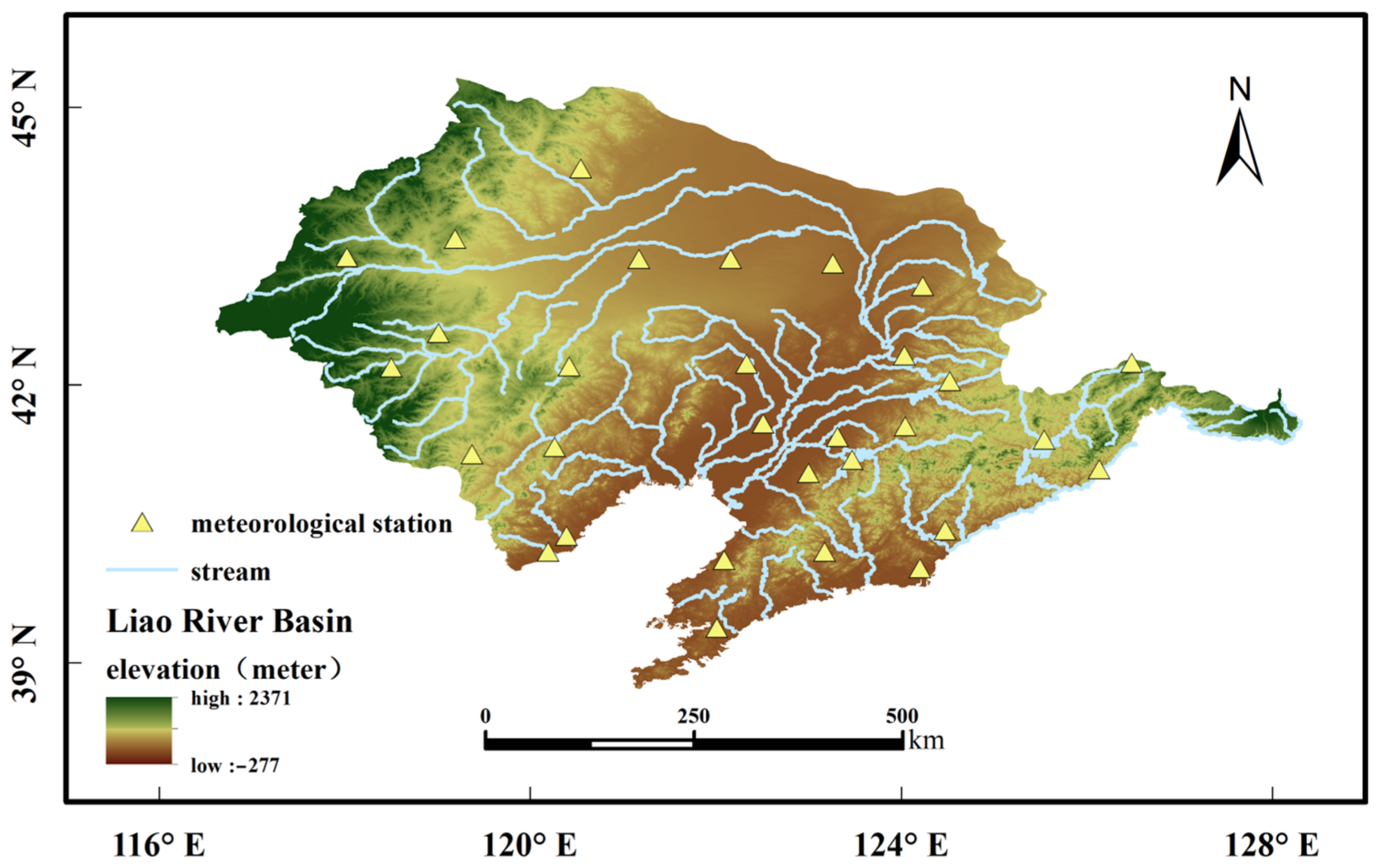
2.1. Research Area

The LRB is located in the southwest of Northeast China and flows through the four provinces (or Autonomous Region) of Hebei, Jilin, Liaoning, and Inner Mongolia into the Bohai Sea, with a total length of 1345 km and a drainage area of 219,000 km². It is one of the seven major rivers in China. The LRB has a semi-humid monsoon climate in most parts. Floods in the basin are frequent, and a large flood occurs every 7–8 years on average. The LRB is becoming a key research objective in the field of climate and hydrology. The range of 116° E–129° E, 38° N–46° N was selected as the research area.

2.2. Data

The precipitation data in the LRB from 1960 to 2020 were obtained from the China Meteorological Data Service Centre (https://data.cma.cn/ (accessed on 18 March 2022)). This study selected the precipitation and temperature records at 30 meteorological stations in the basin. The time series spans nearly 60 years, which ensured the reliability of the analysis and conclusion of this study. The geographic information and meteorological stations of the LRB are shown in Figure 1. The same period of AO and PDO were from the National Oceanic and Atmospheric Administration (http://www.noaa.gov/ (accessed on 5 March 2022)). The Canonical ENSO index dataset was from the UK Met Office’s Hadley Centre (HadISST1). The Annual average of SS relative activity was derived from Solar Influences Data Analysis Center (http://sidc.oma.be/products/meu/index.php (accessed on 5 March 2022)).

2.3. Methodology

To visualize the spatial distribution pattern of precipitation concentration characteristics in the LRB, this study applied the sliding t-test method to identify whether a mutation point existed in the time series of PCP or PCD from 1960 to 2020. The cross-wavelet transform and wavelet coherence analysis methods were used to explore the interaction between precipitation concentration (PCD and PCP) and climate factors.

2.3.1. The PCD and PCP

The calculation method of the PCD and PCP was proposed in 2003 by Zhang and Qian [29]. The PCD is one of the important indicators to evaluate the uniform distribution of regional precipitation in recent years and the PCP could quantitatively reveal the non-uniformity of precipitation in the time field, as shown in previous studies [30,31,32].

The PCD and PCP are calculated as follows:

$$\mathrm{PCD}=\frac{1}{R_i}\sqrt{({\displaystyle \sum }_{j=1}^n{r}_{ij}\times sin{\theta }_j{)}^2+({\displaystyle \sum }_{j=1}^n{r}_{ij}\times cos{\theta }_j{)}^2}$$

(1)

$$\mathrm{PCP}=\arctan (\frac{{{\displaystyle \sum }}_{j=1}^n{r}_{ij}\times sin\theta }{{{\displaystyle \sum }}_{j=1}^n{r}_{ij}\times cos\theta })$$

(2)

• where, n is the total number of days in year i;
• j is the daily ordinal number in year i;
• r_ij is the precipitation of a station in year i on day j;
• R_i is the total precipitation of the station in year i, Divide $\left[-\mathsf{\pi },\mathsf{\pi }\right]$ equally according to the number of days in year i, and θ_j is the azimuth of the jth day.

The PCD value is between 0 and 1. The closer the PCD value is to 1, the more concentrated the annual precipitation. On the contrary, the closer the PCD value is to 0, the more uniform the annual precipitation distribution. In this study, the PCP was converted into a daily ordinal number, which is conducive to the analysis of the period of precipitation concentration intuitively.

2.3.2. Sliding t-Test

The sliding t-test divides a climate series into two subsequences to test the significant difference between the average values of the two subsequences. If the difference between two subsequences exceeds a certain level of significance, it is considered that a mutation has occurred [33].

The function t(n,i) is defined as follows:

$$t\left(n,i\right)=\frac{\left({\overline{x_i}}_2-{\overline{x_i}}_1\right)}{s·\sqrt{\frac{1}{n_1}-\frac{1}{n_2}}}$$

(3)

$$s=\sqrt{\frac{n_1{s}_{i1}^2+n_2{s}_{i2}^2}{n_1+n_2-2}}$$

(4)

where, x_i is the i_th element in the time series, and the sample length n before and after the mutation point can be set artificially to make the test more reliable.

For the time series x_i with n_i sample sizes, a certain time was artificially set as the reference point, and two sub-sequences x_i1 and x_i2 before and after the reference point, with ${\overline{x_i}}_1$ and ${\overline{x_i}}_2$ are the mean values, variances of s_i1² and s_i2² and H: ${\overline{x_i}}_2-{\overline{x_i}}_1=0$, t meets the distribution of (n₁ + n₂ − 2) t; and $\alpha$ is the given significance level (this study takes n₁ = n₂ = 10, α = 0.05). If $\left|t\right|>t_{\alpha }$, then H is false, that means if the mean difference between two sequences exceeds a certain level of significance $t_{\alpha }$, a mutation can be considered to have occurred.

2.3.3. Student t-Test

The student t-test is mainly for small sample sizes (n < 30); if two sets of independent normally distributed samples x₁ and x₂ have different sample numbers n₁ and n₂ and their respective variances s₁² and s₂² are not equal, then the following statistic t-test can be used:

$$t=\frac{{\overline{x_i}}_2-{\overline{x_i}}_1-{\mu }_0}{\sqrt{s_1^2\frac{1}{n_1}+s_2^2\frac{1}{n_2}}}$$

(5)

$$s=\sqrt{\frac{n_1{s}_{i1}^2+n_2{s}_{i2}^2}{n_1+n_2-2}}$$

(6)

where, $\overline{x_1}$ and $\overline{x_2}$ are the mean values. This statistic t follows a t-distribution with confidence df under the null hypothesis H₀: μ₁ − μ₂ = μ₀ is true, where μ₀ is some specified difference that you wish to test. The critical values of t, t_α/2 (α/2 = 0.05) are based on (n₁ + n₂ − 2) df [34].

2.3.4. Cross Wavelet Transform (CWT) Analysis

Meteorological time series have characteristics of randomness, multiple, non-linearity and non-stationarity. CWT method based on wavelet transform can analyze the time-frequency domain fluctuation characteristics of two mutually coupled time series, which combines wavelet coherent (WTC) and cross wavelet power (XWT) analysis. The XWT exposes regions with high common power and further reveals information about the phase relationship [35,36]. In recent years, CWT decomposition has been widely used in the multi-scale analysis of meteorological data [12,37,38,39].

In this method, WX (s) and WY(s) are set as the cross wavelet transform of two-time series X and Y, then the cross wavelet power spectrum is defined as:

$$W_n^{XY}\left(s\right)=W_n^X\left(s\right)W_n^{Y\ast }\left(s\right)$$

(7)

The absolute value of the left term in the above equation is the cross-power spectral density. The larger the absolute value, the higher the correlation. It is assumed that the expected spectra of sequences X and Y are both red noise spectra $P_k^X$ and $P_k^Y$; thus, the cross-wavelet power spectrum distribution relationship can be expressed as follows:

$$\frac{\left|W_n^X\left(s\right)W_n^{Y\ast }\left(s\right)\right|}{{\sigma }_X{\sigma }_Y}=\frac{Z_v\left(P\right)}{v}\sqrt{P_k^X{P}_k^Y}$$

(8)

where, σ_X and σ_Y are the standard deviations of time series X and Y, respectively. The freedom degree (v) of the Morlet wavelet transform is set as 2. When the left term exceeds the upper bound of 95% confidence limit of the power spectrum of red noise, it is considered to pass the test of the standard spectrum of red noise with a significance level of 0.05.

Wavelet coherence transform makes up for the deficiency of cross-wavelet in identifying the correlation between sequences in low-energy regions. The wavelet coherence spectrum of sequences X and Y are defined as follows:

$$R_N^2\left(s\right)=\frac{{\left|S\left(s^{-1}\right)W_n^{YX}\left(s\right)\right|}^2}{S\left(s^{-1}{\left|W_n^Y\left(s\right)\right|}^2\right)·S\left(s^{-1}{\left|W_n^Y\left(s\right)\right|}^2\right)}$$

(9)

where, s is the smoother. In this study, only the parts of the wavelet coherence spectrum whose phase difference $R_N^2\left(s\right)\ge 0.5$ were marked.

3. Results and Discussions

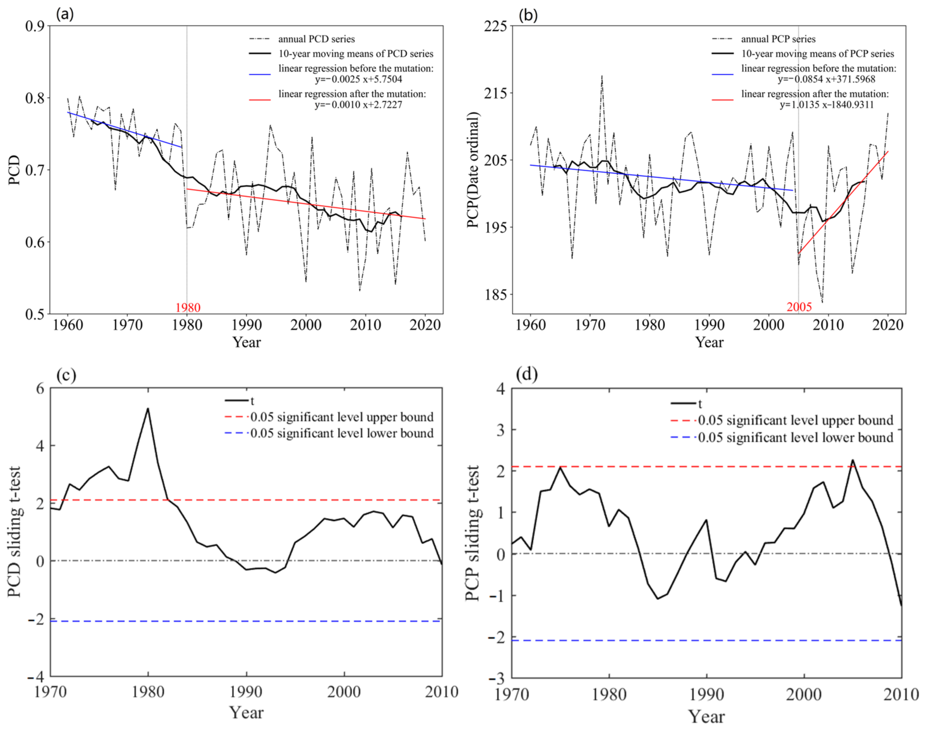
3.1. Mutation Points Identification of the PCD and PCP

The annual average PCD and PCP were calculated in this study based on nearly 60 years of daily precipitation datasets from 30 meteorological stations in the LRB. To make the exploration of secular trends in sequence more convincing, 10-year moving averages were calculated, and the sliding t-test was performed to identify the mutation point of the PCD and PCP sequences (Figure 2).

The results show that the PCD and PCP have different temporal evolution characteristics in the LRB. The variation range of the PCD was between 0.53 and 0.80 during 1960–2020. The mutation of the PCD sequence occurred around 1980 (Figure 2c). The PCD showed a downward trend before and after the mutation. The decrease in the PCD was −0.03/10 a before the mutation (1960–1979), and −0.01/10 a after the mutation (1980–2020). Wang et al. (2019) also pointed out that the annual precipitation concentration of 90% of stations in northeast China showed a downward trend in the period of 1961–2016, and that of 32.39% of stations had a sudden change [11]. The mutation occurred in the PCP sequence around 2005 (Figure 2d). The PCP decreased by −0.09/a before the mutation (1960–2004) and increased by 1.01/a after the mutation (2005–2020).

In the past 60 years, the annual precipitation concentration in the LRB area tended to decrease, which means that the spatial distribution of precipitation tends to be uniform and flattening. After the mutation, the homogenization trend of precipitation distribution was weakened. However, the annual PCP in LRB decreased before 2005, and then increased after the mutation year. In general, the PCP was relatively concentrated, mainly distributed from the 184th to 218th d, that is, from early July to early August.

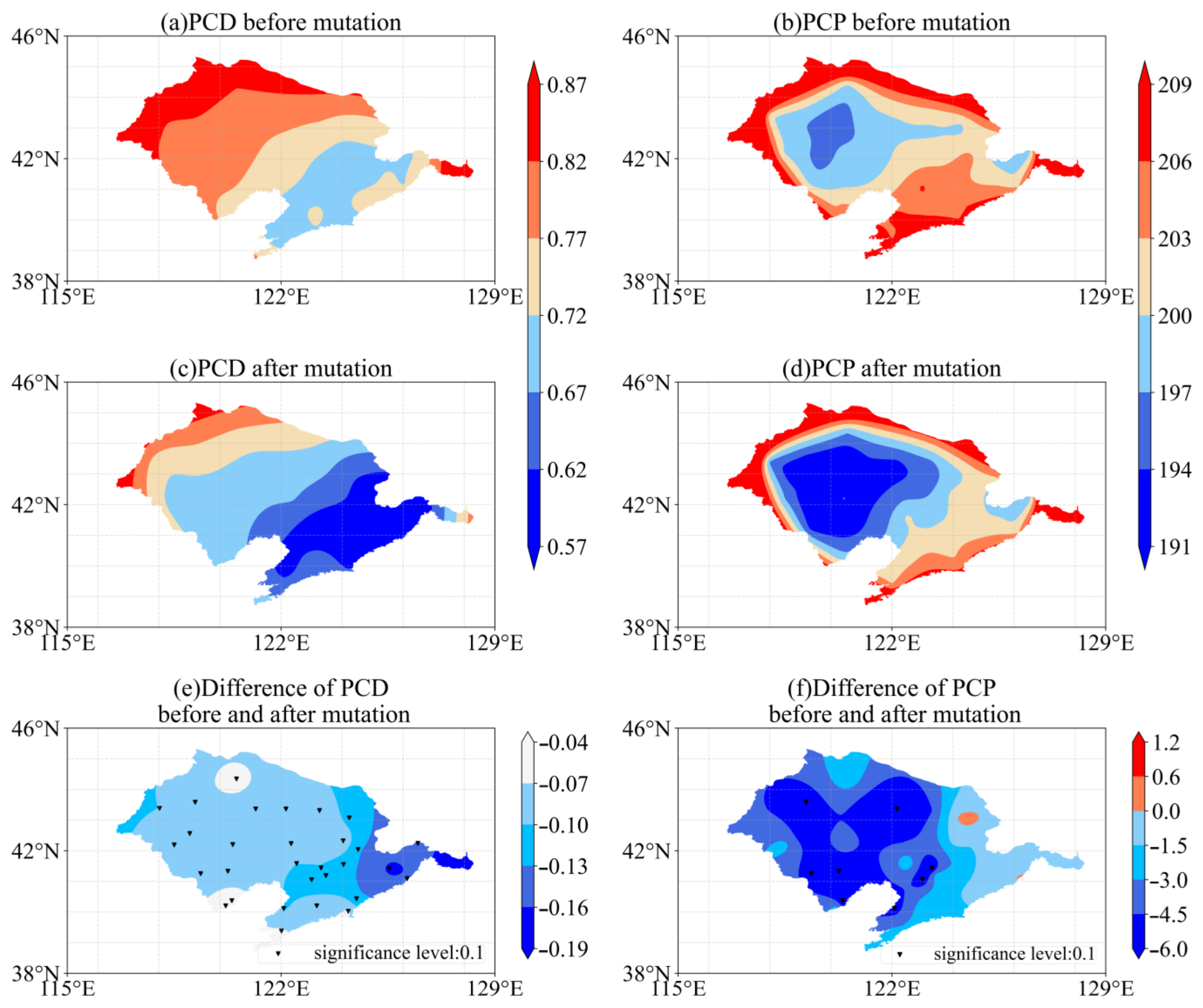
3.2. Spatial Pattern of PCD and PCP

The spatial interpolation method was used to obtain the regional distribution maps of the PCD and the PCP, and the differences before and after the mutation point are compared (Figure 3).

Throughout the study period, the PCD was distributed with high values in the northwest and low values in the southeast in the LRB, as shown in Figure 3a,c. The large value region of PCD (>0.72) was mainly concentrated in the upstream area of the basin and the part of Changchun City in the downstream of the basin. Areas with higher PCD value are at greater risk of storm, flood, and debris flow disasters. In the middle and downstream regions with low PCD values (<0.72), there are more possibilities of drought disasters and dust weather. Figure 3e compares the differences between the PCD before and after the mutation year (1980), and shows that the PCD value decreased significantly, especially in the eastern region, the decrease is up to −0.19, and all stations had passed the significance test. This means that the spatial distribution of precipitation in the whole basin tends to be flat and uniform. Liu et al. (2020) also found that the annual PCI in most areas of the LRB showed an insignificant downward trend from 1960 to 2018, especially in the eastern part of the basin [28].

The spatial distribution characteristics of the PCP were quite different from those of the PCD. Figure 3b,d show that the low values of the PCP (<200th d) were mainly located in the areas to the north of the center of the basin, while the areas with high values of PCP (>204th d) were distributed at the edge of the basin (with the highest values in the northwest and southeast). Figure 3f compares the differences before and after the mutation year (2005) and shows that the PCP decreased (the rains came 0–6 days earlier in the year) in most parts of the basin, but a delayed trend of 1~3 days could still be observed in the northeast corner of the basin. However, only a few stations with the most significant advance trend had passed the significance t-test for the change of PCP. Wang et al. (2019) also found the anomaly of summer precipitation in Northeast China, and they believe that it is driven by changes in atmospheric circulation [11].

Overall, the spatial distribution of annual precipitation in the LRB tended to flatten, and the PCP was slightly earlier after the mutation point. The uniform spatial distribution of precipitation means that the probability of high-level mountain flood and debris flow events is decreasing, and the challenge of source utilization is also decreasing. It is beneficial to human activities. On the other hand, if the precipitation in the main water resource area and the influent area decreases significantly, it would cause further economic losses in the influent area [40]. The detailed analysis of precipitation concentration would help us to make scientific management of water resources in the LRB according to local conditions.

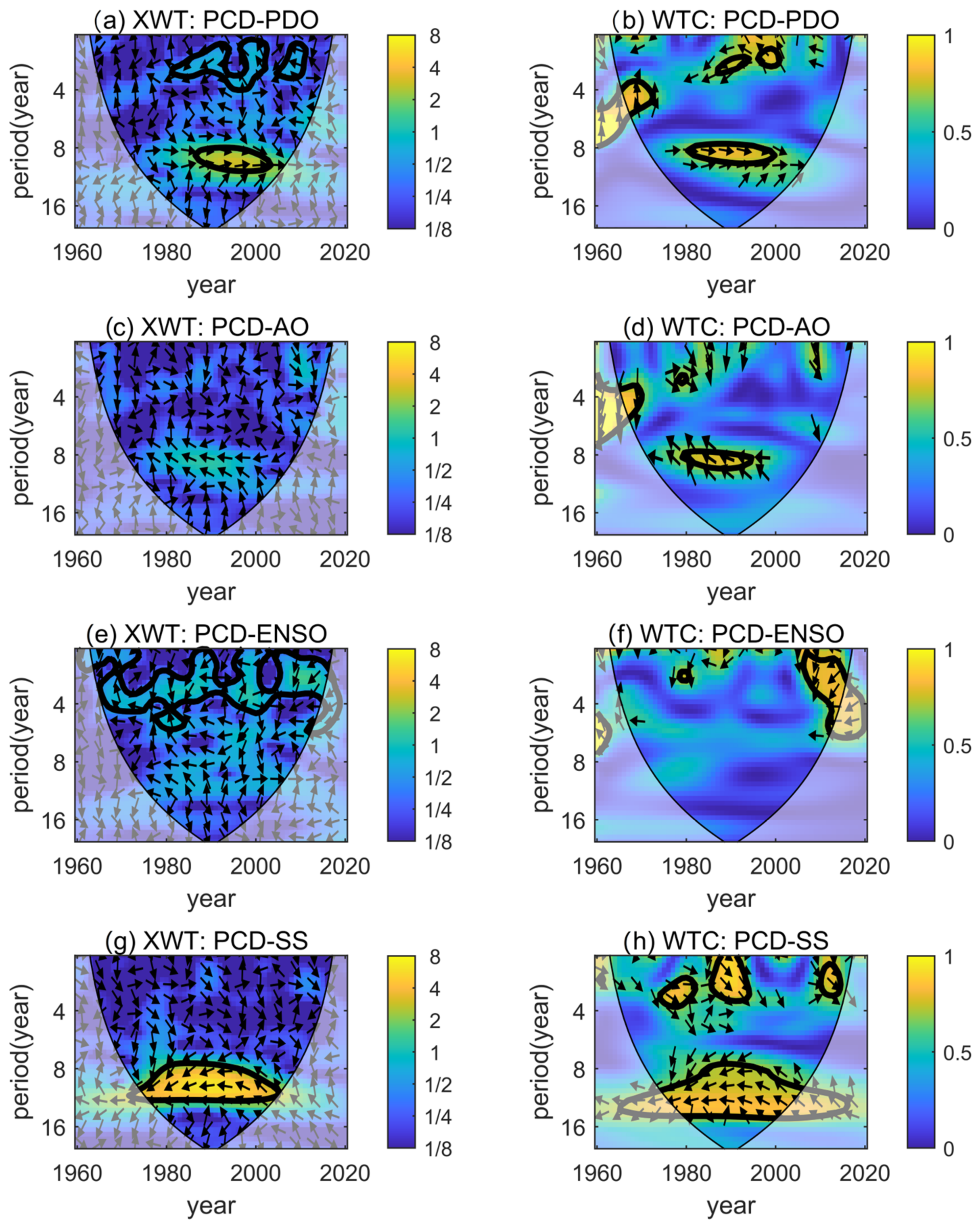
3.3. Relationship between Precipitation Indexes and Low-Frequency Climate Factors

Previous studies showed that low-frequency climate factors have an important impact on regional precipitation [41,42,43,44]. To further explore the influence of the variation of precipitation indexes, CWT analysis was performed on the precipitation concentration sequences (PCD and PCP) and four low-frequency climate factors (PDO, AO, ENSO, and SS), to explore the variation characteristics (such as resonance period, phase relationship and significant period, etc.) between them.

In XWT and WTC power spectrum, the thin black solid line is the influence cone of the wavelet boundary effect. The 5% significance level against red noise is shown as a thick contour. The relative phase relationship is shown as arrows (with in-phase pointing right, anti-phase pointing left, an arrow pointing straight down means the low-frequency climate factor series lags the precipitation index by 90°, and the yellow color represents a high-intensity common period) [35].

3.3.1. PCD

The XWT and the WTC analysis between the PCD and four climate factors are shown in Figure 4. It can be observed from the Figure 4a that multiple resonances between the PCD and PDO exhibited in the high-energy region include two anti-phase resonances with a period of 1–4 a in 1981–2001 and in 2003–2007, separately, and an in-phase resonance with a period of 8–11 a in 1988–2004. In the low-energy region, there are three resonance regions in Figure 4b that include a significant resonance with a period of 3.5–5 a from 1968 to 1974 (PDO leads PCD by nearly 90°), an anti-phase oscillation with a period of 1–3 a from 1988 to 2001, and an in-phase oscillation with a period of 8–10 years from 1980 to 2019.

In the high-energy region, PCD and AO show anti-phase oscillations, respectively, with a period of 3.5–5.5 a (in 1968–1971) and 8–10 a (in 1980–1994) only in the low-energy region in Figure 4d.

The resonance between PCD and ENSO in the high-energy region mainly distributes in the high-frequency domain (with a period of 0–5 a), as is shown in Figure 4e. In the low-energy region, a very significant anti-phase resonance with a period of 1–6 a can be observed from 2006 to 2014 in Figure 4f.

PCD and SS show a significant correlation in the high-energy region between 1974 and 2004 in Figure 4g, that is an anti-phase resonance with a period of 8–12 a. In the low-energy region, three SS lagged in-phase resonance regions can be observed in Figure 4h with a period of 2–3.5 a from 1974 to 1981, a period of 0–3.5 a from 1988 to 1992, and a period of 1–3 a from 2010 to 2012 respectively. In addition, a significant anti-phase vibration with a period of 8–15 a from 1975 to 2005 also can be seen here.

3.3.2. PCP

The XWT and the WTC analysis between the PCP and four climate factors are shown in Figure 5. Between PCP and PDO, it can be observed in Figure 5a that three resonance domains are exhibited in the spectral analysis of XWT. One is a weak in-phase resonance from 1988 to 2005, with a period of 2–6.5 a, one is a PDO ahead anti-phase oscillation from 2008 to 2014, with a period of 5–7 a, the other one is in-phase resonance from 1988 to 2008, with a period of 8–10 a. There are four small resonance domains with PDO ahead dispersed in the map of spectral analysis of WTC in Figure 5b. One of the more significant is in 1963–1968 (with a period of 0–1.5 a), and the others appear in 1981–1988 (with a period of 7 a), in 2008–2009 (with a period of 2 a) and 2009–2011 (with a period of 5.5 a).

Between PCP and AO, it can be obviously seen that an AO ahead anti-phase oscillation exists in 1968–1974 (with a period of 3.5–5.5 a), and a significant AO lagged anti-phase oscillation appears in 1971–1999 (with a period of 3–10 a) in the map of WTC spectrum in Figure 5d.

In Figure 5e, the resonances between PCP and ENSO in the XWT spectrum are all insignificant; three of them exist in 1964–1972 and are in-phase, and the other two exist in 1972–2013 and are anti-phase. In the spectral analysis of WTC for PCP and ENSO in Figure 5f, there is an in-phase synchronization with a period of 0.5–4 a in 1964–1973, and two ENSO ahead anti-phase oscillations can be observed in 1978–1984 and 2009–2013.

In the spectral analysis of XWT of PCP and SS in Figure 5g, it can be observed that the PCP has a significant anti-phase oscillation with SS from 1974 to 2001 with a period of 7.5–14 a. In addition, a small anti-phase oscillation in 2009 with a period of 1.5 a is exhibited in the spectral analysis of XWT in Figure 5h.

Information regarding the resonance phenomenon between PCD and PCP and the four climate factors are summarized in

Table 1. Period and occurrence years of CWT analysis between PCD/PCP and PDO/AO/ENSO/SS.

PCD		XWT		WTC
		Period	Years	Period	Years
	PDO	1–4 a 1–4 a 8–11 a	1981–2001 2003–2007 1988–2004	3.5–5 a 1–3 a 8–10 a	1968–1974 1988–2001 1980–2019
	AO	/	/	3.5–5.5 a 8–10 a	1968–1971 1980–1994
	ENSO	0–5 a	1964–2013	1–6 a	2006–2014
	SS	8–12 a	1973–2003	2–3.5 a 0–3.5 a 1–3 a 8–15 a	1974–1981 1988–1992 2010–2012 1975–2005
PCP		XWT		WTC
		Period	Years	Period	Years
	PDO	2–6 a 5–7 a 8–9 a	1986–2009 2008–2011 1986–2008	0–1.5 a 7 a 2 a 5.5 a	1964–1968 1981–1988 2008–2009 2009–2011
	AO	/	/	3.5–5.5 a 3–10 a	1968–1974 1971–1999
	ENSO	0–4.5 a 1–6 a	1964–1972 1980–2013	0.5–4 a 11–14 a 2–6 a	1964–1973 1978–1984 2009–2013
	SS	7.5–14 a	1974–2001	1.5 a	2009

. The PCD experienced a sudden change around 1980, while the resonance relationship between the three climate factors (PDO, AO, SS) and PCD also changed significantly around 1980. This indicates that climate factors are important reasons driving PCD change, but the resonances between them vary greatly in frequency and phase relationship in different periods. However, the intrinsic mechanism is complex. The effects of PDO and AO on PCD were reflected in the changes of resonance frequency after mutation. The study of Wang et al. (2019) pointed out that PCI is negatively correlated with PDO in the Northeast region [11], but the positive correlation is different at different frequencies in this study. The resonance period of PDO and AO with PCD ranged from 3 to 5 a before the mutation year, but changed (existing in the high-frequency region of 2–3 a and the middle-frequency region of 8–11 a, respectively) after the mutation. The effect of SS on PCD began from 1974, and was enhanced after the mutation year. Regarding PCP, before the mutation year (2005), it was mainly affected by AO and SS, both of them showed anti-phase resonance with PCP, and these two climate factors were slightly delayed. ENSO had different degrees of influence on both PCD and PCP over the entire study period, but there was no correlation with the occurrence of mutations. The correlation between PCP and PDO was not significant. Precipitation indexes (PCD and PCP) had diverse resonance phenomena with low-frequency climatic factors (PDO, AO, ENSO, and SS) at different scales and the differences were obvious before and after mutation.

In the LRB area, SS, PDO, and AO were the important factors driving the abrupt change of the PCD around 1980. Previous studies have also fully confirmed that SS activity has a profound effect on precipitation [44], and the summer precipitation in China increased significantly during the peak of SS activity periods [45]. Rahman and Islam (2019) pointed out that SS is the most important factor affecting the precipitation system, and SS has a negative impact on most precipitation indicators [46]. In this study, it was also found that SS had a negative effect on the PCP and PCD (in the middle and low-frequency domains with a period of 8–15 a), while SS had a positive effect on the PCD in the high-frequency oscillations (with a period of 0–3.5 a) in some years (1974–1981, 1986–1992, 2010–2012). AO showed anti-phase changes with PCD and PCP, while ENSO and PDO had different effects on precipitation indexes at different periods. Zhang et al. (2019) showed that the regional response of the annual precipitation concentration value to the climate factors of the previous 0 years and the previous 1 year was different when the climate factors (ENSO, AO, and PDO) were at different stages [19]. It was also reported that the variation of the PCI is complex and might be related to global atmospheric characteristics and geographical factors. The results of Gong and Wang (2003) indicated that AO has a strong influence on winter precipitation variation in most areas of southern China [47]. Cui et al. (2022) pointed out that the PCD has lagged synchronization with low-frequency climate factors, such as AO and PDO [2].

This study mainly focuses on the correlation and the phase analysis of changes between climate factors and precipitation. However, the climatic dynamics of precipitation are complex and not fully understood. A more comprehensive and quantitative understanding of this system would require more complex analyses, including consideration of a wide range of circulation patterns, or further analysis of ocean–land–atmosphere conditions. How climate factors affect precipitation through atmospheric circulation, and the mechanisms by which they do so, are topics in need of further study.

4. Conclusions

(1)

Mutations occurred in the PCD sequence in 1980 and the PCP sequence in 2005 in the LRB area from 1960 to 2020.

(2)

Over the past 60 years, the annual PCD variation range was between 0.53 and 0.80 and it tended to decrease. The decrease in PCD was −0.03/10 a before the mutation (1960–1979), and −0.01/10 a after the mutation (1980–2020). The PCP decreased by −0.09/a before the mutation (1960–2004) and increased by 1.01/a after the mutation (2005–2020). The daily sequence of PCP in this basin was quite concentrated and ranged from 184th to 218th d, that is, from early July to early August.

(3)

In the LRB, PCD increased from southeast to northwest. Two high PCD (>0.72) areas were concentrated separately in the northwest of the upstream and downstream in Changchun. The spatial distribution of the PCD generally tended to flatten over the entire study period.

(4)

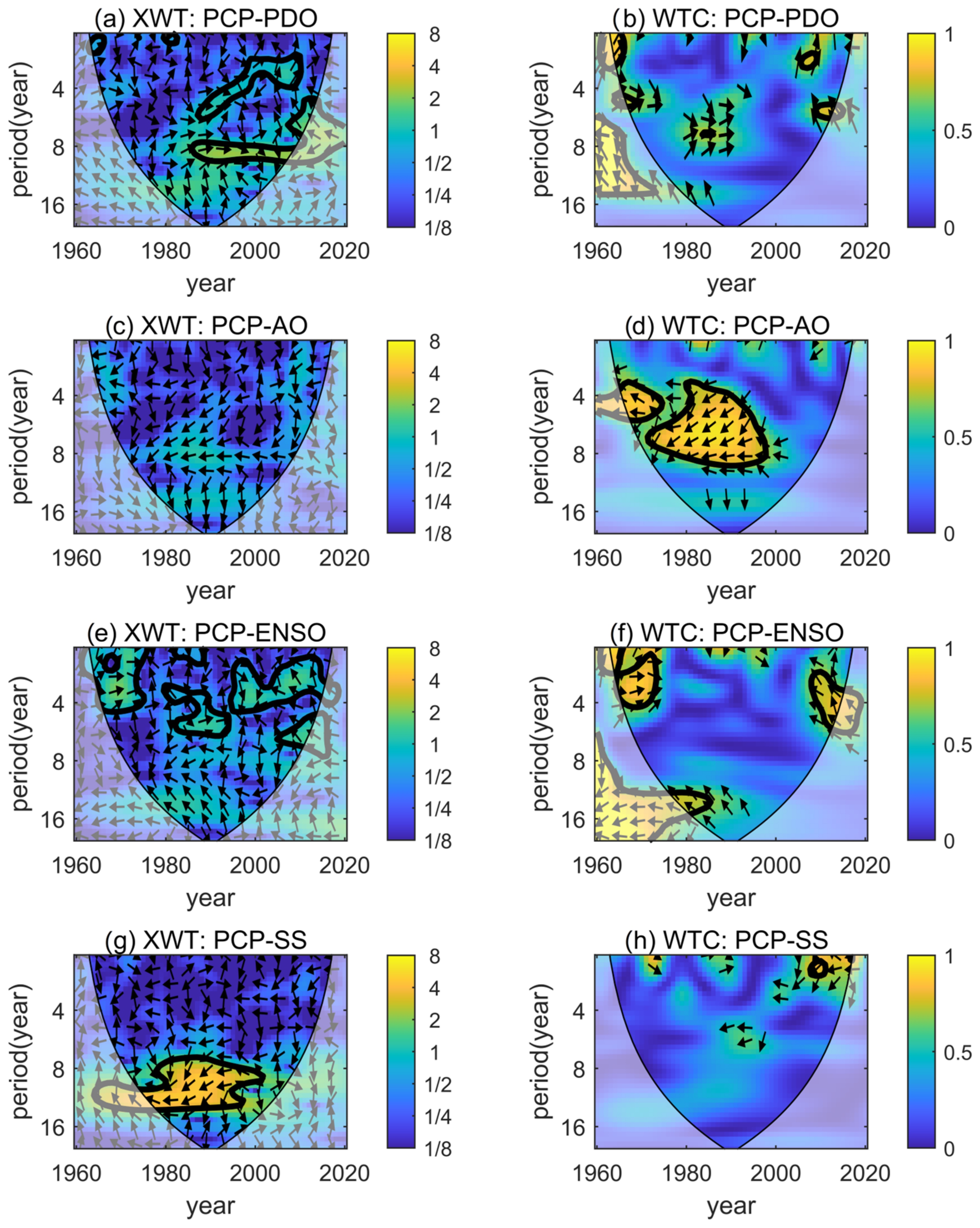
PDO, SS, and AO were the important climate factors driving the abrupt change of PCD, and the resonance between climate factors and the PCD was characterized by complexity and diversity. Before the mutation year 2005, the PCP was mainly affected by AO and SS, both of them showed anti-phase resonance with the PCP, and evolution lagged. ENSO had an important effect on both PCD and PCP but had no significant correlation with the occurrence of the mutations.

References

1. Xie, Z.; Du, Y.; Zeng, Y.; Miao, Q. Classification of yearly extreme precipitation events and associated flood risk in the Yangtze-Huaihe River Valley. Sci. China Earth Sci. 2018, 61, 1341–1356. [Google Scholar] [CrossRef]
2. Cui, H.; Jiang, S.; Ren, L.; Xiao, W.; Yuan, F.; Wang, M.; Wei, L. Dynamics and potential synchronization of regional precipitation concentration and drought-flood abrupt alternation under the influence of reservoir climate. J. Hydrol. Reg. Stud. 2022, 42, 101–147. [Google Scholar] [CrossRef]
3. Zhang, L.; Li, Y.; Zhang, F.; Chen, L.; Pan, T.; Wang, B.; Ren, C. Changes of winter extreme precipitation in Heilongjiang province and the diagnostic analysis of its circulation features. Atmos. Res. 2020, 245, 105094. [Google Scholar] [CrossRef]
4. He, W.; Bu, R.; Xiong, Z.; Hu, Y. Characteristics of temperature and precipitation in Northeastern China from 1961 to 2005. Acta Ecol. Sin. 2013, 33, 519–531. [Google Scholar] [CrossRef]
5. Xie, Y.; Liu, S.; Fang, H.; Ding, M.; Liu, D. A study on the precipitation concentration in a Chinese region and its relationship with teleconnections indices. J. Hydrol. 2022, 612, 128203. [Google Scholar] [CrossRef]
6. Darand, M.; Pazhoh, F. Spatiotemporal changes in precipitation concentration over Iran during 1962–2019. Clim. Change 2022, 173, 25. [Google Scholar] [CrossRef]
7. Liu, Y.; Yan, J.; Cen, M.; Fang, Q.; Liu, Z.; Li, Y. A graded index for evaluating precipitation heterogeneity in China. J. Geogr. Sci. 2016, 26, 673–693. [Google Scholar] [CrossRef] [Green Version]
8. Yin, Y.; Xu, C.-Y.; Chen, H.; Li, L.; Xu, H.; Li, H.; Jain, S.K. Trend and concentration characteristics of precipitation and related climatic teleconnections from 1982 to 2010 in the Beas River basin, India. Glob. Planet. Change 2016, 145, 116–129. [Google Scholar] [CrossRef]
9. Huang, Y.; Wang, H.; Xiao, W.-H.; Chen, L.-H.; Yang, H. Spatiotemporal characteristics of precipitation concentration and the possible links of precipitation to monsoons in China from 1960 to 2015. Theor. Appl. Clim. 2019, 138, 135–152. [Google Scholar] [CrossRef]
10. Sarricolea, P.; Meseguer-Ruiz, Ó.; Serrano-Notivoli, R.; Soto, M.V.; Martin-Vide, J. Trends of daily precipitation concentration in Central-Southern Chile. Atmos. Res. 2019, 215, 85–98. [Google Scholar] [CrossRef]
11. Wang, R.; Zhang, J.; Guo, E.; Zhao, C.; Cao, T. Spatial and temporal variations of precipitation concentration and their relationships with large-scale atmospheric circulations across Northeast China. Atmos. Res. 2019, 222, 62–73. [Google Scholar] [CrossRef]
12. Yang, P.; Zhang, Y.; Xia, J.; Sun, S. Investigation of precipitation concentration and trends and their potential drivers in the major river basins of Central Asia. Atmos. Res. 2020, 245, 105128. [Google Scholar] [CrossRef]
13. Mei, C.; Liu, J.; Huang, Z.; Wang, H.; Wang, K.; Shao, W.; Li, M. Spatiotemporal pattern variations of daily precipitation concentration and their relationship with possible causes in the Yangtze River Delta, China. J. Water Clim. Change 2022, 13, 1583–1598. [Google Scholar] [CrossRef]
14. Gao, L.; Huang, J.; Chen, X.; Chen, Y.; Liu, M. Contributions of natural climate changes and human activities to the trend of extreme precipitation. Atmos. Res. 2018, 205, 60–69. [Google Scholar] [CrossRef]
15. Hao, W.; Shao, Q.; Hao, Z.; Ju, Q.; Baima, W.; Zhang, D. Non-stationary modelling of extreme precipitation by climate indices during rainy season in Hanjiang River Basin, China. Int. J. Clim. 2019, 39, 4154–4169. [Google Scholar] [CrossRef]
16. Zhang, X.; Duan, K.; Dong, Q. Comparison of nonstationary models in analyzing bivariate flood frequency at the Three Gorges Dam. J. Hydrol. 2019, 579, 124208. [Google Scholar] [CrossRef]
17. Yadav, R.K.; Kumar, K.R.; Rajeevan, M. Increasing influence of ENSO and decreasing influence of AO/NAO in the recent decades over northwest India winter precipitation. J. Geophys. Res. Atmos. 2009, 114. [Google Scholar] [CrossRef] [Green Version]
18. Fuentes-Franco, R.; Giorgi, F.; Coppola, E.; Kucharski, F. The role of ENSO and PDO in variability of winter precipitation over North America from twenty first century CMIP5 projections. Clim. Dyn. 2016, 46, 3259–3277. [Google Scholar] [CrossRef]
19. Zhang, K.; Yao, Y.; Qian, X.; Wang, J. Various characteristics of precipitation concentration index and its cause analysis in China between 1960 and 2016. Int. J. Climatol. 2019, 39, 4648–4658. [Google Scholar] [CrossRef]
20. Sun, Q.; Miao, C.; Qiao, Y.; Duan, Q. The nonstationary impact of local temperature changes and ENSO on extreme precipitation at the global scale. Clim. Dyn. 2017, 49, 4281–4292. [Google Scholar] [CrossRef]
21. Zhang, L.; Liu, Y.; Zhan, H.; Jin, M.; Liang, X. Influence of solar activity and EI Niño-Southern Oscillation on precipitation extremes, streamflow variability and flooding events in an arid-semiarid region of China. J. Hydrol. 2021, 601, 126630. [Google Scholar] [CrossRef]
22. Nazari-Sharabian, M.; Karakouzian, M. Relationship between Sunspot Numbers and Mean Annual Precipitation: Application of Cross-Wavelet Transform—A Case Study. J 2020, 3, 67–78. [Google Scholar] [CrossRef] [Green Version]
23. Dong, Q.; Wang, W.; Kunkel, K.E.; Shao, Q.; Xing, W.; Wei, J. Heterogeneous response of global precipitation concentration to global warming. Int. J. Clim. 2021, 41, E2347–E2359. [Google Scholar] [CrossRef]
24. Huan, W.; Er, L.; Wei, Z. A new method to reflect the intra-seasonal heterogeneity of the precipitation in China. J. Trop. Meteorol. 2015, 31, 655–663. [Google Scholar] [CrossRef]
25. Cui, L.; Wang, L.; Lai, Z.; Tian, Q.; Liu, W.; Li, J. Innovative trend analysis of annual and seasonal air temperature and rainfall in the Yangtze River Basin, China during 1960–2015. J. Atmosph. Sol. Terr. Phys. 2017, 164, 48–59. [Google Scholar] [CrossRef]
26. Sangüesa, C.; Pizarro, R.; Ibañez, A.; Pino, J.; Rivera, D.; García-Chevesich, P.; Ingram, B. Spatial and Temporal Analysis of Rainfall Concentration Using the Gini Index and PCI. Water 2018, 10, 112. [Google Scholar] [CrossRef] [Green Version]
27. Cheng, Z.; Chen, X.; Zhang, Y.; Jin, L. Spatio-temporal evolution characteristics of precipitation in the north and south of Qin-ba Mountain area in recent 43 years. Arab. J. Geosci. 2020, 13, 848. [Google Scholar] [CrossRef]
28. Liu, X.; Tong, X.; Jia, Q.; Liu, X.; Xiang, J.; Xue, Z. Characteristics of daily precipitation concentration in Liaohe River Basin from 1960 to 2018. J. Meteorol. Environ. 2020, 36, 18–24. [Google Scholar] [CrossRef]
29. Zhang, L.J.; Qian, Y.P. Annual distribution features of precipitation in China and their interannual variations. Acta Meteorol. Sin. 2003, 146–163. [Google Scholar]
30. Dourado, C.S.; Oliveira, S.R.M.; Avila, A.M.H. Análise de zonas homogêneas em séries temporais de precipitação no Estado da Bahia. Bragantia 2013, 72, 192–198. [Google Scholar] [CrossRef] [Green Version]
31. Silva, B.K.N.; Lucio, P.S. Characterization of risk/exposure to climate extremes for the Brazilian Northeast—Case study: Rio Grande do Norte. Theor. Appl. Clim. 2015, 122, 59–67. [Google Scholar] [CrossRef]
32. Chatterjee, S.; Khan, A.; Akbari, H.; Wang, Y. Monotonic trends in spatio-temporal distribution and concentration of monsoon precipitation (1901–2002), West Bengal, India. Atmos. Res. 2016, 182, 54–75. [Google Scholar] [CrossRef]
33. Du, R.; Shang, F.; Ma, N. Automatic mutation feature identification from well logging curves based on sliding t test algorithm. Clust. Comput. 2019, 22, 14193–14200. [Google Scholar] [CrossRef]
34. Kim, T.K. T test as a parametric statistic. Korean J. Anesthesiol. 2015, 68, 540–546. [Google Scholar] [CrossRef] [Green Version]
35. Grinsted, A.; Moore, J.C.; Jevrejeva, S. Application of the cross wavelet transform and wavelet coherence to geophysical time series. Nonlinear Process. Geophys. 2004, 11, 561–566. [Google Scholar] [CrossRef]
36. Jevrejeva, S.; Moore, J.C.; Grinsted, A. Influence of the Arctic Oscillation and El Niño-Southern Oscillation (ENSO) on ice conditions in the Baltic Sea: The wavelet approach. J. Geophys. Res. Atmos. 2003, 108, 4617. [Google Scholar] [CrossRef] [Green Version]
37. Deng, S.; Chen, T.; Yang, N.; Qu, L.; Li, M.; Chen, D. Spatial and temporal distribution of rainfall and drought characteristics across the Pearl River basin. Sci. Total. Environ. 2018, 619, 28–41. [Google Scholar] [CrossRef]
38. Sun, L.; Cai, Y.; Yang, W.; Yi, Y.; Yang, Z. Climatic variations within the dry valleys in southwestern China and the influences of artificial reservoirs. Clim. Change 2019, 155, 111–125. [Google Scholar] [CrossRef]
39. Li, Q.; Liu, X.; Zhong, Y.; Wang, M.; Shi, M. Precipitation Changes in the Three Gorges Reservoir Area and the Relationship with Water Level Change. Sensors 2021, 21, 6110. [Google Scholar] [CrossRef]
40. Li, C.; Zhang, H.; Singh, V.P.; Fan, J.; Wei, X.; Yang, J.; Wei, X. Investigating variations of precipitation concentration in the transitional zone between Qinling Mountains and Loess Plateau in China: Implications for regional impacts of AO and WPSH. PLoS ONE 2020, 15, e0238709. [Google Scholar] [CrossRef]
41. Trenberth, K.E.; Caron, J.M.; Stepaniak, D.P.; Worley, S. Evolution of El Niño–Southern Oscillation and global atmospheric surface temperatures. J. Geophys. Res. Atmos. 2002, 107, AAC 5-1–AAC 5-17. [Google Scholar] [CrossRef]
42. Dai, A.; Fyfe, J.C.; Xie, S.-P.; Dai, X. Decadal modulation of global surface temperature by internal climate variability. Nat. Clim. Change 2015, 5, 555–559. [Google Scholar] [CrossRef]
43. Dong, B.; Dai, A. The influence of the Interdecadal Pacific Oscillation on Temperature and Precipitation over the Globe. Clim. Dyn. 2015, 45, 2667–2681. [Google Scholar] [CrossRef]
44. Zhang, X.N.; Shi, X.M.; Yang, S.Y. Relationship between number of sunspots and rainfall in Xi’an in summer and autumn. Arid Zone Res. 2013, 30, 485–490. [Google Scholar]
45. Li, H.J.; Gao, J.E.; Zhang, H.C.; Zhang, Y.X. Response of Extreme Precipitation to Solar Activity and El Nino Events in Typical Regions of the Loess Plateau. Adv. Meteorol. 2017, 2017, 9823865. [Google Scholar] [CrossRef] [Green Version]
46. Rahman, M.S.; Islam, A.R.M.T. Are precipitation concentration and intensity changing in Bangladesh overtimes? Analysis of the possible causes of changes in precipitation systems. Sci. Total Environ. 2019, 690, 370–387. [Google Scholar] [CrossRef]
47. Daoyi, G.; Shaowu, W. Influence of Arctic Oscillation on winter climate over China. J. Geogr. Sci. 2003, 13, 208–216. [Google Scholar] [CrossRef]
Figure 1. Map of meteorological station distribution in LRB.
Water 15 00955 g001
Figure 2. Moving t-test schematics of (a) PCD and (b) PCP; (The dashed line is the annual PCD/PCP series, the black solid line is the 10-year moving average, and the blue (red) solid line shows the linear regression before (after) the mutation point) and the t values of (c) PCD and (d) PCP (The black solid lines represent the t-values, and the red (blue) dashed lines represent the 0.05 significance upper (lower) bound).
Water 15 00955 g002
Figure 3. Spatial distribution maps of PCD&PCP: Spatial distribution of (a) PCD and (b) PCP before mutation year; spatial distribution of (c) PCD and (d) PCP after mutation year; differences before and after the mutation of (e) PCD and (f) PCP.
Water 15 00955 g003
Figure 4. CWT spectrum between PCD and PDO/AO/ENSO/SS. (a,c,e,g) show the results of XWT; (b,d,f,h) show the results of WTC.
Water 15 00955 g004
Figure 5. CWT spectrum between PCP and PDO/AO/ENSO/SS. (a,c,e,g) show the results of XWT; (b,d,f,h) show the results of WTC.
Water 15 00955 g005