
A Case Study: Groundwater Level Forecasting of the Gyorae Area in Actual Practice on Jeju Island Using Deep-Learning Technique

1
Department of Hydro Science and Engineering Research, Korea Institute of Civil Engineering and Building Technology, Goyang-Si 10223, Republic of Korea
2
Han River Flood Control Office, Ministry of Environment, Seoul 06501, Republic of Korea
*
Author to whom correspondence should be addressed.
Water 2023, 15(5), 972; https://doi.org/10.3390/w15050972
Submission received: 26 December 2022
/
Revised: 26 February 2023
/
Accepted: 27 February 2023
/
Published: 3 March 2023
(This article belongs to the Special Issue Novel Applications of Surface Water–Groundwater Modeling)
Abstract
:As a significant portion of the available water resources in volcanic terrains such as Jeju Island are dependent on groundwater, reliable groundwater level forecasting is one of the important tasks for efficient water resource management. This study aims to propose deep-learning-based methods for groundwater level forecasting that can be utilized in actual management works and to assess their applicability. The study suggests practical forecasting methodologies through the Gyorae area of Jeju Island, where the groundwater level is highly volatile and unpredictable. To this end, the groundwater level data of the JH Gyorae-1 point and a total of 12 kinds of daily hydro-meteorological data from 2012 to 2021 were collected. Subsequently, five factors (i.e., mean wind speed, sun hours, evaporation, minimum temperature, and daily precipitation) were selected as hydro-meteorological data for groundwater level forecasting through cross-wavelet analysis between the collected hydro-meteorological data and groundwater level data. The study simulated the groundwater level of the JH Gyorae-1 point using the long short-term memory (LSTM) model, a representative deep-learning technique, with the selected data to show that the methodology is adequately applicable. In addition, for its better utilization in actual practice, the study suggests and analyzes (i) a derivatives-based groundwater level learning model which is defined as derivatives-based learning to forecast derivatives (gradients) of the groundwater level, not the target groundwater time series itself, and (ⅱ) an ensemble forecasting methodology in which groundwater level forecasting is performed repetitively with short time intervals.
1. Introduction
Jeju Island is one of the wettest areas in Korea, with the precipitation in normal years being 1142.8–1966.8 mm, with a mean annual precipitation of 1923 mm in the Seogwipo area [1]. However, as most of its ground is covered by volcanic rocks which have high permeability, about 81% of its total water resources depend on groundwater [2]. Against this backdrop, groundwater has been continuously managed by setting a reference groundwater level and taking countermeasures when it is below the threshold [3]. In addition, there have been attempts to efficiently forecast groundwater which have faced lots of difficulties due to Jeju Island’s hydraulic and geological characteristics.
Various methodologies and theories have been proposed for groundwater level (GWL) forecasting, which can be largely categorized into physical-based conceptual models, experimental models, and numerical models [4,5]. The models commonly used for GWL forecasting include MODFLOW [6,7], ISOQUAD [8], HydroGeoSphere [9], and SIMGRO [10,11]. These traditional forecasting models have high efficiency but require lots of input data and involve the process of constructing complex models and calibration to apply analysis methods such as the finite difference method, finite volume method, and finite element method [12]. Moreover, even if a model is constructed and calibrated, due to strong nonlinearity and the high spatial variance of groundwater factors, forecasting the entire system realistically is challenging [13].
As an alternative, data-driven modeling such as machine learning comes to the forefront. The virtue of data-driven modeling is that there is no burden in building various spatial and geological data as it simulates GWL by learning the correlations between GWL and several explanatory variables, and, thus, numerous GWL forecasting studies have utilized it [14]. Around the 2000s, the majority of studies used artificial neural networks. For example, [15] forecasted GWL through an artificial neural network with the data of the groundwater level monitoring network of New Jersey, USA, and [16] utilized an artificial neural network to forecast the groundwater level of the island areas of Greece. Aside from these, many studies employed artificial neural networks for forecasting GWL [17,18,19,20,21]. Since 2010, techniques such as the adaptive network-based fuzzy inference system (ANFIS) [22,23,24,25] and nonlinear autoregressive with external input system (NARX) [26,27,28] have been applied and evaluated to be highly applicable to groundwater management. In addition, since 2018, LSTM-based GWL forecasting that can reflect long-term time series characteristics has emerged thanks to its high simulation efficiency [29,30,31,32,33], while some studies have combined or compared traditional models with deep learning techniques [34,35,36]. Considering precedent studies, deep learning is expected to be applicable to GWL forecasting. However, despite numerous studies having been conducted, GWL forecasting based on deep learning is hard to apply in actual practice due to its uncertainty as a user cannot know how the necessary information is learned and produced [37,38]. Therefore, a pragmatic study for a field engineer considering the uncertainty of deep learning and the decision-making process is needed.
In this regard, the objective of this study is to propose and assess pragmatic methodologies for deep-learning-based GWL forecasting by month to the particular groundwater station in Jeju island and its field engineer. The GWL data of JH Gyorae-1 and a total of 12 types of hydro-meteorological data were collected. Through cross-wavelet and Granger causality analysis between collected hydro-meteorological data and GWL, data were selected for GWL forecasting. Using the selected hydro-meteorological factors, a GWL forecasting model was constructed and analyzed based on the LSTM technique. Furthermore, for application in actual practice, the study suggests (i) derivatives-based learning where GWL is simulated by learning the first derivatives of GWL and (ii) an ensemble forecasting methodology for assisting users to make decisions through multiple models, and it assesses their applicability.
2. Theoretical Background
2.1. Study Material
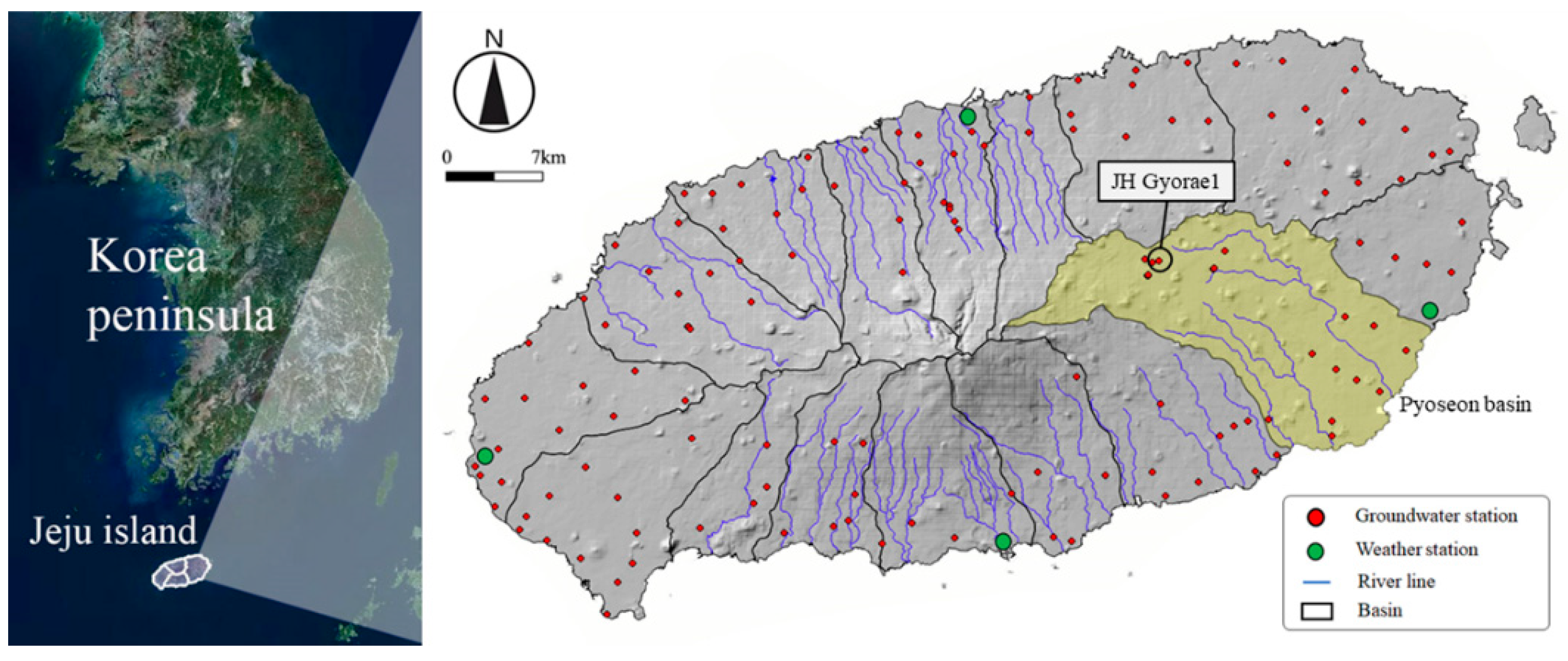
The study subject is the groundwater level of the JH Gyorae-1 point in the hilly and mountainous area of the Pyoseon basin on Jeju Island. Jeju Island is Korea’s representative volcanic island, covered with volcanic rocks and sedimentary rocks originating from igneous rocks. Due to its geological characteristics, its groundwater recharge rate is about 45% and 81% of its total water resources are dependent on groundwater despite its high mean annual precipitation ranging between 1142.8 mm and 1966.8 mm [2]. Accordingly, the local government constructed its groundwater observation network early and has strictly managed groundwater through measures such as the groundwater usage permit system [39]. As of January 2022, there were 135 groundwater level observation wells, 8 artificial recharge observation points, and 12 agricultural water monitoring wells, totaling 155 groundwater observation spots on Jeju Island [1]. Of the 155 spots, the study subject is the GWL of JH Gyorae-1 groundwater observation network in the hilly and mountainous area of the Pyoseon basin in southeastern Jeju Island (Figure 1). Andisols account for 98% of the Pyoseon basin soils, and most of the rivers are dry streams due to the highwater permeability of the soil, so the river water has a negligible impact on the groundwater level [30,40]. The hilly and mountainous area of the Pyoseon basin has thick unsaturated zones, which results in non-linear groundwater properties due to dispersion and lag time [41]. Therefore, when the hydrogeological characteristics such as permeability or recharge rate have not changed much, hydroclimatic factors, including precipitation, are the main factors in determining groundwater level. Moreover, the Gyorae-1 station shows extremely high variability as it changed over 20 m in just 1 month (Figure 1). The Gyorae-1 groundwater monitoring well shows nonlinearity behavior and a high correlation with hydroclimatic factors [30], and it has been determined to be a proper subject for assessing the applicability and forecasting methodologies of LSTM.
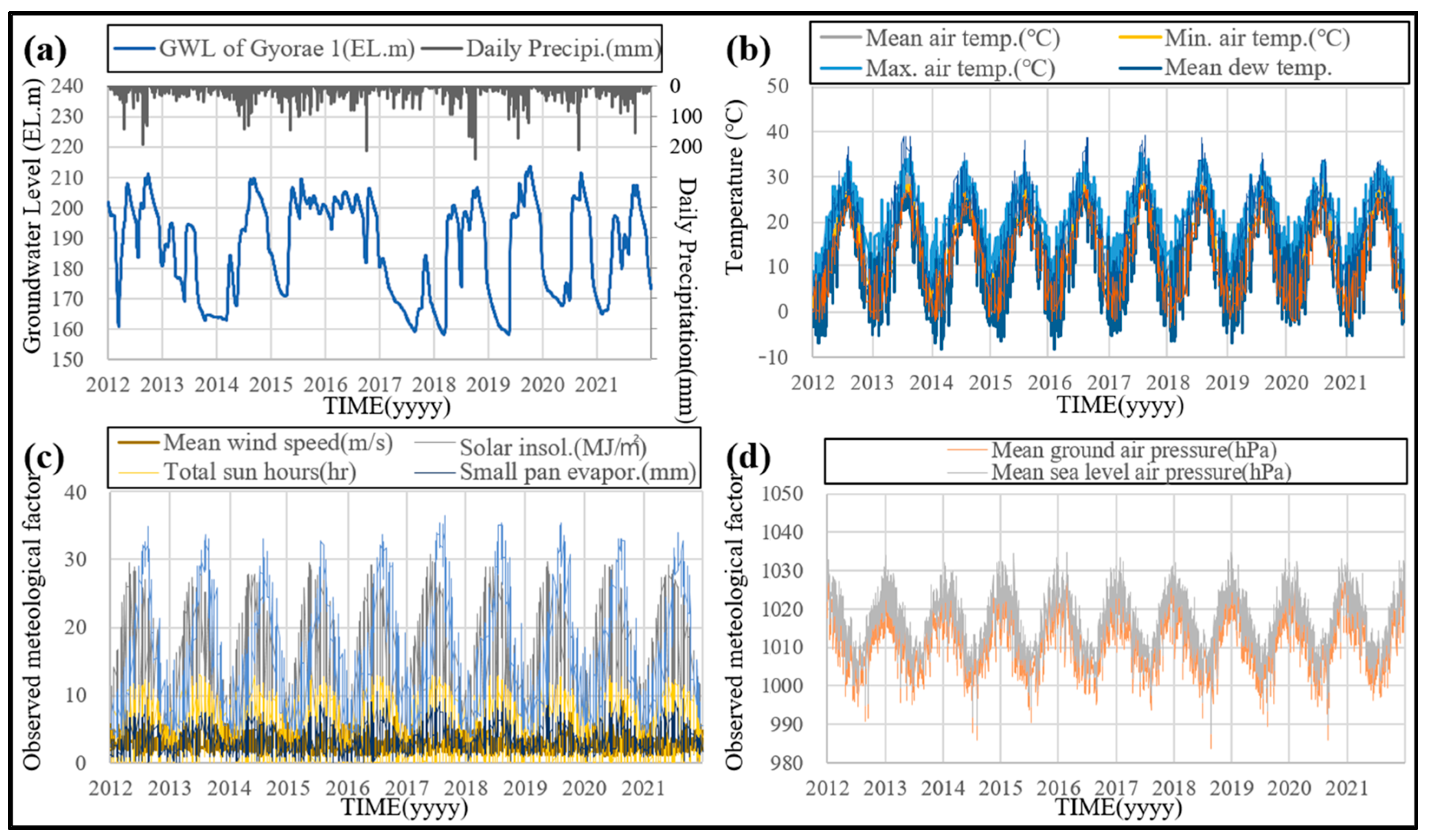
The study needed various hydro-meteorological data from the Pyoseon basin in Jeju and credible GWL observation data from the JH Gyorae-1 point. The data period for this study was set from 2012 to 2021, when reliable data were collected. The hydro-meteorological data used for this study was the Thiessen area weighted means of the data collected from the Automated Synoptic Observing Systems (ASOSs) (Jeju, Seogwipo, Seongsanpo, and Gosan) on Jeju Island. In total, 12 kinds of daily hydro-meteorological data were collected from the Open MET Data Portal of the Korean Meteorological Administration(KMA): daily maximum temperature, daily minimum temperature, daily mean temperature, dew temperature, relative humidity, precipitation, ground air pressure, sea-level pressure, mean wind speed, total sun hours, insolation, and evapotranspiration [42]. The groundwater level data of Gyorae-1 were obtained from the Groundwater Information System of Jeju Special Self-Governing Province [1]. Other materials for this study were acquired from the Soil Groundwater Information System of the National Institute of Environmental Research [43]. In addition, the collected materials were checked for anomalies and erroneous data were eliminated. The obtained materials are shown in Figure 2.
2.2. Test Statistics: Cross-Wavelet and Granger Causality
As this study aims to suggest ways to forecast the groundwater level of Jeju Island using hydro-meteorological data, selecting data that are highly relevant to the groundwater level is a crucial task. To consider the time-sequential correlation between hydro-meteorological data and groundwater level, cross-wavelet analysis and Granger causality were employed. Cross-wavelet analysis is defined as the decomposition and expansion of certain time series into time-frequency space [44]. As a result, periods are separated by time according to the correlation, making it useful to find localized intermittent periodicities [45]. Continuous wavelet transform (CWT) can be defined as:
where is the Morlet wavelet with scale (s) [46], and wavelet power can be defined as . Thus, the cross-wavelet between the two times series and can be represented as , where * denotes complex conjugation. The complex argument of can be interpreted as the phase difference between two times series and Y(t) in the time-frequency space.
Granger causality is a statistical test method used to determine whether the prior values of the independent variable X provide statistically significant information about the future values of dependent variable Y [47]. When the inclusion of X reduces the error of Y in a linear regression model, time-series X would be identified as the cause of Y. Granger causality can be defined by a bivariate autoregressive model as:
where X and Y are each time series, denotes the time step of the time series X and Y, and is the maximum lag in the time series. A and B are the parameters of each autoregressive model, and these are significantly different from zero and can be estimated by the logarithm of the corresponding F-statistic [48]. While being similar to the correlation coefficient, Granger causality allows for the convenient calculation of correlation between two time series and is, therefore, widely utilized in various fields [49].
2.3. LSTM Technique
LSTM [50] was developed during the process of improving recurrent neural networks (RNNs) and is emerging as the current most popular deep learning technique (see Figure 3). Although RNNs are highly efficient in processing time series data, they have problems such as a vanishing gradient from the error slope of long-term data. LSTM was introduced to solve this problem and has shown good results with continuous data such as voice or pattern recognition and translation [51]. LSTM has been used in different areas of hydrology, including not only basin runoff simulation [52,53,54], water level forecasting [55,56], and precipitation forecasting [57,58] but also groundwater level forecasting, where it has produced better outcomes compared to traditional models [29,31,32,33].
The LSTM model incorporates multiple cells, and each cell is constructed to contain the information from the previous timestamp and regulate what information is delivered through gates. The gates are largely divided into 3 types: forget, input, and output gates. These gates determine how much information should be stored, deleted, and delivered to the next cell through the activation function within the hidden layer and execute the delivery of information [51]. The LSTM technique repeats the following six equations with input time series () to calculate output time series ():
where is the non-linear activation function, are the weights of the forget, input, and output gates and memory cell, respectively, and have values between 0 and 1. For example, if is 0, no information is passed on, while if it is 1, complete information is delivered to the next cell. denotes the state of the previous cell’s output, is the current input time series, and are the bias vectors of each gate. In this regard, the LSTM model is free of issues related to long-term time series data and shows high simulation efficiency even with various complex time series. Thus, it is determined as being applicable to a groundwater level that has non-linear and complicated behavior due to thick unsaturated zones, as found in the hilly and mountainous areas in Jeju Island.
3. Application and Proposed New Method
3.1. Predictor Selection for Groundwater Level Forecasting
In forecasting, if a model includes less important variables, the uncertainty of the model increases and the overall forecasting performance is diminished [59]. It also significantly affects the model selection [60]. Moreover, Ref. [61] suggested that predictor selection is even more important than machine learning model selection. Therefore, adequate predictor selection is the key prerequisite for good modeling [59]. Precedent studies [62,63] found that antecedent precipitation has the biggest impact on groundwater level. However, it has been suggested that predictors besides precipitation, such as the thickness of unsaturated zones and the permeability coefficient, influence the change in groundwater level [64,65]. Thus, this study selected optimal influential hydro-meteorological data regarding GWL, based on which a forecasting model was built using deep learning techniques. Although simple user-defined relationships such as traditional coefficients have been used for predictor selection in GWL forecasting, it has been suggested that more considerate non-causal techniques such as discrete wavelet transform (DWT), including time delay, should be considered as well [14]. Indeed, the values of Pearson’s correlation coefficient [66] of the GWL and the hydro-meteorological factors of Gyorae-1 were between −0.05 and 0.36, implying that it is difficult to select predictors based on direct correlation. In particular, predictor selection for Jeju’s GWL is more challenging due to the existence of lag time between antecedent precipitation and the groundwater level [67,68]. Therefore, according to the findings of [14], this study applied cross-wavelet analysis [69] that enables the estimation of temporal correlation between two variables and the Granger causality test [70], which considers the correlation between two time series quantitatively.
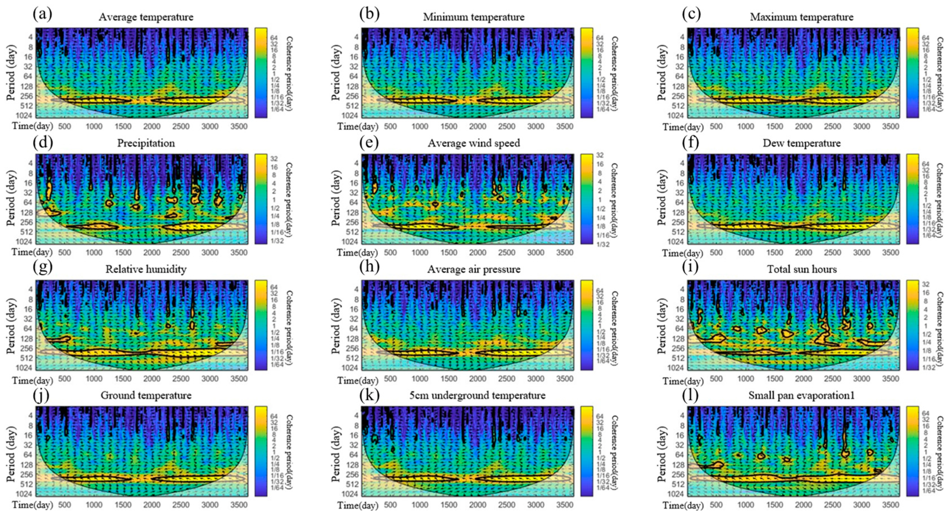
Figure 4 shows the cross-wavelet analysis results where bold-lined areas are the time series determined to have a certain degree of correlation with GWL. Overall, five factors (average wind speed, total sunshine hours, evaporation, minimum temperature, and daily precipitation) seemed to be correlated with GWL. Average wind speed had a high correlation mainly during summer and the correlation lasted for no longer than 1 week. In addition, total sun hours and evaporation showed a correlation mostly during summer and the correlation was maintained for about 2 weeks. The minimum temperature had a correlation throughout the entire period and was especially high except for summer, which lasted for no longer than 1 week. Lastly, daily precipitation showed a high correlation throughout the whole period, which was especially higher during summer and maintained for up to 2 months and thus was determined to be the most influential factor for Gyorae’s GWL. The Granger causality test provided similar results (Table 1). In total, six factors (mean temperature, minimum temperature, precipitation, mean wind speed, total sun hours, and evapotranspiration) showed cross-correlation and were determined to be applicable as input data for deep learning techniques. The correlation between GWL and each hydro-meteorological factor did not appear consistently across the entire period. Rather, it remained weak during ordinary days and the temporal correlation became stronger before and after GWL changed, but it still did not show a consistent correlation. Therefore, deep learning techniques that can derive information desired by users from multidimensional datasets [71] would be a good alternative.
Furthermore, the maximum, average, and minimum temperatures; underground temperature; dew temperature; and relative humidity showed a correlation with GWL as well. According to Table 1, it is safe to say that five kinds of temperatures and relative humidity had a causal relationship with GWL as all of them had values exceeding their corresponding critical values. However, these six items are all meteorological factors related to temperature and, thus, not independent from one another, raising concerns regarding multicollinearity [72]. Therefore, the minimum temperature which showed a correlation throughout the period as well as a high correlation during winter was selected as a correlation factor, while the others were excluded. Consequently, mean wind speed, total sunshine hours, evaporation, minimum temperature, and daily precipitation were chosen as input factors for the LSTM technique in GWL forecasting.
3.2. Construction of the LSTM Model and Result
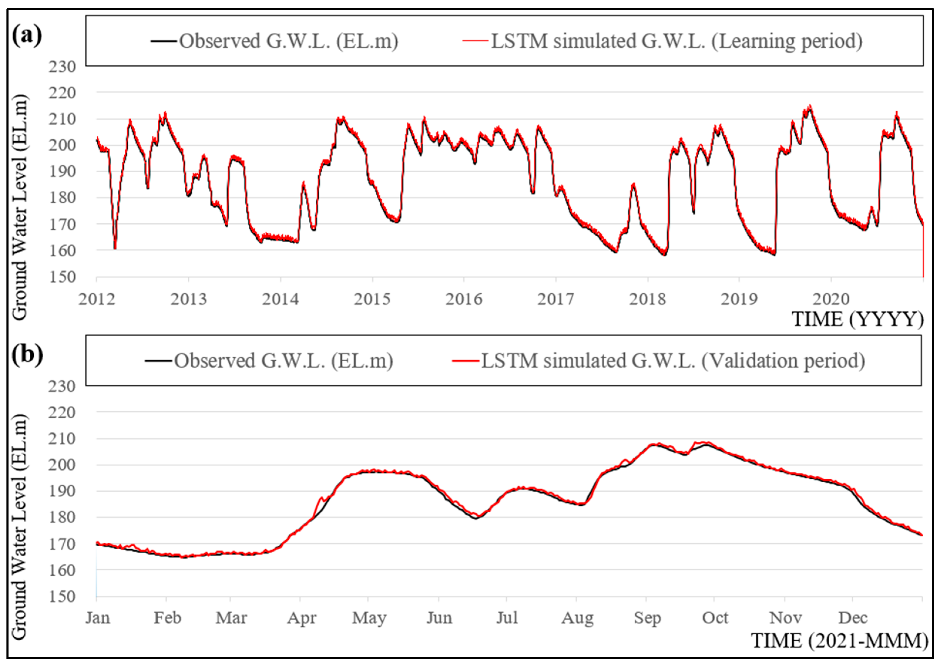
The purpose of this study is to suggest a practical application method for groundwater level forecasting in the groundwater level management field. As hydro-meteorological factors such as precipitation, which has the most dominant influence on groundwater [62,63], are numerically forecasted for up to 6 months, forecasting groundwater using meteorological prediction data is thought to be the most reasonable field application method. To assess its applicability, with the five hydro-meteorological factors selected in the previous section, the LSTM model for simulating the Gyorae-1 area’s GWL as a forecasting result was constructed and reviewed. Since the number of samples of GWL data and the hydro-meteorological data of Gyorae-1 was about 23,000, as per [73], 10 layers were set. Hyperbolic tangent and sigmoid function were used for the activation function to determine the state of cells and gates within layers, while the linear function was used for the activation function of the fully-connected layer. In addition, to avoid the overfitting of the LSTM layer with the fully-connected layer, the dropout rate was set at 10% [74]. The Adam optimizer, which produced good results in previous time series forecasting studies, was chosen for loss function for training the LSTM [75]. The LSTM model described above was trained with five hydro-meteorological factors and GWL data from 2012 to 2020, and the data for the year 2021 were used for validation (see Figure 5).
The simulation result suggests that the LSTM model has extremely high efficiency and good applicability. The coefficient of determination (R2), root mean square error (RMSE, m), and Nash coefficient for determination of the efficiency of hydrological simulation showed high levels at 0.96, 0.02 m, and 0.95, respectively, for the learning period (2012–2020). The same goes for the validation period (2021) with R2, RMSE (m), and the Nash coefficient remaining high at 0.95, 0.03 m, and 0.95, respectively. Its performance was enabled by the fact that deep learning techniques including the LSTM model use a black-box system where learning is conducted automatically from multidimensional datasets [71], and the simulation result proves that it can be applied for solving complex problems such as forecasting groundwater levels. In particular, considering the delay between the antecedent precipitation and the groundwater level in Jeju Island [67,68], the LSTM model which considers temporal correlation may be more suitable for groundwater level simulation. In addition, the LSTM model does not require a separate calculation of lag time. Rather, it considers the correlation and causality between two time series on its own. Therefore, simulating the groundwater level of the Gyorae area through LSTM has enough applicability.
3.3. Proposed New Method to Forecast Groundwater Levels
In the previous section, the groundwater level was simulated using the LSTM model for the JH Gyorae-1 point, and the simulation method was confirmed to have applicability. However, the comprehensive simulation with long-term time series that this study evaluated the efficiency of is somewhat different from how the groundwater level is practically forecasted and managed in the field. The beauty of LSTM is that it utilizes a black-box system where learning is conducted automatically from multidimensional datasets [71]. On the other hand, it also means that a user cannot know how the necessary information is learned and produced. Thus, there is a lack of clarity regarding processes for a particular result in which the way the LSTM model produced a particular result based on certain assumptions and premises is completely unknown, making it difficult for the user to examine the accuracy of the result. In this case, it is challenging for the user to make a decision considering the uncertainty and hence the unclear accountability for the decision that was made [37,38]. As such, [76] argued that, in the field, the hydrological simulation based on deep learning techniques should be used (i) for research purposes or risk analysis only, (ii) with a decision-making process for reviewing or examining the deep-learning-based simulation results, or (iii) with an ethical review on the produced result or a prior social consensus on the accountability for it. For water resources management in Jeju Island, where 81% of available water resources are dependent on groundwater, GWL forecasting in actual practice is essential, and practical measures should be taken according to the forecasts [2]. The problem is that the managers in the field who need to forecast GWLs using deep learning and to perform real actions cannot completely trust deep learning. Therefore, a technique that assists the decision-making process is required for practical application. This section includes a discussion of GWL forecasting in actual practice and suggests clues for future improvement. The deep learning technique is basically a data-driven model, which can be understood as a model where properties are extracted, recognized, and learned from existing data to produce a result [77]. Some studies pointed out that it is technically a kind of interpolation, and, therefore, it is less likely to be applicable for events that are not included in existing data, and its faulty result may bring harmful consequences [76,78]. This section suggests and examines two ways to assist users’ decision-making regarding the above problem: (i) derivatives-based learning and (ii) ensemble forecasting.
The first approach is derivatives-based learning. Some traditional deterministic optimization methods use gradient information instead of series information. The well-known Newton–Raphson method employs function values and derivatives and, thus, is categorized as a gradient-based algorithm. It provides good results for unimodal problems without discontinuity as the usage of derivatives allows for the provision of simplified information on the gradient of the target series [79]. In addition, other previous studies on deep learning pointed out that the provision of selected potential data can reduce learning complexity and enhance efficiency, although the selection of data properties and training of selected data properties can be performed automatically [80]. In a broad sense, GWL forecasting can be regarded as forecasting the gradients of GWL. In this regard, this study assumed that learning the derivatives of groundwater level and excluding other information for forecasting maximizes learning efficiency.
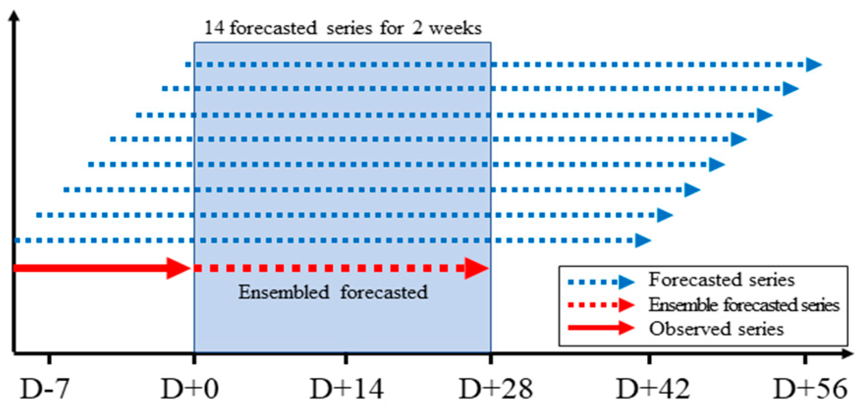
The second approach is ensemble forecasting with the attractor concept. A strange attractor is one of the two most important concepts along with sensitivity to initial conditions in chaos theory [81]. An attractor refers to the continuous changes to move to a state in the natural world and is a concept that refers to the objective state [82]. Given that the GWL changes into a hydrological equilibrium state according to hydrological conditions [83], the equilibrium state of groundwater, where the groundwater changes remain constant according to hydrological conditions, can be regarded as a sort of attractor. Therefore, if a common forecast trend is observed when groundwater level forecasting is performed repetitively with short time intervals, it can be deemed that the future GWL can be determined as following the corresponding forecast, which was defined as ensemble forecasting and its applicability to forecasting was assessed in this study (Figure 6).
The steps were as follows: based on the derivatives-based LSTM model constructed in this section, (i) the GWL changes for one month (D + 28) from each date were forecasted as shown in Figure 7, (ii) the median values of the 14 time series of groundwater forecasted for 2 weeks (D + 14) were utilized as the forecasted groundwater values, and (iii) the forecasted values were compared to the corresponding observed GWLs. In consideration of time series correlation and aging time, the GWL simulation was started 4 weeks prior to each base date and ended 4 weeks (D + 28) after each base date, covering 2 months in total. The simulation period was set as 1 month from each date because the Korea Meteorological Administration currently provides numerical forecasts for 1 month, meaning that the actual forecast data can be acquired from the field. As a result of the simulation, for the 2 weeks from D0, 14 forecasted series in total were produced, and their mean values were used as the forecasted GWLs. However, some time series showing a trend significantly different from that of other time series were regarded as erroneous forecasts and excluded.
4. Result and Discussion
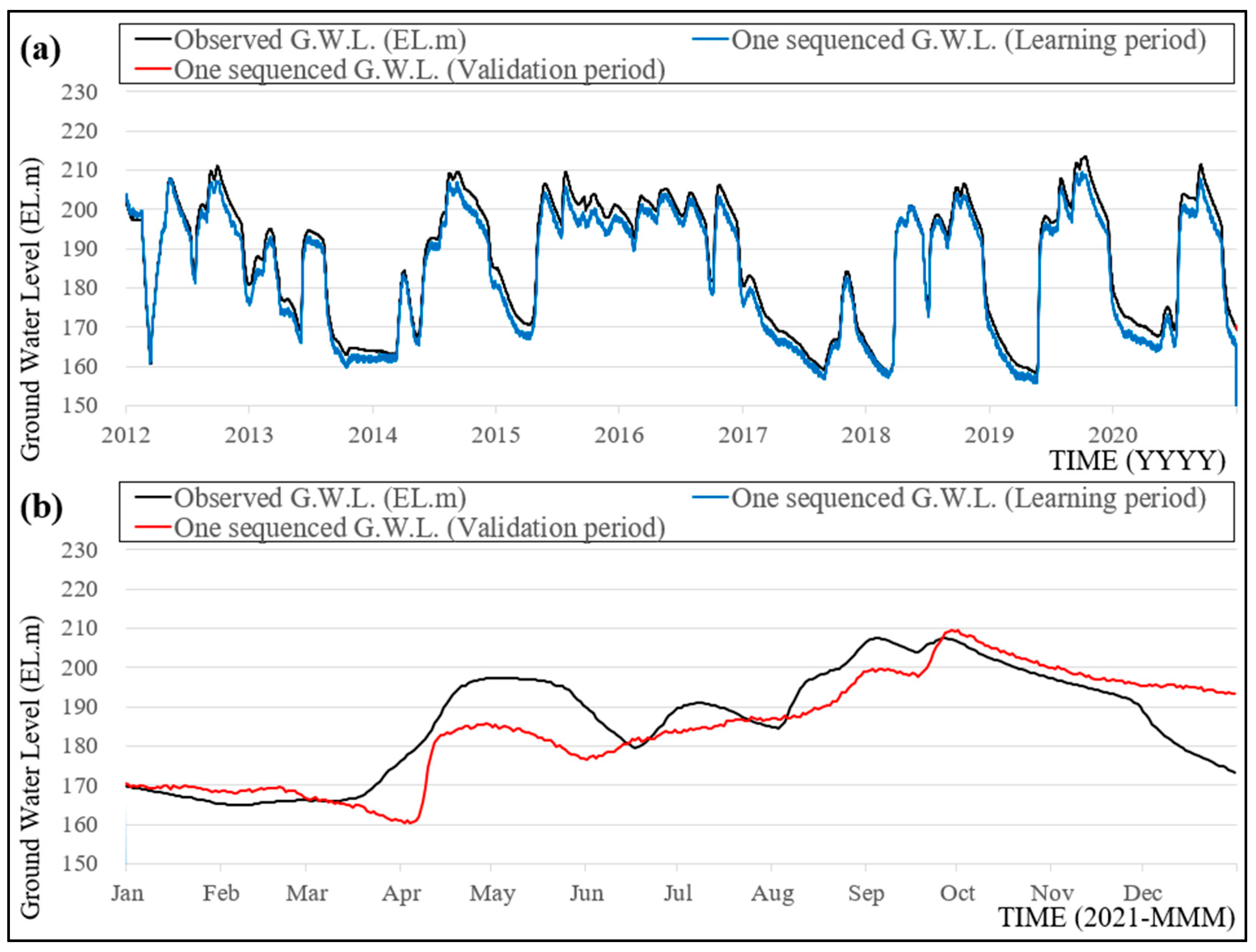
This section analyzes and discusses that suggested in previous section: (i) derivatives-based learning and (ii) ensemble forecasting. For the (i) derivatives-based learning, a new LSTM model for the JH Gyorae-1 point on Jeju Island was trained and constructed through the same process in Section 3.2, using the first derivatives of groundwater time series instead of groundwater data itself. In this case, the gradient of the GWL, not the GWL itself, was the subject of the simulation. To compare the simulation efficiencies, the GWL simulation was based on closed-loop deep learning [84], where only the first observed value of GWL was used and, subsequently, the calculated GWLs from the previous timestamps were regarded as the initial GWL values of the following timestamps. As in the previous section, data from 2012 to 2020 were used for learning, while data for 2021 were utilized for validation (Figure 7).
Based on the simulation result shown in Figure 7, derivatives-based learning is determined to have applicability. R2, RMSE(m), and the Nash coefficient for the learning period in Figure 7 were over 0.62, 8.32 m, and 0.60, respectively. Since, the learning and simulation were performed based on derivatives (gradients) of groundwater time series, not the GWL itself, it can be regarded as the learning and simulation based on the gradients of GWL using hydro-meteorological factors. As the constructed model did not learn GWL in accordance with hydro-meteorological data, it is free from the problem of overfitting to the tendency of the GWL time series [85]. The result of the learning period in Figure 7a indicates that, overall, the model simulated GWL change well. However, although the pattern itself was well simulated, over time, there was a consistent gap between the simulated results and the actual observations. This is attributable to the fact that it was simulated through closed-loop learning after the initial observed value of GWL for the learning and validation periods. As long as the simulation accuracy for GWL change is less than 100%, the gaps at previous time stamps are accumulated, and, consequently, the overall gap increases over time, which can explain the consistent gap shown in Figure 7a. Furthermore, an underestimating tendency of the trained LSTM model can be confirmed from Figure 7a, as well as for the validation in Figure 7b. Although the simulation performance was lower for the validation compared to that of the learning period, the overall pattern was determined to be well simulated. However, there was a certain degree of difference in simulation efficiency as the learning period’s evaluation function was ≥0.9, while that of the validation period was 0.6 for R2 and the Nash coefficient. Therefore, it was determined that overfitting occurred during learning. Nevertheless, even after considering accumulated simulation errors and a certain degree of overfitting from the closed-loop learning, an evaluation function higher than 0.6 signifies that it has sufficient applicability. Moreover, as it can prevent overfitting caused by learning the GWL time series itself, it can be used to validate the results produced by other simulation methods.
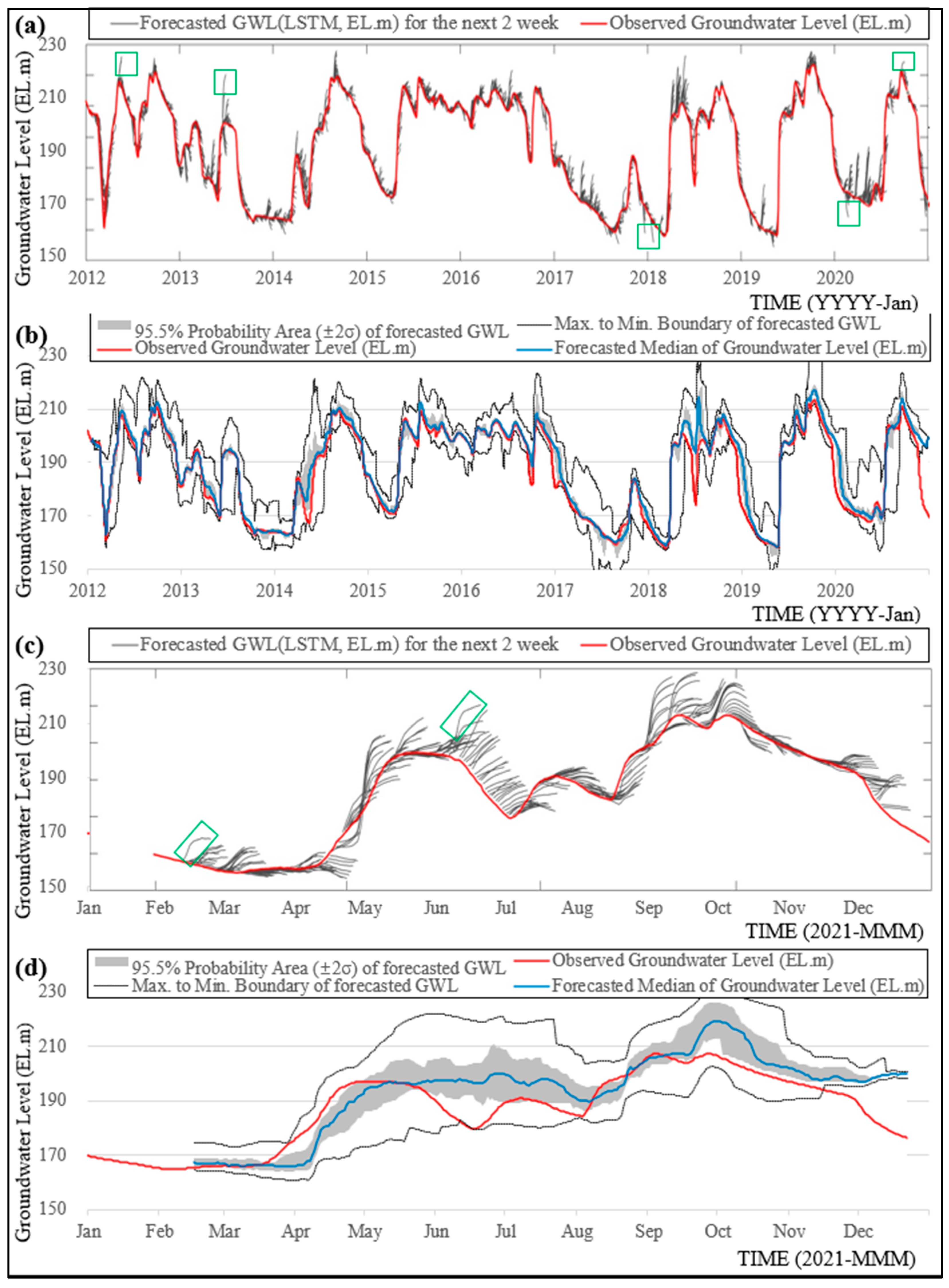
Secondly, for (ii) ensemble forecasting, Figure 8 shows each forecasted series and the ensemble median values produced by ensemble forecasting for the learning period and validation period. Figure 8a,c show multiple forecasting results for 2 weeks (D + 14) from each date (the gray line in Figure 8a,c). Figure 8b,d show the forecasted GWLs (the blue line in Figure 8b,d) according to ensemble forecasting and the 95.5% probability area of forecasted time series (±2σ, the gray boundary in Figure 8b,d). As a result of the comparison between the forecasted values from ensemble forecasting and the observed values, R2, RMSE(m), and the Nash coefficient of the learning period in Figure 8b were 0.92, 2.84 m, and 0.92, respectively, and those of the validation period in Figure 8d were 0.90, 3.95 m, and 0.89, respectively, thus implying that it has applicability.
Ensemble forecasting where the ensemble median values of accumulated time series are used as forecasted values has two merits. Firstly, as it repeats forecasting on a daily basis and uses the mean values of forecasts, the results can be used as basic data for decisions made based on the GWL trend. As it assumes that the future GWL will follow the trend if repetitive GWL forecasting suggests a common trend, its consistent and common forecasts can be significantly helpful for managers in making a decision. Secondly, if a forecasted series of a certain date shows a big difference from others, it can be regarded as erroneous and thus excluded. Indeed, some forecasted series of certain base dates were substantially apart from other neighboring time series (the green box in Figure 8a,c) and were therefore excluded from the estimation of forecasted groundwater level. As such, it can help decrease uncertainty—even psychological uncertainty—when managers forecast GWLs and make decisions. For that reason, derivatives-based learning and ensemble forecasting are determined to be appropriate to complement groundwater forecasting in actual practice. The result of the study could be summarized as follows: the GWL of the single station could be forecasted using the hydro-meteorological factors, and pragmatic application was considered. The suggested methodologies in this study are expected to be a pragmatic method for field engineers.
One of the limitations of this study is that hydro-meteorological factors were used to forecast GWLs. The observed hydro-meteorological data were regarded as forecasted data and used in the simulation. However, in practice, the meteorological data forecasted by the Korean Meteorological Administration is used, and, consequently, the uncertainty of meteorological forecasting is reflected in GWL forecasting. Additionally, its explanation power seems not to be proper in the long-term, such as on a seasonal or yearly scale. Ref. [86] suggested that the probability forecast for temperature was reliable, while that for precipitation was reliable only in a few regions. In this regard, to utilize it in actual practice, the reliability of hydro-meteorological forecasting should be guaranteed to a certain degree. Another limitation is that the derivatives-based learning and attractor-concept ensemble forecasting methods suggested in this study do not theoretically complement deep learning techniques. Still, they should be of value as practical application techniques. There has not been an alternative developed to fundamentally solve the primary problem of deep learning which the study discussed—whether deep-learning-based groundwater forecasting in practice can be credible and used in decision-making. To resolve this issue, a deep learning algorithm should be able to understand and learn about the GWL process conceptually. Therefore, a conceptualized deep learning method needs to be developed. The last limitation is that the study was only applied to single groundwater well. In actual practice, the spatial distribution of groundwater is essential for proper management. Therefore, further studies which apply the forecasting method of the study in a spatial scale are needed.
5. Conclusions
The aim of the study was to propose and assess pragmatic methodologies for deep-learning-based GWL forecasting by month for the JH Gyorae-1 point on Jeju Island, which traditional methods can hardly predict due to its high volatility. To achieve this, the GWL data of JH Gyorae-1 and hydro-meteorological data were obtained to simulate the GWL change and demonstrate that it has applicability to forecasting. Moreover, it proposed (i) derivatives-based GWL learning and (ii) an ensemble forecasting methodology to complement the deep learning results which cannot be used easily for decision-making in actual GWL forecasting and management due to their “lack of clarity of process for a particular result” and analyzed the results. The outcomes of this study can be summarized as follows:
- The study analyzed the correlation between JH Gyorae-1′s GWLs and 12 kinds of hydro-meteorological data (maximum temperature, daily minimum temperature, daily mean temperature, dew temperature, relative humidity, precipitation, ground air pressure, sea-level pressure, mean wind speed, total sun hours, insolation, and evapotranspiration) through cross-wavelet and Granger causality analysis for predictor selection. As a result, five factors (mean wind speed, sun hours, evaporation, minimum temperature, and daily precipitation) showed time sequential correlations with GWLs and were selected as predictors.
- An LSTM model, a representative deep learning method, was constructed using the observed GWLs of JH Gyorae-1 from 2012 to 2020, and the model was validated with the events of the year 2021. The simulation demonstrated a highly outstanding performance and applicability with R2, RMSE(m), and the Nash coefficient, which show the simulation efficiency of a model for its learning and validation periods of ≥0.97, ≤0.03 m, and ≥0.96, respectively.
- It proposed (i) derivatives-based learning and assessed the applicability to complement the lack of clarity of process for a particular result that deep-learning-based forecasts have. An LSTM model was constructed through learning based on the derivatives of GWLs and presented convincing results with R2, RMSE(m), and Nash coefficient of 0.93, 3.92 m, and 0.93, respectively, for the long-term (learning period) simulation, which used only the first observational GWL, and of 0.62, 8.32 m, and 0.60, respectively, for the 1-year validation period (2021). Therefore, it showed that the method can be utilized to aid decision-making when managers review deep learning models.
- It also proposed and assessed (ii) ensemble forecasting. As for ensemble forecasting, ±1-month GWL simulation and forecasting were repeated on a daily basis, and the GWLs for the following 2 weeks were forecasted using the medians of the forecasted time series. The result demonstrated that it is sufficiently applicable as R2, RMSE(m), and the Nash coefficient were, respectively, 0.97, 1.84 m, and 0.97 for the learning period and 0.91, 3.75 m, and 0.90 for the validation period.
Deep learning has become an offer that cannot be refused [87] and it is time to think about the role of deep learning in hydrological practice. In a similar vein, studies on how deep learning can be practically utilized in forecasting or management are urgently needed, and hydrologists should conduct in-depth research on its practical application.
Author Contributions
Conceptualization, D.K. and J.K.; methodology, D.K., J.K., and C.J.; software, C.J. and J.C.; validation, D.K. and J.K.; formal analysis, J.C. and C.J.; investigation, D.K.; resources, C.J.; data curation, J.K. and J.C.; writing—original draft preparation, D.K. and J.K.; writing—review and editing, D.K., J.K., and C.J.; visualization, J.K. and J.C.; supervision, D.K. and J.K.; project administration, D.K.; funding acquisition, D.K. All authors have read and agreed to the published version of the manuscript.
Funding
Research for this paper was carried out under the KICT Research Program (project no. 20230155-001, Development of future-leading technologies solving water crisis against to water disasters affected by climate change) funded by the Ministry of Science and ICT.
Institutional Review Board Statement
Not applicable.
Informed Consent Statement
Not applicable.
Data Availability Statement
Not applicable.
Conflicts of Interest
The authors declare no conflict of interest.
References
- Jeju Special Self-Governing Province. Groundwater Information System. Available online: https://water.jeju.go.kr/JWR/pStatus.cs (accessed on 30 December 2022).
- Korea Water Resources Corporation. Comprehensive Water Resources Management Plan in Jeju Island; Jeju Special Self-Governing Province (JSSGP): Jeju, Republic of Korea, 2018; pp. 1–328. [Google Scholar]
- Kim, J.W.; Koh, G.W.; Won, J.H.; Han, C. A Study on the Determination of Management Groundwater Level on Jeju Island. J. KoSSGE 2005, 10, 12–19. (In Korean) [Google Scholar]
- Izady, A.; Davary, K.; Alizadeh, A.; Ziaei, A.N.; Alipoor, A.; Joodavi, A.; Brusseau, M.L. A framework toward developing a groundwater conceptual model. Arab. J. Geosci. 2013, 7, 3611–3631. [Google Scholar] [CrossRef]
- Xue, J.; Huo, Z.; Wang, F.; Kang, S.; Huang, G. Untangling the effects of shallow groundwater and deficit irrigation on irrigation water productivity in arid region: New conceptual model. Sci. Total Environ. 2018, 619, 1170–1182. [Google Scholar] [CrossRef]
- Dehghani, A. Numerical simulation of groundwater level using MODFLOW software (a case study: Narmab watershed, Golestan province). Int. J. Adv. Biol. Biomed. Res. 2013, 1, 858–873. [Google Scholar]
- Chakraborty, S.; Maity, P.K.; Das, S. Investigation, simulation, identification and prediction of groundwater levels in coastal areas of Purba Midnapur, India, using MODFLOW. Environ. Dev. Sustain. 2019, 22, 3805–3837. [Google Scholar] [CrossRef]
- Yang, C.-C.; Chang, L.-C.; Chen, C.-S.; Yeh, M.-S. Multi-objective Planning for Conjunctive Use of Surface and Subsurface Water Using Genetic Algorithm and Dynamics Programming. Water Resour. Manag. 2008, 23, 417–437. [Google Scholar] [CrossRef]
- Brunner, P.A.; Simmons, C.T. HydroGeoSphere: A Fully Integrated, Physically Based Hydrological Model. Ground Water 2011, 50, 170–176. [Google Scholar] [CrossRef] [Green Version]
- Van Walsum, P.; Veldhuizen, A. Integration Of Models Using Shared State Variables: Implementation In The Regional Hydrologic Modelling System SIMGRO. J. Hydrol. 2011, 409, 363–370. [Google Scholar] [CrossRef]
- Kurniawan, B.; Tapriziah, E.R.; Aryantie, M.H.; Rahmani, R.; Purnomo, A.D. Application of groundwater modeling to predict the effectiveness of various peat dome restoration methods in Pulang Pisau District, Central Kalimantan Province. In Proceedings of the IOP Conference Series: Earth and Environmental Science, Proceedings of 2021 The 6th International Conference of Indonesia Forestry Researchers—Stream 1 Emerging Environmental Quality for Better Living, Tangerang, Indonesia, 8 September 2021; IOP Publishing: Bristol, UK, 2021; Volume 909, p. 012004. [Google Scholar]
- Tao, H.; Hameed, M.M.; Marhoon, H.A.; Zounemat-Kermani, M.; Heddam, S.; Kim, S.; Sulaiman, S.O.; Tan, M.L.; Sa’Adi, Z.; Mehr, A.D.; et al. Groundwater level prediction using machine learning models: A comprehensive review. Neurocomputing 2022, 489, 271–308. [Google Scholar] [CrossRef]
- Sahoo, S.; Russo, T.A.; Elliott, J.; Foster, I. Machine learning algorithms for modeling groundwater level changes in agricultural regions of the U.S. Water Resour. Res. 2017, 53, 3878–3895. [Google Scholar] [CrossRef] [Green Version]
- Rajaee, T.; Ebrahimi, H.; Nourani, V. A review of the artificial intelligence methods in groundwater level modeling. J. Hydrol. 2019, 572, 336–351. [Google Scholar] [CrossRef]
- Coppola, E.A., Jr.; Rana, A.J.; Poulton, M.M.; Szidarovszky, F.; Uhl, V.W. A neural network model for predicting aquifer water level elevations. Ground Water 2005, 43, 231–241. [Google Scholar] [CrossRef] [PubMed]
- Daliakopoulos, I.N.; Coulibaly, P.; Tsanis, I.K. Groundwater level forecasting using artificial neural networks. J. Hydrol. 2005, 309, 229–240. [Google Scholar] [CrossRef]
- Krishna, B.; Rao, Y.R.S.; Vijaya, T. Modelling groundwater levels in an urban coastal aquifer using artificial neural networks. Hydrol. Process 2007, 22, 1180–1188. [Google Scholar] [CrossRef]
- Rakhshandehroo, G.R.; Vaghefi, M.; Aghbolaghi, M.A. Forecasting Groundwater Level in Shiraz Plain Using Artificial Neural Networks. Arab. J. Sci. Eng. 2012, 37, 1871–1883. [Google Scholar] [CrossRef]
- Taormina, R.; Chau, K.-W.; Sethi, R. Artificial neural network simulation of hourly groundwater levels in a coastal aquifer system of the Venice lagoon. Eng. Appl. Artif. Intell. 2012, 25, 1670–1676. [Google Scholar] [CrossRef] [Green Version]
- Jha, M.K.; Sahoo, S. Efficacy of neural network and genetic algorithm techniques in simulating spatio-temporal fluctuations of groundwater. Hydrol. Process 2014, 29, 671–691. [Google Scholar] [CrossRef]
- Chitsazan, M.; Rahmani, G.; Neyamadpour, A. Forecasting groundwater level by artificial neural networks as an alternative approach to groundwater modeling. J. Geol. Soc. India 2015, 85, 98–106. [Google Scholar] [CrossRef]
- Djurovic, N.; Domazet, M.; Stričević, R.; Pocuca, V.; Spalevic, V.; Pivic, R.; Gregoric, E.; Domazet, U. Comparison of Groundwater Level Models Based on Artificial Neural Networks and ANFIS. Sci. World J. 2015, 2015, 1–13. [Google Scholar] [CrossRef] [Green Version]
- Mirzavand, M.; Khoshnevisan, B.; Shamshirband, S.; Kişi, O.; Ahmad, R.; Akib, S. RETRACTED ARTICLE: Evaluating groundwater level fluctuation by support vector regression and neuro-fuzzy methods: A comparative study. Nat. Hazards 2015, 102, 1611–1612. [Google Scholar] [CrossRef]
- Nourani, V.; Mousavi, S. Spatiotemporal groundwater level modeling using hybrid artificial intelligence-meshless method. J. Hydrol. 2016, 536, 10–25. [Google Scholar] [CrossRef]
- Salari, S.; Moghaddasi, M.; Ghaleni, M.M.; Akbari, M. Groundwater level prediction in Golpayegan aquifer using ANFIS and PSO combination. Iran. J. Soil Water Res. 2021, 5, 721–732. [Google Scholar]
- Chang, F.-J.; Chang, L.-C.; Huang, C.-W.; Kao, I.-F. Prediction of monthly regional groundwater levels through hybrid soft-computing techniques. J. Hydrol. 2016, 541, 965–976. [Google Scholar] [CrossRef]
- Di Nunno, F.; Granata, F. Groundwater level prediction in Apulia region (Southern Italy) using NARX neural network. Environ. Res. 2020, 190, 110062. [Google Scholar] [CrossRef] [PubMed]
- Wunsch, A.; Liesch, T.; Broda, S. Forecasting groundwater levels using nonlinear autoregressive networks with exogenous input (NARX). J. Hydrol. 2018, 567, 743–758. [Google Scholar] [CrossRef]
- Zhang, J.; Zhu, Y.; Zhang, X.; Ye, M.; Yang, J. Developing a Long Short-Term Memory (LSTM) based model for predicting water table depth in agricultural areas. J. Hydrol. 2018, 561, 918–929. [Google Scholar] [CrossRef]
- Shin, M.-J.; Moon, S.-H.; Kang, K.; Moon, D.-C.; Koh, H.-J. Analysis of Groundwater Level Variations Caused by the Changes in Groundwater Withdrawals Using Long Short-Term Memory Network. Hydrology 2020, 7, 64. [Google Scholar] [CrossRef]
- Vu, M.; Jardani, A.; Massei, N.; Fournier, M. Reconstruction of missing groundwater level data by using Long Short-Term Memory (LSTM) deep neural network. J. Hydrol. 2020, 597, 125776. [Google Scholar] [CrossRef]
- Solgi, R.; Loáiciga, H.A.; Kram, M. Long short-term memory neural network (LSTM-NN) for aquifer level time series forecasting using in-situ piezometric observations. J. Hydrol. 2021, 601, 126800. [Google Scholar] [CrossRef]
- Lu, C.; Sun, L.; Lu, J. Spatiotemporal forecasting for groundwater level using a WT-LSTM model, In EGU General Assembly Conference Abstracts. In Proceedings of the EGU General Assembly 2020, Online, 4–8 May 2020; p. 6343. [Google Scholar]
- Moghaddam, H.K.; Moghaddam, H.K.; Kivi, Z.R.; Bahreinimotlagh, M.; Alizadeh, M.J. Developing comparative mathematic models, BN and ANN for forecasting of groundwater levels. Groundw. Sustain. Dev. 2019, 9, 100237. [Google Scholar] [CrossRef]
- Malekzadeh, M.; Kardar, S.; Shabanlou, S. Simulation of groundwater level using MODFLOW, extreme learning machine and Wavelet-Extreme Learning Machine models. Groundw. Sustain. Dev. 2019, 9, 100279. [Google Scholar] [CrossRef]
- Zeydalinejad, N. Artificial neural networks vis-à-vis MODFLOW in the simulation of groundwater: A review. Model. Earth Syst. Environ. 2022, 8, 2911–2932. [Google Scholar] [CrossRef]
- Orr, W.; Davis, J.L. Attributions of ethical responsibility by Artificial Intelligence practitioners. Inf. Commun. Soc. 2020, 23, 719–735. [Google Scholar] [CrossRef]
- Campolo, A.; Crawford, K. Enchanted Determinism: Power without Responsibility in Artificial Intelligence. Engag. Sci. Technol. Soc. 2020, 6, 1–19. [Google Scholar] [CrossRef] [Green Version]
- Chung, I.M.; Lee, J.; Chang, S.W. Long-term prediction of groundwater level in Jeju Island using artificial neural network model. KSCE J. Civ. Environ. Eng. Res. 2017, 37, 981–987. [Google Scholar]
- Kang, K.G. Studies on the Hydrogeochemical Processes and Characteristics of Groundwater in the Pyoseon Watershed, Jeju Province. Ph.D. Thesis, Jeju National University, Jeju, Republic of Korea, 2010. [Google Scholar]
- Kim, S.-G.; Koo, M.-H.; Chung, I.-M. Development of a Transient Groundwater Flow Model in Pyoseon Watershed of Jeju Island: Use of a Convolution Method. J. Environ. Sci. Int. 2015, 24, 481–494. [Google Scholar] [CrossRef] [Green Version]
- National Climate Data Center (NDCD). Open MET Data Portal, Korea Meteorological Administration, Seoul, Korea. Available online: https://data.kma.go.kr/cmmn/main.do (accessed on 31 December 2022).
- National Institute of Environmental Research (NIER). Soil Groundwater Information System, Incheon, Korea. Available online: https://sgis.nier.go.kr/web (accessed on 31 December 2022).
- Jevrejeva, S.; Moore, J.C.; Grinsted, A. Influence of the Arctic Oscillation and El Niño-Southern Oscillation (ENSO) on ice conditions in the Baltic Sea: The wavelet approach. J. Geophys. Res. Atmos. 2003, 108. [Google Scholar] [CrossRef] [Green Version]
- Grinsted, A.; Moore, J.C.; Jevrejeva, S. Application of the cross wavelet transform and wavelet coherence to geophysical time series. Nonlinear Process Geophys. 2004, 11, 561–566. [Google Scholar] [CrossRef]
- Lin, J.; Qu, L. Feature extraction based on morlet wavelet and its application for mechanical fault diagnosis. J. Sound Vib. 2000, 234, 135–148. [Google Scholar] [CrossRef]
- Granger, C.W.J. Investigating Causal Relations by Econometric Models and Cross-spectral Methods. Econometrica 1969, 37, 424–438. [Google Scholar] [CrossRef]
- Ding, M.; Chen, Y.; Bressler, S. Granger Causality: Basic Theory and Application to Neuroscience. In Handbook of Time Series Analysis; Schelter, B., Winterhalder, M., Timmer, J., Eds.; John and Wiley and Sons: Wienheim, Germany, 2006; ISBN 978-352-740-623-4. [Google Scholar]
- Granger, C.W.J. Essays in Econometrics: The Collected Papers of Clive W.J. Granger, 1st ed.; Cambridge University Press: Cambridge, UK, 2001; ISBN 978-354-071-334-0. [Google Scholar]
- Hochreiter, S.; Schmidhuber, J. Long short-term memory. Neural Comput. 1997, 9, 1735–1780. [Google Scholar] [CrossRef]
- Yu, Y.; Cao, J.; Zhu, J. An LSTM Short-Term Solar Irradiance Forecasting Under Complicated Weather Conditions. IEEE Access 2019, 7, 145651–145666. [Google Scholar] [CrossRef]
- Feng, R.; Fan, G.; Lin, J.; Yao, B.; Guo, Q. Enhanced Long Short-Term Memory Model for Runoff Prediction. J. Hydrol. Eng. 2021, 26, 04020063. [Google Scholar] [CrossRef]
- Xiang, Z.; Yan, J.; Demir, I. A rainfall-runoff model with LSTM-based sequence-to-sequence learning. Water Resour. Res. 2020, 56, e2019WR025326. [Google Scholar] [CrossRef]
- Gauch, M.; Kratzert, F.; Klotz, D.; Nearing, G.; Lin, J.; Hochreiter, S. Rainfall–runoff prediction at multiple timescales with a single Long Short-Term Memory network. Hydrol. Earth Syst. Sci. 2021, 25, 2045–2062. [Google Scholar] [CrossRef]
- Hrnjica, B.; Bonacci, O. Lake Level Prediction using Feed Forward and Recurrent Neural Networks. Water Resour. Manag. 2019, 33, 2471–2484. [Google Scholar] [CrossRef]
- Kardhana, H.; Valerian, J.R.; Rohmat, F.I.W.; Kusuma, M.S.B. Improving Jakarta’s Katulampa Barrage Extreme Water Level Prediction Using Satellite-Based Long Short-Term Memory (LSTM) Neural Networks. Water 2022, 14, 1469. [Google Scholar] [CrossRef]
- Tao, L.; He, X.; Li, J.; Yang, D. A multiscale long short-term memory model with attention mechanism for improving monthly precipitation prediction. J. Hydrol. 2021, 602, 126815. [Google Scholar] [CrossRef]
- Pathan, M.S.; Jain, M.; Lee, Y.H.; Al Skaif, T.; Dev, S. Efficient forecasting of precipitation using LSTM. In Proceedings of the IEEE Photonics & Electromagnetics Research Symposium (PIERS), Hangzhou, China, 21–25 November 2021; pp. 2312–2316. [Google Scholar]
- Kuhn, M.; Johnson, K. Data pre-processing. In Applied Predictive Modeling; Springer: New York, NY, USA, 2013; pp. 27–59. [Google Scholar]
- Mayer, M.J.; Gróf, G. Extensive comparison of physical models for photovoltaic power forecasting. Appl. Energy 2020, 283, 116239. [Google Scholar] [CrossRef]
- Markovics, D.; Mayer, M.J. Comparison of machine learning methods for photovoltaic power forecasting based on numerical weather prediction. Renew. Sustain. Energy Rev. 2022, 161, 112364. [Google Scholar] [CrossRef]
- Jan, C.-D.; Chen, T.-H.; Lo, W.-C. Effect of rainfall intensity and distribution on groundwater level fluctuations. J. Hydrol. 2007, 332, 348–360. [Google Scholar] [CrossRef]
- Kim, I.; Lee, J.; Kim, J.; Lee, H.; Lee, J. Analysis of Groundwater Level Prediction Performance with Influencing Factors by Artificial Neural Network. J. Korean Geotech. Soc. 2021, 37, 19–31. [Google Scholar]
- Jung, Y.Y.; Koh, D.C.; Yu, Y.J.; Ko, K.S. Analysis of groundwater flow systems for springs in the southern slope of Jeju Island using hydrogeochemical parameters. J. Geol. Soc. Korea 2010, 46, 253–273. [Google Scholar]
- Kim, N.W.; Kim, Y.J.; Chung, I.M. Sensitivity analysis of hydrogeologic parameters by groundwater table fluctuation model in Jeju Island. KSCE J. Civ. Environ. Eng. Res. 2014, 34, 1409–1420. [Google Scholar]
- Obilor, E.I.; Amadi, E.C. Test for significance of Pearson’s correlation coefficient. Int. J. Innov. Math. Stat. Energy Policies 2018, 6, 11–23. [Google Scholar]
- Oh, S.-H.; Kim, Y.-C.; Koo, M.-H. Modeling Artificial Groundwater Recharge in the Hancheon Drainage Area, Jeju island, Korea. J. Soil Groundw. Environ. 2011, 16, 34–45. [Google Scholar] [CrossRef] [Green Version]
- Kim, N.-W.; Na, H.; Chung, I.-M. Delay Time Estimation of Recharge in the Hancheon Watershed, Jeju Island. J. Environ. Sci. Int. 2014, 23, 605–613. [Google Scholar] [CrossRef] [Green Version]
- Maraun, D.; Kurths, J. Cross wavelet analysis: Significance testing and pitfalls. Nonlinear Process Geophys. 2004, 11, 505–514. [Google Scholar] [CrossRef] [Green Version]
- Freeman, J.R. Granger Causality and the Times Series Analysis of Political Relationships. Am. J. Political Sci. 1983, 27, 327. [Google Scholar] [CrossRef]
- Sengupta, S.; Basak, S.; Saikia, P.; Paul, S.; Tsalavoutis, V.; Atiah, F.; Ravi, V.; Peters, A. A review of deep learning with special emphasis on architectures, applications and recent trends. Knowl. Based Syst. 2020, 194, 105596. [Google Scholar] [CrossRef] [Green Version]
- Kalnins, A. Multicollinearity: How common factors cause Type 1 errors in multivariate regression. Strat. Manag. J. 2018, 39, 2362–2385. [Google Scholar] [CrossRef]
- Wanas, N.; Auda, G.; Kamel, M.S.; Karray, F.A.K.F. On the optimal number of hidden nodes in a neural network. In Proceedings of the IEEE Canadian Conference on Electrical and Computer Engineering, Waterloo, ON, Canada, 25–28 May 1998; Volume 2, pp. 918–921. [Google Scholar]
- Srivastava, N.; Hinton, G.; Krizhevsky, A.; Sutskever, I.; Salakhutdinov, R. Dropout: A simple way to prevent neural networks from overfitting. J. Mach. Learn. Res. 2014, 15, 1929–1958. [Google Scholar]
- Kingma, D.; Ba, J. Adam: A method for stochastic optimization. In Proceedings of the 3rd International Conference for Learning Representations, San Diego, CA, USA, 9 May 2015. [Google Scholar]
- Kwak, J.; Han, H.; Kim, S.; Kim, H.S. Is the deep-learning technique a completely alternative for the hydrological model?: A case study on Hyeongsan River Basin, Korea. Stoch. Environ. Res. Risk Assess. 2021, 36, 1615–1629. [Google Scholar] [CrossRef]
- Reichstein, M.; Camps-Valls, G.; Stevens, B.; Jung, M.; Denzler, J.; Carvalhais, N.; Prabhat. Deep learning and process understanding for data-driven Earth system science. Nature 2019, 566, 195–204. [Google Scholar] [CrossRef] [PubMed]
- Hitokoto, M.; Sakuraba, M. Applicability of the Deep Learning Flood Forecast Model against the Inexperienced Magnitude of Flood. EPiC Ser. Eng. 2018, 3, 901–907. [Google Scholar] [CrossRef] [Green Version]
- Yang, X.S. Chapter 16-Data Mining and Deep Learning. In Nature-Inspired Optimization Algorithms, 2nd ed.; Yang, X.S., Ed.; Academic Press: Cambridge, MA, USA, 2021; pp. 239–258. ISBN 978-0-12-821986-7. [Google Scholar]
- Zhang, B.; Li, N.; Shi, F.; Law, R. A deep learning approach for daily tourist flow forecasting with consumer search data. Asia Pac. J. Tour. Res. 2020, 25, 323–339. [Google Scholar] [CrossRef]
- Kellert, S.H. In the Wake of Chaos: Unpredictable Order in Dynamical Systems; University of Chicago Press: Chicago, IL, USA, 1993; p. 32. ISBN 978-0-226-42976-2. [Google Scholar]
- Strelioff, C.C.; Hübler, A.W. Medium-Term Prediction of Chaos. Phys. Rev. Lett. 2006, 96, 044101. [Google Scholar] [CrossRef] [Green Version]
- Zhou, Y.; Wang, L.; Liu, J.; Li, W.; Zheng, Y. Options of sustainable groundwater development in Beijing Plain, China. Phys. Chem. Earth Parts A/B/C 2011, 47, 99–113. [Google Scholar] [CrossRef]
- Daryanavard, S.; Porr, B. Closed-Loop Deep Learning: Generating Forward Models With Backpropagation. Neural Comput. 2020, 32, 2122–2144. [Google Scholar] [CrossRef]
- Baek, Y.; Kim, H.Y. ModAugNet: A new forecasting framework for stock market index value with an overfitting prevention LSTM module and a prediction LSTM module. Expert Syst. Appl. 2018, 113, 457–480. [Google Scholar] [CrossRef]
- Hyun, Y.K.; Park, J.; Lee, J.; Lim, S.; Heo, S.I.; Ham, H.; Lee, S.M.; Ji, H.S.; Kim, Y. Reliability assessment of temperature and precipitation seasonal probability in current climate prediction systems. Atmosphere 2020, 30, 141–154. [Google Scholar]
- Blöschl, G.; Bierkens, M.F.; Chambel, A.; Cudennec, C.; Destouni, G.; Fiori, A.; Renner, M. Twenty-three unsolved problems in hydrology (UPH)—A community perspective. Hydrol. Sci. J. 2019, 64, 1141–1158. [Google Scholar] [CrossRef] [Green Version]
Figure 1.
Study area.

Figure 2.
Obtained groundwater level and meteorological factors from 2012 to 2021: (a) groundwater level and daily precipitation; (b) daily mean, minimum and maximum air temperature and dew point temperature; (c) daily mean wind speed, Solar insolation, total sun hours and small pen evaporation; and (d) daily mean ground air and sea level air pressure.

Figure 3.
Conceptual diagram of LSTM model.

Figure 4.
Cross-wavelet result between groundwater level and each meteorological factor: (a) average temperature; (b) minimum temperature; (c) maximum temperature, (d) precipitation; (e) average wind speed; (f) dew temperature; (g) relative humidity; (h) average air pressure; (i) total sunshine hours; (j) ground temperature; (k) 5 cm underground temperature; (l) small pan evaporation. Bold-lined area indicates that there are correlations with groundwater level.

Figure 5.
LSTM and ANN simulated results of GWL on Gyorae-1 at daily scale: (a) learning period (2012–2020) and (b) validation period (2021).
Figure 5.
LSTM and ANN simulated results of GWL on Gyorae-1 at daily scale: (a) learning period (2012–2020) and (b) validation period (2021).

Figure 6.
Concept diagram of attractor-concept ensemble forecasting.

Figure 7.
LSTM-simulated result of GWL with derivatives-based learning in daily scale: (a) learning period (2012–2020) and (b) validation period (2021).
Figure 7.
LSTM-simulated result of GWL with derivatives-based learning in daily scale: (a) learning period (2012–2020) and (b) validation period (2021).

Figure 8.
Attractor-concept multiple forecasting results of GWL in daily scale: (a) multiple forecasting in the learning period (2012–2020); (b) ensemble result in the learning period; (c) multiple forecasting in the validation period (2021); (d) ensemble result in the validation period. Green-box in (a,c) indicates forecasted series excluded from the estimation of forecasted groundwater level.


Table 1.
Granger’s causality test between groundwater level and each meteorological factor.
| Content | U.W.L. → Factor | Factor → U.W.L. | ||
|---|---|---|---|---|
| F-Value | Cri. Value | F-Value | Cri. Value | |
| ‘Average Temperature’ | 4.03 | 3.84 | 3.99 | 3.84 |
| ‘Minimum Temperature’ | 6.70 | 3.00 | 18.06 | 3.84 |
| ‘Maximum Temperature’ | 1.13 | 3.84 | 8.27 | 3.84 |
| ‘Precipitation’ | 13.91 | 1.65 | 10.16 | 3.84 |
| ‘Average Wind Speed’ | 17.83 | 3.00 | 6.22 | 3.00 |
| ‘Dew Temperature’ | 10.37 | 3.00 | 0.50 | 3.84 |
| ‘Relative Humidity’ | 11.54 | 3.00 | 0.64 | 3.84 |
| ‘Average Air Pressure’ | 6.84 | 3.00 | 0.29 | 3.84 |
| ‘Total Sun Hours’ | 28.61 | 3.84 | 11.87 | 3.84 |
| ‘Ground Temperature’ | 3.79 | 3.84 | 16.35 | 3.84 |
| ‘5 cm Underground Temperature’ | 2.37 | 3.84 | 18.86 | 3.84 |
| ‘Small Pan Evaporation’ | 15.77 | 3.84 | 15.16 | 3.84 |
Disclaimer/Publisher’s Note: The statements, opinions and data contained in all publications are solely those of the individual author(s) and contributor(s) and not of MDPI and/or the editor(s). MDPI and/or the editor(s) disclaim responsibility for any injury to people or property resulting from any ideas, methods, instructions or products referred to in the content. |
© 2023 by the authors. Licensee MDPI, Basel, Switzerland. This article is an open access article distributed under the terms and conditions of the Creative Commons Attribution (CC BY) license (https://creativecommons.org/licenses/by/4.0/).
Share and Cite
MDPI and ACS Style
Kim, D.; Jang, C.; Choi, J.; Kwak, J. A Case Study: Groundwater Level Forecasting of the Gyorae Area in Actual Practice on Jeju Island Using Deep-Learning Technique. Water 2023, 15, 972. https://doi.org/10.3390/w15050972
AMA Style
Kim D, Jang C, Choi J, Kwak J. A Case Study: Groundwater Level Forecasting of the Gyorae Area in Actual Practice on Jeju Island Using Deep-Learning Technique. Water. 2023; 15(5):972. https://doi.org/10.3390/w15050972
Chicago/Turabian StyleKim, Deokhwan, Cheolhee Jang, Jeonghyeon Choi, and Jaewon Kwak. 2023. "A Case Study: Groundwater Level Forecasting of the Gyorae Area in Actual Practice on Jeju Island Using Deep-Learning Technique" Water 15, no. 5: 972. https://doi.org/10.3390/w15050972
Note that from the first issue of 2016, this journal uses article numbers instead of page numbers. See further details here.