
Large-Eddy Simulation of Compound Channels with Staged Floodplains: Flow Interactions and Turbulent Structures

1
Department of Building Environment and Energy Engineering, The Hong Kong Polytechnic University, Hong Kong, China
2
Department of Civil Engineering, Xi’an Jiaotong-Liverpool University, Suzhou 215123, China
3
State Key Laboratory of Hydrology-Water Resources and Hydraulic Engineering, Hohai University, Nanjing 210098, China
*
Author to whom correspondence should be addressed.
Water 2023, 15(5), 983; https://doi.org/10.3390/w15050983
Submission received: 14 February 2023
/
Revised: 28 February 2023
/
Accepted: 2 March 2023
/
Published: 3 March 2023
(This article belongs to the Special Issue The Application of Hydraulic Model and Numerical Simulation in River Engineering)
Abstract
:Numerous sources of overtopping and flood events suggest different cross-sectional land characteristics of the river and urban river water systems. Multiple stages of floodplains in compound channels are viable in urban areas to facilitate bank slope stability and a higher discharge capacity for different flow rates. The complexity of the contiguous floodplains’ compound channel flows manifold with the interactive geometry and roughness of the surrounding floodplains. In the present study, a large-eddy simulation study is undertaken to investigate the turbulent structure of open channels with multiple-stage floodplains. The validation uses experimental data collected at individual contiguous multiple-stage floodplains for three depth ratios from shallow to deep flow regimes. The wall-modelled large eddy simulations were validated with the depth-averaged velocity, primary velocity and secondary currents. Furthermore, the impact of the multiple-stage floodplains on the instantaneous flow fields and large-scale vortical structures is predicted herein. It was found that vortical structures affect the distribution of the momentum exchange over multiple-stage floodplains.
1. Introduction
Compound open channels with a deeper main channel and distinct floodplains with differential bankfull heights are often viable in urban and natural river systems. During high flow, the water surface extends from the main channel to the adjacent floodplain(s). For engineering and environmental purposes, artificial channels are constructed to convey the flow during flood inundations [1,2,3]. The complexity of the multistage cross-sectional compound channel flows manifold with the interactive geometry and roughness of the surrounding floodplains due to their multiple interfaces at the bankfull height. Cappato et al. [3] demonstrated that the uncertainty of the roughness of the floodplains has a vital role in the results of the simulated events in the active floodplain. Thus, a new experimental investigation is required to understand the flow interaction between the main channel and floodplains of distinct bankfull heights.
Compound open channel studies in a laboratory were examined with different scenarios, such as smooth bed [4,5,6,7,8,9], rough bed [10,11,12,13], mobile bed [14] and emergent macro roughness elements [15,16,17,18,19]. A flow study at the constant cross-section downstream location is considered to be the classical approach for understanding uniform compound channel flows. On the other hand, Fernandes [13], Dupuis et al. [17], Proust et al. [20,21] and Naik et al. [22] have illustrated that the flow development over the smooth and rough floodplain of compound channels shows the mixing layer stabilisation and growth rate of the plane mixing layer. The straight compound channel flow governing parameters are relative flow depth (: the ratio of flow depth on the floodplain to the main channel), the width ratio of the main channel to the floodplain, the aspect ratio and the sidewall slope of trapezoidal cross-section [4,7,12,23]. Furthermore, the differential roughness between the two sections of flow and the decreasing flow depth increases the velocity difference in the mixing layer, thus escalating the anisotropy of the turbulence. Variations in the geometrical parameters, such as the aspect ratio, width ratio and sidewall slope, primarily determine the secondary current size and direction, corresponding to the momentum distribution across the channel sections [24]. The shear layer generated between the high-speed main channel and lower-speed staged floodplain flow with secondary currents will help to understand the transverse exchange mass and momentum in multiple staged floodplains.
Several investigations of wall-bounded self-similar flow hydrodynamics use physical and numerical simulations. Many researchers have examined the flow characteristics through two-stage compound open channels with a main channel and one asymmetric or two symmetric floodplains, using numerical modelling for flow structure prediction [25,26,27,28,29,30]. Reynolds stress turbulence (RSS) models were used to simulate the flow through the smooth and rough asymmetric compound channels compared to the K-ε model, which promisingly showed the capability to capture the bulging of the velocity at the interface of the main channel and floodplain [31]. Previously, Wang et al. [32] conducted a numerical investigation of the staged floodplain channels with the cylindrical bluff body as vegetation using the renormalisation group (RNG) K-ε model. Thereafter, Chen et al. [33] derived a mathematical model for the stage-discharge prediction of staged floodplains using force balance equations. However, there are no detailed instantaneous flow dynamics and coherent structure studies for a compound channel with staged floodplains.
Reynolds Averaged Navier-Stokes (RANS) models have the strength of being able to simulate a two-stage compound open channel flow. Considering that RANS models typically have limitations covering the most basic self-similar free shear flows with one set of constants, there is little hope that even the most advanced Reynolds Stress Models (RSM) will eventually be able to provide a reliable foundation to understand the underlying flow structure for all such flows [34]. Resolving the large-scale turbulence is optimal as they are in the order of the thickness of the shear layer. The turbulence scale for the wall boundary layer becomes relatively smaller; thus, a Large Eddy Simulation (LES) demands the highest computation effort. A detailed flow structure can be obtained in the flow compound channel using the total capacity of the LES approach with the Smagorinsky sub-grid scale (SGS) model, as has been shown by many researchers [35,36,37]. However, the limitation of the high computational effort can be subsidised using scale-resolving simulation techniques. With this in mind, a further step is applying the RANS model in the innermost part of the wall boundary layer and switching to an LES model in the free shear layer region. These models are called wall-modelled LES (WMLES), which are used here to simulate the multistage compound channel flow and to predict the flow structures over the individual interface of staged floodplains.
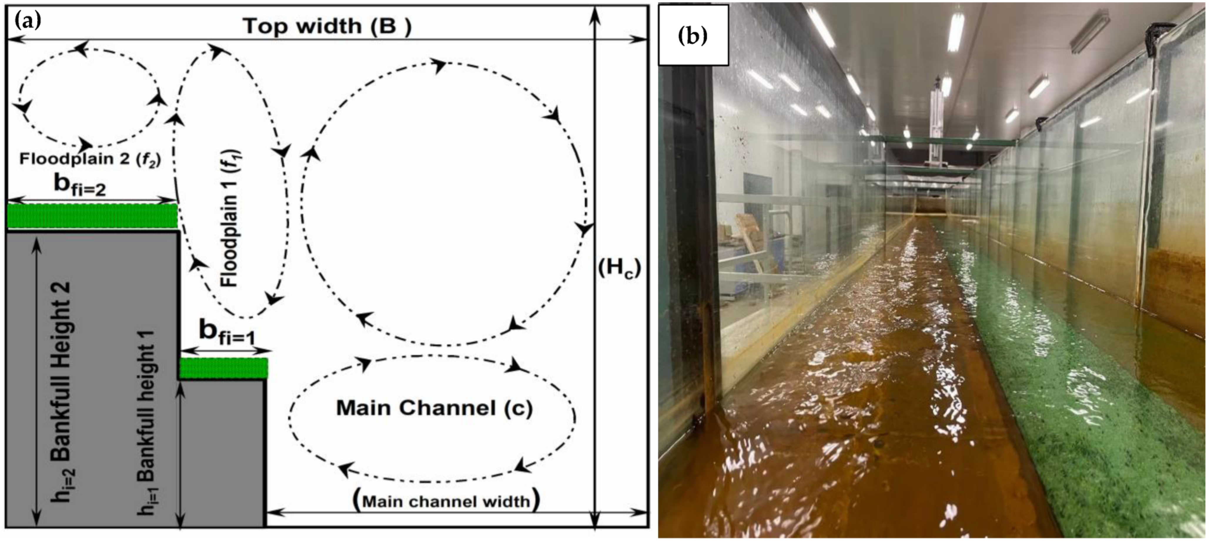
The present study focuses on the flow structure and interaction at the two interfaces of three flow zones with differential velocity in a multistage asymmetric channel, as shown in Figure 1a. The flow conditions for the experimental test case runs are chosen in such a way that it covers shallow flow (Dr < 0.3), intermediate flow (0.3 < Dr < 0.5) and high flow in (Dr > 0.5) conditions. Meanwhile, the numerical simulation objective is to explore the difference in the presence of the coherent structure across the two consequent staged interfaces with different bankfull heights. The turbulent structures over the staged floodplains of a compound open channel, including large-scale vortical structures and instantaneous secondary flows, are predicted, which plays a pivotal role in the flow resistance and sediment transport fluxes. The interaction of the main channel flow to the first and second-stage floodplain flow is discussed here. The overall study is arranged in the following order:
- The study’s experimental arrangements and flow setup are first described for the three test cases. The mathematical and numerical solution method is then discussed with a computational model setup.
- The validation of the experimental time-averaged primary mean velocity and secondary current are presented for three different depth ratios of multiple staged compound channels.
- Then, the streamwise primary velocity distribution, turbulence statistics and vortical structures to define the mass and momentum exchange are presented.
- The numerical model results and conclusions are made for the new flow configuration with staged floodplains.
Figure 1.
(a) Cross-sectional view of the staged floodplains and main channel of the experimental test case and (b) pictorial view from the downstream end of the compound channel with synthetic grass turf used for the floodplain. Note: denotes the flow depth in the main channel; is the top width; is the main channel width; and are floodplains’ depth and bed width, respectively.

2. Experimental Arrangements
The experiments were performed in a 20 m long and 0.745 m wide glassed-wall flume in the Fluid Mechanics Laboratory of Xi’an Jiaotong-Liverpool University (XJTLU), Suzhou, China. The multistage compound channel cross-section was rectangular, with a main channel width of 0.445 m, first-stage floodplain width of 0.1 m and second-stage floodplain width of 0.2 m (see Figure 1a). The floodplains were covered with flexible plastic grass turf, the density and blade height of which was 33,000 grass blades/cm2 and 8.3 mm, respectively (see Figure 1b). The bankfull height () of the first stage floodplain was 4 cm and the second stage floodplain had 8 cm, where or 2. With the dual existence of the interfacial section and bankfull height, the relative depth ratio was distinctively variable at each stage. The flow regime definition undertaken in this analysis is defined based on cm. However, it should be noted that for the first stage, the floodplain ( cm), was always a high-flow regime when . The measurement cross-section was located 11 m away from the flume inlet. An electromagnetic flowmeter was used to measure the upstream discharge. A honeycomb structure was installed in the stilling tank before the flume entrance to regulate the development and uniformity of the flow. The uniform section was maintained at all times by keeping the bed slope and the water surface slope equal through the downstream tailgate settings. The free water surface level was measured using a point gauge to obtain a free surface parallel to the channel bed.
In the Cartesian coordinate system, the instantaneous velocities, time-averaged velocities and velocity fluctuations are denoted as (,,), (,,) and (,,), respectively, in , and axes referring to the streamwise (along the flume), transverse and vertical (normal to the bed) directions. The flow condition is illustrated in Table 1. is evaluated from the log-law velocity distributions and averaged along the bed, where is the bed shear and is the density of water.
The velocity was measured using micro 3-D Nortek Vectrino side- and down-looking acoustic Doppler velocimetry (ADV), which has a sampling volume 5 cm away from the probe. At each measuring point, the three instantaneous velocity components (,,) were recorded at 200 Hz for 180–300 s (more time near the interface) with a signal-to-noise ratio greater than 18–20 and a no less than 75% correlation rate. The raw data from the ADV are despiked using the phase-space thresholding technique of Goring and Nikora [38]. The accuracy of the ADV was of the measured mean velocities. The maximum discrepancy between the discharge metered and the discharge obtained by velocity integration at the measurement cross-section was , the high value being associated with the second-stage floodplain at the lowest . The vertical (x-z) plane at the main channel and floodplain boundary is called the interface, and the position was denoted at ( cm and ( cm (refer to Figure 2a).
3. Numerical Model
Governing Equations
The incompressible Navier-Stokes equations were solved using the WMLES method, which can help to address the LES limitations for the high Reynolds number boundary layer using scale-resolving simulations [39]. WMLES helps to avoid high-resolution LES requirements near the wall region in wall-bounded scenarios, such as open channel flow. Shur et al. [40] proposed an approach for WMLES based on reformulating the length scale for the LES zone and blending it with the mixing length (RANS) model for the boundary layer zone.
where is the sub-grid scale turbulent viscosity, is the wall distance, is the strain rate, is the largest edge length of the current computational cell, is the cell size in wall direction, is used to define grid spacing and length of cell edges, ,, = 0.15 are some constants and is normal to the inner wall scaling. Using second-order accuracy, the following model was validated by the three flow depth data of the experimental test case in the staged compound channel. The basic LES methodology involves spatially filtering the vortices using the filter function. The small-scaled vortices are treated using the sub-grid scale stress (SGS) model, and the large-scale vortices are resolved using filtered incompressible Navier-Stokes equations (refer to Equations (3) and (4).
where represents the Cartesian coordinates (, corresponds to , and axes); and are the filtered velocity component; is the time; is the filtered pressure; =), the acceleration caused by gravity components, which are defined using bed slope. The term in Equation (4) for is the SGS stress tensor, which is resolved using Boussinesq’s hypothesis with being the strain rate tensor, is the sub-grid scale viscosity modelled using Equation (1), and based on the modified grid scale, WMLES models the wall-modelled flow based on grid anisotropy using Equation (2).
The computational model for the 20 m long experimental channel was set up using a 1 m scaled-down model of the channel using the periodic boundary for the inlet and outlet condition and the rigid lid assumption for the upper boundary. Many investigators have previously applied these assumptions for two-stage compound channels [41,42]. The computational domain of the , and cells gridded in the streamwise, transverse and vertical directions are created for three depth ratios, respectively. The near-wall modelling approach was employed for the bed and sidewalls of the open channel, in which the instantaneous shear stress was related to the velocity adjacent to the solid boundary using a time-averaged wall law. The rough height grass blade of the floodplain is given for the floodplain bed in the no-slip condition. The flow is driven by the gravity force identified by the component of in the streamwise direction. The initial conditions per periodic boundary conditions are the mass bulk flow velocity at the operating condition. After acquiring a statistical steady state, turbulence statistics were performed for 20 flow cycles of the ratio of the length of the modelled channel and bulk velocity.
This study discretises the governing equations using the finite volume method with advection terms discretised using high-resolution schemes [43,44] with higher-order accuracy and monotonicity. Meanwhile, the central difference scheme obtained a gradient of the pressure and diffusion terms. The SIMPLE algorithm was employed for the pressure-velocity coupling, and the second-order method was used for the transient flow.
4. Results and Discussion
The three-dimensional velocity components taken from ADV have been used to validate the main flow features. In particular, sampling standard errors for the critical parameters used in this study were estimated based on 30 time series, 3 min long, each at the same measuring point. These errors are found to be approximately 1.5% for the time-averaged velocities, i.e., (m/s). In this study, the ADV measurements very close to the free surface were not considered, especially for the z-components, as the ADV probe did not perform well in this region as the signal-to-noise ratio (SNR) was below the recommendations. The following section confirms the WMLES results for the streamwise velocity flow and secondary current for the three depth ratios of , and . Subsequently, the validation, instantaneous flow field, turbulence statistics and vortical structures are presented and analysed.
4.1. Distribution of the Mean Streamwise Velocity and Secondary Current
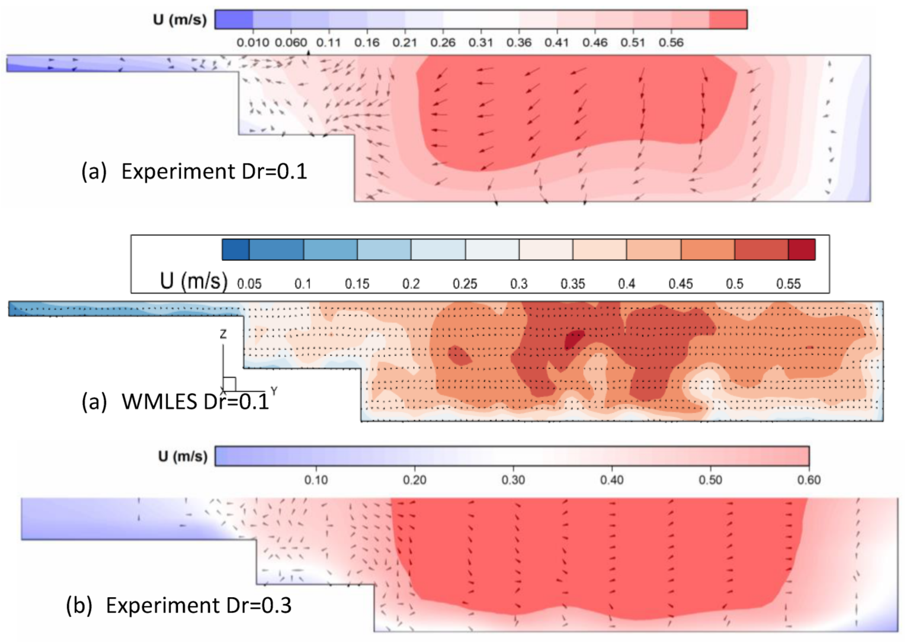
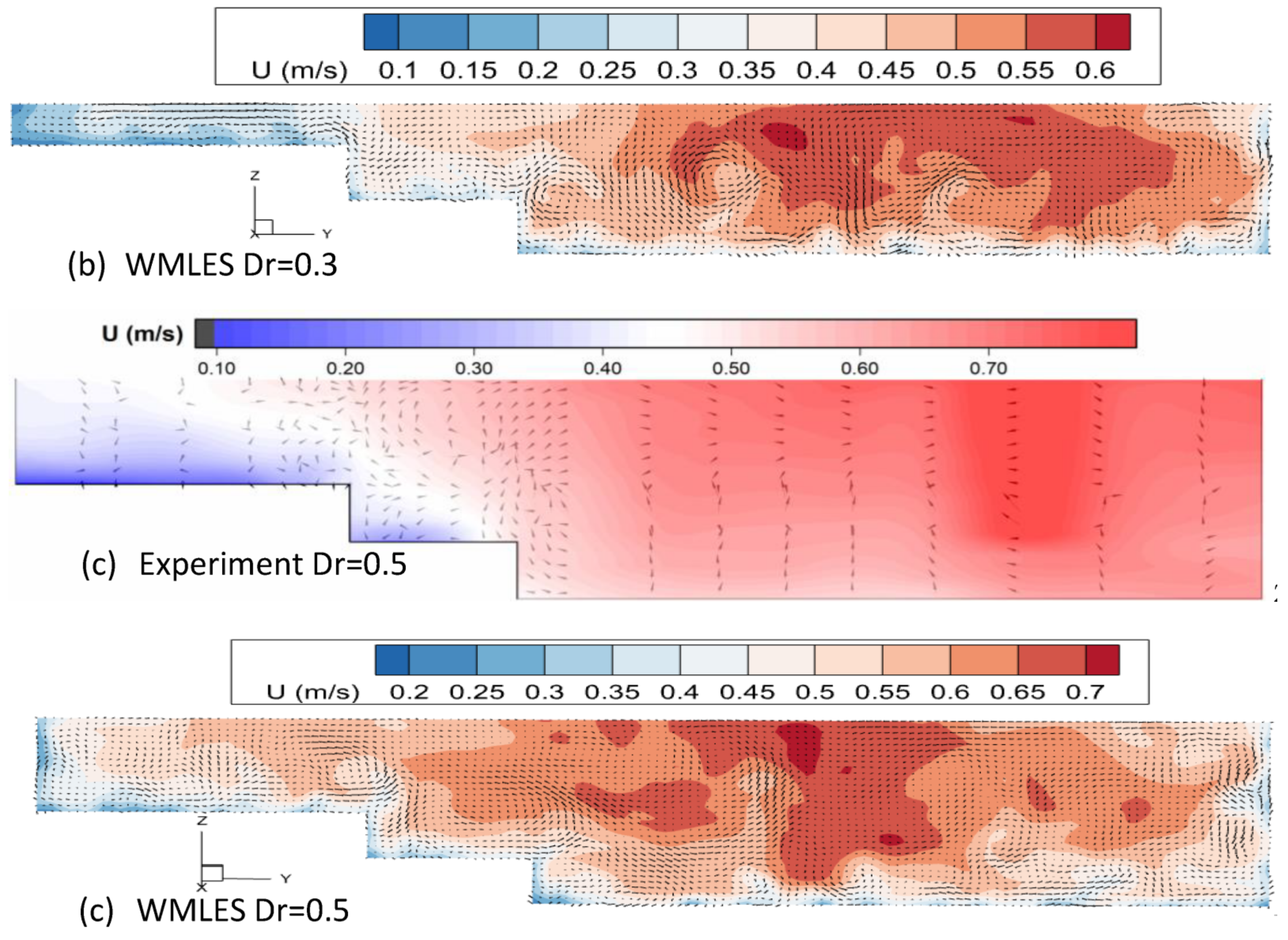
Figure 2 shows the cross-sectional distribution of the mean streamwise velocity () at three different flow depths () of 0.1, 0.3 and 0.5. The primary mean velocity is a crucial parameter linked to the compound open channel flow’s stage-discharge and flow resistance characteristics. The maximum velocity is located beneath the free surface at the main channel section (). For the lower flow depth (), the significant change in the mean velocity over the three stages of the compound section suggests a strong mixing layer, particularly between stage one () and stage two (). The velocity in this region of floodplain one is and in two,, the velocity is decelerated due to the low momentum transport caused by the secondary current.
The experimental measurements and the modelled results obtained using the WMLES model are shown in Figure 2 for comparison. The mean bulk velocity and the maximum velocity obtained from the present simulations are of the order of error, which has a reasonably close agreement with the measured experimental test runs. The main flow pattern of the interaction of the sub-section is depicted through the bulging of the primary velocity contours at the interface, which is well represented in Figure 2a–c for the WMLES results. This is outward bulging towards the free surface over the interface of the main channel, and floodplains one and two show an intense shearing due to the deceleration of the flow over the individual sections of flow. The interaction of the first floodplain and main channel significantly decelerates due to the low-speed flow transported by the secondary currents. The deceleration can be more feasibly observed near the free surface in the sidewall region and near the bottom of the main channel, which is well predicted in the WMLES model.
The vector description of the secondary current (longitudinal vortex) is shown for the experimental and numerical simulation, depicting strong inclined currents from the interface toward the free surface of the main channel to floodplains one and two. The horizontal flow from the side wall of the main channel towards the first floodplain (0.2 ≤ Y ≤ 0.3) is visible over the entire range of the depth ratio. There is even a clear free surface (Z ≥ 0.425) and bottom vortex at Z < 0.425 in the main channel for the higher Dr of the multistage channels. The detail of the secondary current is better depicted in the numerical results, which show the presence of different secondary cell generations at each consecutive stage of the asymmetric floodplains compared to the two-stage compound channels with a single floodplain.
4.2. Distribution of Instantaneous Streamwise Velocity
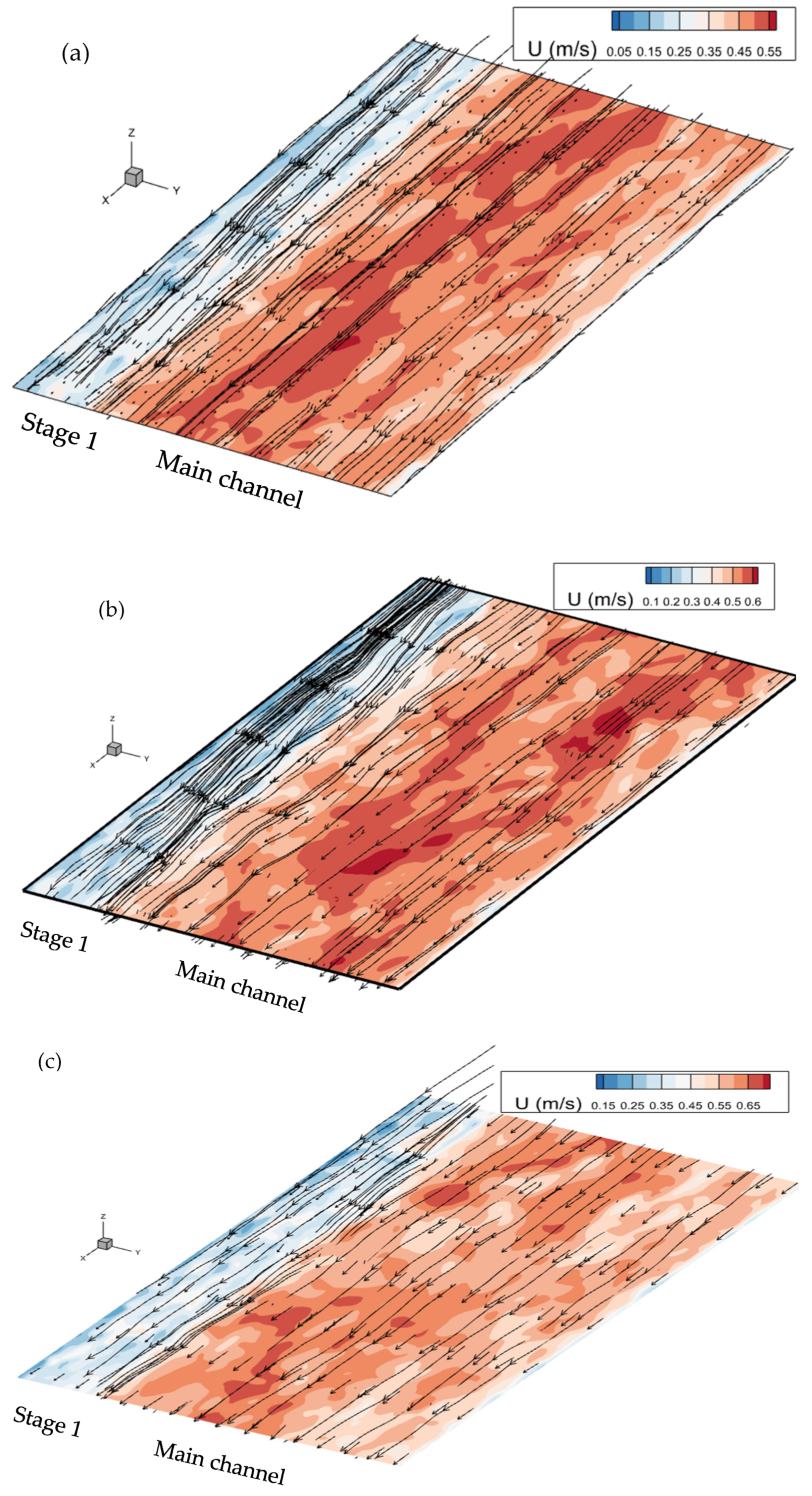
Figure 3 and Figure 4 show the snapshot of the distribution of the instantaneous velocity (), velocity vectors (,) and streamlines on a horizontal plane at the second ( m) and first ( m) bankfull height. Figure 3 illustrates the shear layer difference over the individual height of the banks for the multistage channel. The order of the velocity component in the streamwise direction increases with an increase in the depth ratio from to . Furthermore, as the streamwise velocity, u, is one order larger than the transverse velocity, in Figure 3 and Figure 4, the transverse velocity is increased by ten for clarity.
It is observed that the flow in the main channel is generally moving faster than in the first- and second-stage floodplains. Figure 3 shows a large shear region between the main channel and stages one and two. It is also evident that the effect of stage (floodplain) one subsides as the depth of flow increases above the intermediate zone (see Figure 3c). Furthermore, the junction of stage one shows a strong shearing, causing the mass and momentum transfer from the main channel to both floodplains. In Figure 4, a similar faster zone of the main channel section interacts with that of floodplain one. However, the bounded sidewall of floodplain one has a smaller velocity over the floodplain and, thus, becomes strongly advected by the streamwise flow of the main channel.
It is worth mentioning that although the instantaneous primary and secondary flows vary in space and time, demonstrating the complex three-dimensional turbulent flow structures, there is a slight variation for the time-averaged flow fields at different cross sections, and the main feature of compound open-channel flows can be recognised from the mean primary velocity and secondary currents (Figure 2).
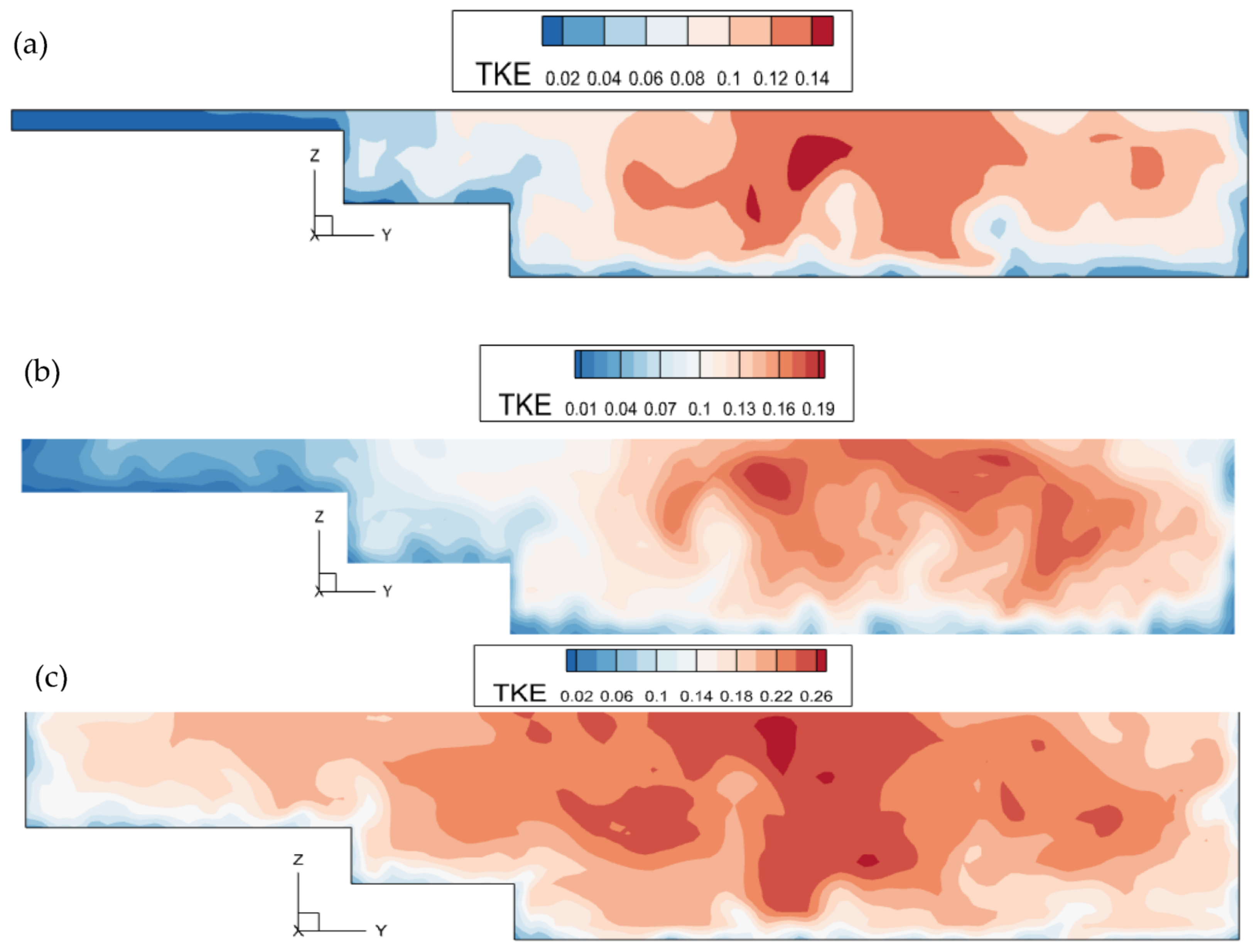
4.3. Distribution of Turbulent Kinetic Energy
Figure 5 shows the distribution of the turbulent kinetic energy (). The contour of the turbulent kinetic energy (TKE) shows a bulge at the interface of the main channel and floodplains one and two. This implies that the total magnitude of the turbulence increases near the interface edge. There is a high magnitude of turbulent energy near the middle region of the main channel towards floodplain one. The turbulent energy in the main channel section is higher, with a higher velocity gradient. The distribution of the TKE is similar to the pattern observed for the primary mean velocity. However, the bulge of TKE is not as strong as that of the primary mean velocity along the inclined up-flow.
4.4. Power Density Spectra (PSD) Using Time Series at Interfaces of Multistage Floodplains
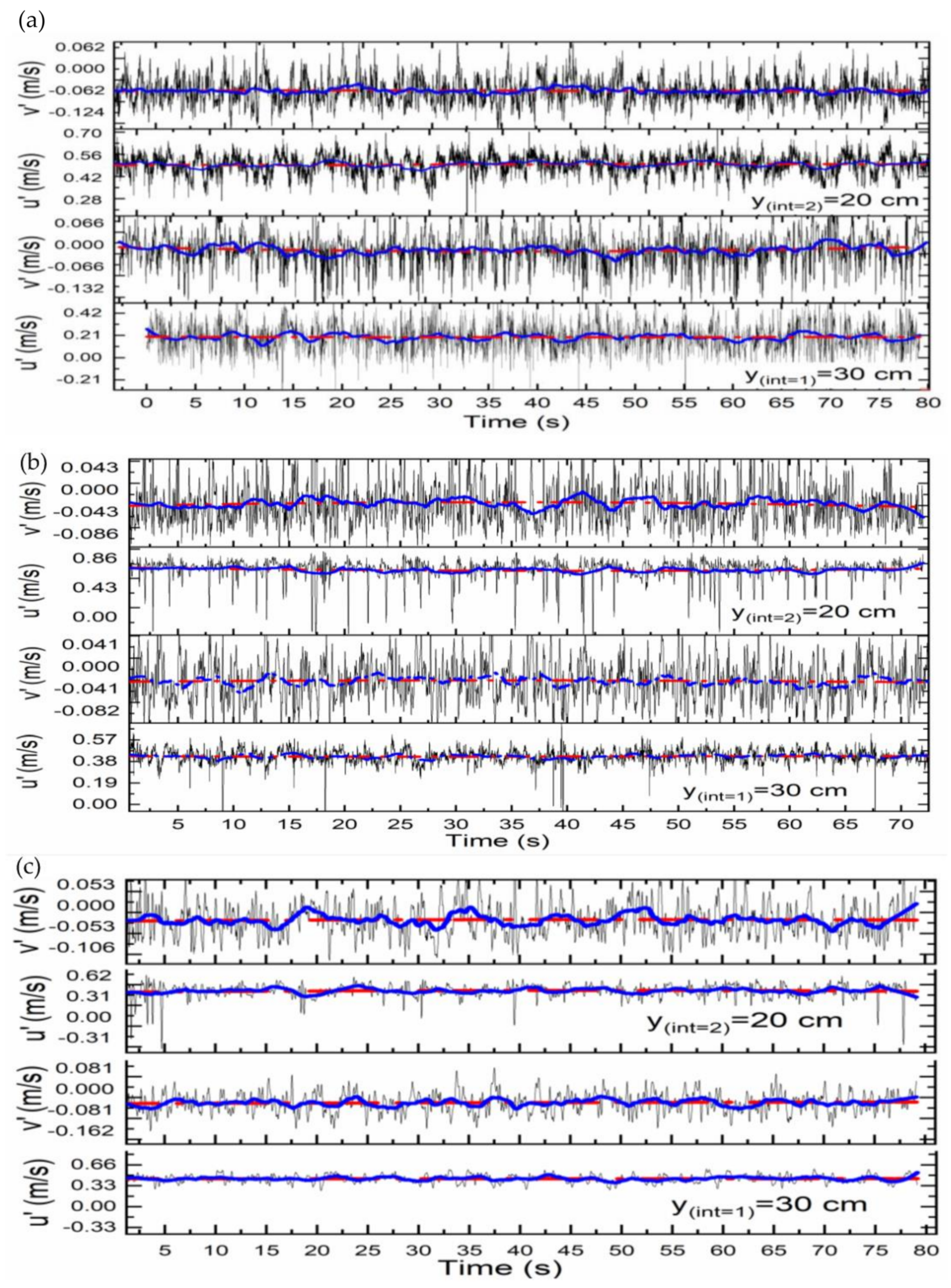
The time series of the streamwise and transverse velocities illustrates large quasi-periodic oscillations in the interface region, as shown in Figure 6 for the experimental test runs. These oscillations depict the formation of quasi-2D turbulence with 3D turbulence, which can be cross-verified with the spectral evolution in Figure 6a,b, characterising sharp bumps at a large scale. The interesting feature is that the low-pass filtered raw signals of and depicted in blue lines, have opposite phases (see Figure 6a–c). The consistency of the opposite phase of and can be seen in smaller depths, mainly corresponding to the interface cm, irrespective of the general depth ratio. These events of strong alternating phases induce coherent events, which persuade alternate successions of considerable sweeps (, ) at the interface cm and ejections (, ). Meanwhile, for the first interface cm, as the depth ratio tends towards , the coherent events subside in the mixing layer at a bankfull height of cm.
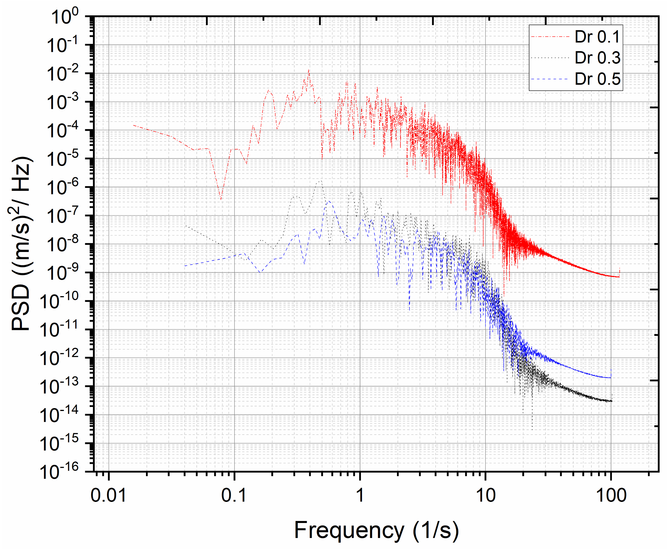
Figure 7 shows the power density spectra of the transverse velocity fluctuation for the three depth ratios, denoted as low (), intermediate () and high (), which were obtained numerically for the complete flow cycle over the turbulent statistics. The high-frequency side of all the peaks has a slope of approximately −5/3, indicating that the large turbulence structures possess 2D characteristics [45,46]. The peak in the PSD is attained at a comparatively higher frequency for the lower depth ratio (Figure 7). The appearance of a local peak within the intermediate frequency range always corresponds to the emergence of coherent structures. A noticeable range of a slope can be observed at the test cross-section, which depicts the well-developed coherent structures at all three depth ratios (Figure 8). Consequently, this results in high transverse turbulence intensities and Reynold shear stress values over all three depth ratios for the multistage compound open channels.
4.5. Vortical Structures
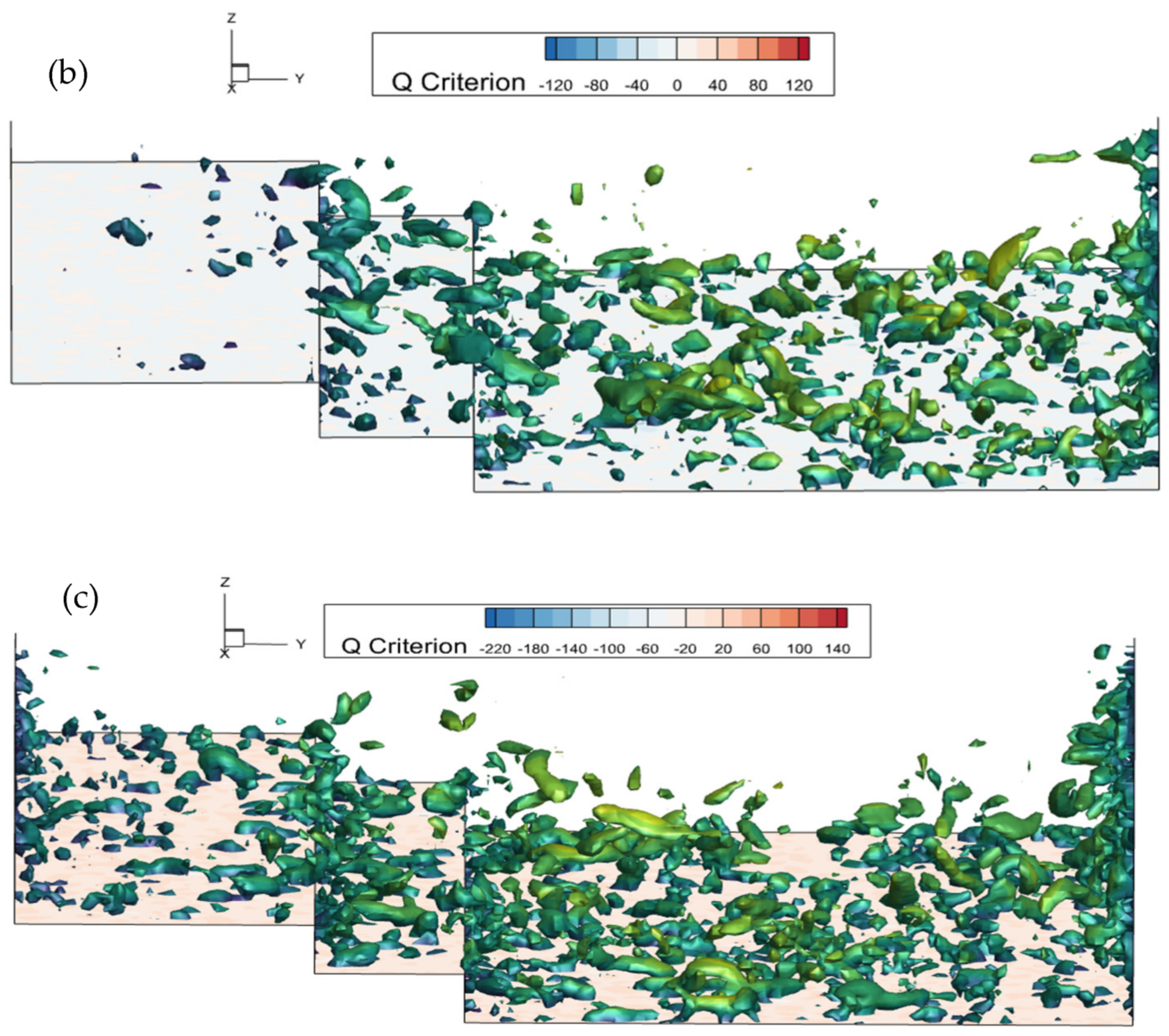
The Q-criterion is a method to define and identify the vortex structure in the turbulent flow [47], which is used here to analyse the instantaneous vertical structures of the multistage compound open channel for three depth ratios. Figure 8a–c shows the vertical structure from the shallow to deep flow regime in the staged floodplain one and two. The Q-value is defined through the gradient of the velocity components using the rotation rate tensor and the strain rate tensors.
It is seen from Figure 8 that when the depth of the flow increases, the vortex structures on the main channel and both floodplain stages gradually increase. Streamwise strip vortices are observed across the compound channel, with vortical structures concentrated near the bed and sidewalls showing high strain rates. One prominent visible feature is the elongated strip vortices advecting downstream of the compound channel. Furthermore, the location of the vortex cores varies in the streamwise direction, illustrating the chaotic flow field at the cross-section. The vortical structure near the sidewall of the main channel and at the interfaces, depicted through the strips of iso-surface, indicates a horizontal shear layer resulting from the horizontal Kelvin-Helmholtz (K-H) coherent structures. The K–H vortices enhanced the flow mixing in the horizontal direction. It is worth noting that the turbulence at the interface of stages one and two catapults with the increase in the flow depth.
5. Conclusions
Multistage compound channels with rough floodplains covered with grass turf roughness were experimentally investigated. Different depth ratios were tested with a uniform steady-state condition, where the turbulent exchange process was investigated experimentally and analytically using ADV to understand the flow mechanism in these new configurations. The distribution of the primary mean velocity and secondary currents is validated using WMLES for three depth ratios of the multistage compound open channel. The turbulent kinetic energy, instantaneous vortical structure and coherent structure generation for the different cases illustrate the mass transfer mechanism under staged floodplains. The main source of turbulence in the channel is shearing, which creates a region of high lateral turbulence statistics around the interface of the second-stage floodplains. Another source of turbulence is the boundary layer based on the bottom and sidewalls of the main channel, and this turbulence diffuses towards the free surface. The instantaneous flow fields and large-scale vortical structures are presented, which show a strong turbulent flow near the sidewall and the interfaces of the multistage compound channel. Lastly, the WMLES demonstrates the capability to provide reliable mean velocity fields for the staged floodplains of the compound open channel. This study’s future perspective would include macro-roughness over the higher stage of floodplains to investigate the flow resistance and mass exchange.
The study demonstrates the capability of the present WMLES model to provide reliable, detailed mean velocity field characteristics and turbulence statistics for multiple staged open-channel flows, which can act as a complementary approach to experimental investigations to gain further insight into the turbulent flow dynamics. The main future extension of this study would be to include a solute transport module and roughness effect to investigate the mass exchange between the main channel and the floodplains.
Author Contributions
P.K.S.: Conceptualization, Investigation, Methodology, Formal analysis, Writing—original draft, data curation, validation; X.T.: Conceptualization, Methodology, supervision, writing—review and editing; H.R.: writing—review and editing. All authors have read and agreed to the published version of the manuscript.
Funding
This research was funded by the National Natural Science Foundation of China (11772270).
Institutional Review Board Statement
Not applicable.
Informed Consent Statement
Not applicable.
Data Availability Statement
There are no new data created.
Acknowledgments
The authors would like to acknowledge the National Natural Science Foundation of China (11772270) and the funding of XJTLU (KSF-E-17, RDF-16-02-02). Furthermore, the authors would also like to sincerely thank all the past researchers who gave valuable experimental datasets.
Conflicts of Interest
The authors declare that they have no known competing financial interests or personal relationships that could have influenced the work reported in this paper.
References
- Abril, J.; Knight, D. Stage-discharge prediction for rivers in flood applying a depth-averaged model. J. Hydraul. Res. 2004, 42, 616–629. [Google Scholar] [CrossRef]
- Knight, D. Hydraulic problems in flooding: From data to theory and from theory to practice. In Experimental and Computational Solutions of Hydraulic Problems; Springer: Berlin/Heidelberg, Germany, 2013; pp. 19–52. [Google Scholar]
- Cappato, A.; Baker, E.A.; Reali, A.; Todeschini, S.; Manenti, S. The role of modeling scheme and model input factors uncertainty in the analysis and mitigation of backwater induced urban flood-risk. J. Hydrol. 2022, 614, 128545. [Google Scholar] [CrossRef]
- Knight, D.W.; Shiono, K. Turbulence measurements in a shear layer region of a compound channel. J. Hydraul. Res. 1990, 28, 175–196. [Google Scholar] [CrossRef]
- Peltier, Y. Physical Modelling of Overbank Flows with a Groyne Set on the Floodplain. Ph.D. Thesis, Université Claude Bernard-Lyon I, Lyon, France, 2011. [Google Scholar]
- Atabay, S. Stage-Discharge, Resistance, and Sediment Transport Relationships for Flow in Straight Compound Channels. Doctoral Dissertation, University of Birmingham, Birmingham, UK, 2001. Available online: https://ethos.bl.uk/OrderDetails.do?uin=uk.bl.ethos.427466 (accessed on 14 February 2023).
- Knight, D.W.; Demetriou, J.D. Flood Plain and Main Channel Flow Interaction. J. Hydraul. Eng. 1983, 109, 1073–1092. [Google Scholar] [CrossRef]
- Singh, P.; Tang, X. Interfacial compound section transverse flow variation in symmetric and asymmetric compound open channel flow. In Proceedings of the 9th International Symposium on Environmental Hydraulics, Seoul, Republic of Korea, 18–22 July 2021; pp. 174–175. [Google Scholar]
- Singh, P.; Tang, X.; Rahimi, H.R. Modelling of the apparent shear stress for predicting zonal discharge in rough and smooth asymmetric compound open channels. In River Flow 2020: Proceedings of the 10th Conference on Fluvial Hydraulics, Delft, The Netherlands, 7–10 July 2020; CRC Press/Balkema (Taylor & Francis): Leiden, The Netherlands, 2020; pp. 84–94. [Google Scholar]
- Nicollet, G.; Uan, M. Ecoulements permanents à surface libre en lits composes. La Houille Blanche 1979, 21–30. [Google Scholar] [CrossRef] [Green Version]
- Knight, D.W.; Hamed, M.E. Boundary Shear in Symmetrical Compound Channels. J. Hydraul. Eng. 1984, 110, 1412–1430. [Google Scholar] [CrossRef]
- Tominaga, A.; Nezu, I. Turbulent Structure in Compound Open-Channel Flows. J. Hydraul. Eng. 1991, 117, 21–41. [Google Scholar] [CrossRef]
- Fernandes, J. Compound channel uniform and non-uniform flows with and without vegetation in the floodplain. Ph.D. Thesis, Departamento de Engenharia Civil, Instituto Superior Técnico da Universidade Técnica de Lisboa, Lisboa, Portugal, 2013. [Google Scholar]
- Tang, X.; Knight, D.W. Sediment Transport in River Models with Overbank Flows. J. Hydraul. Eng. 2006, 132, 77–86. [Google Scholar] [CrossRef]
- Pasche, E.; Rouvé, G. Overbank flow with vegetatively roughened flood plains. J. Hydraul. Eng. 1985, 111, 1262–1278. [Google Scholar] [CrossRef]
- Kozioł, A.P. Three-Dimensional Turbulence Intensity in a Compound Channel. J. Hydraul. Eng. 2013, 139, 852–864. [Google Scholar] [CrossRef]
- Dupuis, V.; Proust, S.; Berni, C.; Paquier, A. Mixing layer development in compound channel flows with submerged and emergent rigid vegetation over the floodplains. Exp. Fluids 2017, 58, 1–18. [Google Scholar] [CrossRef] [Green Version]
- Tang, X.; Rahimi, H.R.; Wang, Y.U.; Zhao, Y.U.; Lu, Q.I.; Wei, Z.I.; Singh, P.R. Flow characteristics of open-channel flow with partial two-layered vegetation. In Proceedings of the 38th IAHR World Congress, Panama City, Panama, 1–6 September 2019; pp. 1–6. [Google Scholar]
- Tang, X.; Guan, Y.; Rahimi, H.; Singh, P.; Zhang, Y. Discharge and velocity variation of flows in open channels partially covered with different layered vegetation. E3S Web Conf. 2021, 269, 03001. [Google Scholar] [CrossRef]
- Proust, S.; Fernandes, J.N.; Leal, J.B.; Rivière, N.; Peltier, Y. Mixing layer and coherent structures in compound channel flows: Effects of transverse flow, velocity ratio, and vertical confinement. Water Resour. Res. 2017, 53, 3387–3406. [Google Scholar] [CrossRef]
- Proust, S.; Fernandes, J.N.; Peltier, Y.; Leal, J.B.; Riviere, N.; Cardoso, A.H. Turbulent non-uniform flows in straight compound open-channels. J. Hydraul. Res. 2013, 51, 656–667. [Google Scholar] [CrossRef] [Green Version]
- Naik, B.; Khatua, K.K.; Padhi, E.; Singh, P. Loss of Energy in the Converging Compound Open Channels. Arab. J. Sci. Eng. 2017, 43, 5119–5127. [Google Scholar] [CrossRef]
- Rajaratnam, N.; Ahmadi, R. Hydraulics of channels with floodplains. J. Hydraul. Res. 1981, 19, 43–60. [Google Scholar] [CrossRef]
- Kara, S.; Stoesser, T.; Sturm, T.W. Turbulence statistics in compound channels with deep and shallow overbank flows. J. Hydraul. Res. 2012, 50, 482–493. [Google Scholar] [CrossRef]
- Naot, D.; Nezu, I.; Nakagawa, H. Hydrodynamic Behavior of Compound Rectangular Open Channels. J. Hydraul. Eng. 1993, 119, 390–408. [Google Scholar] [CrossRef]
- Lin, B.; Shiono, K. Numerical modelling of solute transport in compound channel flows. J. Hydraul. Res. 1995, 33, 773–788. [Google Scholar] [CrossRef]
- Sofialidis, D.; Prinos, P. Numerical Study of Momentum Exchange in Compound Open Channel Flow. J. Hydraul. Eng. 1999, 125, 152–165. [Google Scholar] [CrossRef]
- Cokljat, D.; Younis, B.A. Second-Order Closure Study of Open-Channel Flows. J. Hydraul. Eng. 1995, 121, 94–107. [Google Scholar] [CrossRef]
- Kang, H.; Choi, S.-U. Turbulence modeling of compound open-channel flows with and without vegetation on the floodplain using the Reynolds stress model. Adv. Water Resour. 2006, 29, 1650–1664. [Google Scholar] [CrossRef]
- Jing, H.; Li, C.; Guo, Y.; Xu, W. Numerical simulation of turbulent flows in trapezoidal meandering compound open channels. Int. J. Numer. Methods Fluids 2011, 65, 1071–1083. [Google Scholar] [CrossRef]
- Singh, P.K.; Tang, X.; Rahimi, H. A Computational Study of Interaction of Main Channel and Floodplain: Open Channel Flows. J. Appl. Math. Phys. 2020, 08, 2526–2539. [Google Scholar] [CrossRef]
- Wang, W.; Huai, W.-X.; Gao, M. Numerical investigation of flow through vegetated multi-stage compound channel. J. Hydrodyn. 2014, 26, 467–473. [Google Scholar] [CrossRef]
- Chen, G.; Zhao, S.; Huai, W.; Gu, S. General model for stage–discharge prediction in multi-stage compound channels. J. Hydraul. Res. 2018, 57, 517–533. [Google Scholar] [CrossRef]
- Menter, F.; Schutze, J.; Kurbatskii, K.; Lechner, R.; Gritskevich, M.; Garbaruk, A. Scale-Resolving simulation techniques in industrial CFD. In Proceedings of the 6th AIAA Theoretical Fluid Mechanics Conference, Honolulu, HI, USA, 27–30 June 2011; p. 3474. [Google Scholar]
- Thomas, T.; Williams, J. Large eddy simulation of turbulent flow in an asymmetric compound open channel. J. Hydraul. Res. 1995, 33, 27–41. [Google Scholar] [CrossRef]
- Cater, J.E.; Williams, J.J.R. Large eddy simulation of a long asymmetric compound open channel. J. Hydraul. Res. 2008, 46, 445–453. [Google Scholar] [CrossRef]
- Xie, Z.; Lin, B.; Falconer, R.A. Large-eddy simulation of the turbulent structure in compound open-channel flows. Adv. Water Resour. 2012, 53, 66–75. [Google Scholar] [CrossRef]
- Goring, D.G.; Nikora, V.I. Despiking acoustic Doppler velocimeter data. J. Hydraul. Eng. 2002, 128, 117–126. [Google Scholar] [CrossRef] [Green Version]
- Nikitin, N.V.; Nicoud, F.; Wasistho, B.; Squires, K.; Spalart, P.R. An approach to wall modeling in large-eddy simulations. Phys. Fluids 2000, 12, 1629–1632. [Google Scholar] [CrossRef]
- Shur, M.L.; Spalart, P.R.; Strelets, M.K.; Travin, A.K. A hybrid RANS-LES approach with delayed-DES and wall-modelled LES capabilities. Int. J. Heat Fluid Flow 2008, 29, 1638–1649. [Google Scholar] [CrossRef]
- Zeng, C.; Bai, Y.; Zhou, J.; Qiu, F.; Ding, S.; Hu, Y.; Wang, L. Large Eddy Simulation of Compound Open Channel Flows with Floodplain Vegetation. Water 2022, 14, 3951. [Google Scholar] [CrossRef]
- Ding, S.-W.; Zeng, C.; Zhou, J.; Wang, L.-L.; Chen, C. Impact of depth ratio on flow structure and turbulence characteristics of compound open channel flows. Water Sci. Eng. 2021, 15, 265–272. [Google Scholar] [CrossRef]
- Hussaini, M.Y.; Zang, T.A. Spectral methods in fluid dynamics. Annu. Rev. Fluid 1987, 19, 339–367. [Google Scholar] [CrossRef]
- Hirsch, C. Numerical Computation of Internal and External Flows: The Fundamentals of Computational Fluid Dynamics; Elsevier: Amsterdam, The Netherlands, 2007. [Google Scholar]
- Uijttewaal, W.S.J.; Booij, R. Effects of shallowness on the development of free-surface mixing layers. Phys. Fluids 2000, 12, 392–402. [Google Scholar] [CrossRef]
- Batchelor, G.K. Computation of the Energy Spectrum in Homogeneous Two-Dimensional Turbulence. Phys. Fluids 1969, 12, II-233–II-239. [Google Scholar] [CrossRef]
- Hunt, J.C.; Wray, A.A.; Moin, P. Eddies, streams, and convergence zones in turbulent flows. In Studying Turbulence Using Numerical Simulation Databases, 2. Proceedings of the 1988 Summer Program; NASA: Washington, DC, USA, 1988; p. 19890015184142023. Available online: https://ntrs.nasa.gov/citations/19890015184 (accessed on 14 February 2023).
Figure 2.
Contour mapping of the streamwise mean velocity for experimental and numerical results for three depth ratios as (a) Dr = 0.1, (b) Dr = 0.3 and (c) Dr = 0.5.
Figure 2.
Contour mapping of the streamwise mean velocity for experimental and numerical results for three depth ratios as (a) Dr = 0.1, (b) Dr = 0.3 and (c) Dr = 0.5.


Figure 3.
The distribution of the instantaneous streamwise velocity and the velocity vectors (, ) for (a) , (b) and (c) to illustrate the shear layer at a horizontal plane at second stage , for a constant time interval of times of flow cycle. The values of are increased by a factor of 10 for clarity.

Figure 4.
The distribution of the instantaneous streamwise velocity u and the velocity vectors (u, w) for (a) Dr = 0.1, (b) Dr = 0.3 and (c) Dr = 0.5 to illustrate the shear layer at a horizontal plane at the first stage Z = 0.04 m, for a constant time interval of 0.1 times of flow cycle. A factor of 10 for clarity increases the values of w.

Figure 5.
Contour mapping of the turbulent kinetic energy in m2/s2 for (a) Dr = 0.1, (b) Dr = 0.3 and (c) Dr = 0.5.
Figure 5.
Contour mapping of the turbulent kinetic energy in m2/s2 for (a) Dr = 0.1, (b) Dr = 0.3 and (c) Dr = 0.5.

Figure 6.
Time series of streamwise () and lateral velocities () for depth ratio (Dr) being (a) 0.1, (b) 0.3 and (c) 0.5 at the interface of cm with h = 0.85 cm and cm with h = 0.45 cm. The black line is the raw signal, the blue line is the low-pass filtered signal and the solid red line is the mean value of the raw signal.

Figure 7.
Power spectral density (PSD) of transverse velocity fluctuations v′, as a function of frequency for the three depth ratios.
Figure 7.
Power spectral density (PSD) of transverse velocity fluctuations v′, as a function of frequency for the three depth ratios.

Figure 8.
Instantaneous vortical structure plotted as iso-surfaces of for Dr at (a) 0.1, (b) 0.3 and (c) 0.5, respectively, and coloured by the x-velocity component in the multistage compound open-channel flows.
Figure 8.
Instantaneous vortical structure plotted as iso-surfaces of for Dr at (a) 0.1, (b) 0.3 and (c) 0.5, respectively, and coloured by the x-velocity component in the multistage compound open-channel flows.


Table 1.
Flow conditions of test cases. Note that is the total discharge and denotes the Reynolds number.
Table 1.
Flow conditions of test cases. Note that is the total discharge and denotes the Reynolds number.
| 0.1 | 0.0910 | 0.02536 | 1.27 | 9.44 | 0.86 |
| 0.3 | 0.1108 | 0.03542 | 1.46 | 7.40 | 1.36 |
| 0.5 | 0.1617 | 0.06075 | 1.76 | 7.62 | 2.39 |
Disclaimer/Publisher’s Note: The statements, opinions and data contained in all publications are solely those of the individual author(s) and contributor(s) and not of MDPI and/or the editor(s). MDPI and/or the editor(s) disclaim responsibility for any injury to people or property resulting from any ideas, methods, instructions or products referred to in the content. |
© 2023 by the authors. Licensee MDPI, Basel, Switzerland. This article is an open access article distributed under the terms and conditions of the Creative Commons Attribution (CC BY) license (https://creativecommons.org/licenses/by/4.0/).
Share and Cite
MDPI and ACS Style
Singh, P.K.; Tang, X.; Rahimi, H. Large-Eddy Simulation of Compound Channels with Staged Floodplains: Flow Interactions and Turbulent Structures. Water 2023, 15, 983. https://doi.org/10.3390/w15050983
AMA Style
Singh PK, Tang X, Rahimi H. Large-Eddy Simulation of Compound Channels with Staged Floodplains: Flow Interactions and Turbulent Structures. Water. 2023; 15(5):983. https://doi.org/10.3390/w15050983
Chicago/Turabian StyleSingh, Prateek Kumar, Xiaonan Tang, and Hamidreza Rahimi. 2023. "Large-Eddy Simulation of Compound Channels with Staged Floodplains: Flow Interactions and Turbulent Structures" Water 15, no. 5: 983. https://doi.org/10.3390/w15050983
Note that from the first issue of 2016, this journal uses article numbers instead of page numbers. See further details here.