Optimizing Low Impact Development for Stormwater Runoff Treatment: A Case Study in Yixing, China

Abstract

Low-impact development (LID) practices have been recognized as a promising strategy to control urban stormwater runoff and non-point source pollution in urban ecosystems. However, many experimental and modeling efforts are required to tailor an effective LID practice based on the hydraulic and environmental characteristics of a given region. In this study, the InfoWorks ICM was applied to simulate the runoff properties and determine the optimal LID design in a residential site at Yixing, China, based on four practical rainfall events. Additionally, the software was redeveloped using Ruby object-oriented programming to improve its efficiency in uncertainty analysis using the Generalized Likelihood Uncertainty Estimation method. The simulated runoff was in good agreement with the observed discharge (Nash–Sutcliffe model efficiency coefficients >0.86). The results of the response surface method indicated that when the sunken green belt, permeable pavement, and green roof covered 8.6%, 15%, and 10%, respectively, of the 11.3 ha study area, the designed system showed the best performance with relatively low cost. This study would provide new insights into designing urban rainfall-runoff pollution control systems.

1. Introduction

Urbanization, characterized by continuous growth in population and land development, has altered the urban water cycle. Increasing urban impervious areas disrupted the infiltration process and resulted in a significant increase in the amount of surface water runoff, intensifying the frequency and severity of floods [1,2,3]. Besides, the growing population and industry largely augment the pollution load, such as through emissions from vehicles, the use of pharmaceuticals and personal care products, and the release of micro-/nano-plastics [4,5,6]. These pollutants exhibit stronger interactions with each other and may enrich adverse substances such as antibiotic resistance genes in surface water and floods [7,8]. One of the greatest issues in urban runoff is the first flush effect (FFE), which implies a greater discharge rate of pollutant mass or concentration in the early part of the runoff as compared with later in the storm [9,10,11]. Chow and Yusop (2014) [9] examined the water quality of 52 rainfall events and concluded that the first 10 mm of rainfall carried about 50% of the total pollutants. Wang et al. (2016) [10] proposed that intercepting the first 30–40% of the surface runoff was the most effective in stormwater quality management. As a result, controlling the first flush is critical for stormwater management.

Low impact development (LID) has been regarded as a promising strategy to compensate for the influence of urbanization on hydrology and water quality by simulating the pre-development site hydrology with site design techniques [12,13]. LID, as an effective and environmentally friendly practice for urban runoff management, is capable of significantly reducing urban runoff pollution loads [14]. This strategy was first introduced by the U.S. Environmental Protection Agency in the 1990s and has been widely used in many cities [12,15,16]. Green infrastructures such as bioretention cells, green roofs, and permeable pavements are implemented for LID purposes [17,18]. However, the design and implementation of these green infrastructures require optimization to achieve better performance [14,19].

Due to the random and uneven distribution of surface runoff, optimizing LID practices based on model simulation has become an ideal strategy. SWMM, MIKE, and InfoWorks ICM were often used by researchers to simulate the quality and quantity of surface runoff [20,21,22]. SWMM is a commonly used software that is easy to operate and commonly applied for secondary development. However, its input was complicated, and the results were difficult to visualize [20,22]. MIKE was feasible to simulate the hydraulics and quality, but some models required to be coupled manually [21]. InfoWorks ICM, developed by Wallingford, facilitated the operation and visualization of the urban water cycle simulation, making it a preferable choice for this study [23,24]. For example, Fan et al. (2022) [25] applied InfoWorks ICM to analyze the hydrological and pollution reduction in outfall and storage under different hydrological patterns, vertical parameter settings, and green infrastructure installation locations. However, most of the stormwater management practices in China only focused on reducing the volume rather than the FFE, which is key to a more effective LID practice design and stormwater runoff management [23,26].

Therefore, the aims of this study are: (1) to establish a model using InfoWorks ICM for stormwater runoff quality monitoring and estimation; (2) to conduct sensitivity analysis, calibration, validation, and uncertainty analysis on the established model; and (3) to optimize various LID facilities to maximize their performance while minimizing the cost. This study presents a promising method for urban runoff management, and the results are available for decision-makers to use in future planning.

2. Materials and Methods

2.1. Site Description

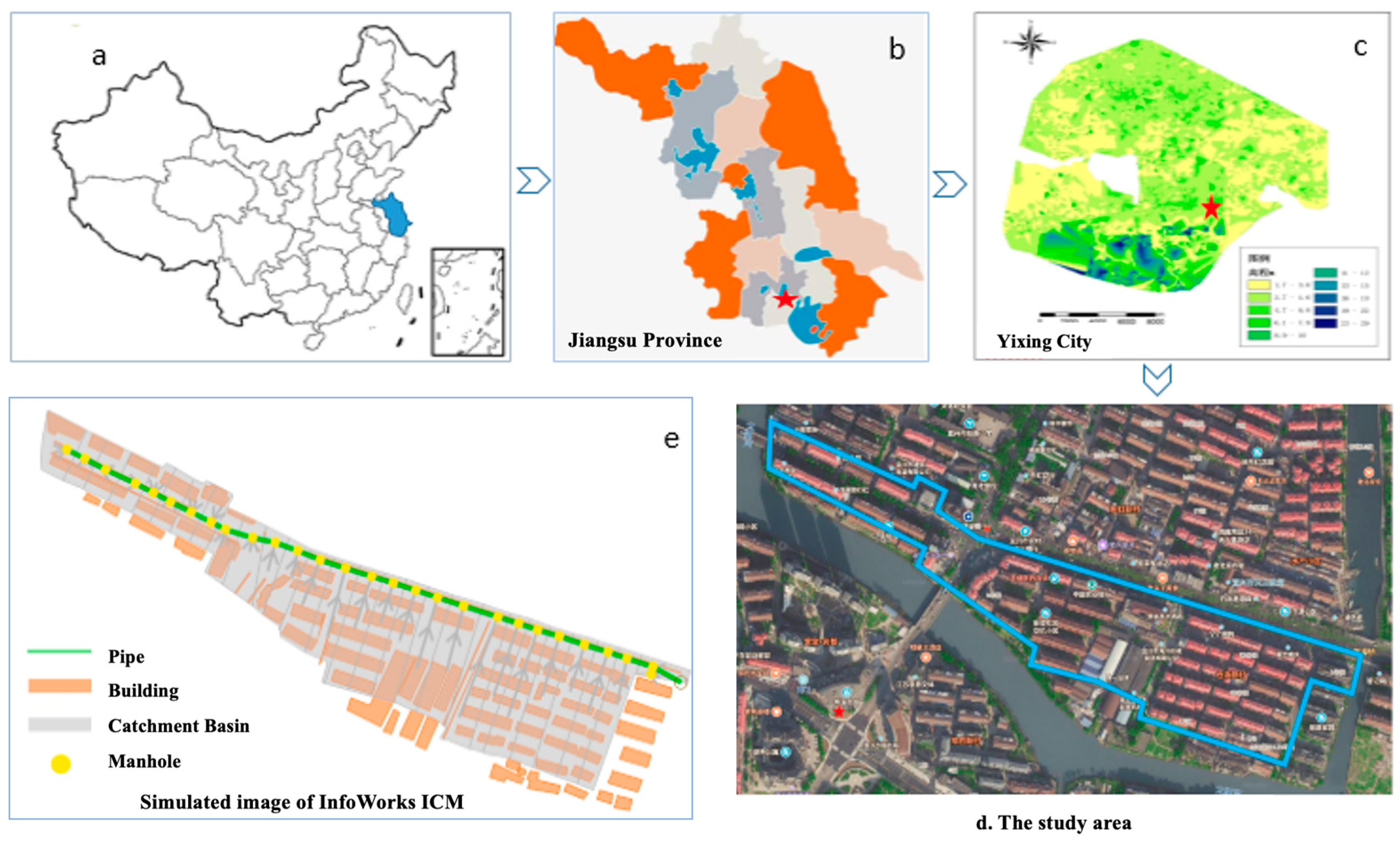
This study took place in Yixing (31°07′~31°37′ N, 119°31′~120°03′ E), a city located in the Southern part of Jiangsu Province, China (Figure 1). Yixing is hilly in the south, flat in the north, and has Taihu Lake to the east. The city has a humid subtropical climate and is influenced by the East Asian monsoon, which results in four distinct seasons and dense river networks. The average annual rainfall is 1177 mm and mostly occurs during the spring and summer. Rapid urbanization results in a growing amount of waste and poses a threat to the environment, especially the Taihu Lake. Therefore, the control and management of non-point pollution are of great significance. The study was conducted in a 0.1113 km² residential area with 8.6% green area, 48.4% construction area, and the remaining 43% roads.

2.2. Stormwater Sampling and Data Acquisition

Flowrates were monitored at 5–10 min intervals, and the samples for water quality analysis were manually collected in 500 mL polyethylene bottles. The data for four rainfall events (7 November 2015, 22 August 2015, 5 April 2018, and 23 April 2018) were acquired from the automatic rain gages at the 104 freeway, which recorded every 0.2 mm.

Then, the collected samples were sent to the laboratory for water quality analysis. The samples were kept in the fridge before analysis, and all the experiments were performed within 24 h. The concentrations of suspended solids (SS), NH₄⁺-N, chemical oxygen demand (COD), and total phosphorus (TP) were measured by the weighing method, Nessler’s reagent spectrophotometry method, rapid digestion spectrophotometry method, and Mo-Sb anti-spectrophotometric method, respectively.

2.3. Data from Stormwater Monitoring

Four different storm events were used to calibrate and validate the rainfall-runoff model (

Table 1. Data from stormwater monitoring.

	Previous Dry Duration (h)	Depth (mm)	Duration (min)	Average Intensity (mm/h)	Characterization
22 August 2015	39	20.2	420	2.89	Moderate
11 July 2015	18	13.0	150	5.20	Heavy
4 May 2018	22	9.0	160	3.38	Moderate
23 April 2018	3	55.0	576	5.73	Heavy

): storm events on 22 August 2015 and 11 July 2015 for the calibration process and storm events on 4 May 2018 and 23 April 2018 for validation.

2.4. Rainfall-Runoff Pollution Model Setup

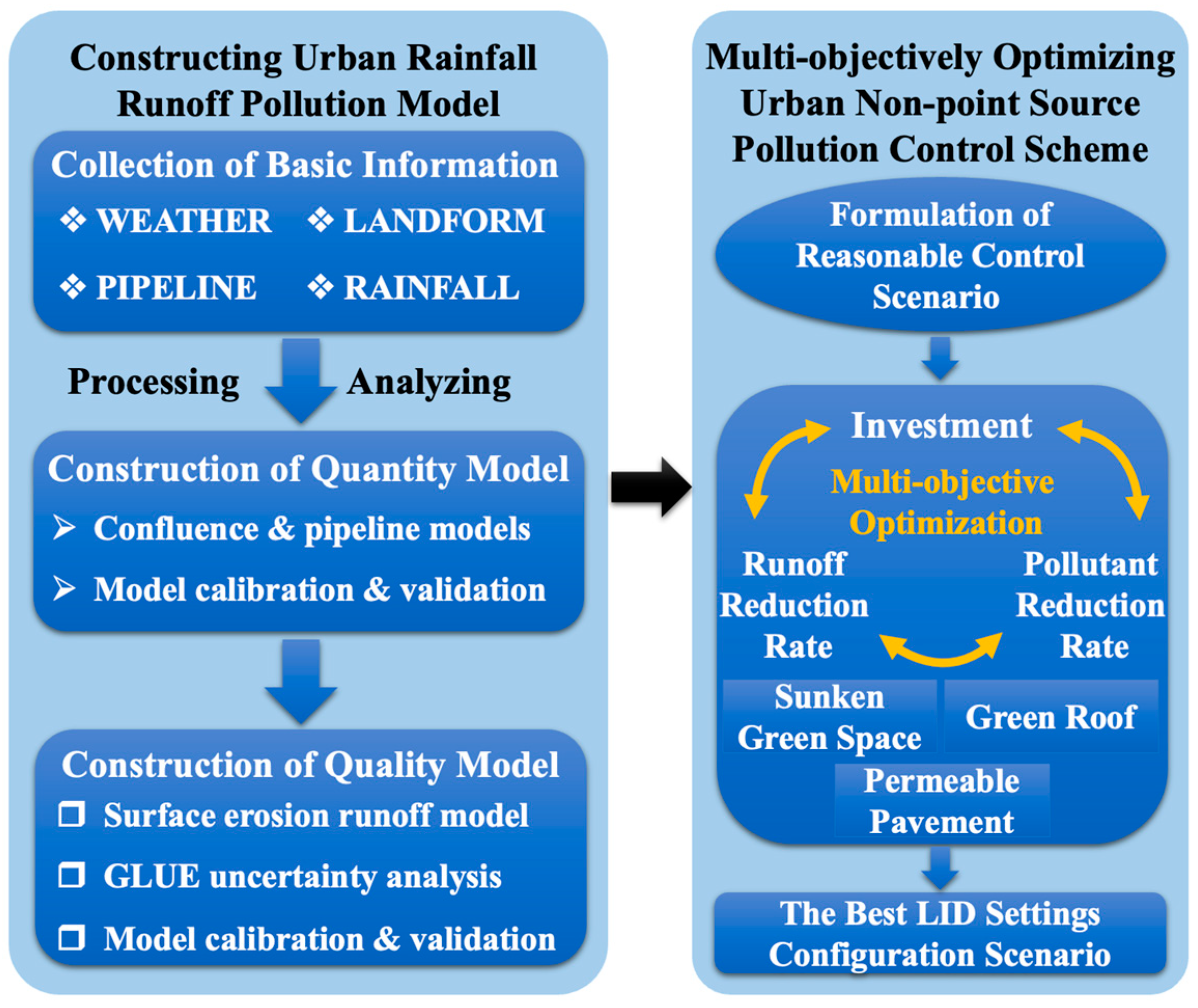
InfoWorks ICM was applied to set up an urban rainfall-runoff pollution model, including a hydrologic module and a water quality module (Figure 2). In the hydrologic module, the surface runoff in impervious areas, including roads and buildings, was calculated by the rational method, while the infiltration in the green areas was estimated using the Horton equation [26,27]. The nonlinear reservoir method was applied in the routing model. Since the study area has a separate sewer system, only the storm drain was simulated using the Saint-Venant equations. In the model, the pipelines were generalized into connecting lines between nodes, and the boundary conditions were the water outlet or head loss.

Based on the hydrologic module, the water quality module simulates the accumulation, erosion, and transport processes of the pollutants [28]. In InfoWorks ICM, the accumulation process was assumed to be linear, and the accumulation rate decreased exponentially as the mass of surface sediments increased. The buildup of pollutants is calculated by the Euler approximation equation as shown below:

$$\frac{dM}{dt}=Ps-K_{1}gM$$

(1)

where M is the mass of accumulations (per unit area) (kg/ha), Ps is the pollutant accumulation coefficient (kg/(ha×day)), K₁ is the decay factor (day⁻¹).

The wash-off process is modeled as the function of accumulated pollutants and rainfall intensity:

$$\frac{dM}{dt}=-KagM\left(t\right)$$

(2)

$$Ka\left(t\right)=C_{1}I{\left(t\right)}^{C_2}-C_{3}I\left(t\right)$$

(3)

where Ka(t) is the wash-off rate; I(t) is the rainfall intensity; and C₁, C₂, and C₃ are wash-off coefficients.

The runoff is calculated by the single linear reservoir confluence equation. The model also assumes that the quantity of pollutants in surface runoff equals the product of surface sediments and the efficacy coefficient, which remains unchanged during a rainfall event.

2.5. Model Calibration and Uncertainty Analysis

For the hydrologic model, the sensitive parameters as well as their range were referred to previous studies [12,29]. Then, the runoff model was calibrated by two rainfall events in 2015 (22 August 2015 and 11 July 2015), and the remaining two (4 May 2018 and 23 April 2018) were applied for verification. The accuracy of the model was evaluated by Nash–Sutcliffe Efficiency (NSE) graphically and statistically.

For the water quality model, the sensitivity, uncertainty analysis, and calibration were analyzed by the Generalized Likelihood Uncertainty Estimation (GLUE) method, which is a global analysis method that concludes several optimal parameter sets to avoid interactions between parameters.

The first step of the GLUE method is to determine the likelihood function (Equation (4)).

$$L\left(\alpha |y\right)={\left(1-\frac{{\sigma }_{\epsilon }^2}{{\sigma }_0^2}\right)}^N$$

(4)

where $L\left(\alpha |y\right)$ is the likelihood of parameter set $\alpha$, given the observed data (y). The quantities ${\sigma }_{\epsilon }^2$ and ${\sigma }_0^2$ refer to the error variance between model simulations and observed data and the variance of the observed data, respectively.

Then, the data of two rainfall events (22 August 2015 and 11 July 2015) are applied for the rough calibration to narrow the range of parameters. By assuming that the distribution of the parameters was uniform, 2000 sets of parameters were randomly chosen. The batch input of model parameters and the automatic output of model results were realized by redeveloping the InfoWorks ICM via RUBY. Then, the values of the likelihood function were calculated using the VBA function in Excel.

2.6. LID Module

In InfoWorks ICM, the LID facilities are attached to the model as discrete elements, and their performance is simulated by a unit-based process (Table S1). The model generalizes each LID facility into a space composed of multiple vertical layers, including surface layers, pavement layers, soil layers, storage layers, an underdrain, and a drainage mat. Then, the simulation is achieved by estimating the water quantity and quality in different layers [12].

A sensitivity analysis was conducted to investigate how the parameters of the LID facilities impact the volume and pollutant reduction in surface runoff. The sensitivity analysis was performed by the Morris screening method using a random One-factor-At-a-Time (OAT) design, in which only one input parameter e_i is modified between two successive runs of the model. The change induced on the model can then be unambiguously attributed to such a modification using an elementary effect defined by

$$e_i=\left(y\left(x_i\right)-y\right)/\mathsf{\Delta }x$$

(5)

where $y\left(x_i\right)$ is the new outcome, $y$ the previous one, and $\Delta x$ is the variation in the parameter $x$.

The rainfall event used in this sensitivity analysis has a return period of three years, a duration of 2 h, a peak coefficient of 0.4, and a 48-h dry period.

2.7. Optimizing LID Configuration

Since the size of LID facilities is the key to LID design, the EMC (Event Mean Concentration) equation (Equation (6)) was applied to analyze the influence of different LID facility sizes on the volume and pollutants reduction in surface runoff. EMC is often used in water quality evaluation, and when the reduction in pollutants is larger than the volume, the EMC value is larger than 0.

$$EMC=\frac{{\displaystyle \sum }{C}_t{Q}_t\mathsf{\Delta }t}{{\displaystyle \sum }{Q}_t\mathsf{\Delta }t}=\frac{{\displaystyle \sum }{C}_t{V}_t}{{\displaystyle \sum }{V}_t}$$

(6)

where $\mathsf{\Delta }t$ is the calculation interval, $Q_t$ is the flux during the time interval, $V_t$ is the volume of runoff, and $C_t$ is the concentration of the pollutants in $\mathsf{\Delta }t$.

The performance of LID facilities of different sizes was tested by rainfall events with a peak coefficient of 0.4, a duration of 2 h, a dry period of 48 h and return periods of 1, 3, 5, and 10 years. By changing the portion of the bioretention cell (from 2.5% to 20%), permeable pavement (from 10% to 90%), and green roof (5–50%) in the study area, the results of water quality, volume, and EMC reduction versus the size were plotted as figures for further analysis.

The response surface method (RSM) based on the Box–Behnken design (BBD) was applied for the multi-purpose optimization calculated by Design-expert. The portion of the bio-retention cell, permeable pavement, and green roof were set as factors, and the water volume reduction rate (f₁(x)), pollution removal rate (f₂(x)), and cost (f₃(x)) were set as responses. The results were analyzed by the least-squares method, and individual linear, quadratic, and interaction terms were determined by the analysis of variance (ANOVA). The optimal design parameters were the values of the factors with the largest desirability in the numerical optimization process (Equation (7)) (

Table 2. Objective, weights, and range of responses.

	Objective	Weights	Minimum	Maximum
Quantity reduction	Maximize	4	0	100
Pollutant removal	Maximize	2	0	100
Cost	Minimize	4	0	15

).

$$D={\left(d_1^{w_1}\times d_2^{w_2}\times \cdots \cdots \times d_n^{w_n}\right)}^{1/\left(w_1+w_2+\cdots \cdots +w_n\right)}$$

(7)

where d_n is the dimensionless response and w_n is the weights of each response.

As the study area has 8.6% of the green area, 43.0% of the road, and 48.4% of the construction area, the portions of the sunken green belt (x₁), permeable pavement (x₂), and green roof (x₃) were set to be smaller than 8.6%, 43.0%, and 48.4%, respectively. These three green infrastructures were chosen due to their wide applications as LID [17,30,31]. The cost (f₃(x)) is the sum of the area times the unit price of each LID facility, and the price was collected from the market and relevant papers: the sunken green belt is $14.3/m², the permeable pavement is $28.6/m², and the green roof is $25.3/m². The design and solutions are shown in

Table 3. Experimental design and results for response surface analysis.

	Design Matrix			Solutions			Solutions
Run	X1	X2	X3	$f_1\left(x\right)$	$f_2\left(x\right)$	$f_3\left(x\right)$	$f_1\left(x\right)$	$f_2\left(x\right)$	$f_3\left(x\right)$
1	7.6	10	30	44.95	84.43	6.74	35.15	83.12	6.74
2	7.6	30	10	49.86	92.50	6.97	38.57	91.30	6.97
3	7.6	20	20	66.49	95.58	11.19	56.54	95.00	11.19
4	7.6	10	10	71.35	97.62	11.42	59.94	97.68	11.42
5	6.6	20	30	47.43	84.43	7.08	39.74	83.12	7.08
6	8.6	20	30	52.34	92.50	7.30	43.16	91.30	7.30
7	8.6	10	20	63.99	85.66	10.86	51.95	95.00	10.86
8	8.6	20	10	68.85	97.62	11.08	55.35	97.68	11.08
9	7.6	20	20	39.14	82.77	4.96	30.64	81.04	4.96
10	7.6	30	30	60.69	94.10	9.41	52.16	93.21	9.41
11	7.6	20	20	55.72	94.10	8.75	42.97	93.21	8.75
12	8.6	30	20	77.11	98.52	13.20	64.37	98.51	13.20
13	6.6	30	20	58.21	94.10	9.08	47.56	93.21	9.08
14	6.6	10	20	58.21	94.10	9.08	47.56	93.21	9.08
15	7.6	20	20	58.21	94.10	9.08	47.56	93.21	9.08
16	6.6	20	10	58.21	94.10	9.08	47.56	93.21	9.08
17	7.6	20	20	58.21	94.10	9.08	47.56	93.21	9.08

.

3. Results and Discussion

3.1. Calibration, Validation, and Sensitivity Analysis

3.1.1. Hydrologic Model

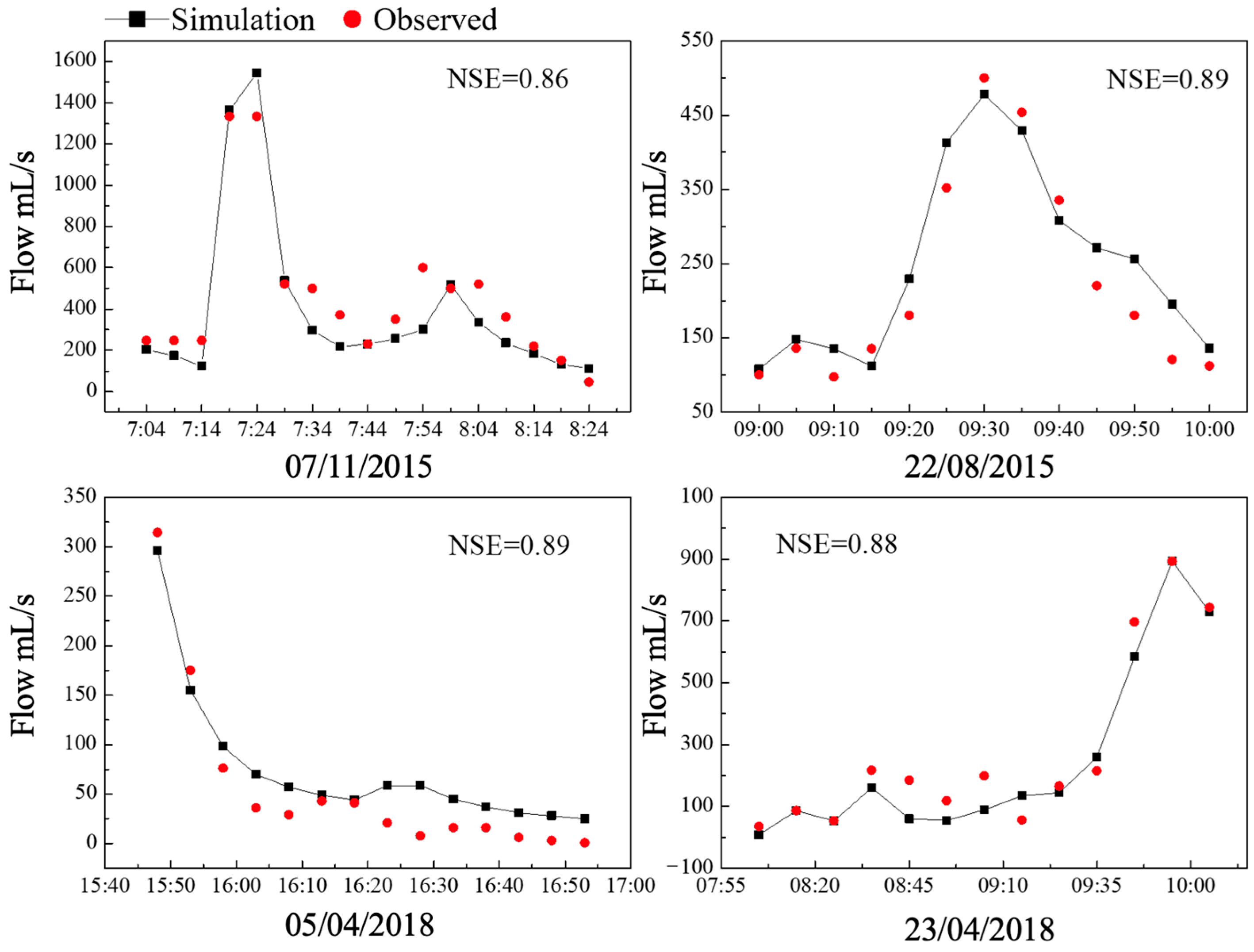
Before calibration, the sensitive parameters of the hydrologic model were selected from the InfoWorks ICM manuals, most of which suggested that the percent of impervious area and the depth of depression storage on the impervious portion of the study area were the most sensitive parameters (

Table 4. Parameters for the rainfall-runoff model.

Models	Parameters	Value
Runoff model	Runoff coefficients for impervious pavements	0.93
	F0 (Horton) initial infiltration (mm/h)	76.20
	Fc (Horton) Permeability rate (mm/h)	3.81
	K (Horton) reduction rate (L/h)	0.01
	Horton recover rate (L/h)	0.014
Routing model	Slope of the impermeable surface (m/m)	0.003
	Slope of the permeable surface (m/m)	0.00
	Manning roughness of the impermeable pavement	0.013
	Manning roughness of the permeable surface	0.15
	Initial loss the impermeable surface (mm)	0.7
	Initial loss the permeable surface (mm)	1.0

). The difference between the observed and simulated flow is shown graphically in Figure 3. The Nash–Sutcliffe model efficiency coefficients (NSEs) were 0.86, 0.89, 0.89, and 0.88 for the rainfall events on 7 November 2015, 22 August 2015, 5 April 2018, and 23 April 2018, respectively. As for the peak flow, the differences in volume and time between the observed and simulated data were less than 20%. The results indicated that the simulated runoff was in good agreement with the observed discharge and was acceptable for further analysis.

3.1.2. Water Quality Model

For the water quality model, the uncertainty analysis was conducted by the GLUE method, and the calibrated parameters are shown in Table S2.

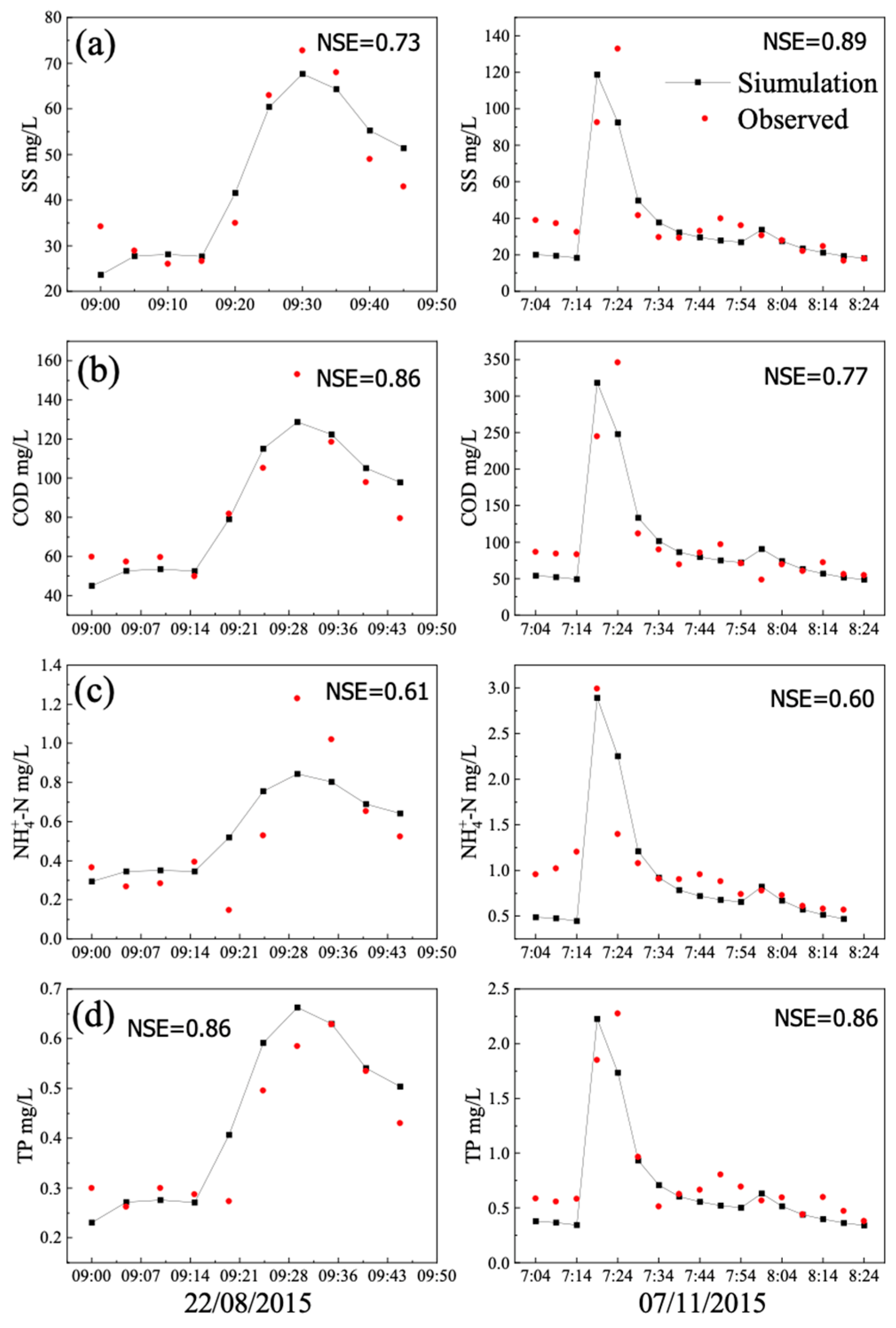
The simulations of SS, COD, and TP are acceptable; however, the modeled NH₄⁺-N concentration is not accurate enough (Figure 4). The inaccuracy in NH₄⁺-N modeling indicated that the concentration of NH₄⁺-N in runoff might not be linearly related to the concentration of SS [32]. According to the likelihood distribution of different parameters, it can be concluded that the SS simulation is most sensitive to C_3, and the NSE value plateaus when C3 falls in the range of −8 to −6. The model is not sensitive to the value of C₁, since a high NSE value always occurs whatever C1 is in the range. The COD modeling is sensitive to both ${\mathsf{\gamma }}_{1COD}$ and ${\mathsf{\gamma }}_{3COD}$, and the NSE value reaches the maximum when ${\mathsf{\gamma }}_{1COD}$ is around 1 and ${\mathsf{\gamma }}_{3COD}$ is around 0.25. For the NH₄⁺-N simulation, ${\mathsf{\gamma }}_{1{\mathrm{NH}}_4^{+}-\mathrm{N}}$ and ${\mathsf{\gamma }}_{3{\mathrm{NH}}_4^{+}-\mathrm{N}}$ are the sensitive parameters, while for TP, the sensitive parameters are ${\mathsf{\gamma }}_{1\mathrm{TP}}$ and ${\mathsf{\gamma }}_{3\mathrm{TP}}$.

Then, the upper and lower ranges of the uncertainty analysis falling within the 90% confidence interval were plotted with the observed data. The observed data for SS and COD falls in the uncertainty range, while some of the observed NH₄⁺-N and TP concentrations were not in the model’s uncertainty range. This exclusion can be explained by the assumptions of the water quality simulation in InfoWorks ICM that the concentrations of pollutants are linearly related to the concentration of SS and the coefficient is consistent in a storm event [23]. Therefore, it neglected the relationship between pollutants and rainfall characteristics and might result in errors. In addition, Deletic et al. (2012) [33] pointed out that such integrated models containing several interdependent sub-models might cause over-parametrization and enlarge the uncertainty of the models.

The model was then calibrated with rainfall events on 5 April 2018 and 23 April 2018. The NSE values of the SS and COD modeling of both rainfall events imply that the model is accurate enough; however, for NH₄⁺-N and TP modeling, with NSE values larger than 0.6 and a similar peaking time, the results can be regarded as acceptable.

3.2. Impact of LID Sizes on the Volume and Pollutant Reduction of Surface Runoff

Size is the most important parameter in LID design because it directly influences the volume and quality of the runoff in a catchment. As shown in Figure 5, when the area of the sunken green belt is enlarged, the volume reduction increases linearly; however, the pollutant reduction rate increased at first and then declined. The curve of pollutant reduction is due to the FFE, for the initial rainfall carries most of the pollutants, and the concentration of pollutants declines as the rainfall goes on. Likewise, according to the figures, the FFE increased with the increase in rainfall intensity, the runoff interception decreased, and the change in pollutant removal was negligible.

Comparing the figures in Figure 5, it can be concluded that when the peak and duration were consistent, the water quantity reduction rate decreased significantly with the increase in rainfall intensity. However, the change in water quality reduction rate was negligible. Besides, the FFE were enhanced with the increase in rainfall intensity. Therefore, even though less water was retained by the sunken green belt when the precipitation intensified, the change in intercepted pollutants was negligible.

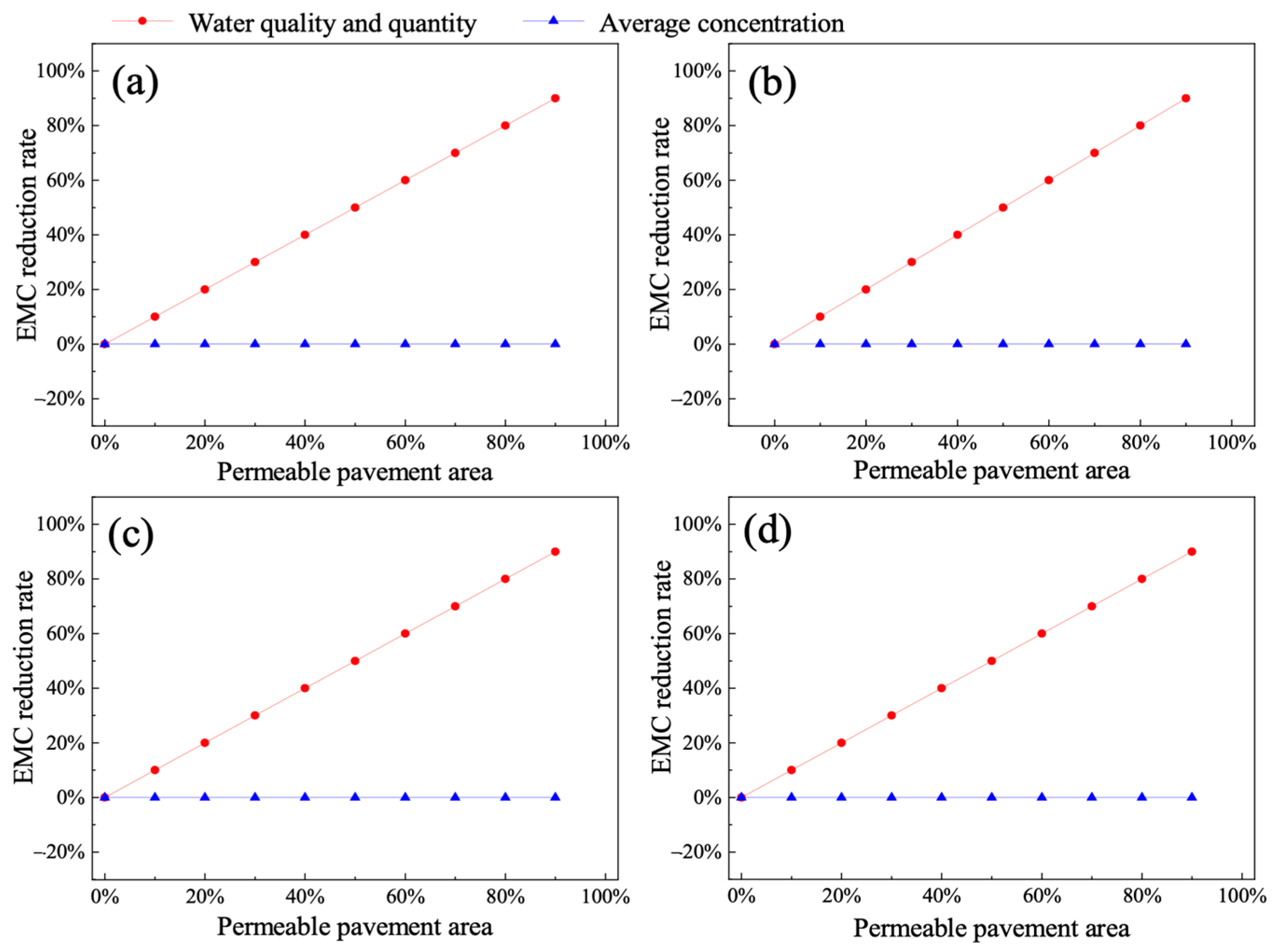
Since permeable pavements only intercept rainfall on the surface, the reduction in water quantity is directly proportional to the area of the LID facility with a slope of around one (Figure 6). The pollutants accumulated on the surface were also intercepted with the runoff, and thus the pollutant removal curve is almost the same as the quantity reduction curve.

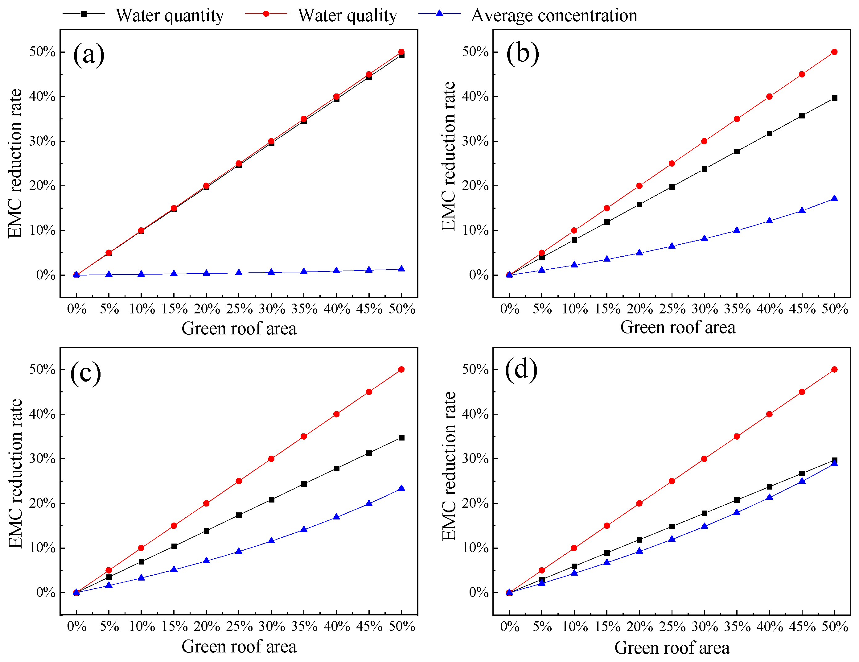
In the model, the green roof only received rainwater that fell directly on it, so the water reduction rate was proportional to the area. When the rainfall intensity increased, there would be an overflow on the green roof [34]. The water reduction rate would thereby decrease, but the changes in the pollution removal rate were negligible (Figure 7). In this model, the accumulated pollutants on the surface of green roofs were not considered. As a result, the total amount of accumulated pollutants decreases when green roofs take up more space in the study area, and therefore the pollutants in the stormwater are diminished.

3.3. Optimization of LID Facilities

For water quantity reduction, the results were fitted with a first-order polynomial equation (Equations (8) and (9)), and the value of the regression coefficients was calculated for rainfall events with a three-year and ten-year return period. The p-Value for either rainfall intensity is less than 0.0001, which indicates that the model is significant enough. For each rainfall event, since the determination coefficients R², Adj R²,and Pred R² were all 100%, the model fits perfectly.

$$f_{1three-years}\left(x\right)=1.59606+2.44357X_1+1.07443X_2+0.82593X_3$$

(8)

$$f_{1ten-years}\left(x\right)=0.93942+1.70496X_1+1.07295X_2+0.61173X_3$$

(9)

The response surfaces for runoff quantity reduction are shown in Figure S1, in which the results indicate that there were no interactions between the portion of the sunken green belt, permeable pavements, and green roof. The water reduction rate increased with any one of the above variables when other variables remained unchanged.

For pollutant removal, the regression coefficients were calculated, and the response variable was fitted with the following second-order polynomial equations:

$$\begin{array}{cc}\hfill f_{2 three-years}\left(x\right)& \\ & =-41.52042+19.28233X_1+2.23699X_2+2.23699X_3-0.15076X_1{X}_2\hfill \\ & -0.15076X_1{X}_3-0.01728X_2{X}_3-0.70556X_1^2-8.63834E^{-0.03}{X}_2^2\hfill \\ & -8.63834E^{-0.03}{X}_3^2\hfill \end{array}$$

(10)

$$\begin{array}{cc}\hfill f_{2 ten-years}\left(x\right)& \\ & =-34.15688+16.9891X_1+2.17877X_2+2.17877X_3-0.13749X_1{X}_2\hfill \\ & -0.13749X_1{X}_3-0.017156X_2{X}_3-0.5773X_1^2-8.57779E^{-0.03}{X}_2^2\hfill \\ & -8.57779E^{-0.03}{X}_3^2\hfill \end{array}$$

(11)

The ANOVA analysis indicated that the model was significant because either p-Value was smaller than 0.0001 and the Adj R² for rainfall events with different intensities was 0.9995, 0.9991, respectively. The determination coefficients (R²) for two simulated rainfall events were 99.98% and 99.96%, respectively, which indicated that the model was adequate for prediction and that only 0.02% and 0.04% of the total variation could not be explained by the model within the range of experimental variables.

The response surface analysis of runoff pollution removal rate was also considered accurate because the p values were smaller than 0.0001. The contour lines in Figure S2 were almost straight and parallel, indicating that the portion of the sunken green belt, the permeable pavement area, and the green roof had little impact on the runoff pollutant removal rate. Additionally, when other variables remained the same, the runoff pollutant removal rate increased with any one of the above variables.

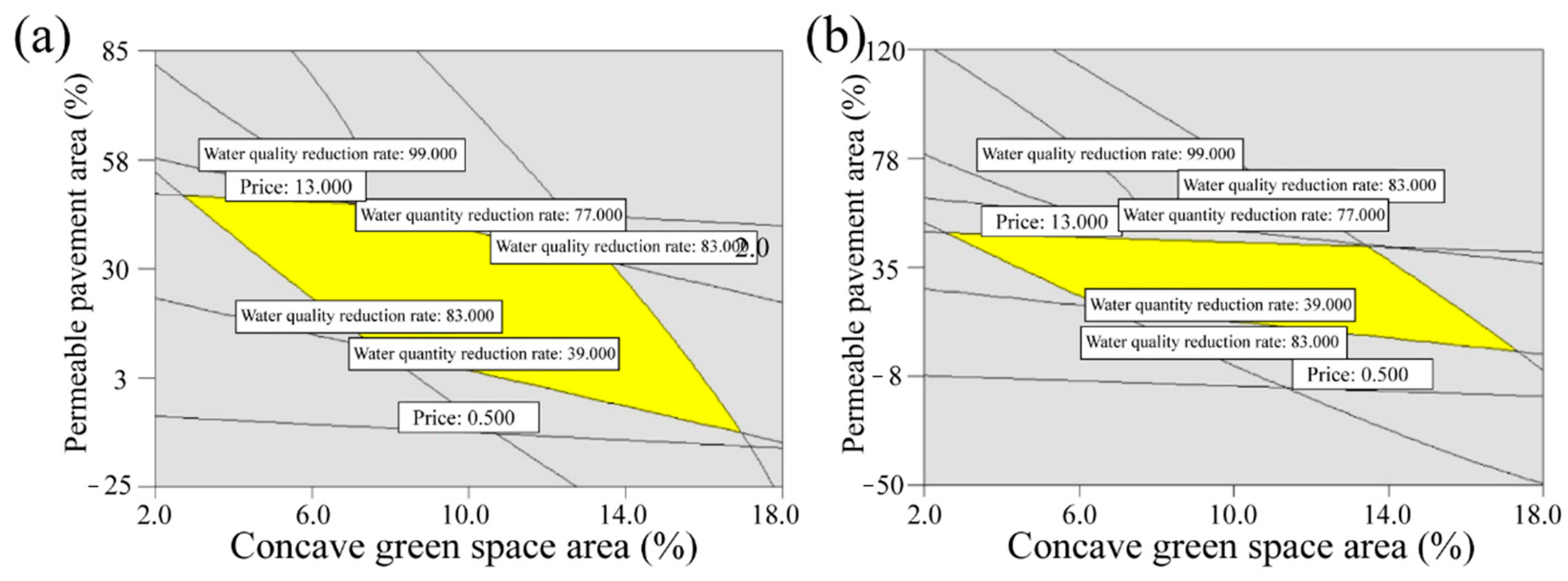
The combinatorial optimization function in Design-expert was employed to calculate the optimal LID configuration under two rainfall intensities. The optimal solutions were the overlapped areas of the contour figures (Figure 8). The maximal desirability for a 3-year return period rainfall event was 0.585. The optimal configuration of LID facilities in the investigated area was 8.6% of the sunken green belt, 15% of the permeable pavement, and 10% of the green roof, with an estimated cost of about $900,000. Under this LID design, the runoff volume reduction rate and pollutant removal rate were 47.3% and 90.4%, respectively. The outcomes were similar to the prediction values, which proved the effectiveness of the response surface method in LID design optimization.

For precipitation with a 10-year return period, the maximal expectation was 0.538. The optimal portion of the sunken green belt, permeable pavement, and green roof in the study area was 8.6%, 19%, and 10%, respectively, with a total cost of about $1,000,000. The runoff volume reduction rate and pollutant removal rate of this LID design were 42.1% and 90.9%, respectively. These results indicated that the sunken green belt was a better choice compared with permeable pavement and a green roof in terms of water quality improvement and price. Therefore, in the LID design, the sunken green belt should take priority over permeable pavement and green roof, and the optimal area of these two LID facilities needs to be calculated [35,36]. However, Shen and Xu (2021) [30] found that the runoff generated by impermeable roads drained directly into the rainwater wells and not through the green belts. Therefore, the confluence relationship between impermeable roads and green belt areas should be changed from parallel to series to improve the volume control effect on rainfall-runoff [30].

3.4. Perspectives and Limitations

This study established a rainfall-runoff model and calibrated and validated the data of real-case rainfall events in InfoWorks ICM. The impact of the sizes of these three different types of LID facilities on the water quantity as well as the water quality was examined by different rainfall events with different intensities, and the optimal design in a certain study area was determined by the response surface methodology using the Design Expert. Ho et al. (2022) [31] reported that the green roofs and permeable pavements had a higher unit cost reduction rate than the rain barrels. However, through our methods, we found that the sunken green belt was a better choice compared with permeable pavement and a green roof in terms of water quality improvement and price. Our study provided a strategy for optimizing the design of LID facilities for stormwater runoff treatment, which could provide insight into the future planning of LID facilities in urban ecosystems.

The limitations of this study lie in the water quality estimation of both the model and the LID facilities. In InfoWorks ICM, the LID facilities are only modeled to remove the pollutant from the intercepted runoff and neglect the physical removal processes, such as filtration and sedimentation. Moreover, in this research, only runoff quantity reduction, pollutant removal, and total investment were taken for optimization purposes; however, other objectives, such as social and human benefits, and difficulty in construction should be included.

4. Conclusions

This paper provided a strategy for optimizing the design of LID facilities for stormwater runoff treatment through the rainfall-runoff model and the response surface methodology. Using the GLUE method in the calibration and uncertainty analysis of the water quality model avoided equifinality and improved the accuracy of the parameters as well as the efficiency of model calibration. Results showed that LID facilities only removed pollutants in the intercepted runoff, so the initial flush effect cannot be significantly alleviated. Meanwhile, the sunken green belt was more effective and economical in reducing the runoff volume and improving runoff quality. However, for areas with limited green space, the optimal ratio of various LID facilities can be obtained from the surface response method and the overall expectation function method. The optimization process used the response surface methodology, which incorporates hydrological responses, water quality dynamics, and the investment of different LID designs. However, other objectives, such as social and human benefits and difficulty in construction, should be included in the future. This proposed methodology may be helpful in stormwater management facility planning.

References

- Saraswat, C.; Kumar, P.; Mishra, B.K. Assessment of stormwater runoff management practices and governance under climate change and urbanization: An analysis of Bangkok, Hanoi and Tokyo. Environ. Sci. Policy 2016, 64, 101–117. [Google Scholar] [CrossRef]
- Kaykhosravi, S.; Khan, U.T.; Jadidi, A. A Comprehensive Review of Low Impact Development Models for Research, Conceptual, Preliminary and Detailed Design Applications. Water 2018, 10, 1541. [Google Scholar] [CrossRef] [Green Version]
- Krisnayanti, D.S.; Rozari, P.d.; Garu, V.C.; Damayanti, A.C.; Legono, D.; Nurdin, H. Analysis of Flood Discharge due to Impact of Tropical Cyclone. Civ. Eng. J. 2022, 8, 1752–1763. [Google Scholar] [CrossRef]
- Shi, H.; Yin, D.; Li, X.; Gong, Y.; Li, J. Urban stormwater runoff thermal characteristics and mitigation effect of low impact development measures. J. Water Clim. Chang. 2019, 10, 53–62. [Google Scholar] [CrossRef]
- Chen, Z.; Shi, X.; Zhang, J.; Wu, L.; Wei, W.; Ni, B.-J. Nanoplastics are significantly different from microplastics in urban waters. Water Res. X 2023, 19, 100169. [Google Scholar] [CrossRef] [PubMed]
- Hong, J.; Lee, B.; Park, C.; Kim, Y. A colorimetric detection of polystyrene nanoplastics with gold nanoparticles in the aqueous phase. Sci. Total Environ. 2022, 850, 158058. [Google Scholar] [CrossRef] [PubMed]
- Luo, T.; Dai, X.; Chen, Z.; Wu, L.; Wei, W.; Xu, Q.; Ni, B.-J. Different microplastics distinctively enriched the antibiotic resistance genes in anaerobic sludge digestion through shifting specific hosts and promoting horizontal gene flow. Water Res. 2023, 228, 119356. [Google Scholar] [CrossRef]
- Chen, Z.; Wei, W.; Liu, X.; Ni, B.J. Emerging electrochemical techniques for identifying and removing micro/nanoplastics in urban waters. Water Res. 2022, 221, 118846. [Google Scholar] [CrossRef] [PubMed]
- Chow, M.F.; Yusop, Z. Sizing first flush pollutant loading of stormwater runoff in tropical urban catchments. Environ. Earth Sci. 2014, 72, 4047–4058. [Google Scholar] [CrossRef]
- Wang, M.; Zhang, D.; Adhityan, A.; Ng, W.J.; Dong, J.; Tan, S.K. Assessing cost-effectiveness of bioretention on stormwater in response to climate change and urbanization for future scenarios. J. Hydrol. 2016, 543, 423–432. [Google Scholar] [CrossRef]
- Suwarno, I.; Ma’arif, A.; Raharja, N.M.; Nurjanah, A.; Ikhsan, J.; Mutiarin, D. IoT-based lava flood early warning system with rainfall intensity monitoring and disaster communication technology. Emerg. Sci. J. 2021, 4, 154–166. [Google Scholar] [CrossRef]
- Baek, S.S.; Choi, D.H.; Jung, J.W.; Lee, H.J.; Lee, H.; Yoon, K.S.; Cho, K.H. Optimizing low impact development (LID) for stormwater runoff treatment in urban area, Korea: Experimental and modeling approach. Water Res. 2015, 86, 122–131. [Google Scholar] [CrossRef]
- Abduljaleel, Y.; Demissie, Y. Identifying Cost-Effective Low-Impact Development (LID) under Climate Change: A Multi-Objective Optimization Approach. Water 2022, 14, 3017. [Google Scholar] [CrossRef]
- Rong, Q.; Liu, Q.; Xu, C.; Yue, W.; Su, M. Optimal configuration of low impact development practices for the management of urban runoff pollution under uncertainty. J. Environ. Manag. 2022, 320, 115821. [Google Scholar] [CrossRef] [PubMed]
- Jeon, M.; Guerra, H.B.; Choi, H.; Kim, L.-H. Long-Term Monitoring of an Urban Stormwater Infiltration Trench in South Korea with Assessment Using the Analytic Hierarchy Process. Water 2022, 14, 3529. [Google Scholar] [CrossRef]
- Kaykhosravi, S.; Khan, U.T.; Jadidi, M.A. The Effect of Climate Change and Urbanization on the Demand for Low Impact Development for Three Canadian Cities. Water 2020, 12, 1280. [Google Scholar] [CrossRef]
- Chuang, W.-K.; Lin, Z.-E.; Lin, T.-C.; Lo, S.-L.; Chang, C.-L.; Chiueh, P.-T. Spatial allocation of LID practices with a water footprint approach. Sci. Total Environ. 2023, 859, 160201. [Google Scholar] [CrossRef]
- Lee, J.M.; Park, M.; Min, J.-H.; Kim, J.; Lee, J.; Jang, H.; Na, E.H. Evaluation of SWMM-LID Modeling Applicability Considering Regional Characteristics for Optimal Management of Non-Point Pollutant Sources. Sustainability 2022, 14, 14662. [Google Scholar] [CrossRef]
- Xiong, L.; Xu, Z.; Xu, J. Combined Optimization of LID Patches and the Gray Drainage System to Control Wet Weather Discharge Pollution. ACS ES&T Water 2022, 2, 1734–1746. [Google Scholar] [CrossRef]
- Gironás, J.; Roesner, L.A.; Rossman, L.A.; Davis, J. A new applications manual for the Storm Water Management Model (SWMM). Environ. Modell. Softw. 2010, 25, 813–814. [Google Scholar] [CrossRef]
- Li, J.; Zhang, B.; Mu, C.; Chen, L. Simulation of the hydrological and environmental effects of a sponge city based on MIKE FLOOD. Environ. Earth Sci. 2018, 77, 32. [Google Scholar] [CrossRef]
- Rosa, D.J.; Clausen, J.C.; Dietz, M.E. Calibration and Verification of SWMM for Low Impact Development. JAWRA J. Am. Water Resour. Assoc. 2015, 51, 746–757. [Google Scholar] [CrossRef]
- He, Q.; Chai, H.; Yan, W.; Shao, Z.; Zhang, X.; Deng, S. An integrated urban stormwater model system supporting the whole life cycle of sponge city construction programs in China. J. Water Clim. Chang. 2019, 10, 298–312. [Google Scholar] [CrossRef]
- Li, J.; Deng, C.; Li, Y.; Li, Y.; Song, J. Comprehensive Benefit Evaluation System for Low-Impact Development of Urban Stormwater Management Measures. Water Resour. Manag. 2017, 31, 4745–4758. [Google Scholar] [CrossRef]
- Fan, G.; Lin, R.; Wei, Z.; Xiao, Y.; Shangguan, H.; Song, Y. Effects of low impact development on the stormwater runoff and pollution control. Sci. Total Environ. 2022, 805, 150404. [Google Scholar] [CrossRef] [PubMed]
- Zhang, Z.; Gu, J.; Zhang, G.; Ma, W.; Zhao, L.; Ning, P.; Shen, J. Design of urban runoff pollution control based on the Sponge City concept in a large-scale high-plateau mountainous watershed: A case study in Yunnan, China. J. Water Clim. Chang. 2021, 12, 201–222. [Google Scholar] [CrossRef] [Green Version]
- Kong, F.; Ban, Y.; Yin, H.; James, P.; Dronova, I. Modeling stormwater management at the city district level in response to changes in land use and low impact development. Environ. Modell. Softw. 2017, 95, 132–142. [Google Scholar] [CrossRef]
- Urich, C.; Rauch, W. Modelling the urban water cycle as an integrated part of the city: A review. Water Sci. Technol. 2014, 70, 1857–1872. [Google Scholar] [CrossRef] [PubMed]
- Li, M.; Yang, X. Global Sensitivity Analysis of SWMM Parameters Based on Sobol Method. China Water Wastewater 2020, 36, 95–102. [Google Scholar]
- Shen, H.B.; Xu, Z.X. Monitoring and Evaluating Rainfall-Runoff Control Effects of a Low Impact Development System in Future Science Park of Beijing. J. Am. Water Resour. Assoc. 2021, 57, 638–651. [Google Scholar] [CrossRef]
- Ho, H.C.; Lee, H.Y.; Tsai, Y.J.; Chang, Y.S. Numerical Experiments on Low Impact Development for Urban Resilience Index. Sustainability 2022, 14, 8696. [Google Scholar] [CrossRef]
- de Macedo, M.B.; Pereira de Oliveira, T.R.; Oliveira, T.H.; Gomes Junior, M.N.; Texeira Brasil, J.A.; Ferreira do Lago, C.A.; Mendiondo, E.M. Evaluating low impact development practices potentials for increasing flood resilience and stormwater reuse through lab-controlled bioretention systems. Water Sci. Technol. 2021, 84, 1103–1124. [Google Scholar] [CrossRef] [PubMed]
- Deletic, A.; Dotto, C.B.S.; McCarthy, D.T.; Kleidorfer, M.; Freni, G.; Mannina, G.; Uhl, M.; Henrichs, M.; Fletcher, T.D.; Rauch, W.; et al. Assessing uncertainties in urban drainage models. Phys. Chem. Earth Parts A/B/C 2012, 42-44, 3–10. [Google Scholar] [CrossRef] [Green Version]
- Ouellet, V.; Khamis, K.; Croghan, D.; Gonzalez, L.M.H.; Rivera, V.A.; Phillips, C.B.; Packman, A.I.; Miller, W.M.; Hawke, R.G.; Hannah, D.M.; et al. Green roof vegetation management alters potential for water quality and temperature mitigation. Ecohydrology 2021, 14, e2321. [Google Scholar] [CrossRef]
- Malekinezhad, H.; Sepehri, M.; Hosseini, S.Z.; Santos, C.A.G.; Rodrigo-Comino, J.; Meshram, S.G. Role and Concept of Rooftop Disconnection in Terms of Runoff Volume and Flood Peak Quantity. Int. J. Environ. Res. 2021, 15, 935–946. [Google Scholar] [CrossRef]
- Koc, K.; Ekmekcioglu, O.; Ozger, M. An integrated framework for the comprehensive evaluation of low impact development strategies. J. Environ. Manag. 2021, 294, 113023. [Google Scholar] [CrossRef]
Figure 1.
Map of the study area: (a) location of Jiangsu Province in China; (b) location of Yixing City in Jiangsu Province; (c) the DEM (Digital Elevation Model) of Yixing City; (d) study area; (e) simulated image of InfoWorks ICM.
Figure 2.
Flowchart for optimizing LID size.
Figure 3.
Observed and simulated flow rates in calibration.
Figure 4.
Observed and simulated (a) SS, (b) COD, (c) NH4+-N, (d) TP concentrations in calibration.
Figure 5.
The impact of the sunken green belt on runoff water quality and quantity. (a) rainfall intensity once a year. (b) rainfall intensity once every three years. (c) rainfall intensity once every five years. (d) rainfall intensity once every ten years.
Figure 6.
The impact of permeable pavement area on runoff water quality and quantity. (a) rainfall intensity once a year. (b) rainfall intensity once every three years. (c) rainfall intensity once every five years. (d) rainfall intensity once every ten years.
Figure 7.
The impact of green roof area on runoff water quality and quantity. (a) rainfall intensity once a year. (b) rainfall intensity once every three years. (c) rainfall intensity once every five years. (d) rainfall intensity once every ten years.
Figure 8.
Contour overlay diagram. (a) rainfall intensity once every three years. (b) rainfall intensity once every ten years.