3.2. Changes in Hydrometeorological Parameters
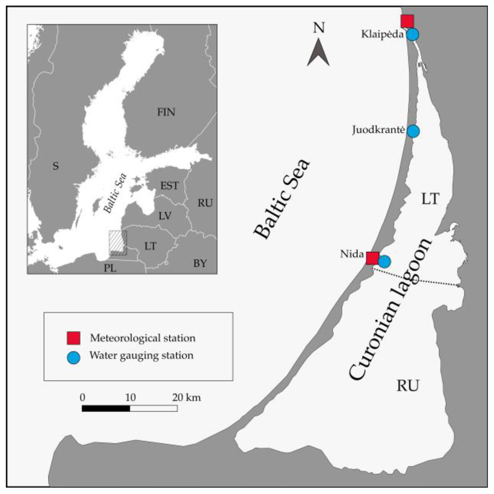
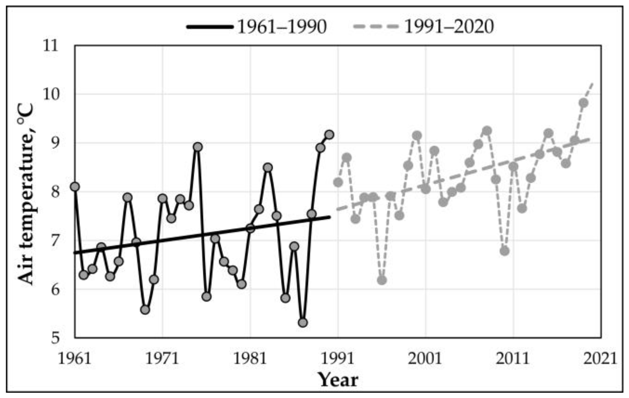
Air temperature. Air temperature analysis at the Curonian Lagoon was carried out based on Klaipėda and Nida meteorological station data. As can be seen from
Figure 2, in the first period, the average annual air temperature was 7.1 °C (ranging from 5.3 to 9.2 °C in individual years), and in the second period, 8.4 °C (ranging from 6.2 to 10.2 °C). It increased by 0.029 °C yr
−1 in 1961–1990 (statistically insignificant increase,
p > 0.05) and by 0.046 °C yr
−1 in 1991–2020 (statistically significant increase,
p = 0.007). Over the entire study period, the air warmed by an average of 0.041 °C yr
−1 (
p = 0.0001).
The trends of air temperature over the selected periods were analyzed by the Mann–Kendall test. Average air temperatures, Sen’s slopes and
p values are provided in
Table 2; they represent different seasons (winter consists of December, January and February; spring of March, April and May; summer of June, July and August; autumn of September, October and November). Air temperature during the studied period increased the most in winter and spring (Sen’s slope 0.063 and 0.053, respectively). The slight upward direction of its values was estimated in autumn (Sen’s slope 0.007) and a slight downward trend in the summer months (Sen’s slope −0.017). However, the estimated rise was statistically insignificant, as the Mann–Kendall test indicated
p values greater than 0.05 for all periods. The situation was somewhat different in the following period: the air temperature went up the most in autumn (Sen’s slope 0.079), a little bit less in the summer and spring months (Sen’s slope 0.047 and 0.041, respectively) and the least in the winter season (Sen’s slope 0.007). The positive trend in the second 30-year period was significant only in summer and autumn, as
p values reached 0.032 and 0.001, respectively;
p values were higher than 0.05 in the remaining seasons. A comparison of the air temperature between the two periods revealed that it increased the most in winter (1.7 °C), slightly less in spring and summer (1.4 °C, respectively), and the least in autumn (0.5 °C).
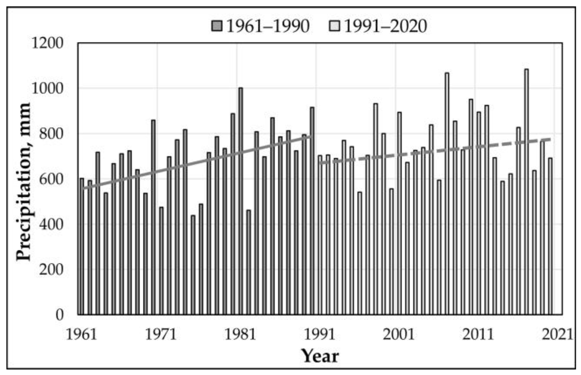
Precipitation. The average precipitation was calculated using Klaipėda and Nida MS data. From the data in
Figure 3, it is apparent that the change in precipitation was uneven. During the first period, it ranged from 438 (in 1975) to 1001 mm (in 1981), and in the second, from 541 (in 1996) to 1083 mm (in 2017). Its annual average was 709 and 764 mm, respectively. According to statistical analysis, precipitation increased by 6.6 mm yr
−1 in 1961–1990 and by 3.1 mm yr
−1 in 1991–2020 (
Table 3). However, this tendency was statistically reliable only in 1961–1990 (
p = 0.011), whereas in 1991–2020, the increase was statistically insignificant (
p > 0.05).
As for the seasonal values, the analysis revealed that in the first 30-year period, precipitation had positive trends in all seasons. It increased the most in autumn (Sen’s slope 4.11) and significantly less during the winter and summer seasons (Sen’s slope 2.31 and 1.38, respectively), while the slightest shift to higher values was estimated in spring (Sen’s slope 0.31) (
Table 3). Over the recent 30-year period, precipitation trends were the most pronounced in summer (Sen’s slope 2.01). The average change (but of a different pattern: Sen’s slope was 1.34 and −1.29, respectively) was determined in the winter and spring seasons. Precipitation changed the least in autumn (Sen’s slope 0.10). When comparing the two periods, statistically significant differences were identified only in the winter and autumn of the first period (
p value 0.012 and 0.037, respectively). Precipitation increased the most in winter (43.9 mm) and in the remaining seasons—slightly (up to 5.3 mm) (
Table 3).
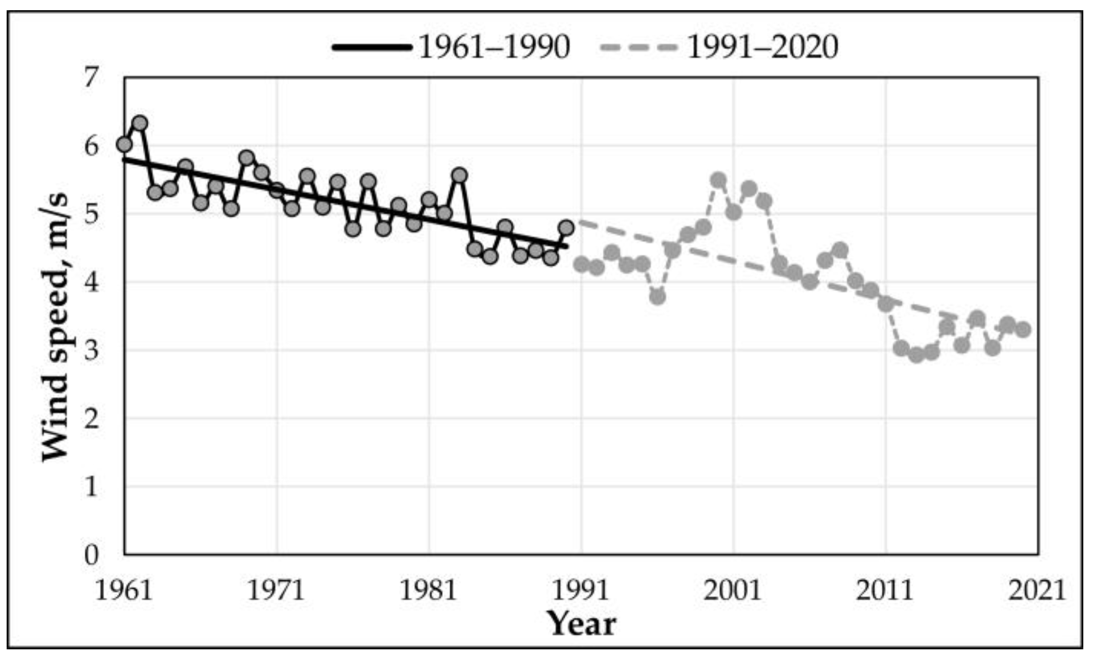
Wind parameters. The analysis of wind parameters (speed and direction) at the Curonian lagoon was based on the data recorded in Klaipėda MS. As
Figure 4 shows, the wind speed decreased: its average value in the first period was 5.1 m/s and ranged from 4.3 m/s in 1989 to 6.3 m/s in 1962; in the second period, it varied from 2.9 m/s in 2013 to 5.5 m/s in 2000, averaging 4.1 m/s. Wind speed declined by 0.041 m/s yr
−1 in 1961–1990 and by 0.055 m/s yr
−1 in 1991–2020.
The analysis of seasonal trends in wind speed indicated that this variable experienced the most pronounced changes among all studied meteorological parameters of the lagoon (
Table 4). In the first 30-year period, wind speed declined almost equally in the spring, summer and autumn seasons; Sen’s slope values were −0.051, −0.054 and −0.047, respectively, whereas in winter, the changes were significantly lower (Sen’s slope was only −0.025). The Mann–Kendall test revealed that in all seasons, except for winter, these changes were statistically significant;
p values varied from 0.0001 to 0.004. In the second period, on the contrary, the most considerable changes were determined in the winter season (Sen’s slope 0.076). In the spring, summer, and autumn seasons, the wind speed decreased very similarly as in the first period, and the Sen’s slope values were −0.047, −0.042 and −0.055, respectively. The downward trend in wind speed values in the recent period was statistically significant, and the
p values of different seasons varied from 0.0001 to 0.002. Overall, it was found that wind speed diminished the most in autumn, by 1.6 m/s. Meanwhile, it decreased quite similarly in the remaining seasons, by 1.1, 0.9 and 0.8 m/s, respectively.
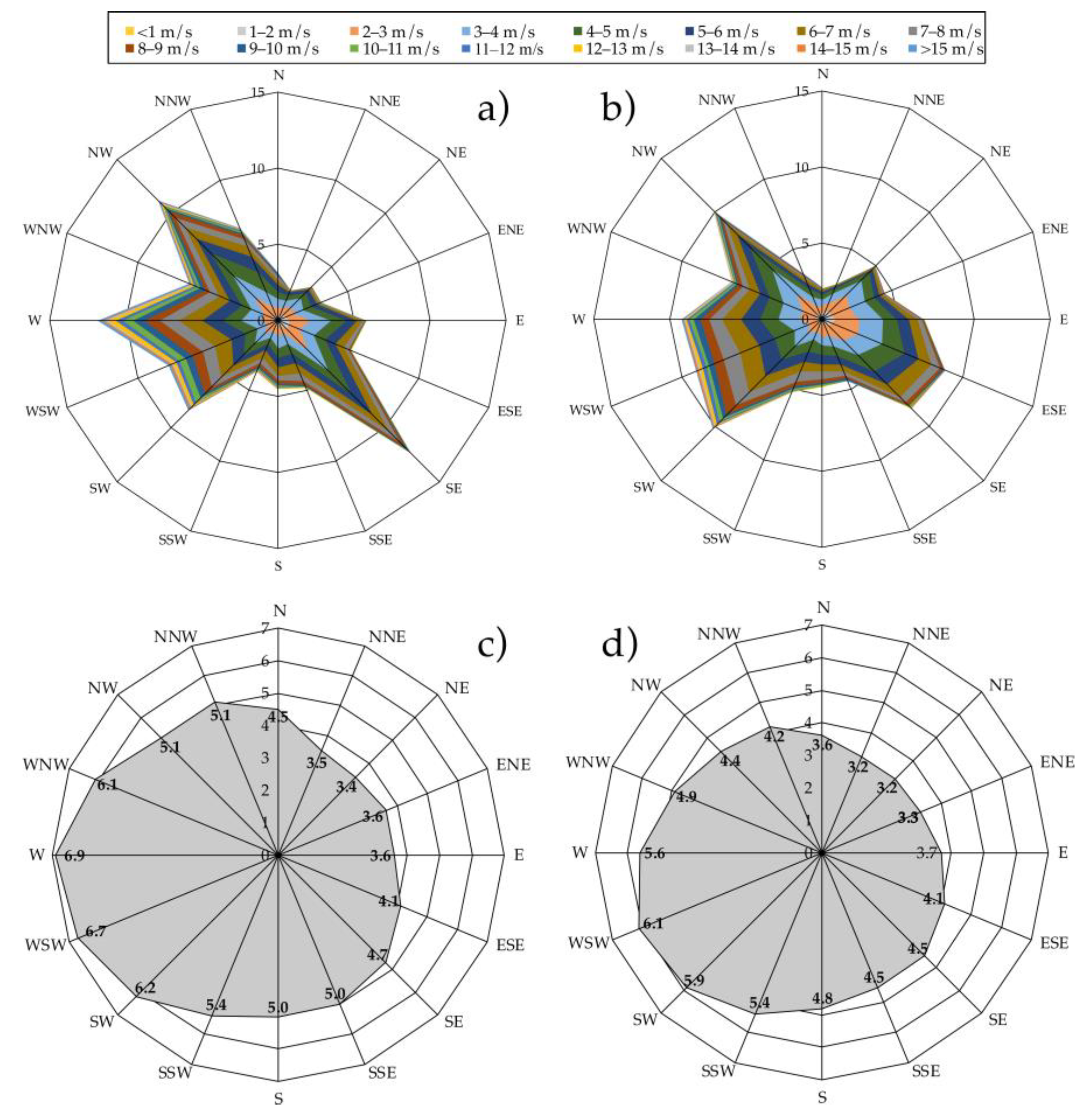
Another critical indicator is the recurrence of certain wind directions and the average wind speed of a certain direction. As shown in
Figure 5, in the first thirty years, the observed winds were mainly from SE, W, NW and SW. However, the strongest winds blew from W, WSW, SW and WNW. Their average speeds were 6.9, 6.7, 6.2 and 6.1 m/s, respectively (
Figure 5c). During the second thirty-year period, the prevailing wind directions changed slightly, resulting in the increased frequency of NW, SW, W and WSW winds (
Figure 5b). During this period, the strongest winds were from WSW, SW, W and SSW. Their speed reached 6.1, 5.9, 5.6 and 5.4 m/s, respectively (
Figure 5c).
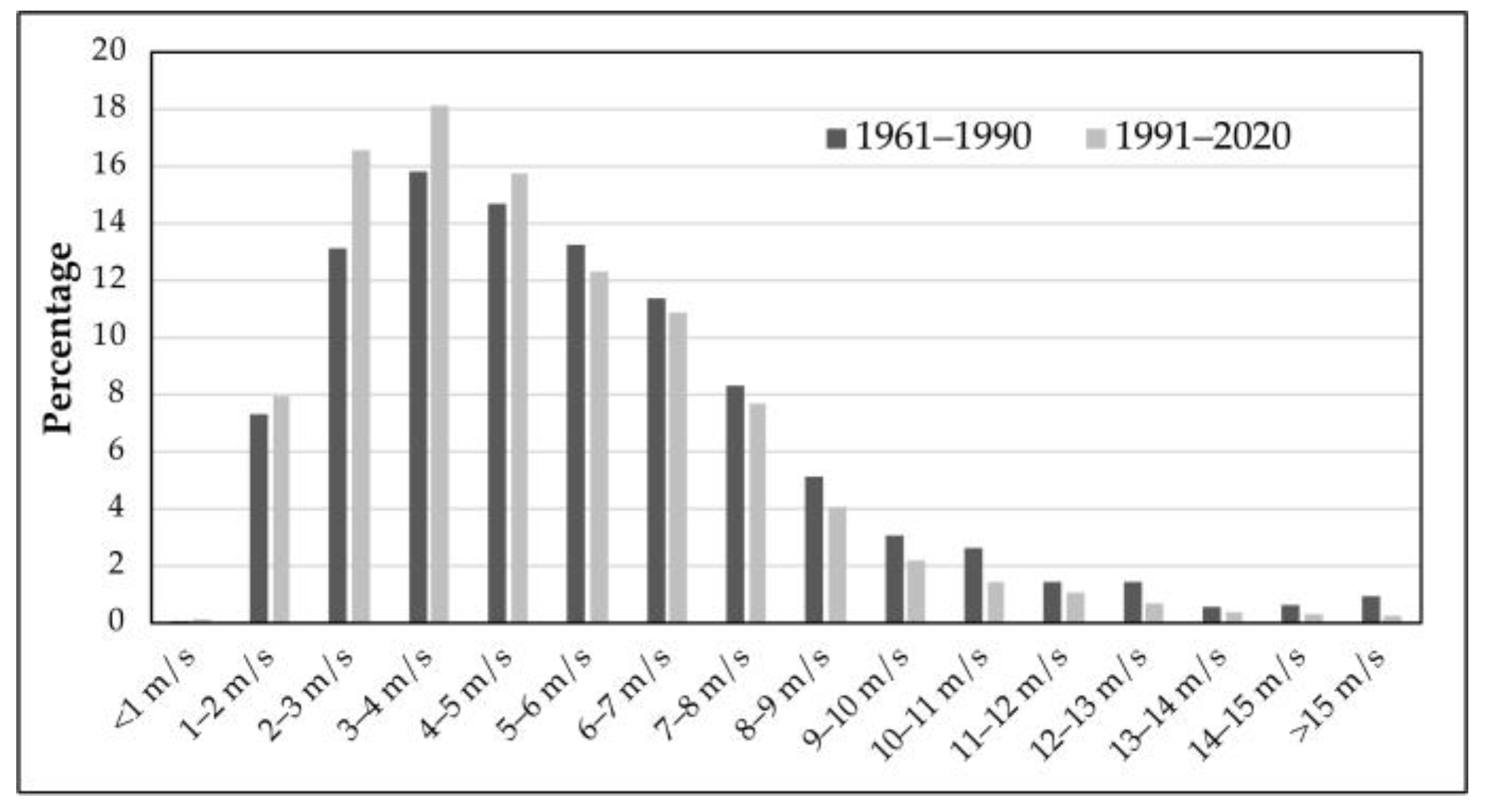
When analyzing wind indicators, it is important to know the average wind speed and direction and how often winds of particular strength were observed. Wind speeds of 2 to 6 m/s prevailed throughout the entire observation period (
Figure 6). These winds accounted for 56.9% of all investigated cases in the first period and 62.8% in the second. The frequency of winds weaker than 2 m/s and stronger than 6 m/s in the first and second periods was very similar, 37.2% and 43.1%, respectively. Winds up to 5 m/s increased recently, but the winds stronger than 5 m/s decreased. This decrease is particularly pronounced in the range of winds stronger than 10 m/s (
Figure 6).
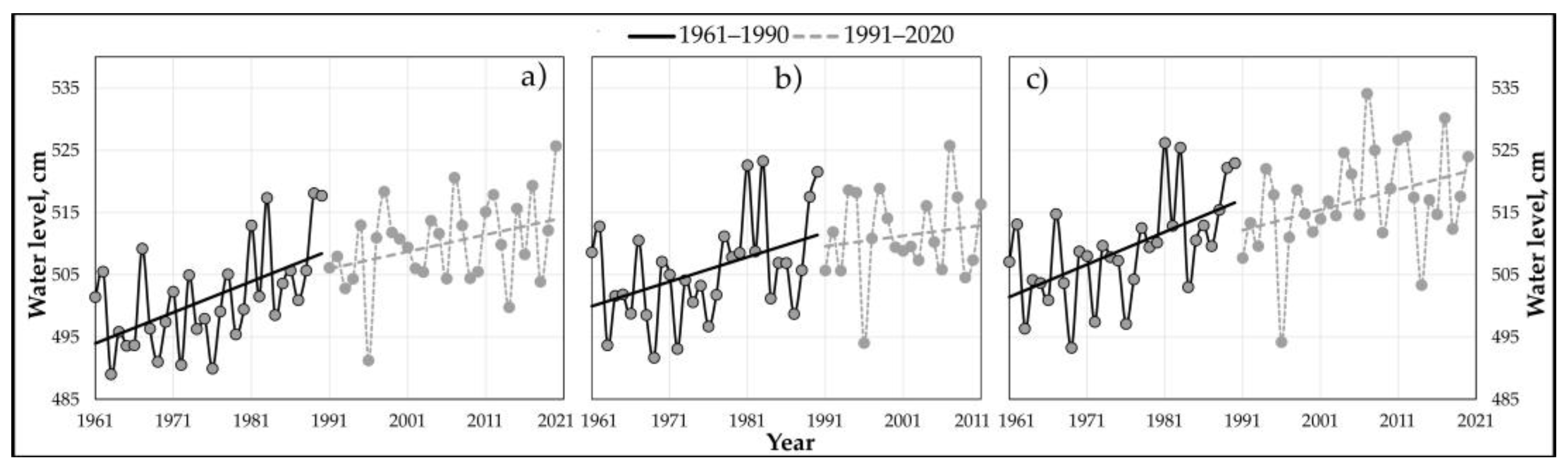
Water level. The analysis of the water level of the Curonian Lagoon was carried out according to the data of Klaipėda, Juodkrantė and Nida WGSs. Water level data from Juodkrantė were used only until the end of 2011, as this station was closed later. The analysis revealed that the highest water level is characteristic of the southern part of the lagoon (at Nida), while it gradually decreases toward the Klaipėda Strait (
Figure 7). In 1961–1990, the average lagoon level at Nida was 509 cm and varied from 493 to 526 cm (
Figure 7c). During the same period, the average water level at Juodkrantė was 506 cm. In individual years, it varied between 492 and 523 cm (
Figure 7b). The lowest average annual water level was at Klaipėda at 501 cm and varied from 489 to 518 cm (
Figure 7a). In the first period, water level rose in all studied stations. On average, water level increased annually by 0.32 cm at Juodkrantė, 0.47 cm at Klaipėda and 0.48 cm at Nida.
In the recent period of 1991–2020, the average water level at Nida was 517 cm, and in individual years, its annual values varied from 494 to 534 cm (
Figure 7c). According to the available data (until 2011), it was 511 cm at Juodkrantė and varied from 494 to 526 cm (
Figure 7b). The average annual water level at Klaipėda in 1961–1990 was 510 cm and fluctuated between 491 and 526 cm (
Figure 7a). In the last 30 years, the water level in all studied stations increased, but not as fast as in 1961–1990. At Juodkrantė, it went up by 0.11 cm yr
−1, at Klaipėda by 0.19 cm yr
−1 and at Nida by 0.28 cm yr
−1.
The average water level for different time spans at Klaipėda, Juodkrantė and Nida, Sen’s slopes and
p values are presented in
Table 5. In the first period, the variation of the water level in different stations could be characterized by the same patterns. This parameter increased the most in winter, less in autumn and summer and the least in the spring season. At Juodkrantė, water level data exhibited statistically insignificant positive trends (
p > 0.05). At Klaipėda and Nida, they were insignificant only in spring (
p > 0.05), while in other seasons, the
p value varied from 0.013 to 0.032 (
Table 5). However, when analyzing the water level values in the second period, no common regularities between individual WGSs were found. According to Klaipėda WGS data, the lagoon level rose the most in winter, less in autumn and spring, and least in summer. At Juodkrantė, it increased in summer and autumn but decreased in other seasons. At Nida, same as at Klaipėda, positive changes were estimated in the second 30-year period. The water level increased the most in summer and autumn and least in other seasons. Considering the results of the Mann–Kendall test, the detected changes were statistically insignificant as
p > 0.05. Throughout the entire period, according to the records of all WGSs, the lagoon water level rose. The most remarkable shift to higher values was observed in spring and winter, 9.9 and 9.6 cm, respectively, and slightly less at 8.1 cm in summer.
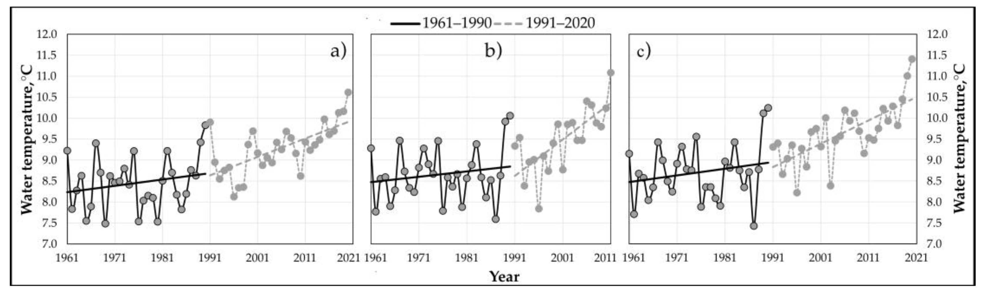
Water temperature. The analysis of the lagoon water temperature was carried out using data from Klaipėda, Juodkrantė (until 2011) and Nida WGSs. The average annual water temperature is presented in
Figure 8. In 1961–1990, its lowest value was observed at Klaipėda, where the lagoon connects to the Baltic Sea. Here, it reached 8.4 °C and varied from 7.5 (1969) to 9.8 °C (1990). Moving away from Klaipėda Strait, the water temperature increased. At Juodkrantė, during the studied period, it averaged 8.6 °C and varied from 7.6 (1987) to 10.1 °C (1990). At Nida, it was the highest, 8.7 °C, and ranged from 7.7 (1962) to 10.2 °C (1990) (
Figure 8c). In the second period (1991–2020), the lowest average water temperature was also at Klaipėda, 9.2 °C, and it increased moving away from the strait. It was 9.4 °C at Juodkrantė and 9.7 °C at Nida. At Klaipėda, this parameter varied from 8.1 (1996) to 10.2 °C (2019), at Juodkrantė from 7.8 (1996) to 11.1 °C (2011), and at Nida from 8.2 (1996) to 11.4 °C (2020) (
Figure 8). Therefore, during the entire period, the average annual water temperature of the Curonian Lagoon showed rising trends. In the first 30-year period, the increase was not statistically significant. However, in the second period, water temperature increased from 0.047 to 0.070 °C per year, and these changes were statistically significant (
p value < 0.000).
In the first period, the lagoon surface temperature had mixed trends in different seasons (
Table 6). At all investigated stations, the temperature decreased in autumn (Sen’s slope varied from −0.001 to −0.011), and at Klaipėda and Juodkrantė, also in summer (Sen’s slope ranged from −0.0004 to −0.021). However, rising water temperature trends prevailed for the rest of the seasons (Sen’s slope varied from 0.007 to 0.036). Only at Klaipėda was the increase statistically significant (
p = 0.011) in winter; in all other cases,
p was greater than 0.05. In the second period, water temperature changes had a positive sign, but no common trends were identified. Minor changes were detected at Klaipėda in winter (Sen’s slope 0.006) and the largest at Juodkrantė in autumn (Sen’s slope 0.118). The identified changes were statistically insignificant at all stations in winter (in the case of Juodkrantė also in spring,
p > 0.05) but significant in the remaining seasons (
p < 0.05). The findings showed that the water surface temperature of the lagoon rose least in winter and autumn (respectively, 0.5 and 0.6 °C) and the most in summer and spring (respectively, 1.1 and 1.0 °C).
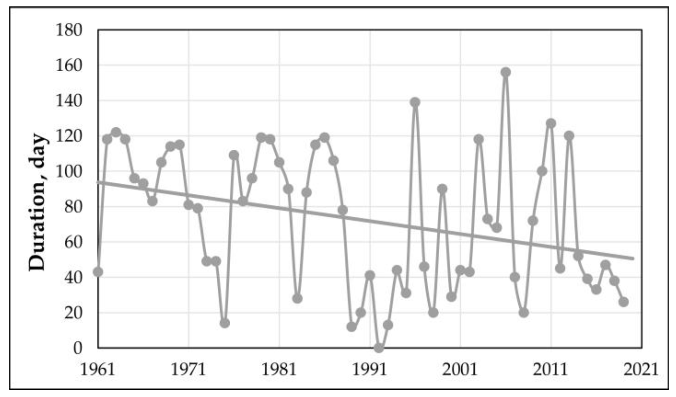
Ice parameters. Data from Nida (1961–2020) were used to analyze the changes in the ice cover on the lagoon. In the port of Klaipėda, a constant ice cover does not form due to shipping; therefore, data from this station were not taken into account. From 1961 to 1990, the permanent ice cover was observed for an average of 86 days, while in 1991–2020, it lasted only 59 days (
Figure 9). The duration of ice cover varied greatly in individual years, from 12 to 122 days in the first period and from 0 to 156 days in the second (
Figure 9). Based on the data from long-term observations, it was established that the duration of the ice cover on the Curonian Lagoon decreased by 2.5 days every three years (0.82 days annually). The shortening of ice cover duration was statistically significant only during the entire analyzed period of 1961–2020 (
p value 0.02), while in 1961–1990 and 1991–2020,
p was greater than 0.05.
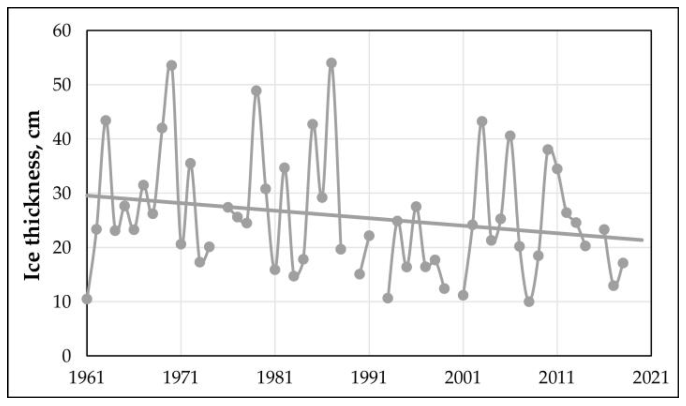
As we can see from
Figure 10, some years have missing data on ice thickness. In these cases, the lagoon was covered with such a thin layer of ice that measurements could not be taken for safety reasons. During the first period, the average thickness of the lagoon ice cover was 28.5 cm and varied from 10.5 (1961) to 54.0 cm (1987) (
Figure 10). During the following period, it was 22.4 cm and ranged between 10.0 cm in 2008 and 43.3 cm in 2003 (
Figure 10). Ice cover thinned by 0.14 cm annually during the whole analyzed period. Even though the lagoon ice thickness was decreasing, statistical analysis revealed that these changes in the selected periods (1961–2020, 1961–1990, and 1991–2020) were statistically insignificant,
p > 0.05.
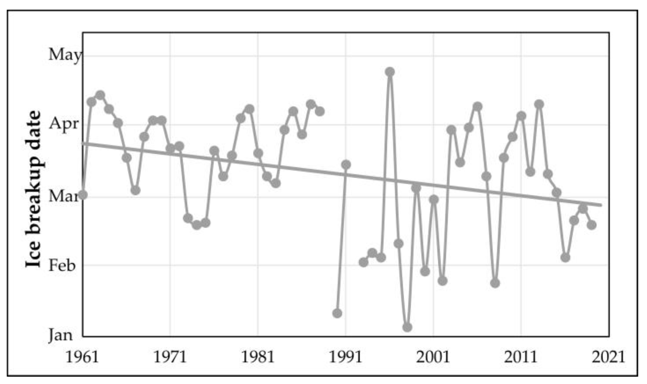
The breakup time of the ice also changed over time.
Figure 11 shows that in the first 30 years, the ice melted on average on March 19 and during the second 30-year period on March 1. However, the freeze-up dates varied considerably from year to year. In the first period, the ice melted on 17 February at the earliest and on 13 April at the latest. Meanwhile, during the second period, the years with the earliest (4 January) and the latest ice breakup (22 April) were identified. Despite the large scatter in the recent period (1991–2020), the ice breakup dates showed a negative trend, and the ice melt date moved forward by four days every nine years (or 0.44 days per year). The advance of breakup dates was statistically significant only in 1961–2020 (at
p value 0.03). Changes in both periods were statistically insignificant,
p > 0.05.


